Tied links and invariants for singular links

Abstract.

Tied links and the tied braid monoid were introduced recently by the authors and used to define new invariants for classical links. Here, we give a version purely algebraic–combinatoric of tied links. With this new version we prove that the tied braid monoid has a decomposition like a semi–direct group product. By using this decomposition we reprove the Alexander and Markov theorem for tied links; also, we introduce the tied singular knots, the tied singular braid monoid and certain families of Homflypt type invariants for tied singular links; these invariants are five–variables polynomials. Finally, we study the behavior of these invariants; in particular, we show that our invariants distinguish non isotopic singular links indistinguishable by the Paris–Rabenda invariant.

1. Introduction

Tied links and their algebraic counterpart, the tied braid monoid, were introduced by the authors in [2]. A tied link is a classical link admitting ties among its components; the tied braid monoid is defined through a presentation with usual braid generators together with ties generators and defining relations coming from the so–called bt–algebra [1], cf. [2, 19, 17, 12].

Tied links contains the classical links, so every invariant for tied links defines also an invariant for classical links. We have constructed two invariants for tied links: the one of type Homflypt polynomial [2] and the other one of type Kauffman polynomial [4]. These invariants turn out to be more powerful, respectively, than the Homflypt and the Kauffman polynomials; therefore the tied links are useful in the understanding of classical links. These invariants for tied links were constructed by the Jones recipe and also by skein relations. In the construction using the Jones recipe, the role played by the tied braid monoid is to tied links as the role of the braid groups to the classical links.

With the aim of constructing others classes of tied knot–like objects, we reformulate the tied links in algebraic–combinatoric terms, and we prove that the tied braid monoid has a certain decomposition as semi–direct product: a part formed by ties (monoid of the set partitions) and the other part by the usual braid (braid group). This decomposition and the new algebraic–combinatoric context for tied links allows us to introduce the tied singular links and combinatoric tied singular links. Hence we define four families of invariants for combinatoric tied singular links which are constructed by the Jones recipe by using two maps from the singular braid monoid to the bt–algebra and two different presentations of this algebra. These invariants are five–variables polynomials of type Homflypt, in the sense that they become the Hompflypt polynomial whenever are evaluated on classical knots. We define these invariants also by skein relations; the usual ‘local skein relations’, which take into account any two crossing strands, are replaced by ‘global skein relations’, which take into account also the components to which the crossing strands belong.

We also study here the behavior of these invariants, that is, we compare them with each other and with another invariant for singular links of type Homflypt polynomial, defined by Paris and Rabenda in [18] which is a four–variable polynomial that generalizes the invariant defined by Kauffman y Vogel in [15]. As we said before, the importance of tied links lies in the fact that, when evaluated on classical links, they are able to distinguish pairs of isotopic links not distinguished by classical polynomials, see [3], [4], [5] and [9]. Now, we have to notice that, as far as we know, in literature there is not a list of non isotopic singular links which are not distinguished by the known invariants for singular links. Therefore, we build pairs of singular links starting by some pairs of non isotopic classical links that are not distinguished by the Homflypt polynomial, according to the list provided in [8], then we calculate on them our invariants and the invariant due to Paris and Rabenda [15]. We remark, finally, that in general it seems to be not easy to find pairs proving that the new polynomials are more powerful on singular links.

We give now the layout of the paper. Section 2 establishes the main tools used during the paper, that is, some facts on set partitions and the bt–algebra. The main goal of Section 3, is to prove Theorem 2, which says that the tied braid monoid $TB_{n}$ can be decomposed as the semi–direct product, denoted by $\mathsf{P}_{n}\rtimes B_{n}$, between the monoid $\mathsf{P}_{n}$, formed by the set partition of $\{1,\ldots,n\}$ and the braid group $B_{n}$; note that the action of $B_{n}$ on $\mathsf{P}_{n}$ is naturally inherited from the action of the symmetric group on $\mathsf{P}_{n}$. The decomposition of $TB_{n}$ as semi–direct product uses several ideas of [19] adapted to our situation. Now, the decomposition of $TB_{n}$ by the monoid $\mathsf{P}_{n}$, a monoid eminently combinatoric, and the group $B_{n}$, induces to treat the tied links as algebraic–combinatoric objects, the combinatoric tied links, which are introduced in Section 4; we define also their isotopy classes, which of course coincide with those of tied links. In Theorems 4 and 5 we prove, respectively, the Markov and Alexander theorems for combinatoric tied links.

In Section 5 we recall some elements from the the theory of singular links; also we introduce four families of invariants for singular links, see Theorems 7 and 8. These are five–variables polynomials, which we denote by $\Phi_{\mathsf{x},\mathsf{y}\,}$, $\Psi_{\mathsf{x},\mathsf{y}\,}$, $\Phi_{\mathsf{x},\mathsf{y}\,}^{\prime}$ and $\Psi_{\mathsf{x},\mathsf{y}\,}^{\prime}$; notice that the letters $\mathsf{x}$ and $\mathsf{y}\,$ are two of the five variables of the invariants but they parametrize the invariants too. These invariants come out from the Jones recipe; more precisely, we construct homomorhpisms from the monoid of singular braids to the bt–algebra (Proposition 6), so using these homomorphisms and the Markov trace on the bt–algebra [3], we derive the invariants after the usual method of rescaling and normalization originally due to V. Jones [13].

Section 6 introduces the tied singular link which is nothing more than a classical singular link with ties, or, equivalently, a tied link with some singular crossings. We define then the combinatoric tied singular links, for short cts–links. This definition (Definition 13) is the natural extension of the combinatoric tied links (Definition 5). The algebraic counterpart of cts–links is provided: the monoid of tied singular links (Definition 14). This monoid, denoted by $TSB_{n}$, is defined trough a presentation; however, we prove in Theorem 9 that it can be obtained, in the same way as $TB_{n}$, as a semidirect product, denoted by $\mathsf{P}_{n}\rtimes SB_{n}$, between $\mathsf{P}_{n}$ and the singular braid monoid $SB_{n}$ [6, 7, 20]. The section ends proving, respectively, in Theorems 10 and 11 the Alexander and Markov theorem for cts–links.

Section 7 has two subsections: in the first one, we lifts the invariants $\Phi_{\mathsf{x},\mathsf{y}\,}$, $\Psi_{\mathsf{x},\mathsf{y}\,}$, $\Phi_{\mathsf{x},\mathsf{y}\,}^{\prime}$ and $\Psi_{\mathsf{x},\mathsf{y}\,}^{\prime}$ to cts–links, this is done simply by extending the domain of the defining morphism of these invariants from $SB_{n}$ to $TSB_{n}$. This is a simple matter since $TSB_{n}$ is decomposed as $\mathsf{P}_{n}\rtimes SB_{n}$, see Proposition 8. In the second subsection, we prove respectively in Theorems 12, 13 and 14, that the invariants $\Phi_{\mathsf{x},\mathsf{y}\,}$, $\Psi_{\mathsf{x},\mathsf{y}\,}$, $\Phi^{\prime}_{\mathsf{x},\mathsf{y}\,}$ and $\Psi^{\prime}_{\mathsf{x},\mathsf{y}\,}$ can be defined through skein rules.

Section 8 is devoted to the comparisons of the invariants defined here among them and and also with the four–variable polynomial invariant for singular links defined by Paris and Rabenda in [18]. Notably, Theorem 15 clarifies the differences between the $\Phi_{\mathsf{x},\mathsf{y}\,}$’s the $\Psi_{\mathsf{x},\mathsf{y}\,}$’s with respect to the parameters $\mathsf{x}$ and $\mathsf{y}\,$. Finally, in Theorems 16, 17 and Propositions 11 and 12, we give examples showing that our invariants are more powerful than the Paris–Rabenda invariant.

2. Preliminaries

In the present section we recall principally the definitions and main facts on set partitions and on the bt–algebra. The paper is in fact based on these objects.

2.1. Set partitions

For $n\in{\mathbb{N}}$, we denote by ${\bf n}$ the set $\{1,\ldots,n\}$ and by $\mathsf{P}_{n}$ the set formed by the set partitions of ${\bf n}$, that is, an element of $\mathsf{P}_{n}$ is a collection $I=\{I_{1},\ldots,I_{k}\}$ of pairwise–disjoint non–empty sets whose union is ${\bf n}$; the sets $I_{1},\ldots,I_{k}$ are called the blocks of $I$; the cardinal of $\mathsf{P}_{n}$, denoted $b_{n}$, is called the $n^{th}$ Bell number. Further, $(\mathsf{P}_{n},\preceq)$ is a poset with partial order defined as follows: $I\preceq J$ if and only if each block of $J$ is a union of blocks of $I$.

We shall use the following scheme of a set partition in $\mathsf{P}_{n}$, according to the standard representation by arcs, see [16, Subsection 3.2.4.3], that is: the point $i$ is connected by an arc to the point $j$, if $j$ is the minimum in the same block of $i$ satisfying $j>i$. In Figure 1 a set partition in representation by arcs.

Figure 1. Scheme of the partition $I=\{\{1,3\},\{2,5,6\},\{4\}\}$.

The representation by arcs of a set partition induces a natural indexation of its blocks. More precisely, we say that the blocks $I_{j}$’s of the set partition $I=\{I_{1},\ldots,I_{m}\}$ of ${\bf n}$ are standard indexed if $\min(I_{j})<\min(I_{j+1})$, for all $j$. For instance, in the set partition of Figure 1 the blocks are indexed as: $I_{1}=\{1,3\}$, $I_{2}=\{2,5,6\}$ and $I_{3}=\{4\}$.

As usual we denote by $S_{n}$ the symmetric group on $n$ symbols and we set $s_{i}=(i,i+1)$. The permutation action of $S_{n}$ on ${\bf n}$ inherits, in the obvious way, an action of $S_{n}$ on $\mathsf{P}_{n}$ that is, for $I=\{I_{1},\ldots,I_{m}\}$ we have

$$w(I):=\{w(I_{1}),\ldots,w(I_{m})\}.$$ (1)

Notice that this action preserves the cardinal of each block of the set partition.

We shall say that two set partitions $I$ and $I^{\prime}$ in $\mathsf{P}_{n}$ are conjugate, denoted by $I\sim I^{\prime}$, if there exits $w\in S_{n}$ such that, $I^{\prime}=w(I)$; if it is necessary to precise such $w$, we write $I\sim_{w}I^{\prime}$. Further, observe that if $I$ and $I^{\prime}$ are standard indexed with $m$ blocks, then the permutation $w$ induces a permutation $w_{I,I^{\prime}}$ of $S_{m}$ acting on the indices of the blocks.

Example 1.

Let $I=\{\{1,2\}_{1},\{3\}_{2},\{4,5\}_{3},\{6\}_{4}\}$ and $I^{\prime}=\{\{1\}_{1},\{2,5\}_{2},\{3,6\}_{3}\{4\}_{4}\}$, so $n=6$ and $m=4$. We have $I\sim_{w}I^{\prime}$, where:

$$w=(1,6)(2,3,4,5)\quad\text{and}\quad w_{I,I^{\prime}}=(1,3,2,4).$$

Given a permutation $w\in S_{n}$ and writing $w=c_{1}\cdots c_{m}$ as product of disjoint cycles, we denote by $K_{w}$ the set partition whose blocks are the cycles $c_{i}$’s, regarded now as subsets of $\bf n$. Reciprocally, given a set partition $I=\{I_{1},\ldots,I_{m}\}$ of $\bf n$ we denote by $w_{I}$ an element of $S_{n}$ whose cycles are the blocks $I_{i}$’s. Moreover, we shall say that the cycles of $w_{I}$ are standard indexed, if they are indexed according to the standard indexation of $I$.

Notation 1.

When there is no risk of confusion, we will omit in the partitions the blocks with a single element.

2.2. The bt–algebra

Let $\mathsf{u}\,$ be an indeterminate and set ${\mathbb{K}}={\mathbb{C}}(\mathsf{u}\,)$.

Definition 1 (See [1, 19, 3]).

The bt–algebra , denoted by $\mathcal{E}_{n}(\mathsf{u}\,)$, is defined by $\mathcal{E}_{1}(\mathsf{u}\,):={\mathbb{K}}$ and for $n\geq 2$ as the unital associative ${\mathbb{K}}$–algebra, with unity $1$, defined by braid generators $T_{1},\ldots,T_{n-1}$ and ties generators $E_{1},\ldots,E_{n-1}$ subjected to the following relations:

$$E_{i}E_{j} = E_{j}E_{i}\qquad\text{ for all $i,j$},$$ (2)

$$E_{i}^{2} = E_{i}\qquad\text{ for all $i$},$$ (3)

$$E_{i}T_{j} = T_{j}E_{i}\qquad\text{for $|i-j|>1$},$$ (4)

$$E_{i}T_{i} = T_{i}E_{i}\qquad\text{ for $|i-j|=1$},$$ (5)

$$E_{i}T_{j}T_{i} = T_{j}T_{i}E_{i}\qquad\text{ for $|i-j|=1$},$$ (6)

$$E_{i}E_{j}T_{i} = E_{j}T_{i}E_{j}\quad=\quad T_{i}E_{i}E_{j}\qquad\text{ for $|i-j|=1$},$$ (7)

$$T_{i}T_{j} = T_{j}T_{i}\qquad\text{ for $|i-j|>1$},$$ (8)

$$T_{i}T_{j}T_{i} = T_{j}T_{i}T_{j}\qquad\text{ for $|i-j|=1$},$$ (9)

$$T_{i}^{2} = 1+(u-1)E_{i}+(u-1)E_{i}T_{i}\qquad\text{ for all $i$}.$$ (10)

Notice that every $T_{i}$ is invertible, and

$$T_{i}^{-1}=T_{i}+(u^{-1}-1)E_{i}+(u^{-1}-1)E_{i}T_{i}.$$ (11)

The bt–algebra is finite dimensional. Moreover, there is a basis defined by S. Ryom–Hansen; we describe here the construction of this basis, because some elements of it admit analogous that will be used in Section 2.

For $i<j$, we define $E_{i,j}$ by

$$E_{i,j}=\left\{\begin{array}[]{ll}E_{i}&\text{for}\quad j=i+1\\ T_{i}\cdots T_{j-2}E_{j-1}T_{j-2}^{-1}\cdots T_{i}^{-1}&\text{otherwise.}\end{array}\right.$$ (12)

For any nonempty subset $J$ of $\bf n$ we define $E_{J}=1$ for $|J|=1$ and otherwise by

$$E_{J}:=\prod_{(i,j)\in J\times J,i<j}E_{i,j}.$$

Note that $E_{\{i,j\}}=E_{i,j}$. For $I=\{I_{1},\ldots,I_{m}\}\in\mathsf{P}_{n}$, we define $E_{I}$ by

$$E_{I}=\prod_{k}E_{I_{k}}.$$ (13)

Now, if $w=s_{i_{1}}\cdots s_{i_{k}}$ is a reduced expression of $w\in S_{n}$, then the element $T_{w}:=T_{i_{1}}\cdots T_{i_{k}}$ is well defined. The action of $S_{n}$ on $\mathsf{P}_{n}$ is inherited from the $E_{I}$’s and we have:

$$T_{w}E_{I}T_{w}^{-1}=E_{w(I)}\qquad(\text{see \cite[cite]{[\@@bibref{}{rhJAC}{}{}, Corollary 1]}}).$$ (14)

Theorem 1.

[19, Corollary 3] The set $\{E_{I}T_{w}\,;\,w\in S_{n},\,I\in\mathsf{P}_{n}\}$ is a ${\mathbb{K}}$–linear basis of ${\mathcal{E}}_{n}(\mathsf{u}\,)$. Hence the dimension of ${\mathcal{E}}_{n}(\mathsf{u}\,)$ is $b_{n}n!$.

The theorem above implies that ${\mathcal{E}}_{n}(\mathsf{u}\,)\subseteq{\mathcal{E}}_{n+1}(\mathsf{u}\,)$, for all $n$. Denote ${\mathcal{E}}_{\infty}(\mathsf{u}\,)$ the inductive limit associated to these inclusions and by $\rho$ the Markov trace defined on ${\mathcal{E}}_{\infty}(\mathsf{u}\,)$. More precisely, fixing two commutative independent variables $\mathsf{a}\,$ and $\mathsf{b}\,$, we have the following theorem.

Theorem 2.

[3, Theorem 3] There exists a unique family $\rho:=\{\rho_{n}\}_{n\in{\mathbb{N}}}$, where $\rho_{n}$’s are linear maps, defined inductively, from $\mathcal{E}_{n}(\mathsf{u}\,)$ in $\mathbb{K}[\mathsf{a}\,,\mathsf{b}\,]$ such that $\rho_{n}(1)=1$ and satisfying, for all $X,Y\in\mathcal{E}_{n}(\mathsf{u}\,)$, the following rules:

1. $\rho_{n}(XY)=\rho_{n}(YX)$,

2. $\rho_{n+1}(XT_{n})=\rho_{n+1}(XT_{n}E_{n})=\mathsf{a}\,\rho_{n}(X)$,

3. $\rho_{n+1}(XE_{n})=\mathsf{b}\,\rho_{n}(X)$.

Remark 1.

Extending the field ${\mathbb{K}}$ to ${\mathbb{K}}(\mathsf{v}\,)$ with $\mathsf{v}\,^{2}=\mathsf{u}\,$, we can define (cf. [17, Subsection 2.3]):

$$V_{i}:=T_{i}+(\mathsf{v}\,^{-1}-1)E_{i}T_{i}.$$ (15)

Then the $V_{i}$’s and the $E_{i}$’s satisfy the relations (4)–(9) and the quadratic relation (10) is transformed in

$$V_{i}^{2}=1+(\mathsf{v}\,-\mathsf{v}\,^{-1})E_{i}V_{i}.$$ (16)

So,

$$V_{i}^{-1}=V_{i}-(\mathsf{v}\,-\mathsf{v}\,^{-1})E_{i}.$$ (17)

In [9, 10, 12] this quadratic relation is used to define the bt–algebra. Although at algebraic level these algebras are the same, we will see that they lead on to different invariants. Thus, in order to distinguish these two presentations of the bt–algebra, we will write $\mathcal{E}_{n}(\mathsf{v}\,)$ when the bt–algebra is defined by using the quadratic relation (16).

3. The tied braids monoid

The goal of this section is to prove Theorem 3 which says that the tied braid monoid $TB_{n}$ [2], defined originally by generators and relations, can be realized as a monoid constructed from the monoid of set partitons of ${\bf n}$ and the braid group on $n$–strand.

3.1. The monoid of set partitions

The set $\mathsf{P}_{n}$ has a structure of commutative monoid with product $\ast$. More precisely, the product $I\ast J$ between $I$ and $J$ is defined as the minimal set partition, containing $I$ and $J$, according to $\preceq$; the identity of this monoid is ${\mathbb{1}}_{n}:=\{\{1\},\{2\},\ldots,\{n\}\}$. Observe that:

$$I\ast J=J,\quad\text{whenever}\quad I\preceq J,$$ (18)

$$I\ast J=I\ast w_{I}(J).$$ (19)

For every $1\leq i<j\leq n$ with $i\not=j$, define $\mu_{i,j}\in\mathsf{P}_{n}$ as the set partition whose blocks are $\{i,j\}$ and $\{k\}$ where $1\leq k\leq n$ and $k\not=i,j$. We shall write $\mu_{i,j}\mu_{k,h}$ instead of $\mu_{i,j}\ast\mu_{k,h}$; we have

$$\mu_{i,j}^{2}=\mu_{i,j}\quad\text{and }\quad\mu_{i,j}\mu_{r,s}=\mu_{r,s}\mu_{i,j}.$$ (20)

Moreover, we have the following proposition.

Proposition 1.

The monoid $\mathsf{P}_{n}$ is generated by set partitions $\mu_{i,j}$’s.

Definition 2.

We denote by $\mathsf{P}_{\infty}$, the inductive limit monoid associated to the family $\{(\mathsf{P}_{n},\iota_{n})\}_{n\in\mathbb{N}}$, where $\iota_{n}$ is the monoid monomorphisms from $\mathsf{P}_{n}$ into $\mathsf{P}_{n+1}$, such that for $I\in\mathsf{P}_{n}$, the image $\iota_{n}(I)\in\mathsf{P}_{n+1}$ is defined by adding to $I$ the block $\{n+1\}$. Observe that the inclusions preserve $\preceq$, that is, if $I\preceq J$ for $I,J\in\mathsf{P}_{n}$, then $I\preceq J$ when $I,J$ are considered as elements of $\mathsf{P}_{n+1}$.

3.2. The tied braid monoid

Denote $B_{n}$ the braid group on $n$–strand, that is the group presented by the elementary braids $\sigma_{1},\ldots,\sigma_{n-1}$ subjected to the following relations: $\sigma_{i}\sigma_{j}=\sigma_{j}\sigma_{i}$ for all $i,j$ s.t. $|i-j|>1$ and $\sigma_{i}\sigma_{i+1}\sigma_{i}=\sigma_{i+1}\sigma_{i}\sigma_{i+1}$ for $1\leq i\leq n-2$.

Recall now that we have a natural epimorphism $\pi:B_{n}\longrightarrow S_{n}$ defined by mapping $\sigma_{i}$ to $s_{i}$. We denote by $\pi_{\alpha}$ the image of $\alpha$ by $\pi$; thus $\pi_{\sigma_{i}}=\pi_{\sigma_{i}^{-1}}=s_{i}$. The epimorphism $\pi$ defines an action of $B_{n}$ on $\mathsf{P}_{n}$: namely, the result of $\beta\in B_{n}$, acting on $I\in\mathsf{P}_{n}$, is $\pi_{\beta}(I)$, see (1). This action of $B_{n}$ on $\mathsf{P}_{n}$ defines a monoid structure on the cartesian product $\mathsf{P}_{n}\times B_{n}$, where the multiplication is defined as follows,

$$(I,\alpha)(J,\beta)=(I\ast\pi_{\alpha}(J),\alpha\beta).$$ (21)

We shall denote this monoid by $\mathsf{P}_{n}\rtimes B_{n}$. Note that $B_{n}$ and $\mathsf{P}_{n}$ can be regarded as submonoids of $\mathsf{P}_{n}\rtimes B_{n}$. More precisely, an element $\beta\in B_{n}$ correspond to $(1,\beta)$ (which will be denoted simply by $\beta$ if there is no risk of confusion); an element $I\in\mathsf{P}_{n}$ corresponds to the element $\widetilde{I}:=(I,1)$. The decomposition $(I,\beta)=(I,1)(1,\beta)$, together with the Proposition 1, implies that $\mathsf{P}_{n}\rtimes B_{n}$ is generated by the $\widetilde{\mu}_{i,j}$’s and the $\sigma_{i}$’s. Now, we also have, by eq. (21):

$$(1,\beta)(I,1)(1,\beta^{-1})=(\pi_{\beta}(I),1).$$ (22)

Thus, by taking $I=\mu_{i,i+1}$ and $\beta=\sigma_{j-1}\sigma_{j-1}\cdots\sigma_{i+1}$ with $j>i+1$, we deduce that every generator $\widetilde{\mu}_{i,j}$ can be written as a word in the $\widetilde{\mu}_{i,i+1}$ and $\sigma_{i+1}^{\pm 1},\ldots,\sigma_{j-1}^{\pm 1}$, since, for $j>i+1$

$$\mu_{i,j}=s_{j-1}s_{j-2}\cdots s_{i+1}(\mu_{i,i+1}).$$

Hence we have the following lemma.

Lemma 1.

The monoid $\mathsf{P}_{n}\rtimes B_{n}$ is generated by $\widetilde{\mu}_{1,2},\ldots,\widetilde{\mu}_{n-1,n},\sigma_{1}^{\pm 1},\ldots,\sigma_{n-1}^{\pm 1}$.

We will see below that $\mathsf{P}_{n}\rtimes B_{n}$ is the tied braid monoid $T\!B_{n}$ introduced in [2].

Definition 3.

[2, Definition 3.1] $T\!B_{n}$ is the monoid generated by the elementary braids $\sigma_{1}^{\pm 1},\ldots,\sigma_{n-1}^{\pm 1}$ and the generators $\eta_{1},\ldots,\eta_{n-1}$, called ties, such the $\sigma_{i}$’s satisfy braid relations among them together with the following relations:

$$\eta_{i}\eta_{j} = \eta_{j}\eta_{i}\qquad\text{ for all $i,j$},$$ (23)

$$\eta_{i}\sigma_{i} = \sigma_{i}\eta_{i}\qquad\text{ for all $i$},$$ (24)

$$\eta_{i}\sigma_{j} = \sigma_{j}\eta_{i}\qquad\text{for $|i-j|>1$},$$ (25)

$$\eta_{i}\sigma_{j}\sigma_{i} = \sigma_{j}\sigma_{i}\eta_{j}\qquad\text{ for $|i-j|=1$},$$ (26)

$$\eta_{i}\sigma_{j}\sigma_{i}^{-1} = \sigma_{j}\sigma_{i}^{-1}\eta_{j}\qquad\text{ for $|i-j|=1$},$$ (27)

$$\eta_{i}\eta_{j}\sigma_{i} = \eta_{j}\sigma_{i}\eta_{j}\quad=\quad\sigma_{i}\eta_{i}\eta_{j}\qquad\text{ for $|i-j|=1$},$$ (28)

$$\eta_{i}\eta_{i} = \eta_{i}\qquad\text{ for all $i$}.$$ (29)

Following the construction of Ryom–Hansen’s basis we obtain that the elements of $T\!B_{n}$ can be written in the form $\eta_{I}\beta$, where $\beta\in B_{n}$ and $\eta_{I}$’s are defined analogously to the $E_{I}$’s. We are going now to explain this fact.

As in (12), for $1\leq i<j\leq n$, we put $\eta_{i,j}:=\eta_{i}$ for $j=i+1$, and otherwise

$$\eta_{i,j}:=\sigma_{i}\sigma_{i+1}\cdots\sigma_{j-2}\eta_{j-1}\sigma_{j-2}^{-1}\cdots\sigma_{i-1}^{-1}\sigma_{i}^{-1}.$$

For every $i,j$ define $\eta_{\{i,j\}}=\eta_{\min\{i,j\},\max\{i,j\}}$. We get the following lemma.

Lemma 2.

For all $i<j$ and $k$ we have:

1. $\sigma_{k}\eta_{i,j}\sigma_{k}^{-1}=\eta_{\{s_{k}(i),s_{k}(j)\}}$,

2. $\sigma_{k}^{-1}\eta_{i,j}\sigma_{k}=\eta_{\{s_{k}(i),s_{k}(j)\}}$,

3. $\eta_{i,j}=\sigma_{j-1}^{-1}\cdots\sigma_{i+1}^{-1}\eta_{i}\sigma_{i+1}\cdots\sigma_{j-1}$,

4. $\alpha\eta_{i,j}=\eta_{\{s(i),s(k)\}}\alpha$, for $\alpha\in B_{n}$ and $s:=\pi_{\alpha}$,

5. The elements $\eta_{i,j}$’s are commuting and idempotent,

6. $\eta_{i,j}\eta_{j,k}=\eta_{i,j}\eta_{i,k}=\eta_{i,k}\eta_{j,k}=\eta_{i,j}\eta_{j,k}\eta_{i,k}$ for all $i<j<k$.

Proof.

The proof of claims (1) and (2) are the same as the proof of [19, Lemma 2] but using now relation (27) instead [19, Lemma 1].

Claims (3) and (4) are direct consequences of (1) and (2).

The proof of (5) is analogous to the proof of [19, Lemma 3].

The proof of (6) is contained in the proof of [19, Lemma 5]. ∎

For every (non–empty) subset $M$ of $\bf n$, we define $\eta_{M}$= 1 if $|M|=1$, otherwise

$$\eta_{M}:=\prod_{(i,j)\in M^{2}:i<j}\eta_{i,j}.$$ (30)

Now, for $I=\{I_{1},\ldots,I_{m}\}\in\mathsf{P}_{n}$, define $\eta_{I}$ as follows

$$\eta_{I}:=\prod_{j}\eta_{I_{j}}.$$ (31)

Let $X\subseteq{\bf n}\times{\bf n}$. Observe that $X$ defines an equivalence relation on ${\bf n}$ by setting: $i\sim_{X}i$ and $i\sim_{X}j$ if and only if there is a chain $i=i_{1},i_{2},\dots,i_{m}=j$ with $m>1$ in $X$ such that either $(i_{r},i_{r+1})\in X$ or $(i_{r+1},i_{r})\in X$. Denote $\langle X\rangle$ the partition of ${\bf n}$ determined by $\sim_{X}$.

Lemma 3.

For $X\subseteq{\bf n}\times{\bf n}$, we have

$$\eta_{\langle X\rangle}=\prod_{(i,j)\in X}\eta_{\{i,j\}}.$$ (32)

Proof.

It follows from claim (6) of Lemma 2, see [19, Lemma 5]. ∎

Proposition 2.

The elements of $T\!B_{n}$ can be written in the form $\eta_{I}\beta$, where $I\in\mathsf{P}_{n}$ and $\beta\in B_{n}$.

Proof.

Every element $\nu$ in $T\!B_{n}$ is a word of the form $\nu_{1}\cdots\nu_{m}$, where each $\nu_{i}$ is equal to some $\eta_{k}$ or some $\sigma_{k}^{\pm 1}$, with $k<n$. Now, from (4) of Lemma 2 it follows that every $\eta_{k}$ can be moved to the beginning of the word, resulting then that $\nu$ has the form $\eta\beta$, where $\eta$ is a product of $\eta_{i,j}$’s and $\beta\in B_{n}$. After, define $X$ as the set $\{(i,j):\eta_{i,j}\text{ appears in}\,\eta\}$. Then, Lemma 3 implies that $\langle X\rangle$ is the set partition such that $\eta=\eta_{\langle X\rangle}$.

∎

Theorem 3.

The tied braid monoid $T\!B_{n}$ is the monoid $\mathsf{P}_{n}\rtimes B_{n}$.

Proof.

The mapping $\sigma_{i}\mapsto\sigma_{i}$, $\eta_{i}\mapsto\widetilde{\mu}_{i,i+1}$ defines a morphism $\phi$ of monoids from $T\!B_{n}$ to $\mathsf{P}_{n}\rtimes B_{n}$, since $\phi$ respects the defining relations of $T\!B_{n}$; e.g., we shall check relation (27):

$$\phi(\sigma_{j})\phi(\sigma_{i}^{-1})\phi(\eta_{j})=(1,\sigma_{j})(1,\sigma_{i}^{-1})(\mu_{j,j+1},1)=(1,\sigma_{j}\sigma_{i}^{-1})(\mu_{j,j+1},1)=(s_{j}s_{i}(\mu_{j,j+1}),\sigma_{j}\sigma_{i}^{-1}).$$

Now, for $|i-j|=1$, $s_{j}s_{i}(\mu_{j,j+1})=\mu_{i,i+1}$ ; then

$$\phi(\sigma_{j})\phi(\sigma_{i}^{-1})\phi(\eta_{i})=(\mu_{i,i+1},\sigma_{j}\sigma_{i}^{-1})=(\mu_{i,i+1},1)(1,\sigma_{j})(1,\sigma_{i}^{-1})=\phi(\eta_{i})\phi(\sigma_{j})\phi(\sigma_{i}^{-1}).$$

Thus, from Lemma 1 we get that $\phi$ is an epimorphism. The proof of the proposition will be completed by proving that $\phi$ is a monomorphism, which is done as follows.

Let $a$ and $b$ in $T\!B_{n}$ such that $\phi(a)=\phi(b)$. According to Proposition 2, we can write: $a=e_{I}\alpha$ and $b=e_{J}\beta$, where $I,J\in\mathsf{P}_{n}$ and $\alpha,\beta\in B_{n}$. Then $\phi(a)=\phi(b)$ is equivalent to $\phi(e_{I})(1,\alpha)=\phi(e_{J})(1,\beta)$; now, since $\phi(e_{I})$ and $\phi(e_{J})$ are words in the $\widetilde{\mu}_{i,j}$’s, it follows that $\alpha=\beta$; thus, it remains only to prove $e_{I}=e_{J}$. To do this, note that $\phi(\eta_{i,j})=\widetilde{\mu}_{i,j}$; then, we deduce that for any subset $M$ of $\bf n$: $\phi(\eta_{M})=\widetilde{M}$. Hence $\phi(e_{I})=\widetilde{I}$, for all $I\in\mathsf{P}_{n}$. Therefore, $\phi(e_{I})(1,\alpha)=\phi(e_{J})(1,\alpha)$, so that $a=b$. ∎

Remark 2.

The natural inclusions $B_{n}\subseteq B_{n+1}$ together with the inclusions $\mathsf{P}_{n}\subseteq\mathsf{P}_{n+1}$ (see Definition 2) induce the tower of monoids $T\!B_{1}\subseteq T\!B_{2}\subseteq\cdots\subseteq T\!B_{n}\cdots$. We will denote by $TB_{\infty}$ the inductive limit associated to this tower. Notice that $\mathsf{P}_{\infty}$ and $B_{\infty}$ can be regarded as submonoid of $TB_{\infty}$.

3.3. Diagrams

As for the braid group, we can use diagrams to represent the the elements of the tied braid monoid. This diagrammatic representation is used later in the paper and works under the conventions listed below.

1. The multiplication in $B_{n}$ is done by concatenation, more precisely, the product $\beta_{1}\beta_{2}$ is done by putting the braid $\beta_{1}$ over the braid $\beta_{2}$, so that a word in the generators has to be read from top to bottom.

2. The tied braid $(I,\alpha)$ is represented as the braid $\alpha\in B_{n}$ with the partition $I$ of the strands at the top of $\alpha$, see Figure 2.

3. The permutation $\pi_{\beta}$, defined by the braid $\beta$, acts on the set of $n$ strands at the bottom of $\beta$.

Figure 2. Diagrammatic representation of an element of $\mathsf{P}_{n}\rtimes B_{n}$.

4. Tied links and combinatoric tied links

We start this section recalling briefly the tied links, later we introduce their combinatoric version, called combinatoric tied links. Then we reprove the Alexander and Markov theorems for them.

4.1. Tied links

Tied links were introduced in [2] and roughly correspond to links with ties connecting pairs of points of two components or of the same component. The ties in the picture of the tied links are drawn as springs, to outline (diagrammatically) the fact that they can be contracted and extended, letting their extremes to slide along the components.

We will use the notation $C_{i}\leftrightsquigarrow C_{j}$ to indicate that either there is a tie between the components $C_{i}$ and $C_{j}$ of a link, or $C_{i}$ and $C_{j}$ are the extremes of a chain of $m>2$ components $C_{1},\dots,C_{m}$, such that there is a tie between $C_{i}$ and $C_{i+1}$, for $i=1,\dots,m-1$.

Definition 4.

[2, Definition 1.1] Every 1–link is by definition a tied 1–link. For $k>1$, a tied $k$–link is a link whose set of $k$ components is partitioned into parts according to: two components $C_{i}$ and $C_{j}$ belong to the same part if $C_{i}\leftrightsquigarrow C_{i+1}$.

Therefore, a tied $k$–link $L$, with components’ set $C_{L}=\{C_{1},\ldots,C_{k}\}$, determines a pair $(L,I(C_{L}))$ in $\mathcal{L}_{k}\times\mathsf{P}_{k}$, where $i$ and $j$ belong to the same block of $I(C_{L})\in\mathsf{P}_{k}$ if $C_{i}\leftrightsquigarrow C_{j}$. In Figure 3 two tied links with four components are shown with the corresponding partitions.

A tie of a tied link is said essential if cannot be removed without modifying the partition $I(C_{L})$, otherwise the tie is said unessential, cf. [2, Definition 1.6]. Observe that between the $c$ components indexed by the same block of the set partition, the number of essential ties is $c-1$; for instance, in the tied link of Fig. 3, left, among the three ties connecting the first three components, only two are essential. The number of unessential ties is arbitrary. Ties connecting one component with itself are unessential.

Figure 3. Left: $I_{1}=\{\{1,2,3\},\{4\}\}$ and right: $I_{2}=\{\{1,2\},\{3,4\}\}$.

4.2. Combinatoric tied links

A combinatoric tied link is a link provided with a partition of its set of components. We will depict a combinatoric tied link as a link with numbered components and the scheme of a partition (see Figure 4). We define now the concept of t–isotopy of combinatoric tied links which reflects the t–isotopy of tied links.

Let $\mathcal{L}$ be the set formed by the links in $\mathbb{R}^{3}$. We shall denote $\mathcal{L}_{k}$ the set of links with $k$ components. Hence, $\mathcal{L}=\coprod_{k\in\mathbb{N}}\mathcal{L}_{k}$.

Observe that the numbering of the components of a link is arbitrary. Now, an isotopy between two links $L$ and $L^{\prime}$ in $\mathcal{L}_{k}$, defines a bijection from the set of components of the first to the set of components of the second; we denote such bijection by $w_{L,L^{\prime}}$.

Definition 5.

An element of $\mathcal{L}_{k}^{t}:=\mathcal{L}_{k}\times\mathsf{P}_{k}$ is called $k$–tied combinatoric link; then, combinatoric tied links are the elements of $\mathcal{L}^{t}$, where

$$\mathcal{L}^{t}:=\coprod_{k\in\mathbb{N}}\mathcal{L}_{k}^{t}.$$

In what follows, we denote by $(L,I(C_{L}))$ the combinatoric tied link in which the link $L$ has components set $C_{L}$ with set partition $I(C_{L})$.

Note that a classical link $L\in\mathcal{L}_{k}$ with components set $C_{L}$ can be considered as a combinatoric tied link $(L,{\mathbb{1}}_{k})$.

Definition 6.

Two partitions $I(C_{L})$ and $I(C_{L^{\prime}})$ of two isotopic links $L$ and $L^{\prime}$ are said iso–conjugate whenever $I(C_{L})\sim_{w_{L,L^{\prime}}}I(C_{L^{\prime}})$.

Definition 7.

We will say that two tied links $(L,I(C_{L}))$ and $(L^{\prime},I(C_{L^{\prime}}))$ are t–isotopic if $L$ and $L^{\prime}$ are ambient isotopic and $I(C_{L})$ and $I(C_{L^{\prime}})$ are iso–conjugate.

Proposition 3.

The t–isotopy relation, denoted by $\sim_{t}$, is an equivalence relation on $\mathcal{L}^{t}$.

In the sequel we do not distinguish formally between a tied link and its class of t–isotopy.

The equivalence between the concepts of tied links and combinatoric tied links is clear, e.g. compare Figures 3 and 4.

Example 2.

See Figure 4.

Figure 4. The combinatoric tied links $(L,I_{1})$ and $(L,I_{2})$ corresponding to the tied links of Figure 3.

4.3. Alexander and Markov theorems for combinatoric tied links

The algebraic counterpart of tied links is the tied braid monoid $T\!B_{\infty}$ introduced in [2] More precisely, in this paper we have proven the Alexander and Markov theorems for tied links. Below we reprove these theorems but regarding the tied braid monoid $T\!B_{n}$ as ‘the semi–direct product’  $\mathsf{P}_{n}\rtimes B_{n}$ and the tied links as combinatoric tied links.

Definition 8.

The closure of the tied braid $(I,\alpha)$, denoted by $\widehat{(I,\alpha)}$, is the combinatoric tied link $(L,J)$, where $L=\widehat{\alpha}$ is the usual closure of the braid $\alpha$, done, as usual, by identifying the bottom with the top of the strands of $\alpha$, whereas the partition $J$ is defined by the partition $I$ and the permutation $\pi_{\alpha}$, as explained below.

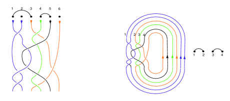
Figure 5. The closure of the tied braid $(I,\alpha)$ at left is the combinatoric tied link $(L,J)$ at right, where the four components are distinguished by different colors.

More precisely, if $k$ denotes the number of components of the link $\widehat{\alpha}$, or equivalently the number of cycles of the permutation $\pi_{\alpha}$, then $J$ is the set partition of $\bf k$ whose blocks are determined by those arcs of $I$ connecting strands belonging to different cycles of $\pi_{\alpha}$. For instance, in Figure 5 the arc (1,3) of $I$ connecting the blue and the red components, determines the arc (1,2) of $J$.

The extension of the Alexander and Markov theorems to combinatoric tied links, i.e. the characterization of the class of tied braids whose closures give the same combinatoric tied link, must take into account the behavior of the partition $I$ under closure of the tied braid $(I,\alpha)$. For this reason, before of stating the Alexander and Markov theorems for combinatoric tied links, we need to introduce the tools below.

Definition 9.

Let $I$, $K\in\mathsf{P}_{n}$ such that $K\preceq I$, let $m\leq n$ be the number of blocks of $K$ and ${\bf m}=\{1,\ldots,m\}$. We denote by $I/K$ the set partition of ${\bf m}$, whose blocks are the sets

$$(I/K)_{i}:=\{j\in{\bf m}\,:\,K_{j}\subseteq I_{i}\},$$

where the blocks $K_{j}$’s and $I_{i}$’s are taken standard indexed.

Example 3.

Let $I=\{\{1,2,5\},\{3,4\}\}$, $K=\{\{1,2\},\{3,4\},\{5\}\}$. Then $m=3$, $K_{1}=\{1,2\},\ K_{2}=\{3,4\},\ K_{3}=\{5\}$ and $I/K=\{\{1,3\},\{2\}\}$.

Proposition 4.

For $I\in\mathsf{P}_{n}$ with $k$ blocks, we have:

1. $I/I={\bf 1}_{k}$,

2. $I/{\bf 1}_{n}=I$.

Definition 10.

Let $K\in\mathsf{P}_{n}$ with $m$ blocks standard indexed $K_{1},\ldots,K_{m}$ and $J\in\mathsf{P}_{m}$ with $l$ blocks $J_{1},\dots,J_{l}$ standard indexed, too. We denote by $K\times J$ the set partition in $\mathsf{P}_{n}$ with $l$ blocks $(K\times J)_{i}$’s given by

$$(K\times J)_{i}=\cup_{j\in J_{i}}K_{j}.$$

Notice that $K\preceq K\times J$.

Example 4.

Let $K=\{\{1,2\},\{3,4\},\{5\}\}$, $m=3$, and $J:=\{\{1,3\},\{2\}\}$. Then $K\times J=\{\{1,2,5\},\{3,4\}\}$.

Notation 2.

Given a braid $\alpha\in B_{n}$, we denote by $K_{\alpha}\in\mathsf{P}_{n}$ the set partition whose blocks are the cycles of the permutation $\pi_{\alpha}$, including the 1–cycles.

Remark 3.

Recall that the closure of a classical braid $\alpha$ is a link whose components are in one–to–one correspondence with the cycles of the permutation $\pi_{\alpha}$. The standard indexation of the components of $\widehat{\alpha}$ is that obtained from the standard indexation of the cycles of $\pi_{\alpha}$.

Example 5.

Consider the braid $\alpha$ in Figure 5, left. We have $\pi_{\alpha}=(1,2)(3,6)$, so $K_{\alpha}=\{\{1,2\},\{3,6\},\{4\},\{5\}\}$. The four blocks correspond to the components of the link at right.

In order to distinguish a set partition $I\in\mathsf{P}_{n}$, associated to a tied braid $(I,\alpha)$, from a set partition $J\in\mathsf{P}_{k}$, associated to a tied link $(L,J)$, we shall call this last partition sc–partition (from set of components).

For $(I,\alpha)\in T\!B_{n}$ we define

$$\overline{I}_{\alpha}:=I\ast K_{\alpha}.$$ (33)

Proposition 5.

If the $k$–tied link $(L,J)$ is the closure of the tied braid $(I,\alpha)$, then the sc–partition $J$ is given by

$$J=\overline{I}_{\alpha}/K_{\alpha}.$$ (34)

Proof.

The number of blocks of $K_{\alpha}$, coincides with the number of components of $L$, i.e., $k$. If $\overline{I}$ has $m$ blocks, we have $m\leq k$; moreover, since $\overline{I}\preceq K_{\alpha}$, every block of $K_{\alpha}$ is contained in a block of $\overline{I}$. Therefore, $\overline{I}_{\alpha}/K_{\alpha}$ is a set partition of $\bf k$ having $m$ blocks. Now, by definition, the block $i$ of this set partition is

$$(\overline{I}_{\alpha}/K_{\alpha})_{i}=\{j\in{\bf k}\,;\,(K_{\alpha})_{j}\subseteq{\overline{I}}_{i}\}.$$

In other words, the elements of the set $(\overline{I}_{\alpha}/K_{\alpha})_{i}$ are the different blocks of $K_{\alpha}$, contained in the block $(\overline{I}_{\alpha})_{i}$. Therefore, an arc of the set partition $\overline{I}$, connecting two elements of $\bf n$ belonging to a same block of $K_{\alpha}$, does not determine an arc in $\overline{I}_{\alpha}/K_{\alpha}$. On the other hand, any arc of $\overline{I}$ connecting elements belonging to two different blocks of $K_{\alpha}$, determines an arc of $\overline{I}_{\alpha}/K_{\alpha}$. Therefore we conclude that $\overline{I}_{\alpha}/K_{\alpha}=J$. ∎

Example 6.

Fig. 6 shows at left a tied braid $(I,\alpha)$, where $I=\{\{1,3\},\{2\},\{4,5\},\{6\}\}$; in the middle the tied braid $(K_{\alpha},\alpha)$, where $K_{\alpha}=\{K_{1}=\{1,2\},K_{2}=\{3,6\},K_{3}=\{4\},K_{4}=\{5\}\}$, so that $k=4$; at right, the tied braid $(\overline{I},\alpha)$, where $\overline{I}=\{\{1,2,3,6\},\{4,5\}\}$. Observe that $\overline{I}$ is made by 2 blocks, the first containing the blocks $K_{1},K_{2}$ and the second containing the blocks $K_{3}$ and $K_{4}$ of $K_{\alpha}$. We thus have that the sc–partition $J\in\mathsf{P}_{4}$ is given by $\{\{1,2\},\{3,4\}\}$. Observe that the closure of $(I,\alpha)$ is the combinatoric tied link $(L,I_{2})$ shown in Fig. 4, right.

Figure 6.

We are ready now to prove the Alexander and Markov theorems in the context of combinatoric tied links.

Theorem 4 (Cf. [2, Theorem 3.5]).

Every combinatoric tied link can be obtained as closure of a tied braid. More precisely, if the link $L$ is the closure of the braid $\alpha$, then the combinatoric tied link $(L,J)$, up to a renumbering of the components, is the closure of the tied braid $(I,\alpha)$, where

$$I:=K_{\alpha}\times J.$$ (35)

Proof.

Let $(L,J)$ be a combinatoric tied link. Applying the Alexander theorem to the link $L$ we get a braid $\alpha$ whose closure is $L$. The standard indexed set partition $K_{\alpha}$ (see Remark 3) defines an ordering of the $k$ components of the closure of $\alpha$. On the other hand, the set partition $J$ is defined on the set of components ordered arbitrarily. By numbering the components of $L$, according to the standard ordering of the blocks of $K_{\alpha}$, we obtain from $J$ the partition $\tilde{J}$. Then the set partition $I$ of the tied braid $(I,\alpha)$ is obtained as $K_{\alpha}\times\tilde{J}$. ∎

Lemma 4.

Let $(I,\alpha)\in T\!B_{n}$. We have

$$\overline{I}_{\alpha}/K_{\alpha}=\overline{I}_{\alpha\sigma_{n}^{\pm 1}}/K_{\alpha\sigma_{n}^{\pm 1}}.$$ (36)

Proof.

Firstly note that the block of $K_{\alpha\sigma_{n}^{\pm 1}}$ containing $n$ also contains $n+1$; thus the set partitions $K_{\alpha}$ and $K_{\alpha\sigma_{n}^{\pm 1}}$ differ only in the bock that contains $n$. Secondly, we deduce then that $\overline{I}_{\alpha}$ and $\overline{I}_{\alpha\sigma_{n}^{\pm 1}}$ also differs only in the block that contains $n$. Thus, equation (36) follows. ∎

Theorem 5 (Cf. [2, Theorem 3.7]).

Denote by $\sim_{tM}$ the equivalence relation on $T\!B_{\infty}$ generated by the following replacements (or moves):

1. t–Stabilization: for all $(I,\alpha)\in TB_{n}$, we can do the following replacements:

   $$(I,\alpha)\quad\text{replaced by}\quad(I,\alpha)(\mu_{i,j},1)\quad\text{if}\quad i,j\quad\text{belong to the same cycle of}\quad\pi_{\alpha},$$

2. Commuting in $TB_{n}$: for all $(I_{1},\alpha),(I_{2},\beta)\in TB_{n}$, we can do the following replacement:

   $$(I_{1},\alpha)(I_{2},\beta)\quad\text{replaced by}\quad(I_{2},\beta)(I_{1},\alpha),$$

3. Stabilizations: for all $(I,\alpha)\in TB_{n}$, we can do the following replacements:

   $$(I,\alpha)\quad\text{replaced by}\quad(I,\alpha\sigma_{n})\quad\text{or}\quad(I,\alpha\sigma_{n}^{-1}).$$

Then, $(I,\alpha)\sim_{tM}(I,\beta)$ if and only if $\widehat{(I,\alpha)}\sim_{t}\widehat{(I^{\prime},\beta)}$.

Proof.

Firstly, we prove that the closure of a tied braid does not change under the replacement of M1, M2 and M3. Consider the replacement M1 on $(I,\alpha)$: according to Proposition 5, the set partition corresponding to the combinatoric tied link $\widehat{(I,\alpha)(\mu_{ij},1)}$ is given by

$$((I\ast\pi_{\alpha}(\mu_{i,j}))\ast K_{\alpha})/K_{\alpha}.$$

But $(I\ast\pi_{\alpha}(\mu_{i,j}))\ast K_{\alpha}=I\ast K_{\alpha}$, since $\pi_{\alpha}(\mu_{i,j})\preceq K_{\alpha}$, see (18). Thus, the closures of $(I,\alpha)$ and $(I,\alpha)(\mu_{ij},1)$ have the same sc–partition.

Secondly, we check that $(\widehat{\alpha\beta},J_{1}):=\widehat{(I_{1},\alpha)(I_{2},\beta)}$ and $(\widehat{\beta\alpha},J_{2}):=(I_{2},\beta)(I_{1},\alpha)$ are t–isotopic. Indeed, by Proposition 5:

$$J_{1}=((I_{1}\ast\pi_{\alpha}(I_{2}))\ast K_{\alpha\beta})/K_{\alpha\beta}\quad\text{and}\quad J_{2}=((I_{2}\ast\pi_{\beta}(I_{1}))\ast K_{\beta\alpha})/K_{\beta\alpha}.$$

Applying $\pi_{\beta}$ to the right member of the first equality, we get

$$(\pi_{\beta}(I_{1})\ast\pi_{\beta}(\pi_{\alpha}(I_{2}))\ast\pi_{\beta}(K_{\alpha\beta}))/\pi_{\beta}(K_{\alpha\beta}).$$

Notice now that $\pi_{\beta}(K_{\alpha\beta})=K_{\beta(\alpha\beta)\beta^{-1}}=K_{\beta\alpha}$. Then, applying now (19) to $\pi_{\beta\alpha}(I_{2})\ast K_{\beta\alpha}$ in the last expression, we obtain

$$\pi_{\beta}(I_{1})\ast(I_{2}\ast K_{\beta\alpha})/K_{\beta\alpha}=J_{2}.$$

Hence, setting $K:=K_{\alpha\beta}$ and $K^{\prime}:=K_{\beta\alpha}$, we have $J_{2}=w_{K,K^{\prime}}(J_{1})$, so that the sc–partitions $J_{1}$ and $J_{2}$ are iso–conjugate; this, together with the fact that $\widehat{\alpha\beta}$ and $\widehat{\beta\alpha}$ are isotopic, implies that $\widehat{(I_{1},\alpha)(I_{1},\beta)}$ and $\widehat{(I_{2},\beta)(I_{1},\alpha)}$ are t–isotopic.

Finally, notice now that Lemma 4 shows that the replacement M3 on $(I,\alpha)$ does not affect its closure.

To prove the statement in the other direction, let us suppose that two $t$–isotopic combinatoric tied links $(L,J)$ and $(L^{\prime},J^{\prime})$ are the closures of two tied braids $(I,\alpha)$ and $(I^{\prime},\alpha^{\prime})$. We have to prove that $(I,\alpha)\sim_{tM}(I^{\prime},\alpha^{\prime})$. We suppose that the ordering of the components in $J$ and $J^{\prime}$ corresponds, respectively, to that induced by $K_{\alpha}$ and $K_{\alpha^{\prime}}$.

Now, from the Markov theorem for classical links we know that the braids $\alpha$ and $\alpha^{\prime}$ are Markov equivalent, i.e., they are related by a sequence of replacements M2 and/or M3, where the set partitions are neglected. From (35), we have

$$I=K_{\alpha}\times J\quad\text{and}\quad I^{\prime}=K_{\alpha^{\prime}}\times J^{\prime}.$$

Observe also that $J$ and $J^{\prime}$ are set partitions iso–conjugate of $\bf{k}$, $k$ being the number of components of $L$ and $L^{\prime}$; we write $J^{\prime}=w(J)$, with $w\in S_{k}$. On the other hand, $K_{\alpha}$ and $K_{\alpha}^{\prime}$ are set partitions with $k$ blocks, respectively, of some $\bf{n}$ and $\bf{n^{\prime}}$. Since the M1 replacement does not affect the partition $K_{\alpha}$, we have to prove that the sequence of replacements M2 and/or M3 that transform $\alpha$ into $\alpha^{\prime}$, transforming by consequence the partition $K_{\alpha}$ into $K_{\alpha^{\prime}}$, induce the permutation $w$ above. Indeed, observe firstly that the set partition $K_{\alpha}$ is transformed step by step into a sequence of $r$ set partitions $K_{\alpha_{j}}$ (with $K_{\alpha_{1}}=K_{\alpha}$ and $K_{\alpha_{r}}=K_{\alpha^{\prime}}$) as long as $\alpha$ is transformed by moves M2 and/or M3 in the sequence $\alpha_{j}$, with $\alpha_{1}=\alpha$ and $\alpha_{r}=\alpha^{\prime}$. Secondly, notice that each partition $K_{\alpha_{j}}$ has $k$ blocks, and that for every pair $(j,j+1)$, writing for short $J$ for $K_{\alpha_{j}}$ and $J^{\prime}$ for $K_{\alpha_{j+1}}$, the permutation $w_{J,J^{\prime}}$ is the identity in the case of move M3, and different from the identity for the move M2. Since $L$ is the closure of $\alpha$ and $L^{\prime}$ is the closure of $\alpha^{\prime}$, the product of all $w_{J,J^{\prime}}$ coincides with the permutation $w_{L,L^{\prime}}$ operating the iso–conjugation between the combinatoric tied links $(L,J)$ and $(L^{\prime},J^{\prime})$.

∎

Theorems 4 and 5 imply the following

Corollary 1.

The mapping $\alpha\mapsto\widehat{\alpha}$ defines a bijection between $T\!B_{\infty}/\sim_{tM}$ and $\mathcal{L}^{t}/\sim_{t}$.

Example 7.

We show how the replacement M1 works. Consider the tied braids $(I,\alpha)$, in Figure 5, and $(I,\alpha)(\mu_{3,6},1)$, see Figure 7. Here $K_{\alpha}=\{\{1,2\},\{3,6\},\{4\},\{5\}\}$, so $\pi_{\alpha}(\mu_{3,6})=\mu_{3,6}$. Clearly, $\{\{3,6\}\}\preceq K_{\alpha}$.

Figure 7. $(I,\alpha)(\mu_{3,6},1)$ has the same closure as $(I,\alpha)$ shown in Fig. 5.

Example 8.

We show how the replacement M2 works. In Figure 8, we see two braids $\alpha\beta$ and $\beta\alpha$, with $K_{\alpha\beta}=\{\{1,3\},\{2\},\{4\}\}$ and $K_{\beta\alpha}=\{\{1\},\{2,4\},\{3\},\}$, so that $\pi_{\alpha\beta}=(1,3)$, $\pi_{\beta\alpha}=(2,4)$.

In Figure 9 we see the tied braids $(I_{1},\alpha)$ and $(I_{2},\beta)$, with $I_{1}=\{\{1,2\},\{3\},\{4\}\}$ and $I_{2}=\{\{1\},\{2,4\},\{3\}\}$. Consider now the closures of $(I_{1},\alpha)(I_{2},\beta)$ and $(I_{2},\beta)(I_{1},\alpha)$. These tied links are, respectively, $(\widehat{\alpha\beta},J_{1})$ and $(\widehat{\beta\alpha},J_{2})$, with the sc–partitions $J_{1}$ and $J_{2}$ given by

$$J_{1}=\overline{I}_{\alpha\beta}/K_{\alpha\beta}\quad\text{and}\quad J_{2}=\overline{I}_{\beta\alpha}/K_{\beta\alpha},$$

where

$$\overline{I}_{\alpha\beta}:=I_{1}\ast\pi_{\alpha}(I_{2})\ast K_{\alpha\beta}\quad\text{and}\quad\overline{I}_{\beta\alpha}:=I_{2}\ast\pi_{\beta}(I_{1})\ast K_{\beta\alpha}.$$

We have $\pi_{\alpha}=(1,4)(2,3)$ and $\pi_{\beta}=(1,2,3,4),$ so that:

$$\pi_{\alpha}(I_{2})=\{\{1,3\},\{2\},\{4\}\}\quad\text{and}\quad\pi_{\beta}(I_{1})=\{\{1\},\{2,3\},\{4\}\},$$

and

$$I_{1}\ast\pi_{\alpha}(I_{2})\ast K_{\alpha\beta}=\{\{1,2,3\},\{4\}\},$$

$$I_{2}\ast\pi_{\beta}(I_{1})\ast K_{\beta\alpha}=\{\{1\},\{2,3,4\}\}.$$

Finally,

$$J_{1}=\{\{1,2,3\},\{4\}\}/\{\{1,3\}_{1},\{2\}_{2},\{4\}_{3}\}=\{\{1,2\},\{3\}\},$$

and

$$J_{2}=\{\{1\},\{2,3,4\}\}/\{\{1\}_{1},\{2,4\}_{2},\{3\}_{3}\}=\{\{1\},\{2,3\}\}.$$

Observe now that $\pi_{\beta}(K_{\alpha\beta})=K_{\beta\alpha}$, and the corresponding permutation of $S_{3}$ is $w_{K,K^{\prime}}=(1,2,3)$. Indeed, $J_{2}=w_{K,K^{\prime}}(J_{1})$.

Figure 8. The tied braids $(K_{\alpha\beta},\alpha\beta)$ and $(K_{\beta\alpha},\beta\alpha)$.

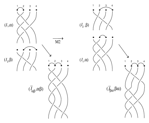
Figure 9. Here $I_{1}=\{\{1,2\}\}$ and $I_{2}=\{\{2,4\}\}$.

5. Invariant for singular links

In this section we define four families of invariants for singular links constructed by using the Jones recipe applied to the bt–algebra. We discuss also their definitions by skein relations. We start the section with a short recalling of the singular links theory.

5.1.

A singular link is a classical link admitting simple singular points. Thus, singular links are a generalization of classical links. Singular links can be studied trough singular braids: two singular links are isotopic if their respective singular braids are Markov equivalents; below we will be more precise.

Let $S\!B_{n}$ be the singular braid monoid defined independently by Baez [6], Birman [7] and Smolin [20]. $S\!B_{n}$ is defined by the elementary braid generators and their inverses $\sigma_{1}^{\pm 1},\ldots,\sigma_{n-1}^{\pm}$ and by the elementary singular braid generators $\tau_{1},\ldots,\tau_{n-1}$, which are subjected, besides the braid relations among the $\sigma_{i}$’s, to the following relations:

$$\begin{array}[]{rclcll}\tau_{i}\tau_{j}&=&\tau_{j}\tau_{i}\qquad\text{for $|i-j|>1$},\\ \sigma_{i}\tau_{i}&=&\tau_{i}\sigma_{i}\qquad\text{for all $i$},\\ \sigma_{i}\tau_{j}&=&\tau_{j}\sigma_{i}\qquad\text{for $|i-j|>1$},\\ \sigma_{i}\sigma_{j}\tau_{i}&=&\tau_{j}\sigma_{i}\sigma_{j}\qquad\text{for $|i-j|=1$}.\end{array}$$ (41)

This monoid is the basis for the Alexander theorem and for the Markov theorem for singular links, which are due, respectively, to J. Birman [7] and B. Gemein [11]. More precisely, we have the following theorem.

Theorem 6.

Every singular link can be obtained as closure of a singular braid and the closures of two singular braids are isotopic singular links if and only if the singular braids can be obtained one from the other by means of a finite number of replacements Ms1 and/or Ms2, where:

1. For all $\alpha,\beta\in SB_{n}$: $\alpha\beta\quad\text{is replaced by}\quad\beta\alpha,$

2. For all $\alpha\in SB_{n}$: $\alpha\quad\text{replaced by}\quad\alpha\sigma_{n}\quad\text{or}\quad\alpha\sigma_{n}^{-1}$.

5.2.

In this subsection we define invariants of singular links by using the Jones recipe applied to the bt–algebra, that is, the invariants are obtained essentially from the composition $\rho\circ\pi$, where $\pi$ is a representation of $SB_{n}$ in the bt–algebra and $\rho$ the trace on it, see Theorem 1.

Set $\mathsf{w}\,,\mathsf{x}$ and $\mathsf{y}\,$ three variable commuting among them and with $\mathsf{a}\,$ and $\mathsf{b}\,$. Define $\mathbb{L}$ as the field of rational functions $\mathbb{K}(\mathsf{a}\,,\mathsf{b}\,,\mathsf{x},\mathsf{y}\,,\mathsf{w}\,)$. From now on we work on the $\mathbb{L}$–algebra $\mathcal{E}_{n}(\mathsf{u}\,)\otimes_{\mathbb{K}}\mathbb{L}$ which is denoted again by $\mathcal{E}_{n}(\mathsf{u}\,)$, or simply by $\mathcal{E}_{n}.$

Proposition 6.

We have:

1. The mappings $\sigma_{i}\mapsto\mathsf{w}\,T_{i}$ and $\tau_{i}\mapsto\mathsf{x}+\mathsf{y}\,\mathsf{w}\,T_{i}$ define a monoid homomorphism, denoted by $\psi_{n,\mathsf{w}\,,\mathsf{x},\mathsf{y}\,}$, from $SB_{n}$ to $\mathcal{E}_{n}(u)$.

2. The mappings $\sigma_{i}\mapsto\mathsf{w}\,T_{i}$ and $\tau_{i}\mapsto\mathsf{x}E_{i}+\mathsf{y}\,\mathsf{w}\,E_{i}T_{i}$ define a monoid homomorphism, denoted by $\phi_{n,\mathsf{w}\,,\mathsf{x},\mathsf{y}\,}$, from $SB_{n}$ to $\mathcal{E}_{n}(u)$.

3. The mappings obtained by replacing $T_{i}$ with $V_{i}$ in items (1) and (2) (see Remark 1), define two monoid homomorphisms, denoted respectively $\psi^{\prime}_{n,\mathsf{w}\,,\mathsf{x},\mathsf{y}\,}$ and $\phi^{\prime}_{n,\mathsf{w}\,,\mathsf{x},\mathsf{y}\,}$, from $SB_{n}$ to $\mathcal{E}_{n}(\mathsf{v}\,)$.

Proof.

We need to verify that such mappings respect the defining relations of $SB_{n}$; this checking is a routine and is left to the reader. Notice that the second claim is a generalization of [3, Proposition 3]. ∎

Remark 4.

We will justify later the distinction apparently superfluous between $\psi_{n,\mathsf{w}\,,\mathsf{x},\mathsf{y}\,}$ and $\psi^{\prime}_{n,\mathsf{w}\,,\mathsf{x},\mathsf{y}\,}$ and between $\phi_{n,\mathsf{w}\,,\mathsf{x},\mathsf{y}\,}$ and $\phi^{\prime}_{n,\mathsf{w}\,,\mathsf{x},\mathsf{y}\,}$.

In order to derive invariants from the homomorphism of Proposition 6, we note that, due to replacement Ms2 of Theorem 6, $\mathsf{w}\,$ must satisfy (by using Theorem 2 and (11)):

$$\mathsf{w}\,^{2}=\frac{(\rho_{n}\circ\psi_{n,\mathsf{w}\,,\mathsf{x},\mathsf{y}\,})(\sigma_{n-1}^{-1})}{(\rho_{n}\circ\psi_{n,\mathsf{w}\,,\mathsf{x},\mathsf{y}\,})(\sigma_{n-1})}=\frac{(\rho_{n}\circ\phi_{n,\mathsf{w}\,,\mathsf{x},\mathsf{y}\,})(\sigma_{n-1}^{-1})}{(\rho_{n}\circ\phi_{n,\mathsf{w}\,,\mathsf{x},\mathsf{y}\,})(\sigma_{n-1})}=\frac{\mathsf{a}\,+(1-\mathsf{u}\,)\mathsf{b}\,}{\mathsf{a}\,\mathsf{u}\,}.$$ (42)

Now, set $\mathsf{c}\,:=\mathsf{w}\,^{2}.$ Then, for any singular link $L$, obtained as the closure of a singular braid $\omega\in SB_{n}$, we define:

$$\Psi_{\mathsf{x},\mathsf{y}\,}(L):=\left(\frac{1}{\mathsf{a}\,\sqrt{\mathsf{c}\,}}\right)^{n-1}(\rho_{n}\circ\psi_{n,\sqrt{\mathsf{c}\,},\mathsf{x},\mathsf{y}\,})(\omega),$$ (43)

and

$$\Phi_{\mathsf{x},\mathsf{y}\,}(L):=\left(\frac{1}{\mathsf{a}\,\sqrt{\mathsf{c}\,}}\right)^{n-1}(\rho_{n}\circ\phi_{n,\sqrt{\mathsf{c}\,},\mathsf{x},\mathsf{y}\,})(\omega).$$ (44)

Notice that $\Psi_{\mathsf{x},\mathsf{y}\,}$ and $\Phi_{\mathsf{x},\mathsf{y}\,}$ take values in $\mathbb{K}(\mathsf{a}\,,\mathsf{x},\mathsf{y}\,,\sqrt{\mathsf{c}\,})=\mathbb{K}(\mathsf{b}\,,\mathsf{x},\mathsf{y}\,,\sqrt{\mathsf{c}\,}).$

Theorem 7.

The functions $\Psi_{\mathsf{x},\mathsf{y}\,}$ and $\Phi_{\mathsf{x},\mathsf{y}\,}$ are ambient isotopy invariants of singular links.

Proof.

We have to prove that the functions $\Psi_{\mathsf{x},\mathsf{y}\,}$ and $\Phi_{\mathsf{x},\mathsf{y}\,}$ respect the moves Ms1 and Ms2 of Theorem 6. In fact, both functions respect Ms1 as consequence of rule (1) of Theorem 2, together with fact that $\psi_{n,\sqrt{\mathsf{c}\,},\mathsf{x},\mathsf{y}\,}$ and $\phi_{n,\sqrt{\mathsf{c}\,},\mathsf{x},\mathsf{y}\,}$ are homomorphisms.

We check now that $\Psi_{\mathsf{x},\mathsf{y}\,}(\widehat{\omega\sigma_{n}^{-1}})=\Psi_{\mathsf{x},\mathsf{y}\,}(\widehat{\omega})$, for $\omega\in SB_{n}$. We have:

$$(\rho_{n+1}\circ\psi_{n+1,\sqrt{\mathsf{c}\,},\mathsf{x},\mathsf{y}\,})(\omega\sigma_{n}^{-1})=\frac{1}{\sqrt{\mathsf{c}\,}}\rho_{n+1}(\omega T_{n}^{-1}) = \rho_{n}(\omega)\frac{\mathsf{a}\,+(\mathsf{u}\,^{-1}-1)\mathsf{b}\,+(\mathsf{u}\,^{-1}-1)\mathsf{a}\,}{\sqrt{\mathsf{c}\,}}$$

$$= \frac{(1-\mathsf{u}\,)\mathsf{b}\,+\mathsf{a}\,}{\mathsf{u}\,\sqrt{\mathsf{c}\,}}\rho_{n}(\omega);$$

hence, $(\rho_{n+1}\circ\psi_{n+1,\sqrt{\mathsf{c}\,},\mathsf{x},\mathsf{y}\,})(\omega\sigma_{n}^{-1})=\mathsf{a}\,\sqrt{\mathsf{c}\,}\rho_{n}(\omega)$. Then,

$$\Psi_{\mathsf{x},\mathsf{y}\,}(\widehat{\omega\sigma_{n}^{-1}})=\left(\frac{1}{\mathsf{a}\,\sqrt{\mathsf{c}\,}}\right)^{n}\mathsf{a}\,\sqrt{\mathsf{c}\,}\rho_{n}(\omega)=\Psi_{\mathsf{x},\mathsf{y}\,}(\widehat{\omega}).$$

In the same way we prove that $\Psi_{\mathsf{x},\mathsf{y}\,}(\widehat{\omega\sigma_{n}})=\Psi_{\mathsf{x},\mathsf{y}\,}(\widehat{\omega})$. The proof that $\Phi_{\mathsf{x},\mathsf{y}\,}$ respect Ms2 is analogous. ∎

The invariants $\Psi_{\mathsf{x},\mathsf{y}\,}$ and $\Phi_{\mathsf{x},\mathsf{y}\,}$ have, respectively, companions $\Psi_{\mathsf{x},\mathsf{y}\,}^{\prime}$ and $\Phi_{\mathsf{x},\mathsf{y}\,}^{\prime}$, which we define now. Firstly, notice that, because of (3) Proposition 6, we need in this case, by using Theorem 2:

$$\mathsf{w}\,^{2}=\frac{(\rho_{n}\circ\psi_{n,\mathsf{w}\,,\mathsf{x},\mathsf{y}\,}^{\prime})(\sigma_{n-1}^{-1})}{(\rho_{n}\circ\psi_{n,\mathsf{w}\,,\mathsf{x},\mathsf{y}\,}^{\prime})(\sigma_{n-1})}=\frac{(\rho_{n}\circ\phi_{n,\mathsf{w}\,,\mathsf{x},\mathsf{y}\,}^{\prime})(\sigma_{n-1}^{-1})}{(\rho_{n}\circ\phi_{n,\mathsf{w}\,,\mathsf{x},\mathsf{y}\,}^{\prime})(\sigma_{n-1})}=\frac{\mathsf{a}\,+(1-\mathsf{v}\,^{2})\mathsf{b}\,}{\mathsf{a}\,},$$ (45)

being $\rho_{n}(V_{n-1})=\mathsf{a}\,\mathsf{v}\,^{-1}$, see Eq. (15). Secondly, define $\mathsf{d}\,=\mathsf{w}\,^{2}$. Thus, for $L=\widehat{\omega}$, with $\omega\in SB_{n}$, we define:

$$\Psi_{\mathsf{x},\mathsf{y}\,}^{\prime}(L):=\left(\frac{\mathsf{v}\,}{\mathsf{a}\,\sqrt{\mathsf{d}\,}}\right)^{n-1}(\rho_{n}\circ\psi_{n,\sqrt{\mathsf{d}\,},\mathsf{x},\mathsf{y}\,}^{\prime})(\omega),$$ (46)

and

$$\Phi_{\mathsf{x},\mathsf{y}\,}^{\prime}(L):=\left(\frac{\mathsf{v}\,}{\mathsf{a}\,\sqrt{\mathsf{d}\,}}\right)^{n-1}(\rho_{n}\circ\phi_{n,\sqrt{\mathsf{d}\,},\mathsf{x},\mathsf{y}\,}^{\prime})(\omega).$$ (47)

Notice that $\Psi_{\mathsf{x},\mathsf{y}\,}^{\prime}$ and $\Phi_{\mathsf{x},\mathsf{y}\,}^{\prime}$ take values in $\mathbb{C}(\mathsf{v}\,,\mathsf{x},\mathsf{y}\,,\mathsf{a}\,,\sqrt{\mathsf{d}\,})=\mathbb{C}(\mathsf{v}\,,\mathsf{x},\mathsf{y}\,,\mathsf{b}\,,\sqrt{\mathsf{d}\,}).$

Theorem 8.

The functions $\Psi_{\mathsf{x},\mathsf{y}\,}^{\prime}$ and $\Phi_{\mathsf{x},\mathsf{y}\,}^{\prime}$ are ambient isotopy invariants of singular links.

Proof.

The same as the proof of Theorem 7. ∎

Remark 5.

Specializing $\mathsf{x}=\mathsf{y}\,=0$, the invariant $\Phi_{\mathsf{x},\mathsf{y}\,}$ evaluated on classical links coincides with the invariant $\overline{\Delta}$ defined in [3] and the invariant $\Phi_{\mathsf{x},\mathsf{y}\,}^{\prime}$ coincides with the invariant $\Theta$ defined in [9].

Remark 6.

Let $\omega\in SB_{n}$ and $s(\omega)$ the number its singularities. We have:

1. $(\rho_{n}\circ\phi_{n,\mathsf{w}\,,\mathsf{x},\mathsf{x}})(\omega)=\mathsf{x}^{s(\omega)}(\rho_{n}\circ\phi_{n,\mathsf{w}\,,1,1})(\omega)$. Then, $\Phi_{1,1}$ and $\Phi_{\mathsf{x},\mathsf{x}}$ are equivalent invariants.

2. $(\rho_{n}\circ\phi_{n,\mathsf{w}\,,\mathsf{x},\mathsf{y}\,})(\omega)=\mathsf{x}^{s(\omega)}(\rho_{n}\circ\phi_{n,\mathsf{w}\,,1,\mathsf{x}^{-1}\mathsf{y}\,})(\omega)$. Then, $\Phi_{\mathsf{x},\mathsf{y}\,}$ and $\Phi_{1,\mathsf{x}^{-1}\mathsf{y}\,}$ are equivalent invariants. In particular, it follows that $\Phi_{\mathsf{x},\mathsf{y}\,}$ is equivalent to $\Phi_{\tilde{\mathsf{x}},\tilde{\mathsf{y}}\,}$ if and only if $\mathsf{y}\,\mathsf{x}^{-1}=\tilde{\mathsf{y}}\,{\tilde{\mathsf{x}}}^{-1}$.

Proposition 7.

The polynomials $\Phi_{\mathsf{x},\mathsf{x}}$ and $\Phi_{\mathsf{x},\mathsf{y}\,}$ are not equivalent if $\mathsf{x}\not=\mathsf{y}\,$.

Proof.

To prove this proposition, it is sufficient to show a pair of non isotopic singular links which are are distinguished by $\Phi_{\mathsf{x},\mathsf{y}\,}$ but not by $\Phi_{\mathsf{x},\mathsf{x}}$. This in done in Section 8.2, Theorem 15. ∎

Remark 7.

We show now how the invariant $\Phi_{\mathsf{x},\mathsf{y}\,}$ generalizes the invariant $\bar{\Gamma}$ defined in [3]. Writing $\omega=\omega_{1}^{\epsilon_{1}}\cdots\omega_{m}^{\epsilon_{m}}$, where the $\omega_{i}$’s are the defining generators of $S\!B_{n}$, we define the exponent $\epsilon(\omega)$ of $\omega\in S\!B_{n}$ as

$$\epsilon(\omega):=c_{1}\epsilon_{1}+c_{2}\epsilon_{2}+\ldots+c_{m}\epsilon_{m},$$

where $c_{i}=1$ if $\omega_{i}=\sigma_{i}^{\pm 1}$, whereas $c_{i}=0$ if $\omega_{i}=\tau_{i}$. Then, the invariant $\Phi_{1,1/\mathsf{w}\,}$ can be written as follows:

$$\Phi_{1,1/\mathsf{w}\,}(L)=\left(\frac{1}{\mathsf{a}\,\sqrt{\mathsf{c}\,}}\right)^{n-1}\sqrt{\mathsf{c}\,}^{\;\epsilon(\omega)}(\rho_{n}\circ\phi_{n,1,1,1})(\omega),$$

where $L=\widehat{\omega}$. On the other hand, the invariant $\overline{\Gamma}$ can be written as:

$$\overline{\Gamma}(L)=\left(\frac{1}{\mathsf{a}\,\sqrt{\mathsf{c}\,}}\right)^{n-1}\sqrt{\mathsf{c}\,}^{\;\epsilon(\omega)+s(L)}(\rho_{n}\circ\phi_{n,1,1,1})(\omega).$$

Hence,

$$\overline{\Gamma}(L)=\sqrt{\mathsf{c}\,}^{\;s(L)}\Phi_{1,1/\mathsf{w}\,}(L),$$

where $L=\widehat{\omega}$ and $s(L)$ denotes the number of singular points of $L$. The exponent $s(L)$ is needed since in [3] and [14] the definition of the exponent $\omega$ takes $c_{i}=1$ when $\omega_{i}=\tau_{i}$.

6. Tied singular links

In this section we introduce the tied singular links and the combinatoric tied singular links. We introduce also the monoid of tied singular braids. The section ends by proving the Alexander and Markov theorems for tied singular links.

6.1.

We have two natural monoid homomorphisms from $SB_{n}$ onto $B_{n}$: the first one, denoted by $f$, maps $\sigma_{i}$ to $\sigma_{i}$ and $\tau_{i}$ to $\sigma_{i}$ and the second one, denoted by $f^{-}$, maps $\sigma_{i}$ to $\sigma_{i}$ and $\tau_{i}$ to $\sigma_{i}^{-1}$; notice that for every $\omega\in SB_{n}$, $(\pi\circ f)(\omega)=(\pi\circ f^{-})(\omega)$, where $\pi$, as in Subsection 1.2, denote the natural epimorphism from $B_{n}$ to $S_{n}$. Let $L$ be a singular link obtained as the closure of $\omega\in SB_{n}$; the closure, respectively, of $f(\omega)$ or $f^{-}(\omega)$ is the classical links obtained by replacing every singular point of $L$ by a positive crossing or, respectively, by a negative crossing. In terms of singular links, the replacement of a singular point by a positive or a negative crossing is called simple desingularization, and the singularity is said simply desingularized.

Definition 11.

The number of components of a singular link $L$, closure of a singular braid $\omega$, is the number of disjoint cycles of $(\pi\circ f)(\omega)$. In other words, the number of components of a singular link $L$ is the number of components of the classical link obtained by replacing every singular crossing with a positive (or negative) crossing in $L$.

Let $\mathcal{L}^{s}$ be the set of isotopy classes of singular links in $\mathbb{R}^{3}$, and $\mathcal{L}^{s}_{k,m}$ the set formed by those with $k$ components and $m$ singularities. Thus

$$\mathcal{L}^{s}=\coprod_{k>0,m\geq 0}\mathcal{L}^{s}_{k,m}.$$

The elements of $\mathcal{L}^{s}_{k,m}$ are called $(k,m)$–singular links.

Definition 12.

A tied singular link is a singular link with ties s.t. whenever the singular points are simply desingularized one obtains a tied link.

Definition 13.

Set $\mathcal{L}_{k,m}^{t,s}:=\mathcal{L}^{s}_{k,m}\times\mathsf{P}_{k}$. The elements of $\mathcal{L}_{k,m}^{t,s}$ are called $(k,m)$–combinatoric tied singular links. We call combinatoric tied singular links (for short cts–links) the elements of $\mathcal{L}^{t,s}$, where

$$\mathcal{L}^{t,s}:=\coprod_{k>0,m\geq 0}\mathcal{L}_{k,m}^{t,s}.$$

6.2.

The group $B_{n}$ is naturally a submonoid of $SB_{n}$ and the natural epimorphism $\pi:B_{n}\rightarrow S_{n}$, defined in Subsection 1.2, can be extend to $SB_{n}$ by mapping $\tau_{i}$ to $s_{i}$. We denote again this extension by $\pi$ and, consequently, we denote the image of $\tau_{i}$ by $\pi$ by $\pi_{\tau_{i}}$.

As before we define a monoid structure on the cartesian product $\mathsf{P}_{n}\times S\!B_{n}$, cf. (21), as follows: $(I,\alpha)(J,\beta)=(I\ast\pi_{\alpha}(J),\alpha\beta)$, where $I,J\in\mathsf{P}_{n}$ and $\alpha,\beta\in S\!B_{n}$; we denote this monoid by $\mathsf{P}_{n}\rtimes S\!B_{n}$.

Notice that the elements $\widetilde{\mu}_{i,j}$’s can be considered in $\mathsf{P}_{n}\rtimes S\!B_{n}$. We have:

$$(1,\tau_{k})(\mu_{i,j},1)=(\pi_{\tau_{k}}(\mu_{i,j}),\tau_{k})=(\pi_{\sigma_{k}}(\mu_{i,j}),1)(1,\tau_{k}).$$

Since Eq. (22) holds in $\mathsf{P}_{n}\rtimes S\!B_{n}$, we conclude that

$$\tau_{k}\widetilde{\mu}_{i,j}=\sigma_{k}\widetilde{\mu}_{i,j}\sigma_{k}^{-1}\tau_{k}.$$ (48)

Definition 14.

We define $T\!S\!B_{n}$ as the monoid presented by the braid generators $\sigma_{1}^{\pm 1},$ $\ldots,$ $\sigma_{n-1}^{\pm 1}$, the singular braid generators $\tau_{1},\ldots,\tau_{n-1}$ of $S\!B_{n}$ and the ties generators $\eta_{1},\ldots,\eta_{n-1}$ of $T\!B_{n}$, subject to the following relations: the defining relations of $SB_{n}$, the defining relations of $T\!B_{n}$ and the relations:

$$\tau_{i}\eta_{i} = \eta_{i}\tau_{i}\qquad\text{ for all $i$},$$ (49)

$$\tau_{i}\eta_{j} = \eta_{j}\tau_{i}\qquad\text{for $|i-j|>1$},$$ (50)

$$\eta_{i}\tau_{j}\tau_{i} = \tau_{j}\tau_{i}\eta_{j}\qquad\text{ for $|i-j|=1$},$$ (51)

$$\eta_{i}\eta_{j}\tau_{i} = \eta_{j}\tau_{i}\eta_{j}\quad=\quad\tau_{i}\eta_{i}\eta_{j}\qquad\text{ for $|i-j|=1$},$$ (52)

$$\eta_{i}\tau_{j}\sigma_{i} = \tau_{j}\sigma_{i}\eta_{j}\qquad\text{ for $|i-j|=1$},$$ (53)

$$\eta_{i}\sigma_{j}\tau_{i} = \sigma_{j}\tau_{i}\eta_{j}\qquad\text{ for $|i-j|=1$},$$ (54)

$$\tau_{i}\eta_{j} = \sigma_{i}\eta_{j}\sigma_{i}^{-1}\tau_{i}\qquad\text{ for $|i-j|=1$}.$$ (55)

Remark 8.

Note that, by allowing $i,j$ take every possibility in (55), the relations (49) and (50) are included in (55). Further, relation (55) can be written, equivalently, by exchanging $\sigma_{i}$ with $\sigma_{i}^{-1}$.

Theorem 9.

The monoids $T\!S\!B_{n}$ and $\mathsf{P}_{n}\rtimes S\!B_{n}$ are isomorphic.

Proof.

(Analogous to proof of Theorem 3) It is a routine to check that the mappings $\sigma_{i}\mapsto\sigma_{i}$, $\tau_{i}\mapsto\tau_{i}$ and $\eta_{i}\mapsto\widetilde{\mu}_{i,i+1}$ define a morphism $\phi$ from $T\!S\!B_{n}$ to $\mathsf{P}_{n}\rtimes S\!B_{n}$. Now, arguing as in Lemma 1, we obtain that $\mathsf{P}_{n}\rtimes SB_{n}$ is generated by $\widetilde{\mu}_{1,2},\ldots,\widetilde{\mu}_{n-1,n}$, $\sigma_{1}^{\pm 1},\ldots,\sigma_{n-1}^{\pm 1}$, $\tau_{1},\ldots,\tau_{n-1}$; then it follows that $\phi$ is an epimorphism. The injectivity of $\phi$ is proved as the injectivity in Theorem 20; therefore it is enough to prove that every element $\mathsf{P}_{n}\rtimes SB_{n}$ has the decomposition $\eta_{I}\beta$, where $I\in\mathsf{P}_{n}$ and $\beta\in SB_{n}$; in the present situation such decomposition is obtained by combining (4) of Lemma 2 with (48), cf. Proposition 2. ∎

Definition 15.

The closure of a tied singular braid, i.e. an element of $T\!S\!B_{n}\simeq\mathsf{P}_{n}\rtimes S\!B_{n}$, is defined in the same way as the closure of a tied braid (see Definition 8). I.e., given a tied singular braid $(J,\omega)$, its closure $\widehat{(J,\omega)}$ is equal to $(\widehat{\omega},I)$, with $I=I_{f(\omega)}$, where $I_{f(\omega)}$ is the set partition defined by the closure of the tied braid $(J,f(\omega))$.

6.3.

We are now in position to establish and to prove the Alexander and Markov theorem for cts–links.

Theorem 10 (Alexander theorem for cts–links).

Every cts–link can be obtained as the closure of a tied singular braid. More precisely, given the cts–link $(L,J)$, where $L$ is the closure of the singular braid $\omega$, then $(L,J)$, up to a renumbering the components, is the closure of the tied singular braid $(I,\omega)$, where $I$ is defined by

$$I=K_{f(\omega)}\times J.$$

Proof.

Set $(L,J)\in\mathcal{L}^{s}_{k,m}\times\mathsf{P}_{k}$. Let $\omega=\omega_{1}\cdots\omega_{l}\in SB_{n}$ whose closure is $L$, where the $\omega_{i}$’s are the defining generators of $SB_{n}$. Let $L^{\prime}$ be the classical link obtained as the closure of $f(\omega)$; so $k$ is the number of components of $L^{\prime}$. Now, from Theorem 4 applied to the combinatoric tied link $(L^{\prime},J)$, we have that, up to the renumbering the components, it is the closure of the tied braid $(I,f(\omega))$, where $I=K_{f(\omega)}\times J$. Thus, it follows that $(L,J)$ is the closure of the tied singular braid $(I,\omega)$. ∎

Theorem 11 (Markov theorem for cts–links).

Two tied singular braids yield the same cts–link if and only if they are $\sim_{Mts}$–equivalent, i.e. one is obtained from the other by using the replacements Mts1/Mts2/and or Mts3 below.

1. t–Stabilization: for all $(I,\alpha)\in TSB_{n}$, we can do the following replacements:

   $$(I,\alpha)\quad\text{replaced by}\quad(I,\alpha)(\mu_{i,j},1)\quad\text{if}\quad i,j\quad\text{belong to the same cycle of}\quad\pi_{\alpha},$$

2. Commuting in $TSB_{n}$: for all $(I_{1},\alpha),(I_{2},\beta)\in TB_{n}$, we can do the following replacement:

   $$(I_{1},\alpha)(I_{2},\beta)\quad\text{replaced by}\quad(I_{2},\beta)(I_{1},\alpha),$$

3. Stabilizations: for all $(I,\alpha)\in TSB_{n}$, we can do the following replacements:

   $$(I,\alpha)\quad\text{replaced by}\quad(I,\alpha\sigma_{n})\quad\text{or}\quad(I,\alpha\sigma_{n}^{-1}).$$

Proof.

Let $(I,\omega)\in TSB_{n}$; according to Definition 15, the set partition determined by $\widehat{(I,\omega)}$ is the set partition determined by $\widehat{(I,f(\omega))}$. Thus, the verification that the replacements Mts1, Mts2 and/or Mts3 do not alter the closure of a singular tied braid results in a repetition of the verification that the Markov replacements of Theorem 5 do not affect the closure of a combinatoric tied braid.

In the other direction we use again the fact that, by definition, the set partition determined by $\widehat{(I,\omega)}$ is equal to the set partition determined by $\widehat{(I,f(\omega))}$. Then the proof follows from those of Theorem 6 and Theorem 5.

∎

7. Invariants of cts–links

We will extend the invariants of Theorems 7 and 8 to invariants for cts–links. Thanks to Theorems 10 and 11, we deduce that the definitions of these extensions are reduced to extend the domain of the maps $\phi_{n,\mathsf{w}\,,\mathsf{x},\mathsf{y}\,}$ and $\psi_{n,\mathsf{w}\,,\mathsf{x},\mathsf{y}\,}$ to $TSB_{n}$. More generally, the next proposition extends the homomorphisms of Proposition 6.

Proposition 8.

For all $n$, the domain of definition of the morphisms $\phi_{n,\mathsf{w}\,,\mathsf{x},\mathsf{y}\,}$ and $\psi_{n,\mathsf{w}\,,\mathsf{x},\mathsf{y}\,}$ can be extended to $T\!S\!B_{n}$, by mapping $\eta_{i}$ to $E_{i}$. We shall keep, respectively, the same notations $\phi_{n,\mathsf{w}\,,\mathsf{x},\mathsf{y}\,}$ and $\psi_{n,\mathsf{w}\,,\mathsf{x},\mathsf{y}\,}$ for these extensions.

Proof.

The proof follows by checking that these extensions respect the relations (49)–(55); these checkings are straightforward. For instance, we now verify Relation (53). Set $\phi_{n}=\phi_{n,\mathsf{w}\,,\mathsf{x},\mathsf{y}\,}$ and suppose $|i-j|=1$. Since $E_{i}E_{j}$ commutes with $T_{i}$ and $T_{j}$, we have: $\phi_{n}(\eta_{i})\phi_{n}(\tau_{j})\phi_{n}(\sigma_{i})=E_{i}(\mathsf{x}E_{j}+\mathsf{y}\,\mathsf{w}\,E_{j}T_{j})\mathsf{w}\,T_{i}=(\mathsf{x}E_{j}+\mathsf{y}\,\mathsf{w}\,E_{j}T_{j})\mathsf{w}\,T_{i}E_{i}$, from (7). So:

$$\phi_{n}(\eta_{i})\phi_{n}(\tau_{j})\phi_{n}(\sigma_{i})=(\mathsf{x}E_{j}+\mathsf{y}\,\mathsf{w}\,E_{j}T_{j})\mathsf{w}\,T_{i}E_{i}=\phi_{n}(\tau_{j})\phi_{n}(\sigma_{i})\phi_{n}(\eta_{j}).$$

∎

Remark 9.

Also the domain of the homomorphisms (3) of Proposition 6 can be extended to $TSB_{n}$. As in the proposition above, we keep the same notations, that is $\psi_{n,\mathsf{w}\,,\mathsf{x},\mathsf{y}\,}^{\prime}$ and $\phi_{n,\mathsf{w}\,,\mathsf{x},\mathsf{y}\,}^{\prime}$, for these extensions.

The invariants $\Psi_{\mathsf{x},\mathsf{y}\,}$ and $\Phi_{\mathsf{x},\mathsf{y}\,}$ for singular links can be extended to invariants for tied singular links simply by taking, respectively, in the definition of (43) and (44), the extensions $\psi_{n,\sqrt{\mathsf{c}\,},\mathsf{x},\mathsf{y}\,}$ and $\phi_{n,\sqrt{\mathsf{c}\,},\mathsf{x},\mathsf{y}\,}$ to $TSB_{n}$ of Proposition 8; we denote again these invariants for cts–links by $\Psi_{\mathsf{x},\mathsf{y}\,}$ and $\Phi_{\mathsf{x},\mathsf{y}\,}$. Repeating the argument on the invariants of Theorem 8, we obtain invariants for cts–links again keeping the notation $\Psi_{\mathsf{x},\mathsf{y}\,}^{\prime}$ and $\Phi_{\mathsf{x},\mathsf{y}\,}^{\prime}$.

7.1. Skein rules

In this section we will define the invariants $\Phi_{\mathsf{x},\mathsf{y}\,}$ and $\Psi_{\mathsf{x},\mathsf{y}\,}$ by skein rule and desingularization. Recall now that both $\Phi_{\mathsf{x},\mathsf{y}\,}$ and $\Psi_{\mathsf{x},\mathsf{y}\,}$ are extensions of $\mathcal{F}$ to singular links, therefore the skein rules of them must contain the skein rules of $\mathcal{F}$; so, in particular, the defining skein relations of $\mathcal{F}$ will be reformulated in the context of cts–links. Recall that in a cts–link $(L,J)$, the components of $L$ are numbered and the parts of the set partition $J$ are standardly indexed. Now we need to introduce the notations below.

Notation 3.

Consider a generic diagram of a cts–link $(L,J)$, suppose that $J$ has blocks $J_{1},\ldots,J_{m}$ and $L$ has a positive crossing such that the components of this crossing belong to two blocks $J_{i}$ and $J_{k}$ ($i\leq k$) of $J$. We shall denote by:

1. $(L_{+}^{i,k},J)$ the link $(L,J)$;

2. $(L_{-}^{i,k},J)$ the same as the previous, but the positive crossing is replaced by a negative crossing;

3. $(L_{\times}^{i,k},J)$ the same as above, but now the crossing is replaced by a singular crossing;

4. $(L_{+}^{i,i},J^{\prime})$ as $(L_{+}^{i,k},J)$, where $J^{\prime}$ is the set partition obtained from $J$ by considering the union of $J_{i}$ and $J_{k}$ as a unique part;

5. $(L_{-}^{i,i},J^{\prime})$ the same as the previous, but the positive crossing is replaced by a negative crossing;

6. $(L_{\times}^{i,i},J^{\prime})$ the same as the previous, but the crossing is now a singular crossing;

7. $(L_{0}^{i,i},J^{\prime\prime})$ the initial link, where the crossing strands are replaced by two non crossing strands and the parts containing the components crossing merge in a unique part in $J^{\prime\prime}$.

Remark 10.

Let us suppose $J\in\mathsf{P}_{n}$ has $m$ blocks, we have:

1. If the crossing components belong to different blocks, then $J^{\prime}$ is in $\mathsf{P}_{n}$ and has $(m-1)$ blocks. Moreover, the two crossing components merge in a unique component in $L_{0}^{i,i}$, therefore $J^{\prime\prime}\in\mathsf{P}_{n-1}$.

2. In the case that the crossing components belong to a same block of the set partition, we have $J^{\prime}=J$. However, observe that the two crossing strands may belong to two different components or to a same component. In the first case, the two different components merge in a unique component in $L_{0}^{i,i}$, then $J^{\prime\prime}\in\mathsf{P}_{n-1}$ and has $m$ parts; in the second case, the component splits in two components, still belonging to the same $i$–th block, thus, $J^{\prime\prime}\in\mathsf{P}_{n+1}$.

3. Observe that, in order to define the skein rules, neither the total number of components nor the total number of parts of the partition is relevant. Therefore we shall use the notation $(i,k)$ for both cases $J_{i}=J_{k}$ and $J_{i}\not=J_{k}$.

Before of stating the main theorems of this section we introduce the notation ${\rm I}(L,J)$ to indicate the value of the invariant $\rm I$ on the cts–link $(L,J)$.

Theorem 12.

The invariant $\Phi_{\mathsf{x},\mathsf{y}\,}$ of singular tied links is defined uniquely by four rules. More precisely, the values of $\Phi_{\mathsf{x},\mathsf{y}\,}$ on a cts–link $(L,J)$, with $n$ components, is determined through the rules:

1. The value of $\Phi_{\mathsf{x},\mathsf{y}\,}$ is equal to 1 on the unknotted circle.

2. $$\Phi_{\mathsf{x},\mathsf{y}\,}(L\sqcup O,\iota_{n}(J))=\frac{1}{\mathsf{a}\,\sqrt{\mathsf{c}\,}}\Phi_{\mathsf{x},\mathsf{y}\,}(L,J),$$

   where $\iota_{n}$ is the natural inclusion of $\mathsf{P}_{n}$ into $\mathsf{P}_{n+1}$ (see Definition 2).

3. Skein rule.

   $$\frac{1}{\sqrt{\mathsf{c}}\,}\Phi_{\mathsf{x},\mathsf{y}\,}(L_{+}^{i,k},J)+\sqrt{\mathsf{c}}\,\Phi_{\mathsf{x},\mathsf{y}\,}(L_{-}^{i,k},J)=\frac{1}{\sqrt{\mathsf{c}}\,}(1-\mathsf{u}\,^{-1})\Phi_{\mathsf{x},\mathsf{y}\,}(L_{+}^{i,i},J^{\prime})+(1-\mathsf{u}\,^{-1})\Phi_{\mathsf{x},\mathsf{y}\,}(L_{0}^{i,i},J^{\prime\prime}).$$

4. Desingularization.

   $$\Phi_{\mathsf{x},\mathsf{y}\,}(L_{\times}^{i,k},J)=\mathsf{x}\Phi_{\mathsf{x},\mathsf{y}\,}(L_{0}^{i,i},J^{\prime\prime})+\mathsf{y}\,\Phi_{\mathsf{x},\mathsf{y}\,}(L_{+}^{i,i},J^{\prime}).$$

Theorem 13.

The invariant $\Psi_{\mathsf{x},\mathsf{y}\,}$ is defined by the same rules I–III as $\Phi_{\mathsf{x},\mathsf{y}\,}$ in Theorem 12 but the desingularization rule IV is replaced by

1. $$\Psi_{\mathsf{x},\mathsf{y}\,}(L_{\times}^{i,k},J)=\mathsf{x}\Psi_{\mathsf{x},\mathsf{y}\,}(L_{0}^{i,i},J^{\prime\prime})+\mathsf{y}\,\Psi_{\mathsf{x},\mathsf{y}\,}(L_{+}^{i,k},J).$$

Proof of Theorems 12 and 13.

For non singular combinatoric tied links, both $\Phi_{\mathsf{x},\mathsf{y}\,}$ and $\Psi_{\mathsf{x},\mathsf{y}\,}$ coincide with the polynomial $\mathcal{F}$ for tied links, defined in [2, Theorem 2.1]; indeed, rules I–III are exactly the skein rules I–III of $\mathcal{F}$, under the replacements $\mathsf{u}\,\rightarrow u$, $\sqrt{\mathsf{c}}\,\rightarrow w$, $\mathsf{a}\,\rightarrow z$, and observing that the translation between the notations of tied links [2, Fig. 3] and cts–links of Notation 3 is as follows: the tied link $L_{\pm}$ with a positive/negative crossing corresponds to the cts–link $(L_{\pm}^{i,k},J)$; $L_{\pm,\sim}$ corresponds to $(L_{\pm}^{i,i},J^{\prime})$ and $L_{0,\sim}$ corresponds to $(L_{0}^{i,i},J^{\prime\prime})$. To conclude the the proof, it remains to verify the desingularization rules IV and IV’. Suppose that the cts–link $(L_{\times}^{i,j},J)$ has only one singularitiy, and that it is the closure of the singular tied braid $\omega=\alpha\tau_{i}\beta$, with $\alpha,\beta\in T\!B_{n}$. In order to calculate $\Phi_{\mathsf{x},\mathsf{y}\,}$ (respectively $\Psi_{\mathsf{x},\mathsf{y}\,}$), we have to calculate the trace of the image of $\omega$ in the bt–algebra. By using Proposition 6, we obtain that the image of $\omega$ splits into a linear combination of two elements, precisely

$$\mathsf{x}(\phi_{n,\mathsf{w}\,,\mathsf{x},\mathsf{y}\,}(\alpha)E_{i}\phi_{n,\mathsf{w}\,,\mathsf{x},\mathsf{y}\,}(\beta))+\mathsf{y}\,(\phi_{n,\mathsf{w}\,,\mathsf{x},\mathsf{y}\,}(\alpha)\mathsf{w}\,E_{i}T_{i}\phi_{n,\mathsf{w}\,,\mathsf{x},\mathsf{y}\,}(\beta)),$$

(respectively, $\mathsf{x}(\psi_{n,\mathsf{w}\,,\mathsf{x},\mathsf{y}\,}(\alpha)\psi_{n,\mathsf{w}\,,\mathsf{x},\mathsf{y}\,}(\beta))+\mathsf{y}\,(\psi_{n,\mathsf{w}\,,\mathsf{x},\mathsf{y}\,}(\alpha)\mathsf{w}\,T_{i}\psi_{n,\mathsf{w}\,,\mathsf{x},\mathsf{y}\,}(\beta))).$ These elements are the images in the bt–algebra of $\alpha\eta_{i}\beta$ and $\alpha\sigma_{i}\eta_{i}\beta$ (respectively, of $\alpha\beta$ and $\alpha\sigma_{i}\beta$), whose closures give the cts–links $(L_{0}^{i,i},J^{\prime\prime})$ and $(L_{+}^{i,i},J^{\prime})$, (respectively the cts–links $(L_{0}^{i,i},J^{\prime\prime})$ and $(L_{+}^{i,j},J)$. The desingularization rules IV and IV’ then follow from the linearity of the trace together with the defining formulae (44) and (43). If the number of singularities of the cts–link is higher, say $m$, the argument remains the same, i.e., by comparing the result of the desingularization rule IV (or IV’) to all $m$ singularities of the link (result that is independent from the order on which they are applied) and the image in the bt–algebra of the corresponding singular braid with $m$ elements $\tau_{i}$, according to the respective map of Proposition 6. ∎

The analogous of Theorems 12 and 13 are as follows.

Theorem 14.

1. The invariant $\Phi^{\prime}_{\mathsf{x},\mathsf{y}\,}$ is defined by the same rules I, II and IV as $\Phi_{\mathsf{x},\mathsf{y}\,}$ in Theorem 12 but the skein rule III is replaced now by:

   1. Skein rule,

      $$\frac{1}{\sqrt{\mathsf{d}}\,}\Phi^{\prime}_{\mathsf{x},\mathsf{y}\,}(L_{+}^{i,k},J)+\sqrt{\mathsf{d}}\,\Phi^{\prime}_{\mathsf{x},\mathsf{y}\,}(L_{-}^{i,k},J)=(\mathsf{v}\,-\mathsf{v}\,^{-1})\Phi^{\prime}_{\mathsf{x},\mathsf{y}\,}(L_{0}^{i,i},J^{\prime\prime}).$$

2. The invariant $\Psi^{\prime}_{\mathsf{x},\mathsf{y}\,}$ is defined by the same rules I, II and IV’ as $\Psi_{\mathsf{x},\mathsf{y}\,}$ in Theorem 13 but the skein rule III is replaced by the III’ above in which $\Phi^{\prime}$ is replaced by $\Psi^{\prime}$.

Proof.

For non singular combinatoric tied links, both $\Phi^{\prime}_{\mathsf{x},\mathsf{y}\,}$ and $\Psi^{\prime}_{\mathsf{x},\mathsf{y}\,}$ coincide with the polynomial $\overline{\Theta}$ for tied links, defined in [9]; indeed, rules I–III’ are exactly the skein rules of $\overline{\Theta}$, under the replacements $\mathsf{v}\,\rightarrow q$, $\mathsf{c}\,\rightarrow\lambda$, $\mathsf{a}\,\rightarrow z$. After, the proof proceeds as the proof of Theorems 12 and 13. ∎

Remark 11.

1. The desingularization rules IV and IV’ coincide when the components crossing at the singular point belong to the same part of the partition. This implies that $\Phi_{\mathsf{x},\mathsf{y}\,}=\Psi_{\mathsf{x},\mathsf{y}\,}$ for knots and cts–links having a set partition with a sole part.

2. The invariants $\Phi$ and $\Phi^{\prime}$ have the same desingularization rule IV, while he invariants $\Psi$ and $\Psi^{\prime}$ have the same desingularization rule IV’.

3. From the desingularization rules IV and IV’ it follows that the invariant polynomial $\Phi_{\mathsf{x},\mathsf{y}\,}$ as well as the other invariants $\Phi^{\prime}_{\mathsf{x},\mathsf{y}\,},\Psi_{\mathsf{x},\mathsf{y}\,}$ and $\Psi^{\prime}_{\mathsf{x},\mathsf{y}\,}$, when evaluated on a cts–link ${\rm{S}}$ with $m$ singularities, is homogeneous of degree $m$ in the variables $\mathsf{x},\mathsf{y}\,$ (see also Remark 6):

   $$\Phi_{\mathsf{x},\mathsf{y}\,}({\rm{S}})=\mathsf{x}^{m}\Phi_{1,\mathsf{y}\,/\mathsf{x}}({\rm{S}}).$$

8. Comparison of invariants

In this section we compare the invariants here introduced with each other and with the Paris–Rabenda invariant [18]. The comparison of our invariants is done on pairs of singular links constructed from pairs of non isotopic classical links not distinguished by the Hompflyt polynomial; these pairs are taken from [8].

8.1. Notation and some elementary facts.

In what follows we will denote by:

1. $P$ the Homflypt polynomial for classical links,

2. $\mathcal{F}$ the polynomial for tied links,

3. $\mathcal{F}^{\prime}$ the polynomial for tied links $\overline{\Theta}$ (see [9]) constructed by the Jones recipe as $\mathcal{F}$ but using the presentation of the bt–algebra $\mathcal{E}_{n}(\mathsf{v}\,)$ (see Remark 1) instead of the presentation $\mathcal{E}_{n}(\mathsf{u}\,)$,

4. ${\rm{I}}_{PR}$ the polynomial for singular links due to Paris and Rabenda [18],

5. When we say that two non isotopic (singular) links with $n$ components $L$ and $L^{\prime}$ are distinguished by an invariant ${\rm{I}}$ for tied (singular) links, we mean that ${\rm{I}}(L,{\bf 1}_{n})\not={\rm{I}}(L^{\prime},{\bf 1}_{n})$. In the same way we did in [4, Subsection 2.3].

The following proposition comes out by an appropriate renaming of the variables.

Proposition 9.

1. If $L$ is a classical link, then ${\rm{I}}_{PR}(L)=P(L)$,

2. If $L$ is a classical link and $I$ the set partition with a unique block, then:

   $$\mathcal{F}(L,I)=\mathcal{F}^{\prime}(L,I)=P(L),$$

3. If $L$ is a non singular tied link with $n$ components, then:

   $$\Phi_{\mathsf{x},\mathsf{y}\,}(L,{\bf 1}_{n})=\Psi_{\mathsf{x},\mathsf{y}\,}(L,{\bf 1}_{n})=\mathcal{F}(L,{\bf 1}_{n}),$$

4. If $L$ is a non singular tied link with $n$ components, then:

   $$\Phi_{\mathsf{x},\mathsf{y}\,}^{\prime}(L,{\bf 1}_{n})=\Psi_{\mathsf{x},\mathsf{y}\,}^{\prime}(L,{\bf 1}_{n})=\mathcal{F}^{\prime}(L,{\bf 1}_{n}),$$

5. If $L$ is a singular classical link and $I$ the set partition with a unique block, then

   $$\Psi_{\mathsf{x},\mathsf{y}\,}(L,I)=\Psi^{\prime}_{\mathsf{x},\mathsf{y}\,}(L,I)=\Phi_{\mathsf{x},\mathsf{y}\,}(L,I)=\Phi^{\prime}_{\mathsf{x},\mathsf{y}\,}(L,I)={\rm{I}}_{PR}(L).$$

8.2. Differences between $\Phi_{\mathsf{x},\mathsf{y}\,}$ and $\Psi_{\mathsf{x},\mathsf{y}\,}$

In this section we analyze some properties of $\Phi_{\mathsf{x},\mathsf{y}\,}$ and $\Psi_{\mathsf{x},\mathsf{y}\,}$. By Remark 11 (2), the next proposition and Theorem 15 hold identically if $\Phi_{\mathsf{x},\mathsf{y}\,}$ and $\Psi_{\mathsf{x},\mathsf{y}\,}$ are replaced, respectively, by $\Phi^{\prime}_{\mathsf{x},\mathsf{y}\,}$ and $\Psi^{\prime}_{\mathsf{x},\mathsf{y}\,}$.

The following proposition shows that $\Psi_{\mathsf{x},\mathsf{y}\,}$ is more powerful than $\Phi_{\mathsf{x},\mathsf{y}\,}$ on cts–links.

Take any classical singular link ${\rm{S}}$ with $n$ components, having at least one singularity involving two distinct components $i$ and $j$. Consider the cts–links $({\rm{S}}_{\times}^{i,j},{\bf 1}_{n})$ and $({\rm{S}}_{\times}^{i,i},\{\{i,j\}\})$.

Proposition 10.

$$\Psi_{\mathsf{x},\mathsf{y}\,}({\rm{S}}_{\times}^{i,j},{\bf 1}_{n})\not=\Psi_{\mathsf{x},\mathsf{y}\,}({\rm{S}}_{\times}^{i,i},\{\{i,j\}\}),$$

while

$$\Phi_{\mathsf{x},\mathsf{y}\,}({\rm{S}}_{\times}^{i,j},{\bf 1}_{n})=\Phi_{\mathsf{x},\mathsf{y}\,}({\rm{S}}_{\times}^{i,i},\{\{i,j\}\}).$$

Proof.

We have, respectively, by rules IV’ and IV:

$$\Psi_{\mathsf{x},\mathsf{y}\,}({\rm{S}}_{\times}^{i,j},{\bf 1}_{n})=\mathsf{x}\ \Psi_{\mathsf{x},\mathsf{y}\,}({\rm{S}}_{0}^{i,i},{\bf 1}_{n-1})+\mathsf{y}\,\ \Psi_{\mathsf{x},\mathsf{y}\,}({\rm{S}}_{+}^{i,j},{\bf 1}_{n}),$$

$$\Psi_{\mathsf{x},\mathsf{y}\,}({\rm{S}}_{\times}^{i,i},\{\{i,j\}\})=\mathsf{x}\ \Psi_{\mathsf{x},\mathsf{y}\,}({\rm{S}}_{0}^{i,i},{\bf 1}_{n-1})+\mathsf{y}\,\ \Psi_{\mathsf{x},\mathsf{y}\,}({\rm{S}}_{+}^{i,i},\{\{i,j\}\});$$

while

$$\Phi_{\mathsf{x},\mathsf{y}\,}({\rm{S}}_{\times}^{i,j},{\bf 1}_{n})=\Phi_{\mathsf{x},\mathsf{y}\,}({\rm{S}}_{\times}^{i,i},\{\{i,j\}\})=\mathsf{x}\ \Phi_{\mathsf{x},\mathsf{y}\,}({\rm{S}}_{0}^{i,i},{\bf 1}_{n-1})+\mathsf{y}\,\ \Phi_{\mathsf{x},\mathsf{y}\,}({\rm{S}}_{+}^{i,i},\{\{i,j\}\}).$$

∎

Here we show an example proving that $\Phi_{\mathsf{x},\mathsf{y}\,}$ is not equivalent to $\Phi_{\mathsf{x},\mathsf{x}}$, according to Proposition 7. The same example allows us to prove that $\Psi_{\mathsf{x},\mathsf{x}}$ distinguishes pairs not distinguished by $\Phi_{\mathsf{x},\mathsf{x}}$.

Because of item (3) of Proposition 9, the values of $\Phi_{\mathsf{x},\mathsf{y}\,}$ and $\Psi_{\mathsf{x},\mathsf{y}\,}$ coincide on classical knots.

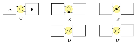
Figure 10. Two singular links ${\rm{S}}$ and ${\rm{S}}^{\prime}$ and links involved in their desingularization.

Take a link diagram ${\rm{C}}$ made by two disjoint knots diagrams ${\rm{A}}$ and ${\rm{B}}$ as shown in Figure 10. Then consider the singular links ${\rm{S}}$ and ${\rm{S}}^{\prime}$ in the same figure, obtained by modifying the link ${\rm{C}}$ only in the yellow disk. Evidently ${\rm{S}}$ and ${\rm{S}}^{\prime}$ are not isotopic, since ${\rm{S}}$ has two components, while ${\rm{S}}^{\prime}$ is a knot.

Theorem 15.

The singular links ${\rm{S}}$ and ${\rm{S}}^{\prime}$ are distinguished by $\Phi_{\mathsf{x},\mathsf{y}\,}$ if and only if $\mathsf{x}\not=\mathsf{y}\,$; however, they are distinguished by $\Psi_{\mathsf{x},\mathsf{x}}$.

Proof.

Notice that the link ${\rm{C}}$ corresponds to the cts–link $({\rm{C}},{{\bf 1}_{2}})$. We denote by $\tilde{\rm{C}}$ the link corresponding to the cts–link $({\rm{C}},\{\{1,2\}\})$. Since these links are not singular, we have $\Phi_{\mathsf{x},\mathsf{y}\,}({\rm{C}})=\Psi_{\mathsf{x},\mathsf{y}\,}({\rm{C}})$ and $\Phi_{\mathsf{x},\mathsf{y}\,}(\tilde{\rm{C}})=\Psi_{\mathsf{x},\mathsf{y}\,}(\tilde{\rm{C}})$. In particular

$$\Phi_{\mathsf{x},\mathsf{y}\,}({\rm{C}})=\Phi_{\mathsf{x},\mathsf{y}\,}({\rm{A}})\Phi_{\mathsf{x},\mathsf{y}\,}({\rm{B}})/(\mathsf{a}\,\sqrt{\mathsf{c}\,})\quad\text{and}\quad\Phi_{\mathsf{x},\mathsf{y}\,}(\tilde{\rm{C}})=\Phi_{\mathsf{x},\mathsf{y}\,}({\rm{A}})\Phi_{\mathsf{x},\mathsf{y}\,}({\rm{B}})\mathsf{f}\,/\sqrt{\mathsf{c}\,},$$

where $\mathsf{f}\,:=(\mathsf{u}\,\mathsf{c}\,-1)/(1-\mathsf{u}\,)=\mathsf{b}\,/\mathsf{a}\,$, see [2]. Observe that the knots ${\rm{D}}$ and ${\rm{D}}^{\prime}$ in Figure 10 are isotopic, both corresponding to the connected sum of the knots ${\rm{A}}$ and ${\rm{B}}$, so that $\Phi_{\mathsf{x},\mathsf{y}\,}({\rm{D}})=\Phi_{\mathsf{x},\mathsf{y}\,}({\rm{D}}^{\prime})=\Phi_{\mathsf{x},\mathsf{y}\,}({\rm{A}})\Phi_{\mathsf{x},\mathsf{y}\,}({\rm{B}})$. Using now the desingularization rule IV we get

$$\Phi_{\mathsf{x},\mathsf{y}\,}({\rm{S}})=\mathsf{x}\ \Phi_{\mathsf{x},\mathsf{y}\,}({\rm{D}})+\mathsf{y}\,\Phi_{\mathsf{x},\mathsf{y}\,}(\tilde{\rm{C}}),$$

$$\Phi_{\mathsf{x},\mathsf{y}\,}({\rm{S}}^{\prime})=\mathsf{x}\ \Phi_{\mathsf{x},\mathsf{y}\,}(\tilde{\rm{C}})+\mathsf{y}\,\Phi_{\mathsf{x},\mathsf{y}\,}({\rm{D}}^{\prime}).$$

Therefore,

$$\Phi_{\mathsf{x},\mathsf{y}\,}({\rm{S}})=\Phi({\rm{A}})\Phi_{\mathsf{x},\mathsf{y}\,}({\rm{B}})(\mathsf{x}+\mathsf{y}\,\mathsf{f}\,/\sqrt{\mathsf{c}\,}),$$

$$\Phi_{\mathsf{x},\mathsf{y}\,}({\rm{S}}^{\prime})=\Phi({\rm{A}})\Phi_{\mathsf{x},\mathsf{y}\,}({\rm{B}})(\mathsf{x}\ \mathsf{f}\,/\sqrt{\mathsf{c}\,}+\mathsf{y}\,).$$

These values coincide if and only if $\mathsf{x}=\mathsf{y}\,$. In fact, $\Phi_{\mathsf{x},\mathsf{y}\,}({\rm{S}})=\Phi_{\mathsf{x},\mathsf{y}\,}({\rm{S}}^{\prime})$ implies $(\mathsf{x}-\mathsf{y}\,)(1-\mathsf{f}\,/\sqrt{\mathsf{c}\,})=0$; now the equation $(1-\mathsf{f}\,/\sqrt{\mathsf{c}\,})=0$ has solutions $\mathsf{c}\,=1$ and $\mathsf{c}\,=\mathsf{u}\,^{-2}$, so $\Phi_{\mathsf{x},\mathsf{y}\,}$ distinguishes ${\rm{S}}$ and ${\rm{S}}^{\prime}$ if and only if $\mathsf{x}\not=\mathsf{y}\,$.

Consider now the polynomial $\Psi_{\mathsf{x},\mathsf{y}\,}$. Using the desingularization rule IV’, we get:

$$\Psi_{\mathsf{x},\mathsf{y}\,}({\rm{S}})=\mathsf{x}\ \Psi_{\mathsf{x},\mathsf{y}\,}({\rm{D}})+\mathsf{y}\,\Psi_{\mathsf{x},\mathsf{y}\,}({\rm{C}}),$$

$$\Psi_{\mathsf{x},\mathsf{y}\,}({\rm{S}}^{\prime})=\mathsf{x}\ \Psi_{\mathsf{x},\mathsf{y}\,}(\tilde{\rm{C}})+\mathsf{y}\,\Psi_{\mathsf{x},\mathsf{y}\,}({\rm{D}}^{\prime}).$$

Therefore,

$$\Psi_{\mathsf{x},\mathsf{y}\,}({\rm{S}})=\Psi_{\mathsf{x},\mathsf{y}\,}({\rm{A}})\Psi_{\mathsf{x},\mathsf{y}\,}({\rm{B}})(\mathsf{x}+\mathsf{y}\,/(\mathsf{a}\,\sqrt{\mathsf{c}\,})),$$

$$\Psi_{\mathsf{x},\mathsf{y}\,}({\rm{S}}^{\prime})=\Psi_{\mathsf{x},\mathsf{y}\,}({\rm{A}})\Psi_{\mathsf{x},\mathsf{y}\,}({\rm{B}})(\mathsf{x}\mathsf{f}\,/\sqrt{\mathsf{c}\,}+\mathsf{y}\,).$$

Now, if $\mathsf{x}=\mathsf{y}\,$, the equation $\Psi_{\mathsf{x},\mathsf{y}\,}({\rm{S}})=\Psi_{\mathsf{x},\mathsf{y}\,}({\rm{S}}^{\prime})$ implies $\mathsf{b}\,=1$, hence $\Psi_{\mathsf{x},\mathsf{x}}$ distinguishes ${\rm{S}}$ from ${\rm{S}}^{\prime}$. ∎

Remark 12.

Up to the present we don’t have examples showing that $\Psi_{\mathsf{x},\mathsf{y}\,}$ is able to distinguish pairs of classical singular links not distinguished $\Phi_{\mathsf{x},\mathsf{y}\,}$.

8.3. Comparison of our invariants with known invariants

Theorem 16.

Let ${\rm{L}}_{1}$ and ${\rm{L}}_{2}$ be two non isotopic links distinguished by $\mathcal{F}$ but not by $P$. Then any pair of singular links obtained by adding to ${\rm{L}}_{r}$ ($r=1,2$) a new component making a singular crossing and a negative crossing with whatever component of ${\rm{L}}_{r}$, is distinguished by $\Phi_{\mathsf{x},\mathsf{y}\,}$ and by $\Psi_{\mathsf{x},\mathsf{y}\,}$ but not by ${\rm{I}}_{PR}$.

Example 9.

The cts–links $({\rm{N}}_{1},{\bf 1}_{4})$ and $({\rm{N}}_{2},{\bf 1}_{4})$ in Figure 11 have one singularity. They are distinguished by the polynomials $\Phi_{\mathsf{x},\mathsf{y}\,}$, $\Psi_{\mathsf{x},\mathsf{y}\,}$, but not by $\Phi_{\mathsf{x},\mathsf{y}\,}^{\prime}$, $\Psi_{\mathsf{x},\mathsf{y}\,}^{\prime}$, nor by ${\rm{I}}_{PR}$. Indeed, by removing the orange component, we obtain the pair ${\rm{L}}11n356\{1,0\}$ and ${\rm{L}}11n434\{0,0\}$, distinguished by $\mathcal{F}$ but not by $\mathcal{F}^{\prime}$, nor by $P$, see [5].

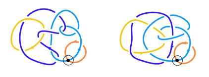
Figure 11. Two links $({\rm{N}}_{1},{\bf 1}_{4})$ and $({\rm{N}}_{2},{\bf 1}_{4})$ distinguished by the polynomials $\Phi_{\mathsf{x},\mathsf{y}\,}$, $\Psi_{\mathsf{x},\mathsf{y}\,}$, but not by $\Phi_{\mathsf{x},\mathsf{y}\,}^{\prime}$, $\Phi_{\mathsf{x},\mathsf{y}\,}^{\prime}$ , ${\rm{I}}_{PR}$ .

Theorem 17.

Let ${\rm{L}}_{1}$ and ${\rm{L}}_{2}$ be two non isotopic links distinguished by $\mathcal{F}^{\prime}$ but not by $P$. Then any pair of singular links obtained by adding to ${\rm{L}}_{r}$ ($r=1,2$) a new component making a singular crossing and a negative crossing with whatever component of ${\rm{L}}_{r}$, is distinguished by $\Phi_{\mathsf{x},\mathsf{y}\,}^{\prime}$ and by $\Psi_{\mathsf{x},\mathsf{y}\,}^{\prime}$ but not by ${\rm{I}}_{PR}$.

Example 10.

The cts–links $({\rm{M}}_{1},{\bf 1}_{4})$ and $({\rm{M}}_{2},{\bf 1}_{4})$ in Figure 12 have one singularity. They are distinguished by the polynomials $\Phi_{\mathsf{x},\mathsf{y}\,}$, $\Psi_{\mathsf{x},\mathsf{y}\,}$, $\Phi_{\mathsf{x},\mathsf{y}\,}^{\prime}$ and by $\Psi_{\mathsf{x},\mathsf{y}\,}^{\prime}$, but not ${\rm{I}}_{PR}$. Indeed, by removing the orange component, we obtain the pair ${\rm{L}}10n79\{1,1\}$ and ${\rm{L}}10n95\{1,0\}$, distinguished by $\mathcal{F}$ and by $\mathcal{F}^{\prime}$ but not by $P$, see respectively [5] and [9].

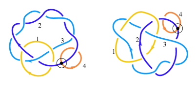
Figure 12. Two links $({\rm{M}}_{1},{\bf 1}_{4})$ and $({\rm{M}}_{2},{\bf 1}_{4})$ distinguished by the polynomials $\Phi_{\mathsf{x},\mathsf{y}\,}$, $\Psi_{\mathsf{x},\mathsf{y}\,}$, $\Phi_{\mathsf{x},\mathsf{y}\,}^{\prime}$, and $\Phi_{\mathsf{x},\mathsf{y}\,}^{\prime}$ but not by ${\rm{I}}_{PR}$ .

Proof of Theorem 16.

We use Example 10 to illustrate the proof. By the desingularization skein rule IV, we get for the pair $({\rm{M}}_{r},{\bf 1}_{4})$, $r=1,2$ (see the pairs A and C in Figure 13):

$$\Phi_{\mathsf{x},\mathsf{y}\,}({\rm{M}}_{r,\times}^{2,4},{\bf 1}_{4})=\mathsf{x}\ \Phi_{\mathsf{x},\mathsf{y}\,}({\rm{M}}_{r,0}^{2,2},\{\{1\}_{1},\{2\}_{2},\{3\}_{3}\})+\mathsf{y}\,\ \Phi_{\mathsf{x},\mathsf{y}\,}({\rm{M}}_{r,+}^{2,2},\{\{1\}_{1},\{2,4\}_{2},\{3\}_{3}\}).$$

Now, observe that the pair $({\rm{M}}_{r,+}^{2,2},\{\{1\}_{1},\{2,4\}_{2},\{3\}_{3}\})_{r=1,2}$ corresponds to the pair (A in Figure 13) of tied links $({\rm{L}}_{1}\tilde{\sqcup}O,L_{2}\tilde{\sqcup}O)$, where the symbol $\tilde{\sqcup}$ means that there is a tie between ${\rm{L}}$ and the unknot, while the pair $({\rm{M}}_{r,0}^{2,2},\{\{1\}_{1},\{2\}_{2},\{3\}_{3}\})_{r=1,2}$ (C in Figure 13) is the pair $({\rm{L}}_{1},{\rm{L}}_{2})$. Notice that, by Proposition 9, the value of $\Phi_{\mathsf{x},\mathsf{y}\,}$ on these pairs is the value of $\mathcal{F}$, which distinguishes the pair $({\rm{L}}_{1},{\rm{L}}_{2})$. Observe, moreover, that the value of $\mathcal{F}$ on ${\rm{L}}_{r}\tilde{\sqcup}O$ is the value of $\mathcal{F}$ on ${\rm{L}}_{r}$ by a coefficient independent from ${\rm{L}}_{r}$; therefore $\mathcal{F}$ distinguishes both pairs. As for $\Psi$, we have

$$\Psi_{\mathsf{x},\mathsf{y}\,}({\rm{M}}_{r,\times}^{2,4},{\bf 1}_{4})=\mathsf{x}\ \Psi_{\mathsf{x},\mathsf{y}\,}({\rm{M}}_{r,0}^{2,2},\{\{1\}_{1},\{2\}_{2},\{3\}_{3}\})+\mathsf{y}\,\ \Psi_{\mathsf{x},\mathsf{y}\,}({\rm{M}}_{r,+}^{2,4},{\bf 1}_{4}).$$

In Figure 13, the pair $({\rm{M}}_{r,+}^{2,4},{\bf 1}_{4})_{r=1,2}$ is the pair B and $({\rm{M}}_{r,0}^{2,2},\{\{1\}_{1},\{2\}_{2},\{3\}_{3}\})_{r=1,2}$ is again the pair C, i.e. $({\rm{L}}_{1},{\rm{L}}_{2})$. Also in this case, by Proposition 9, the value of $\Psi$ on these pairs is the value of $\mathcal{F}$, which distinguishes both pairs. ∎

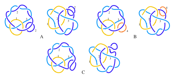
Figure 13. The links obtained by the desingularization rules of the pair $({\rm{M}}_{1},{\bf 1}_{4})$ and $({\rm{M}}_{2},{\bf 1}_{4})$.

Proof of Theorem 17.

For the values of $\Phi_{\mathsf{x},\mathsf{y}\,}^{\prime}$ and $\Psi_{\mathsf{x},\mathsf{y}\,}^{\prime}$, the argument is exactly the same by using $\mathcal{F}^{\prime}$ instead of $\mathcal{F}$. The value of ${\rm{I}}_{PR}$, instead, is obtained by substituting the partitions in the last formula by the partitions with a sole part, see Proposition 9. Thus the values of $\mathcal{F}$ and $\mathcal{F}^{\prime}$ coincide, again by Proposition 9, with the values of $P$, which does not distinguish such pairs. ∎

Proposition 11.

The pairs of singular links, denoted ${\rm{C}}_{1}$ and ${\rm{C}}_{2}$ in Figure 14, are both distinguished by $\Phi_{\mathsf{x},\mathsf{y}\,}$, $\Psi_{\mathsf{x},\mathsf{y}\,}$, $\Phi_{\mathsf{x},\mathsf{y}\,}^{\prime}$ and by $\Psi_{\mathsf{x},\mathsf{y}\,}^{\prime}$, but are not distinguished by ${\rm{I}}_{PR}$.

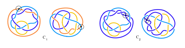
Figure 14. Pairs of links distinguished by the polynomials $\Phi_{\mathsf{x},\mathsf{y}\,}$ and $\Psi_{\mathsf{x},\mathsf{y}\,}$.

Proof.

Let us denote by $({\rm{L}}_{1},{\rm{L}}_{2})$ the pair of classical links ${\rm{L}}10n79\{1,1\}$ and ${\rm{L}}10n95\{1,0\}$, and by $({\rm{L}}_{3},{\rm{L}}_{4})$ the pair of classical links ${\rm{L}}11n325\{1,1\}$ and ${\rm{L}}11n424\{0,0\}$, see Figure 15. All these links have 3 components, and both pairs are distinguished by the polynomials $\mathcal{F}$ and $\mathcal{F}^{\prime}$ but not by the $P$.

Consider now the pair of classical links $({\rm{M}}_{1},{\rm{M}}_{2})$ in Figure 15, with four components. Also this pair is not distinguished by $P$ but is distinguished by $\mathcal{F}$ and by $\mathcal{F}^{\prime}$, also when two of the four components belong to the same part.

For the pair ${\rm{C}}_{1}$ of singular links ${\rm{S}}_{1}$ and ${\rm{S}}_{2}$ we apply the desingularization rule IV and we obtain:

$$\Phi_{\mathsf{x},\mathsf{y}\,}({\rm{S}}_{1})=\mathsf{x}\ \Phi_{\mathsf{x},\mathsf{y}\,}({\rm{L}}_{1},{\bf 1}_{3})+\mathsf{y}\,\Phi_{\mathsf{x},\mathsf{y}\,}({\rm{M}}_{1}^{3,4},\{\{3,4\}\}),$$

$$\Phi_{\mathsf{x},\mathsf{y}\,}({\rm{S}}_{2})=\mathsf{x}\ \Phi_{\mathsf{x},\mathsf{y}\,}({\rm{L}}_{2},{\bf 1}_{3})+\mathsf{y}\,\Phi_{\mathsf{x},\mathsf{y}\,}({\rm{M}}_{2}^{3,4},\{\{3,4\}\}).$$

For the pair ${\rm{C}}_{2}$ of singular links ${\rm{S}}_{3}$ and ${\rm{S}}_{4}$ we apply the desingularization rule IV and we obtain:

$$\Phi_{\mathsf{x},\mathsf{y}\,}({\rm{S}}_{3})=\mathsf{x}\ \Phi_{\mathsf{x},\mathsf{y}\,}({\rm{M}}_{1}^{2,4},\{\{2,4\}\})+\mathsf{y}\,\Phi_{\mathsf{x},\mathsf{y}\,}({\rm{L}}_{3},{\bf 1}_{3}),$$

$$\Phi_{\mathsf{x},\mathsf{y}\,}({\rm{S}}_{4})=\mathsf{x}\ \Phi_{\mathsf{x},\mathsf{y}\,}({\rm{M}}_{2}^{2,4},\{\{2,4\}\})+\mathsf{y}\,\Phi_{\mathsf{x},\mathsf{y}\,}({\rm{L}}_{4},1_{3}).$$

Now, by Proposition 9, we have that $\Phi_{\mathsf{x},\mathsf{y}\,}({\rm{L}}_{r},{\bf 1}_{3})=\mathcal{F}({\rm{L}}_{r})$ and the value of $\Phi_{\mathsf{x},\mathsf{y}\,}$ on $({\rm{M}}_{r}^{2,4},\{\{2,4\}\})$ and $({\rm{M}}_{r}^{2,4},\{\{3,4\}\})$ coincides with that of $\mathcal{F}$.

Figure 15. Two pairs of singular links distinguished by the polynomials $\Phi_{\mathsf{x},\mathsf{y}\,}$, $\Psi_{\mathsf{x},\mathsf{y}\,}$ but not by ${\rm{I}}_{PR}$.

We do not write the desingularization rules for $\Phi_{\mathsf{x},\mathsf{y}\,}^{\prime}$, since they give the same expressions by replacing $\Phi_{\mathsf{x},\mathsf{y}\,}$ with $\Phi_{\mathsf{x},\mathsf{y}\,}^{\prime}$ and $\mathcal{F}$ with $\mathcal{F}^{\prime}$. So, $\Phi_{\mathsf{x},\mathsf{y}\,}$ and $\Phi_{\mathsf{x},\mathsf{y}\,}^{\prime}$ distinguish the pairs ${\rm{C}}_{1}$ and ${\rm{C}}_{2}$ as a consequence of the fact that $\mathcal{F}$ and $\mathcal{F}^{\prime}$ distinguish the links obtained by the desingularization. The fact that ${\rm{I}}_{PR}$ does not distinguish these pairs, follows from the fact that $P$ does not distinguish the corresponding pairs, see Proposition 9 items (2) and (5).

For the polynomial $\Psi_{\mathsf{x},\mathsf{y}\,}$, the desingularization rule applied to the pair ${\rm{C}}_{1}$ of singular links ${\rm{S}}_{1}$ and ${\rm{S}}_{2}$ gives:

$$\Psi_{\mathsf{x},\mathsf{y}\,}({\rm{S}}_{1})=\mathsf{x}\ \mathcal{F}({\rm{L}}_{1})+\mathsf{y}\,\mathcal{F}({\rm{M}}_{1},{\bf 1}_{4}),$$

$$\Psi_{\mathsf{x},\mathsf{y}\,}({\rm{S}}_{2})=\mathsf{x}\ \mathcal{F}({\rm{L}}_{2})+\mathsf{y}\,\mathcal{F}({\rm{M}}_{2},{\bf 1}_{4}).$$

The same holds for $\Psi^{\prime}$, replacing $\mathcal{F}$ with $\mathcal{F}^{\prime}$. Now, since the singularities of ${\rm{S}}_{3}$ and ${\rm{S}}_{4}$ involve a unique component, the desingularization rules for $\Psi$ and $\Psi^{\prime}$ coincide with those for $\Phi_{\mathsf{x},\mathsf{y}\,}$. Thus, the proof follows as that for $\Phi_{\mathsf{x},\mathsf{y}\,}$.

∎

Finally, in the proposition below we show the behavior of our invariants and of ${\rm I}_{PR}$ on a pair of links with two singularities.

Proposition 12.

The pair ${\rm{C}}_{3}$ of singular links in Figure 16 with two singularities is distinguished by $\Phi_{\mathsf{x},\mathsf{y}\,}$, $\Psi_{\mathsf{x},\mathsf{y}\,}$, $\Phi_{\mathsf{x},\mathsf{y}\,}^{\prime}$, $\Psi_{\mathsf{x},\mathsf{y}\,}^{\prime}$ and by ${\rm{I}}_{PR}$.

Proof.

The desingularizations of the two singular links give four pairs of classical links, some of them already considered in Proposition 11. However, the presence of other pairs, distinguished by the classical polynomials, makes the original singular pair distinguished also by ${\rm{I}}_{PR}$. ∎

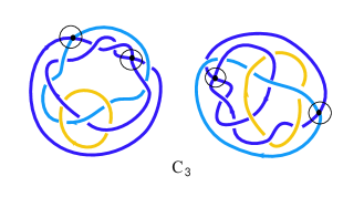
Figure 16. Two singular links distinguished by the polynomials $\Phi_{\mathsf{x},\mathsf{y}\,}$, $\Phi^{\prime}_{\mathsf{x},\mathsf{y}\,}$, $\Psi_{\mathsf{x},\mathsf{y}\,}$, $\Psi^{\prime}_{\mathsf{x},\mathsf{y}\,}$ and ${\rm{I}}_{PR}$.

References

- [1] F. Aicardi, J. Juyumaya, An algebra involving braids and ties, ICTP Preprint IC/2000/179. See https://arxiv.org/pdf/1709.03740.pdf.
- [2] F. Aicardi and J. Juyumaya, Tied Links, J. Knot Theory Ramifications, 25 (2016), no. 9, 1641001, 28 pp.
- [3] F. Aicardi and J. Juyumaya, Markov trace on the algebra of braid and ties, Moscow Math. J. 16 (2016), no. 3, 397–431.
- [4] F. Aicardi and J. Juyumaya, Kauffman type invariants for tied links, Math. Z. (2018) 289:567–591.
- [5] F. Aicardi, New invariants of links from a skein invariant of colored links, arXiv:1512.00686.
- [6] J.C. Baez, Link invariants of finite type and perturbation theory, Lett. Math. Phys. 26 (1992), no. 1, 43–51.
- [7] J.S. Birman, New points of view in knot theory, Bull. Amer. Math. Soc. (N.S.) 28 (1993), no. 2, 253–287.
- [8] J.C. Cha, C. Livingston, LinkInfo: Table of Knot Invariants, http://www.indiana.edu/linkinfo, April 16, 2015.
- [9] M. Chlouveraki et al., Identifying the Invariants for Classical Knots and Links from the Yokonuma–Hecke Algebras, Int. Math. Res. Not. IMRN 2020, no. 1, 214–286.
- [10] J. Espinoza and S. Ryom–Hansen, Cell structures for the Yokonuma–Hecke algebra and the algebra of braids and ties, J. Pure Appl. Algebra 222 (2018), no. 11, 3675–3720.
- [11] B. Gemein, Singular braids and Markov’s theorem, J. Knot Theory Ramifications 6 (1997), no. 4, 441–454.
- [12] N. Jacon and L. Poulain d’Andecy, Clifford theory for Yokonuma–Hecke algebras and deformation of complex reflection groups, J. London Math. Soc. (2) 96 (2017) 501–523.
- [13] V.F.R. Jones, Hecke algebra representations of braid groups and link polynomials, Ann. Math. 126 (1987), 335–388.
- [14] J. Juyumaya and S. Lambropoulou, An invariant for singular knots, J. Knot Theory Ramifications 18 (2009), no. 6, 825–840.
- [15] L.H. Kauffman and P. Vogel, Link polynomials and a graphical calculus, J. Knot Theory Ramifications 1 (1992), no. 1, 59–104.
- [16] T. Mansour, Combinatorics of set partitions, Discrete Mathematics and its Applications (Boca Raton). CRC Press, Boca Raton, FL, 2013. xxviii+587 pp. ISBN: 978-1-4398-6333-6.
- [17] I. Marin, Artin Groups and Yokonuma–Hecke Algebras, International Mathematics Research Notices, 2018 (2018), no. 13, 4022–4062.
- [18] L. Paris and L. Rabenda, Singular Hecke algebras, Markov traces and HOMFLY–type invariants, Annales de l’Institut Fourier 58, no. 7 (2008), 2414–2443.
- [19] S. Ryom–Hansen, On the Representation Theory of an Algebra of Braids and Ties, J. Algebr. Comb. 33 (2011), 57–79.
- [20] L. Smolin, Knot theory, loop space and the diffeomorphism group, New perspectives in canonical gravity, 245–266, Monogr. Textbooks Phys. Sci. Lecture Notes, 5, Bibliopolis, Naples, 1988.