Origin of the hemispheric asymmetry of solar activity

The frequency spectrum of the hemispheric asymmetry of solar activity shows enhanced power for the period ranges around 8.5 years and between 30 and 50 years. This can be understood as the sum and beat periods of the superposition of two dynamo modes: a dipolar mode with a (magnetic) period of about 22 years and a quadrupolar mode with a period between 13 and 15 years. An updated Babcock-Leighton-type dynamo model with weak driving as indicated by stellar observations shows an excited dipole mode and a damped quadrupole mode in the correct range of periods. Random excitation of the quadrupole by stochastic fluctuations of the source term for the poloidal field leads to a time evolution of activity and asymmetry that is consistent with the observational results.

1 Introduction

The various manifestations of solar magnetic activity, such as sunspots, prominences, and flares, typically are distributed unevenly between the northern and southern hemisphere of the Sun (cf. Norton et al., 2014; Hathaway, 2015; Deng et al., 2016, and references therein). Normally, this hemispheric asymmetry does not exceed a level of about 20% (Norton & Gallagher, 2010). However, during the Maunder minimum in the second half of the 17th century nearly all of the few sunspots observed during this time appeared in the southern hemisphere (Ribes & Nesme-Ribes, 1993; Vaquero et al., 2015). Various studies demonstrated that the asymmetry has systematic components that cannot be explained by random fluctuations of flux emergence alone (e.g. Carbonell et al., 1993, 2007; Deng et al., 2016). It has been suggested that there is also a systematic variation of the phase shift of the activity cycle between the hemispheres (e.g. Zolotova et al., 2010; Norton & Gallagher, 2010; Muraközy & Ludmány, 2012; McIntosh et al., 2013).

A number of studies investigate the hemispheric asymmetry by way of frequency analysis (e.g. Deng et al., 2016, and references therein). Ballester et al. (2005) demonstrated that the commonly used normalised asymmetry parameter, $(N-S)/(N+S)$, where $N$ and $S$ represent the quantity under consideration in the northern and southern hemisphere, respectively, is not a sensible choice for this kind of analysis: the denominator introduces a contamination of the power spectrum by the strong 11-year periodicity. Ballester et al. (2005) instead carry out a frequency analysis of the un-normalised asymmetry, $A_{\rm N}-A_{\rm S}$, of the monthly hemispheric sunspot areas between 1874 and 2004. They use the dataset compiled by D. Hathaway, based upon the Greenwich Photoheliographic Results and the USAF/SOON data, and find three significant periods with false-alarm probabilities below 0.5%: 43.25, 8.65, and 1.44 years. Very similar periods (among others) are also found by Knaack et al. (2004), who use the same dataset, while Deng et al. (2016) reported periods of 51.3 and 8.7 years. Studying the hemispheric asymmetry of filaments between 1919 and 1989, Duchlev & Dermendjiev (1996) find periods of 35 and 8.75 years, although they considered only the former to be statistically significant. On the other hand, Chang (2009) suggests that only the period around nine years in the asymmetry of sunspot areas is significant while other periodicities may not. Since the length of the various data series does not exceed about 150 years, the frequency resolution for the longer periods is rather low. Thus we may conclude from these studies that there is evidence for a short period (around 9 years) and a long period (between 35 and 50 years) in the data for the un-normalised asymmetry, while the 11-year cycle does not significantly appear.

In this paper, we show that the periods found in the observational data for the absolute hemispheric asymmetry occur naturally as the beat period and the sum period of a mixed-mode dynamo solution comprised of a dipole mode with a (magnetic) period of about 22 years and a quadrupole mode with a period between 13 and 15 years. We also find that periods in this range are reproduced by the updated Babcock-Leighton dynamo model of Cameron & Schüssler (2017a) in the case of weak dynamo driving as suggested by stellar observations. While the dipole mode is permanently excited, the quadrupole is subcritical and only occasionally kicks in through random fluctuations of the poloidal source term.

This paper is structured as follows. In Sect. 2, we present a simple model of superposed harmonic oscillations to illustrate the origin of the various periodicities. From the observed periods of the hemispheric asymmetry, we determine the periods of the antisymmetric (dipole) mode and the symmetric (quadrupole) mode. Sect. 3 gives the corresponding results obtained with the updated Babcock-Leighton model. We summarise our conclusions in Sect. 4.

2 Hemispheric aymmetry by superposition of symmetric and antisymmetric modes

As a simple illustration of the possible origin of the various periods detected in the sunspot area data (full disk, hemispheric, and asymmetry), we have considered the superposition of two harmonic oscillations with different frequencies. They are taken to represent two dynamo modes for the toroidal field, $B_{\phi}$: one mode is antisymmetric with respect to the equator (dipole parity, frequency $\omega_{D}$), the other mode is symmetric (quadrupole parity, frequency $\omega_{Q}$). Since we are only interested in the frequencies resulting from the superposition, we set the amplitudes of the modes to be equal and normalise them to unity. Taking the activity index to be proportional to $B^{2}_{\phi}$, that is, the square of the superposed modes, we have for the indices in the northern hemisphere, $A_{\rm N}$, and in the southern hemisphere, $A_{\rm S}$, respectively:

$$A_{\rm N} = \left[\sin(\omega_{D}t)+\sin(\omega_{Q}t)\right]^{2},\;{\rm and}$$

$$A_{\rm S} = \left[-\sin(\omega_{D}t)+\sin(\omega_{Q}t)\right]^{2}.$$ (1)

The indices for the full disk and for the (absolute) asymmetry are then given by the sum and the difference, respectively, of the hemispheric signals, viz.

$$A_{\rm N}+A_{\rm S} = 2\sin^{2}(\omega_{D}t)+2\sin^{2}(\omega_{Q}t)$$

$$A_{\rm N}-A_{\rm S} = 4\sin(\omega_{D}t)\sin(\omega_{Q}t)$$ (2)

$$= 2\cos[(\omega_{Q}-\omega_{D})t]-2\cos[(\omega_{Q}+\omega_{D})t]\,,$$

where $\omega_{Q}-\omega_{D}\equiv\omega_{b}$ is the beat frequency and $\omega_{Q}+\omega_{D}\equiv\omega_{s}$ is the sum frequency. It is clear from Eqs. (1) and (2) that the frequencies appearing in the various quantities are different: while only the double frequencies, $2\omega_{D}$ and $2\omega_{Q}$, show up in the full-disk index, the absolute asymmetry is governed solely by the beat and the sum frequencies. The hemispheric indices are affected by all four of these frequencies. In terms of periods, we have

$$P_{b}=\frac{P_{D}P_{Q}}{P_{D}-P_{Q}}$$ (3)

for the beat period and

$$P_{s}=\frac{P_{D}P_{Q}}{P_{D}+P_{Q}}$$ (4)

for the period corresponding to the sum frequency, where $P_{D}=2\pi/\omega_{D}$ and $P_{Q}=2\pi/\omega_{Q}$, respectively, are the periods of the dipole and quadrupole dynamo modes.

Consistent with the expectation from this simple model, the analysis of the absolute asymmetry of hemispheric sunspot areas by Ballester et al. (2005) results in two dominant periods, $43.25\,$years and $8.65\,$years, while the 11-year cycle period (dominated by the dipole) does not appear. Tentatively identifying these two observed periods with the beat and sum periods, we can use Eqs. (3) and (4) determine the dipole period, $P_{D}$, and the quadrupole period, $P_{Q}$. With $P_{b}=43.25\,$years and $P_{s}=8.65\,$years we obtain $P_{D}=21.6\,$years and $P_{Q}=14.4\,$years. If we take into account the limited frequency resolution and assume a range between 30 years and 50 years for the for the longer (beat) period, we find $P_{D}\approx 21...24\,$years and $P_{Q}\approx 13...15\,$years. The obtained dipole period is consistent with the 11-year activity cycle. This suggests that our simple model is a viable representation of the asymmetry data, suggesting the presence of a solar quadrupole dynamo mode with a period between 13 and $15\,$years. Incidentally, Muñoz-Jaramillo et al. (2013) show that considering both the dipole and quadrupole moments of the poloidal field during cycle minima improves the predictive power for the amplitude of the subsequent cycle (see also Goel & Choudhuri, 2009).

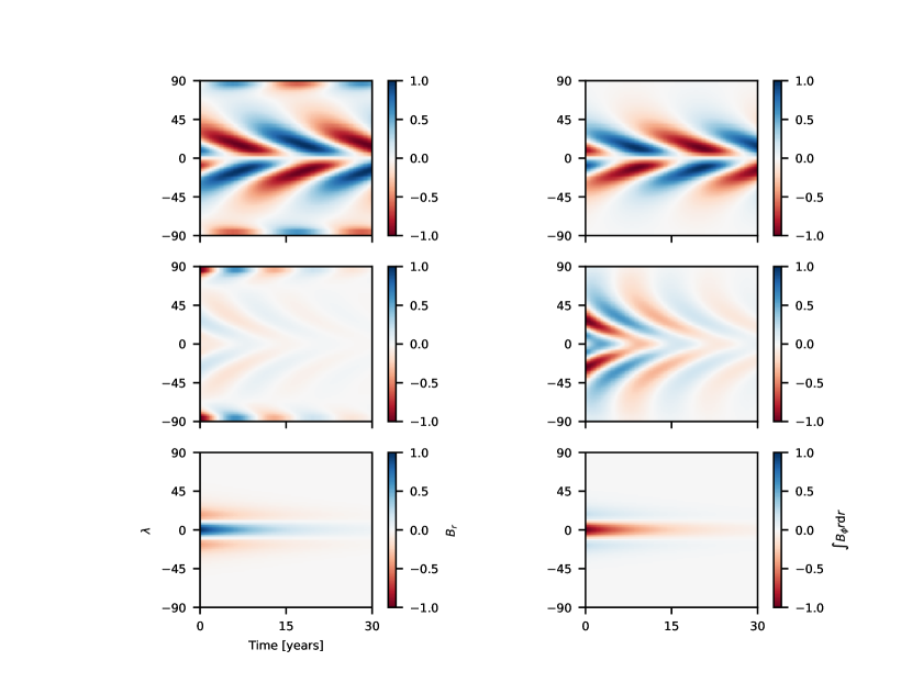
Figure 1: Spatio-temporal structure of the first linear eigenmodes obtained with the updated Babcock-Leighton model (Cameron & Schüssler, 2017a). Shown are latitude-time diagrams of the azimuthally averaged radial surface field (left panels) and the radially integrated toroidal flux (right panels). The three modes shown are an excited oscillatory dipolar mode (top panels), a damped oscillatory quadrupolar mode (middle panels) and a damped stationary quadrupolar mode (bottom panels). The quantities are normalised to their individual maxima in all cases.

3 Dynamo model

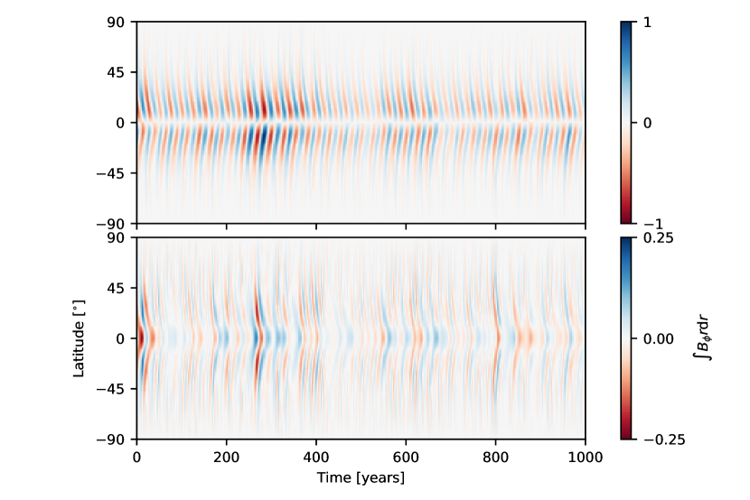
Figure 2: Non-linear case with random fluctuations of the poloidal source term. Shown are time-latitude diagrams of the antisymmetric (dipolar, upper panel) and symmetric (quadrupolar, lower panel) components of the radially integrated toroidal magnetic flux. The linearly damped oscillatory and stationary quadrupolar modes are occasionally excited.

Hemispheric asymmetry in dynamo models has been studied by various authors (reviewed by Norton et al., 2014; Brun et al., 2015). There are two main approaches that have been followed: non-linear effects and stochastic fluctuations. Non-linearity in the dynamo equations can lead to the coupling of symmetric (even) and antisymmetric (odd) modes, strong hemispheric asymmetry, and the occurence of extended ‘grand minima’ (e.g. Kleeorin & Ruzmaikin, 1984; Tobias, 1997; Brooke et al., 1998; Hotta & Yokoyama, 2010; Weiss & Tobias, 2016). Alternatively, stochastic fluctuations of model ingredients (such as mean-field $\alpha$-effect or meridional flow speed) can also lead to hemispheric asymmetry as well as to the (temporal) excitation of higher eigenmodes and mixed-mode solutions (e.g. Hoyng et al., 1994; Olemskoy & Kitchatinov, 2013; Belucz & Dikpati, 2013; Passos et al., 2014). Combinations of both effects have been studied as well (e.g. Moss et al., 1992; Schmitt et al., 1996; Mininni & Gómez, 2002; Charbonneau, 2007; Moss & Sokoloff, 2017). For example, Sokoloff et al. (2010) and Usoskin et al. (2009) find that random fluctuations of the dynamo excitation in a simple Parker-type dynamo wave model can lead to substantial mixing between dipole and quadrupole modes, particularly so during episodes of low dynamo amplitude akin to grand minima of solar activity. Global 3D-MHD simulations exhibit features that are similar to the results provided by the more idealised approaches (Norton et al., 2014; Brun et al., 2015; Käpylä et al., 2016).

Dominance of the dipole mode and relatively weak hemispheric asymmetry can be provided by sufficiently strong hemispheric coupling via turbulent diffusion, cross-equator flows, or cross-equator cancellation of toroidal flux (Norton et al., 2014; Cameron & Schüssler, 2016). Moreover, observational gyrochronology of solar-like stars (van Saders et al., 2016; Metcalfe et al., 2016) indicates weak excitation of the solar dynamo. In this case, there is the possibility that only the lowest (dipole) dynamo mode is excited while the quadrupole mode is linearly damped.

As an illustration for the stochastic excitation of a mixed-mode dynamo solution that is consistent with the observed features of the hemispheric asymmetry, we show results from the updated Babcock-Leighton model of Cameron & Schüssler (2017a) with stochastic fluctuations of the poloidal field source (see Sect. 3 in Cameron & Schüssler, 2017b). The parameters for this case were chosen according to the following observational constraints: (a) excited dipole mode with a period of about 22 years, (b) phase difference between polar radial field and subsurface toroidal flux of about $90^{\circ}$, (c) no linearly excited quadrupolar mode. In such a case, linearly damped quadrupole modes can be stochastically excited by the fluctuations of the poloidal field source, so that a mixed-mode solution occasionally develops. The parameters for the case discussed here were: $\eta_{R_{\odot}}=150$ km${}^{2}\cdot$s^-1 and $\eta_{0}=50$ km${}^{2}\cdot$s^-1 for the turbulent magnetic diffusivities in the near-surface layers and in the bulk of the convection zone, respectively; $\alpha_{0}=1.3$ m$\cdot$s^-1 for the average poloidal source level, and $\sigma^{*}=0.046$ for the fluctuation level. The source fluctuations are local in latitude (in steps of 1 degree) and in time (in steps of 1 day), governed by a Wiener process with a variance of 1 radian^-1 after 11 years. This corresponds to a RMS fluctuation of the source term of about 5% (integrated over 11 years and one radian). We used the near-surface meridional flow as determined by Hathaway & Rightmire (2011) and $V_{0}=1.7$ m$\cdot$s^-1 for the amplitude of the equatorward meridional return flow affecting the toroidal flux in the convection zone. The critical integrated flux for the cut-off non-linearity in the poloidal source term was $10^{24}\,$Mx.

Linear analysis shows that for these parameters we have an excited oscillating antisymmetric (dipolar) mode with a period of 22.4 years ($\alpha/\alpha_{\rm crit}=1.06$) and a damped symmetric (quadrupolar) mode with a period of 13.5 years and a damping time of 13 years ($\alpha/\alpha_{\rm crit}=0.12$). In addition, there is a symmetric stationary mode with a damping time of about 10 years. Fig. 1 shows the spatio-temporal structure of these linear modes. Fig. 2 shows the symmetric and antisymmetric components of a simulation of the non-linear case with fluctuations. The quadrupolar (symmetric) modes are occasionally excited owing to the random fluctuations of the poloidal source term. In addition, there are variations of the dynamo amplitude. The ratio of the RMS values of the toroidal field variable between the quadrupole and the dipole modes is about 0.18. Owing to the non-linearity, the oscillation periods become somewhat variable and their mean values differ from their linear counterparts: 20.8 years for the dipole and 14.7 years for the oscillatory quadrupole. According to Eqs. (3) and (4), the linear periods lead to a beat period $P_{b}=34\,$years and a sum period $P_{s}=8.4\,$years while the non-linear periods give $P_{b}=50.1\,$years and $P_{s}=8.6\,$years. Hence, the beat period is much more sensitive to period variations than the sum period. We therefore expect periodic signals in the absolute asymmetry (for instance of the toroidal flux taken as an activity indicator) around 8.5 years ($P_{s}$) and in the range 30-50 years ($P_{b}$). Such signals can in fact be seen in Fig. 3, which shows power spectra of the absolute hemispheric asymmetry of the hemispheric toroidal flux integrated between $0^{\circ}$ and $\pm 40^{\circ}$ latitude (red curve) from the Babcock-Leighton model in comparison with that of the observed sunspot area (blue curve). This is consistent with the expectation from the simple model described in Sec. 2. The widths of the peaks results from the variability of the (non-linear) periods, the damping of the quadrupole mode, as well as from realisation noise. The dynamo model serves only as an illustration of the proposed mechanism behind the hemispheric asymmetry; we have made no attempt to fine-tune the parameters in order to have a precise agreement of the model result with the observed peak at 43 years. It suffices to state that the updated Babcock-Leighton model with low excitation and stochastic fluctuations of the poloidal source yields results that are consistent with the observed features.

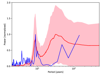
Figure 3: Power spectra of the absolute hemispheric asymmetry. The blue curve corresponds to the absolute asymmetry of the sunspot areas from the Greenwich/SOON data. The red curve gives the average power spectrum for the difference of the unsigned toroidal fluxes integrated between the equator and $\pm 30/40^{\circ}$ latitude). The latter is based on 1000 realizations of 500 year each from the Babcock-Leighton model with source fluctuations (Cameron & Schüssler, 2017b). The pink shading indicates $\pm$1 standard deviation from the mean.

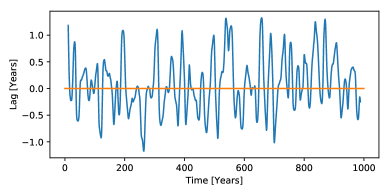
Figure 4: Phase lag (time shift) between the toroidal fluxes in the northern and southern hemispheres for a 1000-yr stretch of a simulation on the basis of the updated Babcock-Leighton model. The lag was determined by using the cross-covariance between segments with a length of 20 years.

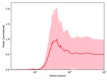
Figure 5: Average power spectrum of the time shift between the hemispheres from 20 realizations of the updated Babcock-Leighton dynamo of 10,000 year length each. The shading indicates $\pm 1$ standard deviations.

We may also consider the phase lag between the hemispheres. From the sunspot record, some authors suggest a periodicity of the phase lag of eight cycles, that is, about 90 years (e.g. Zolotova et al., 2010; Norton & Gallagher, 2010; Muraközy & Ludmány, 2012), or even twelve cycles (e.g. Zhang & Feng, 2015). Some caution seems to be in order in view of the fact that the time series used are not much longer than the inferred periods. Using a cross-correlation method, McIntosh et al. (2013) find long-term variations with the hemispheres alternating in phase shift for intervals between 30 and 60 years since 1874. On the other hand, on the basis of the simple model in Sec. 2, we expect a periodicity of the phase lag with the beat period, $P_{b}$. We have applied a method similar to that used by McIntosh et al. (2013) to the results from the updated Babcock-Leighton model, simulated with the same parameters as described above. Using the hemispheric toroidal flux integrated from the equator to $\pm 40^{\circ}$ latitude, we considered 20-year segments from 50 simulations covering 10,000 years each. Removing the mean of the signals and applying a Hann window to the segments, we then calculated the cross-covariance between the northern and southern hemisphere signals and determined the time lag between the hemispheres by considering the maximum of the cross-covariance. A typical example for the temporal variation of the lag is shown in Fig. 4. It suggest a modulation with a period around 30 years. This is confirmed by the power spectrum shown in Fig. 5. The curve gives the mean power spectrum for 1000 realizations of 500 years length each while the shading indicates $\pm 1$ standard deviation. Comparison with Fig. 3 shows that the main power appears in the range of the beat period of 30-50 years, but there is considerable power at longer periods as well, indicating longer-term modulations. This is also obvious from Fig. 4, where the sign of the lag often remains the same for intervals exceeding the beat period.

4 Conclusions

We have shown that the observed power spectrum of the absolute hemispheric asymmetry of solar activity can be naturally explained by the superposition of an excited dipolar mode (toroidal field antisymmetric with respect to the equator) with a magnetic period of about 22 years and a linearly damped, but randomly excited quadrupolar mode (toroidal field symmetric with respect to the equator) with a period between 13 and 15 years. The updated Babcock-Leighton dynamo model of Cameron & Schüssler (2017a) with weak excitation reproduces these conditions and yields a time evolution of the magnetic field and its asymmetry that is consistent with the observations.

References

- Ballester et al. (2005) Ballester, J. L., Oliver, R., & Carbonell, M. 2005, A&A, 431, L5
- Belucz & Dikpati (2013) Belucz, B. & Dikpati, M. 2013, ApJ, 779, 4
- Brooke et al. (1998) Brooke, J. M., Pelt, J., Tavakol, R., & Tworkowski, A. 1998, A&A, 332, 339
- Brun et al. (2015) Brun, A. S., Browning, M. K., Dikpati, M., Hotta, H., & Strugarek, A. 2015, Space Sci. Rev., 196, 101
- Cameron & Schüssler (2016) Cameron, R. H. & Schüssler, M. 2016, A&A, 591, A46
- Cameron & Schüssler (2017a) —. 2017a, A&A, 599, A52
- Cameron & Schüssler (2017b) —. 2017b, ApJ, 843, 111
- Carbonell et al. (1993) Carbonell, M., Oliver, R., & Ballester, J. L. 1993, A&A, 274, 497
- Carbonell et al. (2007) Carbonell, M., Terradas, J., Oliver, R., & Ballester, J. L. 2007, A&A, 476, 951
- Chang (2009) Chang, H.-Y. 2009, New A, 14, 133
- Charbonneau (2007) Charbonneau, P. 2007, Advances in Space Research, 40, 899
- Deng et al. (2016) Deng, L. H., Xiang, Y. Y., Qu, Z. N., & An, J. M. 2016, AJ, 151, 70
- Duchlev & Dermendjiev (1996) Duchlev, P. I. & Dermendjiev, V. N. 1996, Sol. Phys., 168, 205
- Goel & Choudhuri (2009) Goel, A. & Choudhuri, A. R. 2009, Research in Astronomy and Astrophysics, 9, 115
- Hathaway (2015) Hathaway, D. H. 2015, Living Reviews in Solar Physics, 12, 12, http://link.springer.com/article/10.1007/lrsp
- Hathaway & Rightmire (2011) Hathaway, D. H. & Rightmire, L. 2011, ApJ, 729, 80
- Hotta & Yokoyama (2010) Hotta, H. & Yokoyama, T. 2010, ApJ, 714, L308
- Hoyng et al. (1994) Hoyng, P., Schmitt, D., & Teuben, L. J. W. 1994, A&A, 289, 265
- Käpylä et al. (2016) Käpylä, M. J., Käpylä, P. J., Olspert, N., et al. 2016, A&A, 589, A56
- Kleeorin & Ruzmaikin (1984) Kleeorin, N. I. & Ruzmaikin, A. A. 1984, Astronomische Nachrichten, 305, 265
- Knaack et al. (2004) Knaack, R., Stenflo, J. O., & Berdyugina, S. V. 2004, A&A, 418, L17
- McIntosh et al. (2013) McIntosh, S. W., Leamon, R. J., Gurman, J. B., et al. 2013, ApJ, 765, 146
- Metcalfe et al. (2016) Metcalfe, T. S., Egeland, R., & van Saders, J. 2016, ApJ, 826, L2
- Mininni & Gómez (2002) Mininni, P. D. & Gómez, D. O. 2002, ApJ, 573, 454
- Moss et al. (1992) Moss, D., Brandenburg, A., Tavakol, R., & Tuominen, I. 1992, A&A, 265, 843
- Moss & Sokoloff (2017) Moss, D. L. & Sokoloff, D. D. 2017, Astronomy Reports, 61, 878
- Muñoz-Jaramillo et al. (2013) Muñoz-Jaramillo, A., Balmaceda, L. A., & DeLuca, E. E. 2013, Physical Review Letters, 111, 041106
- Muraközy & Ludmány (2012) Muraközy, J. & Ludmány, A. 2012, MNRAS, 419, 3624
- Norton et al. (2014) Norton, A. A., Charbonneau, P., & Passos, D. 2014, Space Sci. Rev., 186, 251
- Norton & Gallagher (2010) Norton, A. A. & Gallagher, J. C. 2010, Sol. Phys., 261, 193
- Olemskoy & Kitchatinov (2013) Olemskoy, S. V. & Kitchatinov, L. L. 2013, ApJ, 777, 71
- Passos et al. (2014) Passos, D., Nandy, D., Hazra, S., & Lopes, I. 2014, A&A, 563, A18
- Ribes & Nesme-Ribes (1993) Ribes, J. C. & Nesme-Ribes, E. 1993, A&A, 276, 549
- Schmitt et al. (1996) Schmitt, D., Schüssler, M., & Ferriz-Mas, A. 1996, A&A, 311, L1
- Sokoloff et al. (2010) Sokoloff, D., Arlt, R., Moss, D., Saar, S. H., & Usoskin, I. 2010, in IAU Symposium, Vol. 264, Solar and Stellar Variability: Impact on Earth and Planets, ed. A. G. Kosovichev, A. H. Andrei, & J.-P. Rozelot, 111–119
- Tobias (1997) Tobias, S. M. 1997, A&A, 322, 1007
- Usoskin et al. (2009) Usoskin, I. G., Sokoloff, D., & Moss, D. 2009, Sol. Phys., 254, 345
- van Saders et al. (2016) van Saders, J. L., Ceillier, T., Metcalfe, T. S., et al. 2016, Nature, 529, 181
- Vaquero et al. (2015) Vaquero, J. M., Nogales, J. M., & Sánchez-Bajo, F. 2015, Advances in Space Research, 55, 1546
- Weiss & Tobias (2016) Weiss, N. O. & Tobias, S. M. 2016, MNRAS, 456, 2654
- Zhang & Feng (2015) Zhang, J. & Feng, W. 2015, AJ, 150, 74
- Zolotova et al. (2010) Zolotova, N. V., Ponyavin, D. I., Arlt, R., & Tuominen, I. 2010, Astronomische Nachrichten, 331, 765