Fast cosine transform for FCC lattices

Abstract

Voxel representation and processing is an important issue in a broad spectrum of applications. E.g., 3D imaging in biomedical engineering applications, video game development and volumetric displays are often based on data representation by voxels. By replacing the standard sampling lattice with a face-centered lattice one can obtain the same sampling density with less sampling points and reduce aliasing error, as well. We introduce an analog of the discrete cosine transform for the face-centered lattice relying on multivariate Chebyshev polynomials. A fast algorithm for this transform is deduced based on algebraic signal processing theory and the rich geometry of the special unitary Lie group of degree four.

I Introduction

The approximation of real world objects by voxel data and fast processing of these 3D-samples is of great interest in a broad field of applications. For example, in biomedical engineering one is interested in fast processing of volumetric data in a variety of 3D-imaging procedures, like computed tomography, magnetic resonance imaging and positron emission tomography to name just a few. In computer games engineering there is an ongoing trend to rely graphics on voxels instead of polygons. Another field of voxel processing is volumetric displays requiring a large amount of bandwith for refreshing. Hence, achieving the same sampling density by less data would be highly desirable. Besides faster processing, reducing aliasing errors and jitter noise by alternative data sampling techniques is a motivation for the presented study. A method to achieve this, is to change the sampling lattice from the standard rectangular lattice, also known as cartesian cube (CC) lattice, to either the face-centered cubic (FCC) lattice or the body-centered cubic (BCC) lattice. The FCC lattice is associated to a densest sphere packing, while the BCC lattice is interrelated to a sphere covering [1]. These lattices are in duality to each other, i.e. the frequency data of data sampled on one lattice will sit on the other lattice and vice versa. Both lattices have advantageous sampling properties when compared to the CC lattice, each in its own region of sampling frequency [2, 3]. For example, one could achieve the same sampling density on a FCC lattice compared to a CC lattice with $29$ % less sampling points. Recently, tools for interpolation on these lattices were published, e.g. the Voronoi splines [4]. Furthermore, it was shown that human beings recognize the sampled object at least as good as if the data was sampled on a CC lattice [5]. The superiority of sampling on non-standard lattices has been shown in medical applications [6], as well.

Even though there are classical abstract sampling and reconstruction theorems on arbitrary lattices [7] and methodologies for decomposing general lattices into cartesian sublattices for computing Fourier transforms [8], FFTs on FCC and BCC lattices have been elaborated only recently [9]. One big disadvantage of these transforms is that they implicitly assume directed lattices, while 3D images are space-dependent objects, and hence it is more natural to model them on undirected lattices. Using the theory of algebraic signal processing [10] it is easy to realize that 1D undirected lattices are connected to discrete cosine transforms, which are based on Chebyshev polynomials [11], and deduce the corresponding FFT-like algorithms [12]. Relying on this concept, an analog of the discrete cosine transform on the hexagonal lattice, based on two variable Chebyshev polynomials, was derived together with its fast algorithm [13]. Recently, discrete cosine transforms on hexagonal lattices have gained attention as feature generators for artificial neural networks in face detection [14].

The multivariate Chebyshev polynomials [15] are now classical, but have found applications only in the last years. Apart from the applications in algebraic signal processing they are applied in the discretization of partial differential equations in [16, 17], for the derivation of cubature formulas in [18, 19, 20] and developing discrete transforms in [21].

In this paper we are studying the derivation of an analog of the discrete cosine transform on the FCC lattice and the corresponding fast algorithm. Our derivation is based on algebraic signal processing theory, which is recalled in section II, and Chebyshev polynomials of the first kind in three variables, whose construction is shown in section III. The nice properties of the Chebyshev polynomials in three variables are due to the connection to the rich geometry of the Lie group $\mathsf{SU}(4)$, which is briefly sketched. We derive the fast algorithm in section IV and apply the transform to an artifical data set in section V.

II Algebraic signal processing

Algebraic signal processing theory [10] gives a unified notion for the central concepts of linear signal processing. The basic objects in this theory are signal models, which consist of triples $(\mathscr{A},M,\Phi)$, where $\mathscr{A}$ is the filter space, $M$ the signal space, and $\Phi\colon\mathbbm{C}^{N}\to M$ is a bijective map, called $z$-transform. Typically, the filter and the signal space are choosen to be equal as polynomials in multiple variables. The multiplication of the polynomials is defined modulo some subset, termed ideal, $I$ of polynomials, i.e. $\mathscr{A}=M=\mathbbm{C}[x_{1},\dots,x_{n}]\big{/}I$. If we choose a Gröbner basis [22] for the ideal this results in multiplication modulo the polynomials in that Gröbner basis. Choosing a basis in $M$ gives rise to the $z$-transform $\Phi$ by mapping each vector entry to a coefficient of the basis elements of $M$. For example choosing $\mathscr{A}=M=\mathbbm{C}[z^{-1}]\big{/}\langle z^{-n}-1\rangle$ with basis $\{1,z^{-1},z^{-2},\dots,z^{-n+1}\}$ yields the well-known $z$-transform from discrete, finite-time signal processing

$$\Phi\colon(s_{0},s_{1},\dots,s_{n-1})\mapsto s_{0}+s_{1}z^{-1}+\dots+s_{n-1}z^{-n+1}.$$ (1)

The zeros of $z^{-n}-1$ are precisely the discrete frequencies $\omega_{n}^{k}$, with $\omega_{n}$ being an $n$th root of unity. If the zeros $\alpha_{i}$ of the ideal $I$ are distinct, we have, by the Chinese remainder theorem, a decomposition of the signal space into one-dimensional subspaces

$$\begin{split}&\mathbbm{C}[x_{1},\dots,x_{n}]\big{/}I\\ &\cong\bigoplus_{i}\mathbbm{C}[x_{1},\dots,x_{n}]\big{/}\langle x_{1}-\alpha_{i,1},\dots,x_{n}-\alpha_{i,n}\rangle.\end{split}$$ (2)

A matrix realizing this decomposition is called Fourier transform of the signal model. In the case of the discrete, finite time signal model this is precisely the discrete Fourier transform.

There are distinguished elements of the filter space which generate the whole space. In the context of the algebraic signal processing theory, they are called shifts. In the example $\mathbbm{C}[z^{-1}]\big{/}\langle z^{-n}-1\rangle$ the generator would be $z^{-1}$. The generators allow for visualization of the signal model by multiplying each basis element with the generators and drawing arrows to the basis elements appearing in the result.

III Permutations and generalized Chebyshev polynomials

We briefly discuss the construction of multivariate Chebyshev polynomials via permutation groups. The construction yields a basis of the space of multivariate polynomials. This basis has useful properties, which can be exploited to develop FFT-like algorithms. We start by recalling the definition of the classical Chebyshev polynomials of the first kind as

$$T_{k}(x)=T_{k}(\cos\theta)=\cos n\theta=\tfrac{1}{2}\mathopen{}\mathclose{{}\left(\mathrm{e}^{2\pi\mathrm{i}n\theta}+\mathrm{e}^{-2\pi\mathrm{i}n\theta}}\right)$$ (3)

for $\theta\in(0,1)$ and $x=\cos(\theta)$. The appearing numbers $1$ and $-1$ can be interpreted as $1\times 1$ matrices representing the permutations of two elements. The number $2$ is then the number of all such permutations, i.e. we average over all permutations. For a generalization of Chebyshev polynomials in one variable to polynomials in multiple variables, we replace the permutations of two elements by another permutation group and represent it as matrices. Then we multiply these matrices with vectors, exponentiate and average over them. More formally, let $(k,\theta):=\exp(2\pi\mathrm{i}k^{\top}\theta)$ for $k\in\mathbbm{Z}^{d},\theta\in\mathbbm{R}^{d}$, and denote by $(k,\theta)_{s}:=\tfrac{1}{|W|}\sum_{w\in W}(k,w\theta)$, termed $W$-symmetrization or generalized cosine [15], for a permutation group $W$. The definition of multivariate Chebyshev polynomials is then straightforward:

Definition .

Let $W$ be a permutation group. For each $k\in\mathbbm{Z}^{d}$ define the corresponding multivariate Chebyshev polynomials of the first kind as

$$T_{k}(x_{1},\dots,x_{d}):=(k,\theta)_{s}$$ (4)

with $x_{j}(\theta):=(\mathit{e}_{j},\theta)_{s}$ being a change of variables for $j=1,\dots,d$, here $\mathit{e}_{j}\in\mathbbm{Z}^{d}$ denote the standard basis vectors.

We list some of the properties multivariate Chebyshev polynomials obey.

Proposition .

For the multivariate Chebyshev polynomials associated to the permutation group $W$ one has

1. $T_{0}(x_{1},\dots,x_{d})=1$,

2. $T_{\mathit{e}_{j}}(x_{1},\dots,x_{d})=x_{j}$,

3. $T_{k}=T_{w^{T}k}$ for all $w\in W$,

4. the recurrence relation

   $$T_{k}T_{\ell}=\tfrac{1}{|W|}\sum_{w\in W}T_{k+w^{\top}\ell}=\tfrac{1}{|W|}\sum_{w\in W}T_{\ell+w^{\top}k},$$ (5)

5. the multivariate Chebyshev polynomials span the space of multivariate polynomials,

6. the decomposition property

   $$T_{k\ell\mathit{e}_{j}}=T_{k\mathit{e}_{j}}\circ(T_{\ell\mathit{e}_{1}},\dots,T_{\ell\mathit{e}_{d}}),$$ (6)

   for $k,\ell\in\mathbbm{Z}$, i.e. the generalized Chebyshev polynomials form a semigroup,

7. the Chebyshev polynomials $T_{n\mathit{e}_{j}}$, for $j=1,\dots,d$, form a Gröbner basis for the ideal they generate.

Remark .

1. There is an intimate connection to differential geometry, as the permutation groups are a special case of so called Weyl groups associated to simple, simply-connected, compact Lie groups. The construction can indeed be carried out for every Weyl group.

2. Properties i.) to iv.) of Prop. III also hold for any group of integer matrices.

3. By looking at the definition it is not easy to derive that the multivariate Chebyshev polynomials are actually polynomials. This can be clarified by the recurrence relation using a suitable and sufficient set of starting conditions.

4. The decomposition property Prop. III, vi.) is stated in a more intricate form in [15, Sect. 6] for Chebyshev polynomials associated to affine Weyl groups and in [23, Sect. 3] using the algebraic generalization.

We are interested in the permutation group $S_{4}$. This group yields multivariate Chebyshev polynomials giving rise to a signal model on the FCC lattice. There are $24$ possiblities to permute $4$ elements. These permutations can be represented as $3\times 3$ matrices, with generator matrices

$$\begin{split}s_{1}=\begin{bmatrix}-1&0&0\\ 1&1&0\\ 0&0&1\end{bmatrix},s_{2}=\begin{bmatrix}1&1&0\\ 0&-1&0\\ 0&1&1\end{bmatrix},s_{3}=\begin{bmatrix}1&0&0\\ 0&1&1\\ 0&0&-1\end{bmatrix}.\end{split}$$ (7)

These matrices satisfy $s_{i}^{2}=\mathbbm{1}_{3},(s_{1}s_{2})^{2}=\mathbbm{1}_{3},(s_{1}s_{3})^{3}=\mathbbm{1}_{3},(s_{2}s_{3})^{3}=\mathbbm{1}_{3}$, where $\mathbbm{1}_{3}$ denotes the $3\times 3$ identity matrix. All other matrices, representing a permutation of $4$ letters, can be generated by various multiplications of these three matrices.

Let $\begin{pmatrix}\theta_{1}&\theta_{2}&\theta_{3}\end{pmatrix}\in\mathbbm{R}^{3}\big{/}\mathbbm{Z}^{3}$. Using coordinates $u:=\mathrm{e}^{2\pi\mathrm{i}\theta_{1}},v:=\mathrm{e}^{2\pi\mathrm{i}\theta_{2}}$, and $w:=\mathrm{e}^{2\pi\mathrm{i}\theta_{3}}$, we obtain the general power form

$$\begin{split}&T_{\tiny\begin{pmatrix}n\\ m\\ \ell\end{pmatrix}}=T_{n,m,\ell}(u,v,w)=\tfrac{1}{24}(u^{n}v^{l+m}w^{-l}\\ &+u^{-n}v^{l+m+n}w^{-l}+u^{n}v^{m}w^{l}\\ &+u^{-n}v^{m+n}w^{l}+u^{m+n}v^{l}w^{-l-m}\\ &+u^{-m-n}v^{l+m+n}w^{-l-m}+u^{l+m+n}v^{-l}w^{-m}\\ &+u^{-l-m-n}v^{m+n}w^{-m}+u^{l+m+n}v^{-l-m}w^{m}\\ &+u^{-l-m-n}v^{n}w^{m}+u^{m+n}v^{-m}w^{l+m}\\ &+u^{-m-n}v^{n}w^{l+m}+u^{l+m}v^{-l}w^{-m-n}\\ &+u^{-l-m}v^{m}w^{-m-n}+u^{m}v^{l}w^{-l-m-n}\\ &+u^{-m}v^{l+m}w^{-l-m-n}+u^{l}v^{-l-m}w^{-n}\\ &+u^{-l}v^{-m}w^{-n}+u^{-l}v^{-m-n}w^{n}\\ &+u^{l}v^{-l-m-n}w^{n}+u^{l+m}v^{-l-m-n}w^{m+n}\\ &+u^{-l-m}v^{-n}w^{m+n}+u^{m}v^{-m-n}w^{l+m+n}\\ &+u^{-m}v^{-n}w^{l+m+n})\end{split}$$

The polynomial form can be obtained via the parametrization

$$x :=\tfrac{1}{4}\mathopen{}\mathclose{{}\left(u+u^{-1}v+v^{-1}w+w^{-1}}\right),$$ (8)

$$y :=\tfrac{1}{6}\mathopen{}\mathclose{{}\left(v^{-1}+v+uw^{-1}+}\right.$$ (9)

$$\hskip 20.00003pt\mathopen{}\mathclose{{}\left.+u^{-1}vw^{-1}+u^{-1}w+uv^{-1}w}\right),$$

$$z :=\tfrac{1}{4}\mathopen{}\mathclose{{}\left(u^{-1}+uv^{-1}+vw^{-1}+w}\right).$$ (10)

Note that $x$ and $z$ are complex conjugates while $y$ is real since $\overline{u}=u^{-1},\overline{v}=v^{-1}$, and $\overline{w}=w^{-1}$. Hence we have a real representation if we use the coordinates $\widetilde{x}:=\tfrac{1}{2}(x+z)$ and $\widetilde{z}:=\tfrac{1}{2\mathrm{i}}(x-z)$.

Using the power form we can easily deduce the common zeros of a suitable subset of the generalized Chebyshev polynomials, which we need for the development of a Cooley-Tukey-type-algorithm on the FCC lattice.

Lemma 1.

The system of equations

$$T_{n,0,0}(x,y,z) =0,$$ (11)

$$T_{0,n,0}(x,y,z) =0,$$ (12)

$$T_{0,0,n}(x,y,z) =0$$ (13)

has $n^{3}$ solutions, given in $(u,v,w)$-coordinates as

$$(u_{i},v_{j},w_{k})=(\omega_{8n}^{1+8i},\omega_{n}^{j},\omega_{8n}^{3+8k})$$ (14)

with $\omega_{n}=\mathrm{e}^{2\pi\mathrm{i}/n}$ being a root of unity and $i,j,k=0,\dots,n-1$.

The $512$ common zeros for $n=8$ are displayed in Fig. 1, where we used the real coordinates from above.

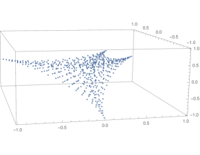
Figure 1: The common zeros of $T_{8,0,0},T_{0,8,0},T_{0,0,8}$.

In case of the symmetric group $S_{4}$ the general recurrence relation Prop. III, iv.) reads

$$\begin{split}&T_{j,k,p}\cdot T_{n,m,\ell}=\tfrac{1}{24}\mathopen{}\mathclose{{}\left(T_{\tiny\begin{pmatrix}-j+k+n\\ -j+m+p\\ l-j\end{pmatrix}}}\right.+T_{\tiny\begin{pmatrix}-j+k+n\\ -j+k+m-p\\ l-j\end{pmatrix}}\\ &+T_{\tiny\begin{pmatrix}-j+k+n\\ -j+m+p\\ l+p\end{pmatrix}}+T_{\tiny\begin{pmatrix}-j+k+n\\ -j+k+m-p\\ k+l-p\end{pmatrix}}+T_{\tiny\begin{pmatrix}-j+k+n\\ k+m\\ l+p\end{pmatrix}}\\ &+T_{\tiny\begin{pmatrix}-j+k+n\\ k+m\\ k+l-p\end{pmatrix}}+T_{\tiny\begin{pmatrix}-k+n+p\\ -j+m+p\\ l-j\end{pmatrix}}+T_{\tiny\begin{pmatrix}n-p\\ -j+k+m-p\\ l-j\end{pmatrix}}\\ &+T_{\tiny\begin{pmatrix}-k+n+p\\ -j+m+p\\ l+p\end{pmatrix}}+T_{\tiny\begin{pmatrix}n-p\\ -j+k+m-p\\ k+l-p\end{pmatrix}}+T_{\tiny\begin{pmatrix}-k+n+p\\ m-k\\ l-j\end{pmatrix}}\\ &+T_{\tiny\begin{pmatrix}n-p\\ m-k\\ l-j\end{pmatrix}}+T_{\tiny\begin{pmatrix}-k+n+p\\ m-k\\ j-k+l\end{pmatrix}}+T_{\tiny\begin{pmatrix}n-p\\ m-k\\ j-k+l\end{pmatrix}}\\ &+T_{\tiny\begin{pmatrix}-k+n+p\\ j-k+m+p\\ l+p\end{pmatrix}}+T_{\tiny\begin{pmatrix}n-p\\ j+m-p\\ k+l-p\end{pmatrix}}+T_{\tiny\begin{pmatrix}-k+n+p\\ j-k+m+p\\ j-k+l\end{pmatrix}}\\ &+T_{\tiny\begin{pmatrix}n-p\\ j+m-p\\ j-k+l\end{pmatrix}}+T_{\tiny\begin{pmatrix}j+n\\ k+m\\ l+p\end{pmatrix}}+T_{\tiny\begin{pmatrix}j+n\\ k+m\\ k+l-p\end{pmatrix}}+T_{\tiny\begin{pmatrix}j+n\\ j-k+m+p\\ l+p\end{pmatrix}}\\ &+T_{\tiny\begin{pmatrix}j+n\\ j+m-p\\ k+l-p\end{pmatrix}}+T_{\tiny\begin{pmatrix}j+n\\ j-k+m+p\\ j-k+l\end{pmatrix}}\mathopen{}\mathclose{{}\left.+T_{\tiny\begin{pmatrix}j+n\\ j+m-p\\ j-k+l\end{pmatrix}}}\right).\end{split}$$

This recurrence relation allows to derive the visualization of the signal model.

IV FFT algorithm for FCC cosine transform

IV-A The FCC cosine transform

We consider the signal model $M=\mathscr{A}=\mathbbm{C}[x,y,z]\big{/}\langle T_{n,0,0},T_{0,n,0},T_{0,0,n}\rangle$ with $\Phi\colon\mathbbm{C}^{n\times n\times n}\to M$ given as

$$s_{n,m,\ell}\mapsto s_{n,m,\ell}T_{n,m,\ell}.$$ (15)

Note that $b_{n}:=(T_{j,k,p}\;|\;0\leq j,k,p<n)$ is a basis of $M$. By Lemma 1 and (2) the signal space $M$ decomposes as

$$\begin{split}M\cong\bigoplus_{i,j,k}\mathbbm{C}[x,y,z]\big{/}&\langle x-x(u_{i},v_{j},w_{k}),\\ &y-y(u_{i},v_{j},w_{k}),\\ &z-z(u_{i},v_{j},w_{k})\rangle.\end{split}$$ (16)

The elements $T_{1,0,0},T_{0,1,0}$, and $T_{0,0,1}$ are the shifts of our signal model. If we multiply any element of $M$ by one of these, the element gets shifted into certain directions, as illustrated in Fig. 2(a). These resemble the roots of the Lie group $SU(4)$ and generate the FCC lattice. The convex hull of these shifts forms a rhombic dodecahedron, see Fig. 2(b). It fills the space by rescaling and placement on the lattice points. This can be easily seen, as the Voronoi cells of the FCC lattice are rhombic dodecahedra, cf. [1, Ch. 21, Sect. 3.B].

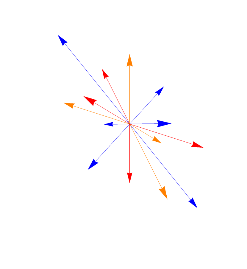
(a) The shifts $T_{1,0,0}$ (red), $T_{0,1,0}$ (blue), and $T_{0,0,1}$ (orange).

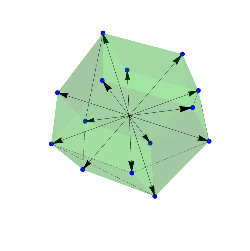
(b) Convex hull of the shifts, a rhombic dodecahedron.

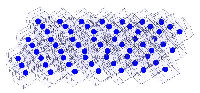
(c) Space-filling via rhombic dodecahedra on FCC lattice points.

Figure 2: The three variable Chebyshev polynomials give rise to shift operators. The rescaled convex hull of these shifts fills the whole space.

We now generalize our approach by introducing skew FCC cosine transforms. These are necessary, as we want to develop a divide-and-conquer approach for the algorithmic computation of the FCC cosine transform and they appear naturally in the derivation of the algorithm. For this, we introduce auxiliary functions

$$\sigma(r,s,t) :=\tfrac{1}{4}\mathopen{}\mathclose{{}\left(\mathrm{e}^{2\pi\mathrm{i}r}+\mathrm{e}^{2\pi\mathrm{i}(s-r)}+\mathrm{e}^{-2\pi\mathrm{i}t}+\mathrm{e}^{2\pi\mathrm{i}(t-s)}}\right),$$

$$\tau(r,s,t) :=\tfrac{1}{6}\mathopen{}\mathclose{{}\left(\mathrm{e}^{-2\pi\mathrm{i}s}+\mathrm{e}^{2\pi\mathrm{i}s}+\mathrm{e}^{2\pi\mathrm{i}(r-t)}+}\right.$$

$$\hskip 20.00003pt\mathopen{}\mathclose{{}\left.+\mathrm{e}^{2\pi\mathrm{i}(s-r-t)}+\mathrm{e}^{2\pi\mathrm{i}(t-r)}+\mathrm{e}^{2\pi\mathrm{i}(r-s+t)}}\right),$$

$$\rho(r,s,t) :=\tfrac{1}{4}\mathopen{}\mathclose{{}\left(\mathrm{e}^{-2\pi\mathrm{i}r}+\mathrm{e}^{2\pi\mathrm{i}(r-s)}+\mathrm{e}^{2\pi\mathrm{i}(s-t)}+\mathrm{e}^{2\pi\mathrm{i}t}}\right),$$

which yield the common zeros of $T_{1,0,0},T_{0,1,0}$, and $T_{0,0,1}$ in $(x,y,z)$-coordinates for $(r,s,t)=\mathopen{}\mathclose{{}\left(\tfrac{1}{8},0,\frac{3}{8}}\right)$, i.e. they are all equal to zero.

Consider the filter space $\mathscr{A}=\mathbbm{C}[x,y,z]\big{/}\langle T_{n,0,0}-\sigma(r,s,t),T_{0,n,0}-\tau(r,s,t),T_{0,0,n}-\rho(r,s,t)\rangle$ and the signal space $M=\mathscr{A}$. If we find a decomposition of the ideal $\langle T_{n,0,0}-\sigma(r,s,t),T_{0,n,0}-\tau(r,s,t),T_{0,0,n}-\rho(r,s,t)\rangle$ into coprime ideals, $M$ decomposes into one-dimensional spaces given by the factors of the ideal by the Chinese remainder theorem. The decomposition is achieved by finding the common zeros of the system of equations

$$T_{n,0,0}-\sigma(r,s,t) =0,$$

$$T_{0,n,0}-\tau(r,s,t) =0,$$ (17)

$$T_{0,0,n}-\rho(r,s,t) =0.$$

Inspecting the power form, we find the $n^{3}$ solutions for (17) in $(u,v,w)$-parameterization as $\{(\mathrm{e}^{2\pi\mathrm{i}\frac{r+i}{n}},\mathrm{e}^{2\pi\mathrm{i}\frac{s+j}{n}},\mathrm{e}^{2\pi\mathrm{i}\frac{t+k}{n}})\;|\;i,j,k=0,\dots,n-1\}$. Hence we get the decomposition:

Lemma 2.

For any $n$, we have

$$\begin{split}&\Big{\langle}T_{n,0,0}-\sigma(r,s,t),T_{0,n,0}-\tau(r,s,t),\\ &\quad T_{0,0,n}-\rho(r,s,t)\Big{\rangle}\\ &=\bigcap_{0\leq i,j,k<n}\Big{\langle}x-\sigma\mathopen{}\mathclose{{}\left(\tfrac{r+i}{n},\tfrac{s+j}{n},\tfrac{t+k}{n}}\right),\\ &\hskip 20.00003pty-\tau\mathopen{}\mathclose{{}\left(\tfrac{r+i}{n},\tfrac{s+j}{n},\tfrac{t+k}{n}}\right),z-\rho\mathopen{}\mathclose{{}\left(\tfrac{r+i}{n},\tfrac{s+j}{n},\tfrac{t+k}{n}}\right)\Big{\rangle},\end{split}$$ (18)

and as a consequence

$$\begin{split}&\mathbbm{C}[x,y,z]\Big{/}\Big{\langle}T_{n,0,0}-\sigma(r,s,t),T_{0,n,0}-\tau(r,s,t),\\ &\hskip 50.00008ptT_{0,0,n}-\rho(r,s,t)\Big{\rangle}\\ &\cong\bigoplus_{0\leq i,j,k<n}\mathbbm{C}[x,y,z]\Big{/}\Big{\langle}x-\sigma\mathopen{}\mathclose{{}\left(\tfrac{r+i}{n},\tfrac{s+j}{n},\tfrac{t+k}{n}}\right),\\ &\hskip 20.00003pty-\tau\mathopen{}\mathclose{{}\left(\tfrac{r+i}{n},\tfrac{s+j}{n},\tfrac{t+k}{n}}\right),z-\rho\mathopen{}\mathclose{{}\left(\tfrac{r+i}{n},\tfrac{s+j}{n},\tfrac{t+k}{n}}\right)\Big{\rangle}..\end{split}$$ (19)

We now can give the definition of the FCC cosine transform:

Definition .

The map realizing the isomorphism (19) is called the skew FCC cosine transform denoted by $\mathsf{DCT}_{n\times n\times n}(r,s,t)$. For $(r,s,t)=\mathopen{}\mathclose{{}\left(\tfrac{1}{8},0,\tfrac{3}{8}}\right)$, it is called the FCC cosine transform and is denoted by $\mathsf{DCT}_{n\times n\times n}$.

An explicit description of $\mathsf{DCT}_{n\times n\times n}$ in matrix form is given by inserting the common zeros of the Chebyshev polynomials $T_{n,0,0},T_{0,n,0}$, and $T_{0,0,n}$ into the Chebyshev polynomials of lower order, which form a basis of $M$:

$$\begin{split}&\mathsf{DCT}_{n\times n\times n}(r,s,t)\\ &=\bigg{(}T_{j,k,p}\mathopen{}\mathclose{{}\left(\sigma\mathopen{}\mathclose{{}\left(\tfrac{r+i}{n},\tfrac{s+\ell}{n},\tfrac{t+q}{n}}\right),\tau\mathopen{}\mathclose{{}\left(\tfrac{r+i}{n},\tfrac{s+\ell}{n},\tfrac{t+q}{n}}\right),}\right.\\ &\hskip 20.00003pt\mathopen{}\mathclose{{}\left.\rho\mathopen{}\mathclose{{}\left(\tfrac{r+i}{n},\tfrac{s+\ell}{n},\tfrac{t+q}{n}}\right)}\right)\bigg{)}_{0\leq i,j,k,\ell,p,q<n},\end{split}$$ (20)

where $(j,k,p)$ is the row index and $(i,\ell,q)$ the column index, both ordered lexicographically.

IV-B The Cooley-Tukey-type-algorithm for FCC $\mathsf{DCT}$

In this subsection we derive the fast radix-$2\times 2\times 2$ algorithm for the FCC cosine transform. Recall from [13, Sect. 3], that a recursive FFT algorithm can be deduced via stepwise decomposition of the signal space $M$. This procedure then gives a fast algorithm if the sample size $n$ is decomposable, e.g. $n=2^{k}$ for some $k$. Applying the stepwise composition for the case $n=2m$ yields

$$\mathbbm{C}[x,y,z]\big{/}$$ (21)

$$\langle T_{n,0,0}-\sigma(r,s,t),T_{0,n,0}-\tau(r,s,t),T_{0,0,n}-\rho(r,s,t)\rangle$$

$$\longrightarrow \mathbbm{C}[x,y,z]\big{/}$$ (22)

$$\hskip 20.00003pt\big{\langle}T_{2,0,0}(T_{m,0,0},T_{0,m,0},T_{0,0,m})-\sigma(r,s,t),$$

$$\hskip 20.00003ptT_{0,2,0}(T_{m,0,0},T_{0,m,0},T_{0,0,m})-\tau(r,s,t),$$

$$\hskip 20.00003ptT_{0,0,2}(T_{m,0,0},T_{0,m,0},T_{0,0,m})-\rho(r,s,t)\big{\rangle}$$

$$\longrightarrow \bigoplus_{i_{r},i_{s},i_{t}=0,1}\mathbbm{C}[x,y,z]\big{/}$$ (23)

$$\hskip 20.00003pt\Big{\langle}T_{m,0,0}-\sigma\mathopen{}\mathclose{{}\left(\tfrac{r+i_{r}}{2},\tfrac{s+i_{s}}{2},\tfrac{t+i_{t}}{2}}\right),$$

$$\hskip 20.00003ptT_{0,m,0}-\tau\mathopen{}\mathclose{{}\left(\tfrac{r+i_{r}}{2},\tfrac{s+i_{s}}{2},\tfrac{t+i_{t}}{2}}\right),$$

$$\hskip 20.00003ptT_{0,0,m}-\rho\mathopen{}\mathclose{{}\left(\tfrac{r+i_{r}}{2},\tfrac{s+i_{s}}{2},\tfrac{t+i_{t}}{2}}\right)\Big{\rangle}$$

$$\longrightarrow \bigoplus_{i_{r},i_{s},i_{t}=0,1\,}\bigoplus_{\,k_{r},k_{s},k_{t}=0,\dots,m-1}\mathbbm{C}[x,y,z]\big{/}$$ (24)

$$\hskip 20.00003pt\Big{\langle}x-\sigma\mathopen{}\mathclose{{}\left(\tfrac{r+i_{r}+2k_{r}}{n},\tfrac{s+i_{s}+2k_{s}}{n},\tfrac{t+i_{t}+2k_{t}}{n}}\right),$$

$$\hskip 20.00003pty-\tau\mathopen{}\mathclose{{}\left(\tfrac{r+i_{r}+2k_{r}}{n},\tfrac{s+i_{s}+2k_{s}}{n},\tfrac{t+i_{t}+2k_{t}}{n}}\right),$$

$$\hskip 20.00003ptz-\rho\mathopen{}\mathclose{{}\left(\tfrac{r+i_{r}+2k_{r}}{n},\tfrac{s+i_{s}+2k_{s}}{n},\tfrac{t+i_{t}+2k_{t}}{n}}\right)\Big{\rangle}$$

$$\longrightarrow \bigoplus_{j_{r},j_{s},j_{t}=0,\dots,n-1}\mathbbm{C}[x,y,z]\big{/}$$ (25)

$$\hskip 20.00003pt\Big{\langle}x-\sigma\mathopen{}\mathclose{{}\left(\tfrac{r+j_{r}}{n},\tfrac{s+j_{s}}{n},\tfrac{t+j_{t}}{n}}\right),$$

$$\hskip 20.00003pty-\tau\mathopen{}\mathclose{{}\left(\tfrac{r+j_{r}}{n},\tfrac{s+j_{s}}{n},\tfrac{t+j_{t}}{n}}\right),z-\rho\mathopen{}\mathclose{{}\left(\tfrac{r+j_{r}}{n},\tfrac{s+j_{s}}{n},\tfrac{t+j_{t}}{n}}\right)\Big{\rangle}.$$

Each step is encoded by a matrix. We have for (22) a complicated basis change matrix $B_{n}(r,s,t)$. We go from the old basis $b_{n}$ ordered lexicographically to the new basis

$$\widetilde{b}_{n}:=\begin{bmatrix}T_{0,0,0}T_{0,0,0}(T_{m,0,0},T_{0,m,0},T_{0,0,m})\\ \vdots\\ T_{m-1,m-1,m-1}T_{1,1,1}(T_{m,0,0},T_{0,m,0},T_{0,0,m})\end{bmatrix}.$$

This basis change, which has $O(n^{3})$ entries, will be described in future works. For (23) we apply the matrix $\mathsf{DCT}_{2\times 2\times 2}(r,s,t)\mathbin{\otimes}\mathbbm{1}_{m^{3}}$, for (24) we obtain the recursion steps via the application of $\bigoplus_{i_{r},i_{s},i_{t}=0,1}\mathsf{DCT}_{m\times m\times m}\mathopen{}\mathclose{{}\left(\frac{r+i_{r}}{2},\frac{s+i_{s}}{2},\frac{t+i_{t}}{2}}\right)$. Finally we get a permutation matrix $P_{n}$ in (25). The fast algorithm is given as the matrix factorization

$$\begin{split}&\mathsf{DCT}_{n\times n\times n}(r,s,t)\\ &=P_{n}\cdot\bigoplus_{i_{r},i_{s},i_{t}=0,1}\mathsf{DCT}_{m\times m\times m}\mathopen{}\mathclose{{}\left(\tfrac{r+i_{r}}{2},\tfrac{s+i_{s}}{2},\tfrac{t+i_{t}}{2}}\right)\\ &\quad\cdot(\mathsf{DCT}_{2\times 2\times 2}(r,s,t)\mathbin{\otimes}\mathbbm{1}_{m^{3}})\cdot B_{n}(r,s,t).\end{split}$$ (26)

Looking at the matrix representation makes it easy to see that the whole algorithm has cost $O(n^{3}\log(n))$. Hence it can compete with the tensor product of standard Cooley-Tukey FFTs or fast Cosine transforms. First numerical experiments verify the effectivity of the proposed methodology compared to the naive $O(n^{6})$ implementation, as depicted in Fig. 3.

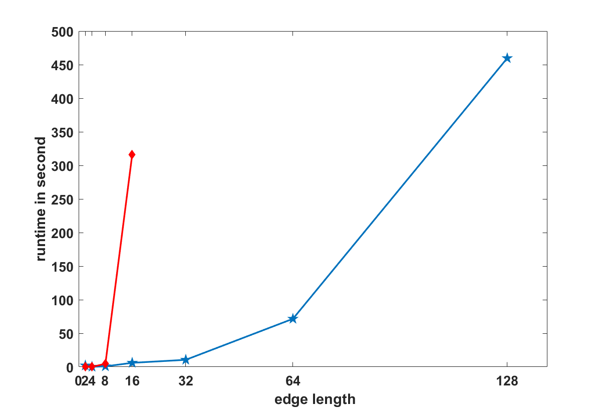
Figure 3: Runtime of a naive $O(n^{6})$ implementation (red diamonds) and the fast $O(n^{3}\log(n))$ algorithm (blue pentagrams).

V Application to voxel data and future work

One of the main advantages of using the algebraic signal model is that we do not actually have to sample data on the FCC lattice, but can instead use the $z$-transform to map any data on it. Hence we can compare the effect of the FCC transform directly with the standard approach to discrete cosine transforms on cc lattices.

For graphic representation of voxel data on a rectangular grid, each data point gets assigned to a cuboid and can define certain properties, like color or opacity. Now for the FCC lattice we have to assign the points to rhombic dodecahedra instead, as they fill the space on this lattice. The difference in the graphical representation is shown in Fig 4, where we created an artifical data set portraying a sword. The data values were mapped to opacity values, i.e. data points with value $0$ are not visible, while the ones with $1$ are fully visible.

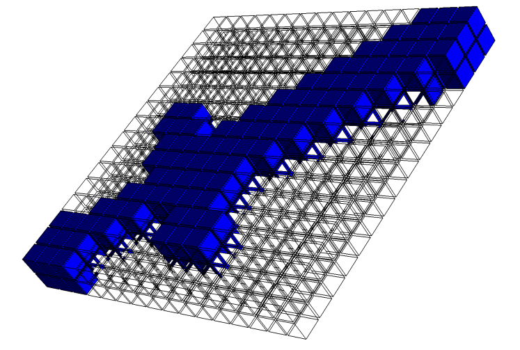
(a) Sword represented via cuboids.

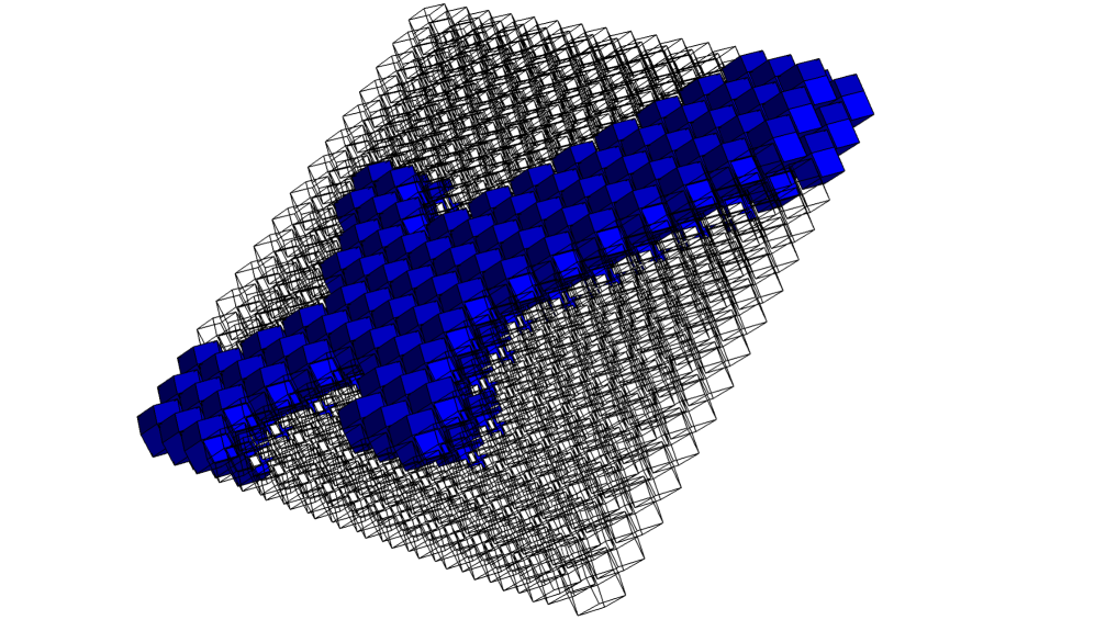
(b) Sword represented via rhombic dodecahedra.

Figure 4: Data representation on a rectangular grid and on a $SU(4)$ grid.

In Fig. 5(a) we see the effect of the threefold tensor product of the discrete cosine transform and in Fig. 5(b) the effect of the FCC Chebyshev transform.

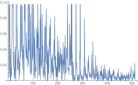
(a) The threefold discrete cosine spectrum of the sword on a CC lattice.

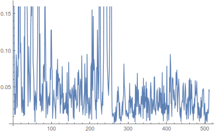
(b) The $\mathsf{DCT}$ spectrum of the sword on a FCC lattice.

Figure 5: Spectra of the Sword.

Aside from an explicit description of the matrices used in the decomposition steps, we plan to derive Cooley-Tukey-type-algorithms based on generalized Chebyshev polynomials for all simple, compact Lie groups.

References

- [1] J. Conway and N. Sloane, Sphere Packings, Lattices and Groups, 3rd ed. Springer, 1999.
- [2] V. Vad, B. Csébfalvi, and E. Rautek, P.and Gröller, “Towards an unbiased comparison of cc, bcc, and fcc lattices in terms of prealiasing,” Comput. Graph. Forum, vol. 33, no. 3, pp. 81–90, 2014.
- [3] H. R. Künsch, E. Agrell, and F. A. Hamprecht, “Optimal lattices for sampling,” IEEE Trans. Inf. Theory, vol. 51, no. 2, pp. 634–647, 2005.
- [4] M. Mirzargar and A. Entezari, “Voronoi Splines,” IEEE Transactions on Signal Processing, vol. 58, no. 9, pp. 4572–4582, 2010.
- [5] T. Meng, A. Entezari, B. Smith, T. Möller, D. Weiskopf, and A. Kirkpatrick, “Visual comparability of 3D regular sampling and reconstruction,” IEEE Trans. Vis. Comput. Graphics, vol. 17, no. 10, pp. 1420–1432, 2011.
- [6] M. Saranathan, V. Ramanan, R. Gulati, and R. Venkatesan, “ANTHEM: anatomically tailored hexagonal MRI,” Magn. Reson. Imag., vol. 25, no. 7, pp. 1039–1047, 2007.
- [7] D. P. Petersen and D. Middleton, “Sampling and reconstruction of wave-number-limited functions in -dimensional Euclidean space,” Inf. Control, vol. 5, no. 4, pp. 279–323, 1962.
- [8] R. M. Mersereau and T. C. Speake, “A unified treatmen of Cooley-Tukey algorithms for the evaluation of the multidimensional DFT,” IEEE Trans. Acoust., Speech, Signal Process., vol. 29, no. 5, pp. 1011–1018, 1981.
- [9] X. Zheng and F. Gu, “Fast Fourier Transform on FCC and BCC Lattices with Outputs on FCC and BCC Lattices Respectively,” J Math Imaging Vis, vol. 49, no. 3, pp. 530–550, 2014.
- [10] M. Püschel and J. Moura, “Algebraic signal processing theory: Foundation and 1-D time,” Signal Processing, IEEE Trans., vol. 56, no. 8, pp. 3572–3585, 2008.
- [11] ——, “The algebraic approach to the discrete cosine and sine transforms and their fast algorithms,” SIAM J. Comput., vol. 32, no. 5, pp. 1280–1316, 2003.
- [12] ——, “Algebraic signal processing theory: Cooley-Tukey type algorithms for DCTs and DSTs,” Signal Processing, IEEE Trans., vol. 56, no. 4, pp. 1502–1521, 2008.
- [13] M. Püschel and M. Rötteler, “Algebraic signal processing theory: Cooley-Tukey type algorithms on the 2-D hexagonal spatial lattice,” Applicable Algebra in Engineering, Communication and Computing, vol. 19, no. 3, pp. 259–292, 2008.
- [14] M. Azam, M. A. Anjum, and M. Y. Javed, “Discrete cosine transform (dct) based face recognition in hexagonal images,” in 2010 The 2nd International Conference on Computer and Automation Engineering (ICCAE), vol. 2, 2010, pp. 474–479.
- [15] M. E. Hoffman and W. D. Withers, “Generalized Chebyshev polynomials associated with affine Weyl groups,” Trans. Amer. Math. Soc., vol. 308, pp. 91–104, 1988.
- [16] B. N. Ryland and H. Munthe-Kaas, “On multivariate Chebyshev polynomials and spectral approximations on triangles,” in Spectral and High Order Methods for Partial Differential Equations, J. S. Hesthaven and E. M. Ronquist, Eds. Springer, 2011, pp. 19–41.
- [17] H. Munthe-Kaas, M. Nome, and B. N. Ryland, “Through the kaleidoscope: Symmetries, groups and Chebyshev-approximations from a computational point of view,” in Foundations of Computational Mathematics, Budapest 2011, F. Cucker, T. Krick, A. Pinkus, and A. Szanto, Eds. Cambridge Universtiy Press, 2012, pp. 188–229.
- [18] H. Li and Y. Xu, “Discrete Fourier analysis on fundamental domain and simplex of lattice in -variables,” J Fourier Anal Appl, vol. 16, pp. 383–433, 2010.
- [19] R. V. Moody and J. Patera, “Cubature formulae for orthogonal polynomials in terms of elements of finite order of compact simple Lie groups,” Adv. Appl. Math., vol. 47, pp. 509–535, 2011.
- [20] J. Hrivnák, L. Motlochová, and J. Patera, “Cubature formulas of multivariate polynomials arising from symmetric orbit functions,” Symmetry, vol. 8, p. 63, 2016.
- [21] A. Atoyan and J. Patera, “The discrete transform and its continuous extension for triangular lattices,” J. Geometry Phys., vol. 57, pp. 745–764, 2007.
- [22] W. Adams and P. Loustaunau, An Introduction to Gröbner Bases. American Mathematical Society, 1994.
- [23] P. E. Ricci, “Una proprietà iterativa dei polinomi di Chebyshev di prima specie in più variabili,” Rendiconti di matematica e delle sue applicazioni, vol. 6, pp. 555–563, 1986.