Multicritical Scaling in a Lattice Model of Vesicles

Abstract

Vesicles, or closed fluctuating membranes, have been modeled in two dimensions by self-avoiding polygons, weighted with respect to their perimeter and enclosed area, with the simplest model given by area-weighted excursions. These models generically show a tricritical phase transition between an inflated and a crumpled phase, with a scaling function given by the logarithmic derivative of the Airy function. Extending such a model, we find realizations of multicritical points of arbitrary order, with the associated multivariate scaling functions expressible in terms of generalized Airy integrals, as previously conjectured by John Cardy. This work therefore adds to the small list of models with a critical phase transition, for which exponents and the associated scaling functions are explicitly known.

Introduction.—Obtaining a thorough understanding of phase transitions is one of the main aims of statistical physics. For a continuous transition one would like to know the critical exponents describing the singular power-law behaviour of thermodynamic quantities as the transition is approached. Moreover, in the vicinity of such a transition it is generally believed that the thermodynamic quantities depend only on a suitably scaled combination of the parameters in terms of a universal scaling function Cardy (1996). Most progress has been made in two dimensions with the help of conformal invariance Henkel (2013). While these scaling functions can be easily obtained numerically, there are only few instances for which one knows precise expressions, one classical example being the spin-spin correlations of the two-dimensional Ising model Wu et al. (1976). Based on field-theoretic arguments, John Cardy postulated that by including many-body interactions in a model of vesicles, a hierarchy of scaling functions could be found, expressed in terms of generalized, higher-order Airy integrals

$$\Theta_{\ell}(s_{1},s_{2},\dots,s_{\ell})=\frac{1}{2\pi i}\int_{C}\exp\left(\frac{u^{\ell+2}}{\ell+2}-\sum_{j=1}^{\ell}s_{j}u^{j}\right)du,$$ (1)

with a suitable contour $C$. However, he cautioned that due to the technical limitations of the method used, “it is very difficult to say to what these higher multicritical points might correspond physically” Cardy (2001). In this letter, we give explicit examples of a statistical mechanical model having precisely these scaling functions, thereby providing a resolution to this problem.

Vesicles and Self-Avoiding Polygons.—A vesicle consists of a closed membrane formed from a lipid bilayer inside a watery solution. Depending on parameters such as the temperature and the osmotic pressure difference between the outside and the inside of the membrane, vesicles are found in different typical conformations Seifert (1997). Subject to thermal fluctuations, a vesicle of fixed surface area favours “crumpled” configurations with relatively small volume if there is a large net pressure acting onto the outside of the membrane. On the other hand, if there is a net pressure acting onto the inside of the membrane, then the vesicle tends to appear in an inflated shape with larger volume.

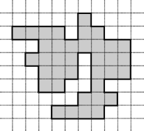
In Leibler et al. (1987), a two-dimensional model of vesicles was proposed in terms of ring polymers enclosing an area. In this case, the length of the polymer plays the role of the surface area of the vesicle, and the volume of the vesicle becomes the enclosed area. In Banavar et al. (1991); Fisher et al. (1991) the vesicles were modeled as self-avoiding polygons (SAP) on the square lattice – see Fig. 1 for an example. Note that any intrinsic property of the vesicle membrane such as stiffness is neglected in that lattice model.

Figure 1: A self-avoiding polygon (SAP) on $\mathbb{Z}^{2}$ of perimeter 52 and area 37.

In order to analyze the model of SAP, one defines the area-perimeter generating function

$$P(x,q)=\sum_{m=0}^{\infty}\sum_{n=0}^{\infty}p_{m,n}x^{m}q^{n},$$ (2)

where $p_{m,n}$ is the number of SAP with perimeter $m$ and area $n$, with two SAP being considered identical if they are the same up to translation. The qualitative behaviour of the radius of convergence $q_{c}(x)$ of $G(x,q)$, seen as a series in $q$ for fixed values of $x$, was discussed in Fisher et al. (1991); Banavar et al. (1991). This quantity is closely related to the asymptotic growth rate of the partition function $Z_{n}(x)=\sum_{m=0}^{\infty}p_{m,n}x^{m}$, and thus physically to the free energy per unit area in the thermodynamic limit of infinite area. This model exhibits a phase transition at a value $x_{c}$ at which $q_{c}(x)$ is not analytic. More precisely, it was shown that there exists a value $x_{c}>0$ such that for $0\leq x\leq x_{c}$, $q_{c}(x)=1$; for $x>x_{c}$, $q_{c}(x)$ is a continuous function of $x$, $q_{c}(x)<1$ and $\lim_{x\to\infty}q_{c}(x)=0$ – see Fig. 2. For $q<q_{c}(x)$, polygons with relatively small area dominate the sum (2). This part of the $(x,q)$-plane is called the droplet phase. Analogously, the region $q>1$ is labeled the inflated phase. The region where $q_{c}(x)<q<1$ is described as the ‘seaweed’ phase, in which the typical conformation consists of a space-filling, convoluted polygon. Exact enumerations yield the estimate $x_{c}\simeq 0.379$ Jensen and Guttmann (1999). The point $(x,q)=(x_{c},1)$ is called a tricritical point Lawrie and Sarbach (1984).

Figure 2: Qualitative picture of the phase diagram of the SAP model of vesicles. The line $q_{c}(x)$ is the boundary of the droplet phase. The exponents $\gamma,\theta$ and $\phi$ characterize the singular behaviour of the generating function $P(x,q)$ around the tricritical point.

In Richard et al. (2001, 2004), exact enumeration data was used to analyse the singular behaviour of the area-perimeter generating function of rooted SAP. In rooted SAP, there exists one distinguished point on the perimeter of the SAP, therefore the number of rooted SAP with perimeter $m$ and area $n$ is $mp_{m,n}$, and the area-perimeter generating function is $R(x,q)=x\frac{d}{dx}P(x,q)$. It was conjectured that in the vicinity of the point $(x,q)=(x_{c},1)$, the singular part of this function satisfies the scaling relation

$$R^{\operatorname{sing}}\left(x,e^{-\epsilon}\right)=\epsilon^{\theta}F((x_{c}-x)\epsilon^{-\phi}),$$ (3)

with the scaling function being, up to prefactors, given by the logarithmic derivative of the Airy function, which is defined for $z\in\mathbb{C}$ as DLMF

$$\operatorname{Ai}(z)=\frac{1}{2\pi i}\int_{\infty e^{-i\pi/3}}^{\infty e^{i\pi/3}}\exp\left(\frac{u^{3}}{3}-zu\right)du.$$ (4)

In Cardy (2001) it was argued via field theoretic methods that, upon introducing further interactions into the SAP model, one should be able to observe multicritical points of higher order, described by scaling functions of more than one variable. More precisely, upon introducing $\ell-1$ further interactions $(w_{j})_{j=1}^{\ell-1}$, there should exist multicritical points in the vicinity of which the singular part of the multivariate generating function of rooted SAP satisfies the scaling relation

$$R^{sing}(w_{1},\dots,w_{\ell-1},x,q)=\epsilon^{\theta}F(\alpha_{1}\epsilon^{\phi_{1}},\alpha_{2}\epsilon^{\phi_{2}},\dots,\alpha_{\ell}^{\phi_{\ell}}),$$ (5)

where the variables $(\alpha_{j})_{j=1}^{\ell}$ depend on the parameters of the generating function, the crossover exponents $\phi_{j}$ are given by

$$\phi_{j}=\phi_{j}(\ell)=\frac{\ell+2-j}{\ell+2}\quad(1\leq j\leq\ell),$$ (6)

and $\theta=\frac{1}{\ell+2}$ is a critical exponent. The scaling function $F(s_{1},s_{2},\dots,s_{\ell})$ is expressible in terms of generalized, higher-order Airy integrals, defined in Eq. (1). However, no details of the interactions necessary to observe these multicritical points were given in that reference.

The Model.—One-dimensional lattice paths occur in many applications in probability theory, combinatorics and statistical physics. For $m\in\mathbb{N}_{0}=\mathbb{N}\cup\{0\}$, a one-dimensional lattice path of length $m$ is a sequence $(\mathbf{r}_{0},\mathbf{r}_{2},\dots,\mathbf{r}_{m})$ of points of $\mathbb{Z}^{2}$, where for $0<j\leq m$, $\mathbf{r}_{j}-\mathbf{r}_{j-1}\in\{1\}\times\mathcal{S}$, with $\mathcal{S}\subseteq\mathbb{Z}$ Banderier and Flajolet (2002). One usually fixes $\mathbf{r}_{0}=(0,0)$. The path then stays in the right half-plane. Paths restricted further to stay in the upper right quarter plane $\mathbb{N}_{0}\times\mathbb{N}_{0}$ are called meanders, paths which end on the horizontal line $\mathbb{N}_{0}\times\{0\}$ are called bridges, and paths which are both meanders and bridges are called excursions. Łukasiewicz paths, which encode rooted ordered trees Le Gall (2005), are excursions with $\mathcal{S}=\{k\in\mathbb{Z}\leavevmode\nobreak\ |\leavevmode\nobreak\ k\geq-1\}$. Excursions with $\mathcal{S}=\{-1\}\,\cup\,\{j\leavevmode\nobreak\ |\leavevmode\nobreak\ k\leq j\leq\ell\}$, where $k,\ell\in\mathbb{N}_{0}$, are called $(k,\ell)$-Łukasiewicz paths Brak et al. (2011).

Figure 3: A $(1,3)$-Łukasiewicz path of length 13.

Figure 3 shows a $(1,3)$-Łukasiewicz path of length 13, with the horizontal and vertical axes of $\mathbb{Z}^{2}$ labeled by $x$ and $y$, respectively. A step in the direction $(1,-1)$ is called a down-step and a step in direction $(1,k)$, where $k\geq 1$ is called an up-step of length $k$. The height of a point is its distance from the $x$-axis, and the height of a step is the height of its initial point. The initial points of the up-steps in Fig. 3 are marked by red dotted lines. Special subclasses of Łukasiewicz paths are Dyck and Motzkin paths, corresponding to $(k,\ell)=(1,1)$ and $(k,\ell)=(0,1)$, respectively.

In this letter we consider the generating function

$$G_{\ell}(\mathbf{w},x,q)=\sum_{m,j_{1},\ldots,j_{\ell}}c(j_{1},\dots,j_{\ell},m,n)w_{1}^{j_{1}}\dots w_{\ell}^{j_{\ell}}x^{m}q^{n},$$ (7)

where we abbreviate $w_{1},\dots,w_{\ell}=\mathbf{w}$ and where $c(j_{1},\dots,j_{\ell},m,n)$ is the number of $(1,\ell)$-Łukasiewicz paths with $m$ up-steps, of which $j_{1}$ have length one, $j_{2}$ have length two etc., and the sum of the heights of all the up-steps is $n$, which is an area-like quantity (in the case of Dyck paths, the number of lattice points below the path is precisely $2n+m$). For example, the path shown in Fig. 3 has the weight $w_{1}^{3}w_{2}w_{3}x^{5}q^{5}$ in the generating function $G_{3}(w_{1},w_{2},w_{3},x,q)$. One can set $w_{1}=1$ without loss of generality. In the following we therefore write $G_{\ell}(1,w_{2},\dots,w_{\ell},x,q)\equiv G_{\ell}(w_{2},\dots,w_{\ell},x,q)$.

Previous Results.—In Haug and Prellberg (2015), the asymptotic behaviour of $G_{1}(x,q)$ in the limit $q\to 1^{-}$ was analysed, despite the parameters being interpreted slightly differently there. In particular it was shown that, in the vicinity of the tricritical point $(x,q)=(\frac{1}{4},1)$, the singular part of the generating function satisfies the scaling relation

$$G_{1}^{\operatorname{sing}}\left(x,e^{-\epsilon}\right)=\epsilon^{\theta}F((x_{c}-x)\epsilon^{-\phi}),$$ (8)

where $\theta=\frac{1}{3}$, $\phi=\frac{2}{3}$ and $F(s)=b_{0}\frac{d}{ds}\ln(\operatorname{Ai}(b_{1}s))$, with positive constants $b_{0}$ and $b_{1}$. Consistently with the solution $G_{1}(x,1)=\frac{1}{2x}(1-\sqrt{1-4x})$, Eq. 8 implies with the asymptotic expansions of the Airy function and its derivative DLMF that $G_{1}^{\operatorname{sing}}(x,1)\sim 2(x_{c}-x)^{\gamma}$, where $\gamma=\frac{\theta}{\phi}=\frac{1}{2}$. Up to different constants $b_{0}$ and $b_{1}$, the scaling relation (8) is identical to the one in Eq. (3) that was conjectured to hold for rooted self-avoiding polygons.

Result.—In Haug et al. (2017), it was shown rigorously that around the multicritical point $(w_{2},x,q)=(-\frac{1}{9},\frac{1}{3},1)$, the singular part of $G_{2}(w_{2},x,q)$ satisfies the scaling relation

$$G^{\operatorname{sing}}_{2}(w_{2},x,q)=\epsilon^{\theta}F(\alpha_{1}\epsilon^{-\phi_{1}},\alpha_{2}\epsilon^{-\phi_{2}}),$$ (9)

where the scaling variables $\alpha_{1}$ and $\alpha_{2}$ are analytic functions of $w_{2}$ and $x$, $\theta=\frac{1}{4},\phi_{1}=\frac{3}{4},\phi_{2}=\frac{1}{2}$, and the scaling function $F$ is expressible via $\Theta_{2}(s_{1},s_{2})$.

This result is generalized in this letter. More specifically, we show that for arbitrary $\ell\geq 2$, there exists a multicritical point $(w_{2},\dots,w_{\ell},x,q)$ in the model of $(1,\ell)$-Łukasiewicz paths, with $x=(\ell+1)^{-1},q=1$ and

$$w_{k}=\frac{2}{\ell(\ell+1)}\left(\frac{-1}{\ell+1}\right)^{k-1}{\ell+1\choose k+1}\quad(2\leq k\leq\ell),$$ (10)

in the vicinity of which the generating function $G_{\ell}(w_{2},\dots,w_{\ell},x,q)$ satisfies a scaling relation of the form of Eq. 5 with the same scaling function and the same critical exponents as predicted in Cardy (2001). We thus present an exactly solvable model representing a concrete realization of the multicritical scaling postulated in that reference.

Method.—To obtain an asymptotic expression for $G_{\ell}(w_{2},\dots,w_{\ell},x,q)$ in the limit $q\to 1^{-}$ for arbitrary $\ell\geq 2$, one proceeds analogously to Haug and Prellberg (2015); Haug et al. (2017). From a simple factorization argument Brak et al. (2011) one obtains the functional equation

$$G_{\ell}(\mathbf{w},x,q)=1+xG_{\ell}(\mathbf{w},x,q)\left(\sum_{k=1}^{\ell}w_{k}\prod_{j=1}^{k}G_{\ell}(\mathbf{w},q^{j}x,q)\right).$$ (11)

We linearize Eq. 11 by using the ansatz

$$G_{\ell}(w_{2},\dots,w_{\ell},x,q)=\frac{\Phi(qx)}{\Phi(x)},$$ (12)

where $\Phi(x)\equiv\Phi(w_{2},\dots,w_{\ell},x,q)$, The solution of the linearized equation is then given by the $q$-hypergeometric series Gasper and Rahman (1990)

$$\Phi(x)=\sum_{n=0}^{\infty}\frac{\prod_{j=1}^{\ell-1}(\omega_{j};q)_{n}}{(q;q)_{n}}(-x)^{n}q^{n^{2}-n},$$ (13)

where $(z;q)_{n}=\prod_{j=0}^{n-1}(1-zq^{j})$ is the $q$-Pochhammer symbol and the parameters $(\omega_{k})_{k=1}^{\ell-1}$ satisfy

$$w_{k}=\frac{(-1)^{k}}{k!}\sum_{j_{1}=1}^{\ell-1}\sum_{j_{2}=1}^{\ell-1}\cdots\sum_{j_{k-1}=1}^{\ell-1}\prod_{p=1}^{k-1}\omega_{j_{p}}\quad(1\leq k\leq\ell).$$ (14)

Using the identity

$$\frac{(-1)^{n+1}q^{{n\choose 2}}}{(q;q)_{n}(q;q)_{\infty}}=\operatorname{Res}\left[(z;q)_{\infty}^{-1};z=q^{-n}\right],$$ (15)

we obtain for $k\in\mathbb{Z}$ the integral expression

$$\Phi(q^{k}x)=\frac{A}{2\pi i}\int_{C}\frac{z^{\frac{1}{2}(\log_{q}(z)+1)-\log_{q}(x)}}{z^{k}\left(\prod_{j=1}^{\ell-1}(\omega_{j}/z;q)_{\infty}\right)(z;q)_{\infty}}dz,$$ (16)

where the prefactor $A$ is independent of $k$, and $C$ is a suitably chosen complex contour. Substituting an asymptotic expression for the $q$-Pochhammer symbol Prellberg (1995), the above integral satisfies

$$\Phi(q^{k}x)\sim\frac{A}{2\pi i}\int_{C}\exp\left(\frac{1}{\epsilon}f(z)\right)\frac{g(z)}{z^{k}}dz\quad(q=e^{-\epsilon}\to 1^{-}),$$ (17)

where the functions are

$$f(z) =\log(x)\log(z)-\frac{\log(z)^{2}}{2}+\sum_{j=1}^{\ell-1}\operatorname{Li}_{2}\left(\frac{\omega_{j}}{z}\right),$$ (18)

$$g(z) =\left(\frac{z^{\ell}}{(1-z)\prod_{j=1}^{\ell-1}(z-\omega_{j})}\right)^{\frac{1}{2}},$$ (19)

and where $\operatorname{Li}_{2}(z)$ is the Euler dilogarithm DLMF . The saddle points of $f(z)$ are the zeros of the polynomial

$$\chi(z) =x\left(\prod_{j=1}^{\ell-1}z-\omega_{j}\right)-z^{\ell}(1-z)$$ (20)

$$=z^{\ell+1}\left(1-\frac{1}{z}+\frac{x}{z}\sum_{j=1}^{\ell}\frac{w_{j}}{z^{j}}\right)\quad(z\neq 0).$$

Comparing the bracket in the last expression with Eq. 11, we see that the solution of Eq. 11 for $q=1$ is equal to the inverse of a saddle point of $f(z)$. If we set the weights for $2\leq k\leq\ell$ to the ones given in Eq. 10, then $\ell+1$ saddle points coalesce in the point $z=(\ell+1)^{-1}$ for $x=(\ell+1)^{-1}$. To obtain an asympotic expression for $\Phi(q^{k}x)$, we apply a method devised in Ursell (1972), based on a theorem from Levinson (1961), from which it follows that if the parameters of the function $f(z)$ are close to the critical values given in Eq. 10, then there exists a mapping $\operatorname{T}:u\mapsto z(u)$, which is analytic and bijective in the vicinity of the point $z=(\ell+1)^{-1}$, such that

$$f(z(u))=\frac{u^{\ell+2}}{\ell+2}-\sum_{j=0}^{\ell}\alpha_{j}u^{j}=p(u).$$ (21)

Moreover, the coefficients $(\alpha_{j})_{j=0}^{\ell}$ are analytic functions of $(w_{j})_{j=2}^{\ell}$ and $x$ in the region around the point of coalescence of the saddle points. Using the transformation $\operatorname{T}$, the integral in Eq. 17 can be rewritten as

$$\Phi(q^{k}x)=\frac{A}{2\pi i}\int_{C^{\prime}}\exp\left(\frac{1}{\epsilon}\left[\frac{u^{\ell+2}}{\ell+2}-\sum_{j=0}^{\ell}\alpha_{j}u^{j}\right]\right)S_{k}(u)du\;,$$ (22)

where $q=e^{-\epsilon}\to 1^{-}$, $C^{\prime}$ is the image of the contour $C$ under $\operatorname{T}^{-1}$ and $S_{k}(u)=\frac{g(z(u))}{z(u)^{k}}\frac{dz}{du}$. Now one writes

$$S_{k}(u)=\sum_{j=0}^{\ell}p_{j}^{(k)}u^{k}+p^{\prime}(u)H(u),$$ (23)

where the $(p_{j}^{(k)})_{j=0}^{\ell}$ are analytic functions of the $(w_{j})_{j=2}^{\ell}$ and $x$, and $H(u)$ is some analytic function of $u$. Substituting Eq. 23 into Eq. 22, one arrives at the asymptotic expression

$$\Phi(q^{k}x) =$$ (24)

$$A\sum_{j=0}^{\ell}p_{j}^{(k)}\epsilon^{\frac{j}{\ell+2}}\Theta_{\ell}^{(j)}(\alpha_{1}\epsilon^{-\frac{\ell+1}{\ell+2}},\alpha_{2}\epsilon^{-\frac{\ell}{\ell+2}},\dots,\alpha_{\ell}\epsilon^{-\frac{2}{\ell+2}}),$$

where $\Theta_{\ell}^{(0)}=\Theta_{\ell}$ and $\Theta_{\ell}^{(j)}=-\frac{\partial}{\partial s_{j}}\Theta_{\ell}$ for $1\leq j\leq\ell$. By substituting Eq. 24 into Eq. 12 for $k=0$ and $k=1$, we obtain an asymptotic expression for $G_{\ell}(w_{2},\dots,w_{\ell},x,q)$ which is valid uniformly with respect to the parameters $(w_{j})_{j=2}^{\ell}$ and $x$, in particular in the vicinity of the multicritical point at which $\ell+1$ saddle points of the function $f(z)$ coalesce. Close to the multicritical point, the singular part of $G_{\ell}(w_{2},\dots,w_{\ell},x,q)$ satisfies the scaling relation

$$G^{\operatorname{sing}}_{\ell}(w_{2},\dots,w_{\ell},x,e^{-\epsilon})=\epsilon^{\theta}F(\alpha_{1}\epsilon^{-\phi_{1}},\dots,\alpha_{\ell}\epsilon^{-\phi_{\ell}}),$$ (25)

where $F$ is expressible via $\Theta_{\ell}(s_{1},\dots,s_{\ell})$, $\theta=\frac{1}{\ell+2}$, and the $\phi_{j}\equiv\phi_{j}(\ell)$ are given by Eq. 6.

References

- Cardy (1996) J. Cardy, Scaling and renormalization in statistical physics, Cambridge Lecture Notes in Physics (Cambridge University Press, 1996).
- Henkel (2013) M. Henkel, Conformal invariance and critical phenomena (Springer Science & Business Media, 2013).
- Wu et al. (1976) T. T. Wu, B. M. McCoy, C. A. Tracy, and E. Barouch, Phys. Rev. B 13, 316 (1976).
- Cardy (2001) J. Cardy, Journal of Physics A: Mathematical and General 34, L665 (2001).
- Seifert (1997) U. Seifert, Advances in Physics 46, 13 (1997).
- Leibler et al. (1987) S. Leibler, R. R. P. Singh, and M. E. Fisher, Physical Review Letters 59, 1989 (1987).
- Banavar et al. (1991) J. R. Banavar, A. Maritan, and A. Stella, Physical Review A 43, 5752 (1991).
- Fisher et al. (1991) M. E. Fisher, A. J. Guttmann, and S. G. Whittington, Journal of Physics A: Mathematical and General 24, 3095 (1991).
- Jensen and Guttmann (1999) I. Jensen and A. J. Guttmann, Journal of Physics A: Mathematical and General 32, 4867 (1999).
- Lawrie and Sarbach (1984) I. D. Lawrie and S. Sarbach, in Phase Transitions and Critical Phenomena, Vol. 9, edited by C. Domb and J. L. Lebowitz (Academic Press, 1984) Chap. 1, pp. 2–161.
- Richard et al. (2001) C. Richard, A. J. Guttmann, and I. Jensen, Journal of Physics A: Mathematical and General 34, L495 (2001).
- Richard et al. (2004) C. Richard, I. Jensen, and A. J. Guttmann, Journal of Statistical Mechanics: Theory and Experiment , P08007 (2004).
- (13) DLMF, “NIST Digital Library of Mathematical Functions,” http://dlmf.nist.gov/, Release 1.0.13 of 2016-09-16, f. W. J. Olver, A. B. Olde Daalhuis, D. W. Lozier, B. I. Schneider, R. F. Boisvert, C. W. Clark, B. R. Miller and B. V. Saunders, eds.
- Banderier and Flajolet (2002) C. Banderier and P. Flajolet, Theoretical Computer Science 281, 37 (2002).
- Le Gall (2005) J.-F. Le Gall, Probability surveys 2, 245 (2005).
- Brak et al. (2011) R. Brak, G. K. Iliev, and T. Prellberg, Journal of Statistical Physics 145, 669 (2011).
- Haug and Prellberg (2015) N. Haug and T. Prellberg, Journal of Mathematical Physics 56, 043301 (2015).
- Haug et al. (2017) N. Haug, A. Olde Daalhuis, and T. Prellberg, Journal of Statistical Physics 166, 1193 (2017).
- Gasper and Rahman (1990) G. Gasper and M. Rahman, Basic Hypergeometric Series, Encyclopedia of Mathematics and its Applications, Vol. 96 (Cambridge University Press, 1990) p. 428.
- Prellberg (1995) T. Prellberg, Journal of Physics A: Mathematical and General 28, 1289 (1995).
- Ursell (1972) F. Ursell, Mathematical Proceedings of the Cambridge Philosophical Society 72, 49 (1972).
- Levinson (1961) N. Levinson, Duke Mathematical Journal 28, 345 (1961).