Level-Based Analysis of the Univariate Marginal Distribution Algorithm

Abstract

Estimation of Distribution Algorithms (EDAs) are stochastic heuristics that search for optimal solutions by learning and sampling from probabilistic models. Despite their popularity in real-world applications, there is little rigorous understanding of their performance. Even for the Univariate Marginal Distribution Algorithm (UMDA) – a simple population-based EDA assuming independence between decision variables – the optimisation time on the linear problem OneMax was until recently undetermined. The incomplete theoretical understanding of EDAs is mainly due to lack of appropriate analytical tools.

We show that the recently developed level-based theorem for non-elitist populations combined with anti-concentration results yield upper bounds on the expected optimisation time of the UMDA. This approach results in the bound $\mathcal{O}\left(n\lambda\log\lambda+n^{2}\right)$ on two problems, LeadingOnes and BinVal, for population sizes $\lambda>\mu=\Omega(\log n)$, where $\mu$ and $\lambda$ are parameters of the algorithm. We also prove that the UMDA with population sizes $\mu\in\mathcal{O}\left(\sqrt{n}\right)\cap\Omega(\log n)$ optimises OneMax in expected time $\mathcal{O}\left(\lambda n\right)$, and for larger population sizes $\mu=\Omega(\sqrt{n}\log n)$, in expected time $\mathcal{O}\left(\lambda\sqrt{n}\right)$. The facility and generality of our arguments suggest that this is a promising approach to derive bounds on the expected optimisation time of EDAs.

1 Introduction

Estimation of Distribution Algorithms (EDAs) are a class of randomised search heuristics with many practical applications Ducheyne2005 ; bib:Gu2015 ; KOLLAT2008828 ; Yu2006 ; Zinchenko2002 . Unlike traditional Evolutionary Algorithms (EAs) which search for optimal solutions using genetic operators such as mutation or crossover, EDAs build and maintain a probability distribution of the current population over the search space, from which the next generation of individuals is sampled. Several EDAs have been developed over the last decades. The algorithms differ in how they capture interactions among decision variables, as well as in how they build and update their probabilistic models. EDAs are often classified as either univariate or multivariate; the former treat each variable independently, while the latter also consider variable dependencies bib:Shapiro2005 . Well-known univariate EDAs include the compact Genetic Algorithm (cGA bib:Harik ), the Population-Based Incremental Learning Algorithm (PBIL bib:Baluja1994 ), and the Univariate Marginal Distribution Algorithm (UMDA bib:Muhlenbein1996 ). Given a problem instance size $n$, univariate EDAs represent probabilistic models as an $n$-vector, where each vector component is called a marginal. Some Ant Colony Optimisation (ACO) algorithms and even certain single-individual EAs can be cast in the same framework as univariate EDAs (or $n$-$\operatorname{Bernoulli}$-$\lambda$-EDA, see, e.g., bib:Friedrich2016 ; bib:Sudholt2016 ; bib:Hauschild ; Krejca2018survey ). Multivariate EDAs, such as the Bayesian Optimisation Algorithm, which builds a Bayesian network with nodes and edges representing variables and conditional dependencies respectively, attempt to learn relationships between decision variables bib:Hauschild . The surveys bib:Armananzas2008 ; bib:Hauschild ; Santana2016 describe further variants and applications of EDAs.

Recently EDAs have drawn a growing attention from the theory community of evolutionary computation bib:Dang2015a ; bib:Friedrich2016 ; Lehre2017 ; bib:Witt2017 ; bib:Wu2017 ; bib:Krejca ; Witt2018Domino ; NguyenPbil2018 ; DoerrSigEDA2018 ; bib:Lengler2018 . The aim of the theoretical analyses of EDAs in general is to gain insights into the behaviour of the algorithms when optimising an objective function, especially in terms of the optimisation time, that is the number of function evaluations, required by the algorithm until an optimal solution has been found for the first time. Droste bib:Droste2006 provided the first rigorous runtime analysis of an EDA, specifically the cGA. Introduced in bib:Harik , the cGA samples two individuals in each generation and updates the probabilistic model according to the fittest of these individuals. A quantity of $\pm 1/K$ is added to the marginals for each bit position where the two individuals differ. The reciprocal $K$ of this quantity is often referred to as the abstract population size of a genetic algorithm that the cGA is supposed to model. Droste showed a lower bound $\Omega(K\sqrt{n})$ on the expected optimisation time of the cGA for any pseudo-Boolean function bib:Droste2006 . He also proved the upper bound $\mathcal{O}(nK)$ for any linear function, where $K=n^{1/2+\varepsilon}$ for any small constant $\varepsilon>0$. Note that each marginal of the cGA considered in bib:Droste2006 is allowed to reach the extreme values zero and one. Such an algorithm is referred to as an EDA without margins, since in contrast it is possible to reinforce some margins (also called borders) on the range of values for each marginal to keep it away from the extreme probabilities, often within the interval $[1/n,1-1/n]$. An EDA without margins can prematurely converge to a sub-optimal solution; thus, the runtime bounds of bib:Droste2006 were in fact conditioned on the event that early convergence never happens. Very recently, Witt Witt2018Domino studied an effect called domino convergence on EDAs, where bits with heavy weights tend to be optimised before bits with light weights. By deriving a lower bound of $\Omega(n^{2})$ on the expected optimisation time of the cGA on BinVal for any value of $K>0$, Witt confirmed the claim made earlier by Droste bib:Droste2006 that BinVal is a harder problem for the cGA than the OneMax problem. Moreover, Lengler et al. bib:Lengler2018 considered $K=\mathcal{O}\left(\sqrt{n}/\log^{2}n\right)$, which was not covered by Droste in bib:Droste2006 , and obtained a lower bound of $\Omega(K^{1/3}n+n\log n)$ on the expected optimisation time of the cGA on OneMax. Note that if $K=\Theta(\sqrt{n}/\log^{2}n)$, the above lower bound will be $\Omega(n^{7/6}/\log^{2}n)$, which further tightens the bounds on the expected optimisation time of the cGA.

An algorithm closely related to the cGA with (reinforced) margins is the $2$-Max Min Ant System with iteration best ($2$-MMAS${}_{\text{ib}}$). The two algorithms differ only slightly in the update procedure of the model, and $2$-MMAS${}_{\text{ib}}$ is parameterised by an evaporation factor $\rho\in(0,1)$. Sudholt and Witt bib:Sudholt2016 proved the lower bounds $\Omega(K\sqrt{n}+n\log{n})$ and $\Omega(\sqrt{n}/\rho+n\log{n})$ for the two algorithms on OneMax under any setting, and upper bounds $\mathcal{O}(K\sqrt{n})$ and $\mathcal{O}(\sqrt{n}/\rho)$ when $K$ and $\rho$ are in $\Omega(\sqrt{n}\log{n})$. Thus, the optimal expected optimisation time $\Theta(n\log{n})$ of the cGA and the $2$-MMAS${}_{\text{ib}}$ on OneMax is achieved by setting these parameters to $\Theta(\sqrt{n}\log{n})$. The analyses revealed that choosing lower parameter values result in strong fluctuations that may cause many marginals (or pheromones in the context of ACO) to fix early at the lower margin, which then need to be repaired later. On the other hand, choosing higher parameter values resolve the issue but may slow down the learning process.

Friedrich et al. bib:Friedrich2016 pointed out two behavioural properties of univariate EDAs at each bit position: a balanced EDA would be sensitive to signals in the fitness, while a stable one would remain uncommitted under a biasless fitness function. During the optimisation of LeadingOnes, when some bit positions are temporarily neutral, while the others are not, both properties appear useful to avoid commitment to wrong decisions. Unfortunately, many univariate EDAs without margins, including the cGA, the UMDA, the PBIL and some related algorithms are balanced but not stable bib:Friedrich2016 . A more stable version of the cGA – the so-called stable cGA (or scGA) – was then introduced in bib:Friedrich2016 . Under appropriate settings, it yields an expected optimisation time of $\mathcal{O}(n\log n)$ on LeadingOnes with a probability polynomially close to one. Furthermore, a recent study by Friedrich et al. bib:Friedrich2017 showed that cGA can cope with higher levels of noise more efficiently than mutation-only heuristics do.

Introduced by Baluja bib:Baluja1994 , the PBIL is another univariate EDA. Unlike the cGA that samples two solutions in each generation, the PBIL samples a population of $\lambda$ individuals, from which the $\mu$ fittest individuals are selected to update the probabilistic model, i.e., truncation selection. The new probabilistic model is obtained using a convex combination with a smoothing parameter $\rho\in(0,1]$ of the current model and the frequencies of ones among all selected individuals at that bit position. The PBIL can be seen as a special case of the cross-entropy method bib:Rubinstein2004 on the binary hypercube $\{0,1\}^{n}$. Wu et al. bib:Wu2017 analysed the runtime of the PBIL on OneMax and LeadingOnes. The authors argued that due to the use of a sufficiently large population size, it is possible to prevent the marginals from reaching the lower border early even when a large smoothing parameter $\rho$ is used. Runtime results were proved for the PBIL without margins on OneMax and the PBIL with margins on LeadingOnes, and were then compared to the runtime of some Ant System approaches. However, the required population size is large, i. e. $\lambda=\omega(n)$. Very recently, Lehre and Nguyen NguyenPbil2018 obtained an upper bound of $\mathcal{O}(n\lambda\log\lambda+n^{2})$ on the expected optimisation time for the PBIL with margins on BinVal and LeadingOnes, which improves the previously known upper bound in bib:Wu2017 by a factor of $n^{\varepsilon}$, where $\varepsilon$ is some positive constant, for smaller population sizes $\lambda=\Omega(\log n)$.

The UMDA is a special case of the PBIL with the largest smoothing parameter $\rho=1$, that is, the probabilistic model for the next generation depends solely on the selected individuals in the current population. This characteristic distinguishes the UMDA from the cGA and PBIL in general. The algorithm has a wide range of applications, not only in computer science, but also in other areas like population genetics and bioinformatics bib:Gu2015 ; Zinchenko2002 . Moreover, the UMDA is related to the notion of linkage equilibrium bib:Slatkin2008 ; bib:muhlenbein2002 , which is a popular model assumption in population genetics. Thus, studies of the UMDA can contribute to the understanding of population dynamics in population genetics.

Despite an increasing momentum in the runtime analysis of EDAs over the last few years, our understanding of the UMDA in terms of runtime is still limited. The algorithm was early analysed in a series of papers bib:Chen2009a ; bib:Chen2007 ; bib:Chen2009b ; bib:Chen2010 , where time-complexities of the UMDA on simple uni-modal functions were derived. These results showed that the UMDA with margins often outperforms the UMDA without margins, especially on functions like BVLeadingOnes, which is a uni-modal problem. The possible reason behind the failure of the UMDA without margins is due to fixation, causing no further progression for the corresponding decision variables. The UMDA with margins is able to avoid this by ensuring that each search point always has a positive chance to be sampled. Shapiro investigated the UMDA with a different selection mechanism than truncation selection bib:Shapiro2005 . In particular, this variant of the UMDA selects individuals whose fitnesses are no less than the mean fitness of all individuals in the current population when updating the probabilistic model. By representing the UMDA as a Markov chain, the paper showed that the population size has to be at least $\sqrt{n}$ for the UMDA to prevent the probabilistic model from quickly converging to the corner of the hypercube on OneMax. This phenomenon is well-known as genetic drift GeneticDrift . A decade later, the first upper bound on the expected optimisation time of the UMDA on OneMax was revealed bib:Dang2015a . Working on the standard UMDA using truncation selection, Dang and Lehre bib:Dang2015a proved an upper bound of $\mathcal{O}(n\lambda\log\lambda)$ on the expected optimisation time of the UMDA on OneMax, assuming a population size $\lambda=\Omega(\log n)$. If $\lambda=\Theta(\log n)$, then the upper bound is $\mathcal{O}(n\log n\log\log n)$. Inspired by the previous work of bib:Sudholt2016 on cGA/$2$-MMAS${}_{\text{ib}}$, Krejca and Witt bib:Krejca obtained a lower bound of $\Omega(\mu\sqrt{n}+n\log n)$ for the UMDA on OneMax via drift analysis, where $\lambda=(1+\Theta(1))\mu$. Compared to bib:Sudholt2016 , the analysis is much more involved since, unlike in cGA/$2$-MMAS${}_{\text{ib}}$ where each change of marginals between consecutive generations is small and limited by to the smoothing parameter, large changes are always possible in the UMDA. From these results, we observe that the latest upper and lower bounds for the UMDA on OneMax still differ by $\Theta(\log\log n)$. This raises the question of whether this gap could be closed.

Table 1: Expected optimisation time (number of fitness evaluations) of univariate EDAs on the three problems OneMax, LeadingOnes and BinVal.

Problem	Algorithm	Constraints	Runtime
OneMax	UMDA	$\lambda=\Theta(\mu),\lambda=\mathcal{O}\left(\text{poly(n)}\right)$	$\Omega(\lambda\sqrt{n}+n\log n)$ bib:Krejca
		$\lambda=\Theta(\mu),~{}\mu=\Omega(\log n)\cap o(n)$	$\mathcal{O}\left(\lambda n\right)$ bib:Witt2017
		$\lambda=\Theta(\mu),~{}\mu=\Omega(\sqrt{n}\log n)$	$\mathcal{O}\left(\lambda\sqrt{n}\right)$ bib:Witt2017
		$\lambda=\Omega(\mu),~{}\mu=\Omega(\log n)\cap\mathcal{O}\left(\sqrt{n}\right)$	$\mathcal{O}\left(\lambda n\right)$ [Thm. 1]
		$\lambda=\Omega(\mu),~{}\mu=\Omega(\sqrt{n}\log n)$	$\mathcal{O}\left(\lambda\sqrt{n}\right)$ [Thm. 2]
	PBIL *	$\mu=\omega(n),\lambda=\omega(\mu)$	$\omega(n^{3/2})$ bib:Wu2017
	cGA	$K=n^{1/2+\epsilon}$	$\Theta(K\sqrt{n})$ bib:Droste2006
		$K=\mathcal{O}\left(\sqrt{n}/\log^{2}n\right)$	$\Omega(K^{1/3}n+n\log n)$ bib:Lengler2018
	scGA	$\rho=\Omega(1/\log n),a=\Theta(\rho),c>0$	$\Omega(\min\{2^{\Theta(n)},2^{c/\rho}\})$ DoerrSigEDA2018
LeadingOnes	UMDA	$\mu=\Omega(\log n),\lambda=\Omega(\mu)$	$\mathcal{O}\left(n\lambda\log\lambda+n^{2}\right)$ [Thm. 1]
	PBIL	$\lambda=n^{1+\epsilon},\mu=\mathcal{O}\left(n^{\epsilon/2}\right),\epsilon\in(0,1)$	$\mathcal{O}\left(n^{2+\epsilon}\right)$ bib:Wu2017
		$\lambda=\Omega(\mu),\mu=\Omega(\log n)$	$\mathcal{O}\left(n\lambda\log\lambda+n^{2}\right)$ NguyenPbil2018
	scGA	$\rho=\Theta(1/\log n),a=\mathcal{O}\left(\rho\right)$	$\mathcal{O}\left(n\log n\right)$ bib:Friedrich2016
BinVal	UMDA	$\mu=\Omega(\log n),\lambda=\Omega(\mu)$	$\mathcal{O}\left(n\lambda\log\lambda+n^{2}\right)$ [Thm. 1]
	PBIL	$\lambda=\Omega(\mu),\mu=\Omega(\log n)$	$\mathcal{O}\left(n\lambda\log\lambda+n^{2}\right)$ NguyenPbil2018
	cGA	$K=n^{1/2+\epsilon}$	$\Theta(Kn)$ bib:Droste2006
		$K>0$	$\Omega(n^{2})$ Witt2018Domino

• without margins

This paper derives upper bounds on the expected optimisation time of the UMDA on the following problems: OneMax, BinVal, and LeadingOnes. The preliminary versions of this work appeared in bib:Dang2015a and Lehre2017 . Here we use the improved version of the level-based analysis technique bib:Corus2017 . The analyses for LeadingOnes and BinVal are straightforward and similar to each other, i. e. yielding the same runtime $\mathcal{O}(n\lambda\ln\lambda+n^{2})$; hence, they will serve the purpose of introducing the technique in the context of EDAs. Particularly, we only require population sizes $\lambda=\Omega(\log{n})$ for LeadingOnes which is much smaller than previously thought bib:Chen2007 ; bib:Chen2009b ; bib:Chen2010 . For OneMax, we give a more detailed analysis so that an expected optimisation time of $\mathcal{O}(n\log n)$ is derived if the population size is chosen appropriately. This significantly improves the results in bib:Corus2017 ; bib:Dang2015a and matches the recent lower bound of bib:Krejca as well as the performance of the (1+1) EA. More specifically, we assume $\lambda\geq b\mu$ for a sufficiently large constant $b>0$, and separate two regimes of small and large selected populations: the upper bound $\mathcal{O}(\lambda n)$ is derived for $\mu=\Omega(\log n)\cap\mathcal{O}(\sqrt{n})$, and the upper bound $\mathcal{O}(\lambda\sqrt{n})$ is shown for $\mu=\Omega(\sqrt{n}\log n)$. These results exhibit the applicability of the level-based technique in the runtime analysis of (univariate) EDAs. Table 1 summarises the latest results about the runtime analyses of univariate EDAs on simple benchmark problems; see Krejca2018survey for a recent survey on the theory of EDAs.

Related independent work: Witt bib:Witt2017 independently obtained the upper bounds of $\mathcal{O}(\lambda n)$ and $\mathcal{O}(\lambda\sqrt{n})$ on the expected optimisation time of the UMDA on OneMax for $\mu=\Omega(\log n)\cap o(n)$ and $\mu=\Omega(\sqrt{n}\log n)$, respectively, and $\lambda=\Theta(\mu)$ using an involved drift analysis. While our results do not hold for $\mu=\Omega(\sqrt{n})\cap\mathcal{O}\left(\sqrt{n}\log n\right)$, our methods yield significantly easier proofs. Furthermore, our analysis also holds when the parent population size $\mu$ is not proportional to the offspring population size $\lambda$, which is not covered in bib:Witt2017 .

This paper is structured as follows. Section 2 introduces the notation used throughout the paper and the UMDA with margins. We also introduce the techniques used, including the level-based theorem, which is central in the paper, and an important sharp bound on the sum of Bernoulli random variables. Given all necessary tools, Section 3 presents upper bounds on the expected optimisation time of the UMDA on both LeadingOnes and BinVal, followed by the derivation of the upper bounds on the expected optimisation time of the UMDA on OneMax. The latter consists of two smaller subsections according to two different ranges of values of the parent population size. Section 5 presents a brief empirical analysis of the UMDA on LeadingOnes, BinVal and OneMax to support the theoretical findings in Sections 3 and 4. Finally, our concluding remarks are given in Section 6.

2 Preliminaries

This section describes the three standard benchmark problems, the algorithm under investigation and the level-based theorem, which is a general method to derive upper bounds on the expected optimisation time of non-elitist population-based algorithms. Furthermore, a sharp upper bound on the sum of independent Bernoulli trials, which is essential in the runtime analysis of the UMDA on OneMax for a small population size, is presented, followed by Feige’s inequality.

We use the following notation throughout the paper. The natural logarithm is denoted as $\ln(\cdot)$, and $\log(\cdot)$ denotes the logarithm with base 2. Let $[n]$ be the set $\{1,2,\dots,n\}$. The floor and ceiling functions are $\lfloor x\rfloor$ and $\lceil x\rceil$, respectively, for $x\in\mathbb{R}$. For two random variables $X,Y$, we use $X\preceq Y$ to indicate that $Y$ stochastically dominates $X$, that is $\Pr\left(X\geq k\right)\leq\Pr\left(Y\geq k\right)$ for all $k\in\mathbb{R}$.

We often consider a partition of the finite search space $\mathcal{X}=\{0,1\}^{n}$ into $m$ ordered subsets $A_{1},\dots,A_{m}$ called levels, i. e. $A_{i}\cap A_{j}=\emptyset$ for any $i\neq j$ and $\cup_{i=1}^{m}A_{i}=\mathcal{X}$. The union of all levels above $j$ inclusive is denoted $A_{\geq j}:=\cup_{i=j}^{m}A_{i}$. An optimisation problem on $\mathcal{X}$ is assumed, without loss of generality, to be the maximisation of some function $f\colon\mathcal{X}\rightarrow\mathbb{R}$. A partition is called fitness-based (or $f$-based) if for any $j\in[m-1]$ and all $x\in A_{j}$, $y\in A_{j+1}\colon f(y)>f(x)$. An $f$-based partitioning is called canonical when $x,y\in A_{j}$ if and only if $f(x)=f(y)$.

Given the search space $\mathcal{X}$, each $x\in\mathcal{X}$ is called a search point (or individual), and a population is a vector of search points, i.e. $P\in\mathcal{X}^{\lambda}$. For a finite population $P=\left(x^{(1)},\ldots,x^{(\lambda)}\right)$, we define $|P\cap A_{j}|:=|\{i\in[\lambda]\mid x^{(i)}\in A_{j}\}|$, i. e. the number of individuals in population $P$ which are in level $A_{j}$. Truncation selection, denoted as $(\mu,\lambda)$-selection for some $\mu<\lambda$, applied to population $P$ transforms it into a vector $P^{\prime}$ (called selected population) with $|P^{\prime}|=\mu$ by discarding the $\lambda-\mu$ worst search points of $P$ with respect to some fitness function $f$, were ties are broken uniformly at random.

2.1 Three Problems

We consider the three pseudo-Boolean functions: OneMax, LeadingOnes and BinVal, which are defined over the finite binary search space $\mathcal{X}=\{0,1\}^{n}$ and widely used as theoretical benchmark problems in runtime analyses of EDAs bib:Droste2006 ; bib:Dang2015a ; NguyenPbil2018 ; bib:Krejca ; bib:Witt2017 ; bib:Wu2017 . Note in particular that these problems are only required to describe and compare the behaviour of the EDAs on problems with well-understood structures. The first problem, as its name may suggest, simply counts the number of ones in the bitstring and is widely used to test the performance of EDAs as a hill climber Krejca2018survey . While the bits in OneMax have the same contributions to the overall fitness, BinVal, which aims at maximising the binary value of the bitstring, has exponentially scaled weights relative to bit positions. In contrast, LeadingOnes counts the number of leading ones in the bitstring. Since bits in this particular problem are highly correlated, it is often used to study the ability of EDAs to cope with dependencies among decision variables Krejca2018survey .

The global optimum for all functions are the all-ones bitstring, i.e. $1^{n}$. For any bitstring $x=(x_{1},\ldots,x_{n})\in\mathcal{X}$, these functions are defined as follows:

Definition 1.

$\text{\sc OneMax}(x):=\sum_{i=1}^{n}x_{i}$.

Definition 2.

$\text{\sc LeadingOnes}(x):=\sum_{i=1}^{n}\prod_{j=1}^{i}x_{j}$.

Definition 3.

$\text{\sc BinVal}(x):=\sum_{i=1}^{n}2^{n-i}x_{i}$.

2.2 Univariate Marginal Distribution Algorithm

Introduced by Mühlenbein and Paaß bib:Muhlenbein1996 , the Univariate Marginal Distribution Algorithm (UMDA; see Algorithm 1) is one of the simplest EDAs, which assume independence between decision variables. To optimise a pseudo-Boolean function $f\colon\{0,1\}^{n}\rightarrow\mathbb{R}$, the algorithm follows an iterative process: sample independently and identically a population of $\lambda$ offspring from the current probabilistic model and update the model using the $\mu$ fittest individuals in the current population. Each sample-and-update cycle is called a generation (or iteration). The probabilistic model in generation $t\in\mathbb{N}$ is represented as a vector $p_{t}=\left(p_{t}(1),\ldots,p_{t}(n)\right)\in[0,1]^{n}$, where each component (or marginal) $p_{t}(i)\in[0,1]$ for $i\in[n]$ and $t\in\mathbb{N}$ is the probability of sampling a one at the $i$-th bit position of an offspring in generation $t$. Each individual $x=(x_{1},\ldots,x_{n})\in\{0,1\}^{n}$ is therefore sampled from the joint probability distribution

$$\Pr\left(x\mid p_{t}\right)=\prod_{i=1}^{n}p_{t}(i)^{x_{i}}\left(1-p_{t}(i)\right)^{(1-x_{i})}.$$ (1)

Note that the probabilistic model is initialised as $p_{0}(i)\coloneqq 1/2$ for each $i\in[n]$. Let $x_{t}^{(1)},\ldots,x_{t}^{(\lambda)}$ be $\lambda$ individuals that are sampled from the probability distribution (1), then $\mu$ of which with the fittest fitness are selected to obtain the next model $p_{t+1}$. Let $x_{t,i}^{(k)}$ denote the value of the $i$-th bit position of the $k$-th individual in the current sorted population $P_{t}$. For each $i\in[n]$, the corresponding marginal of the next model is

$$p_{t+1}(i)\coloneqq\frac{1}{\mu}\sum_{k=1}^{\mu}x_{t,i}^{(k)},$$

which can be interpreted as the frequency of ones among the $\mu$ fittest individuals at bit-position $i$.

The extreme probabilities – zero and one – must be avoided for each marginal $p_{t}(i)$; otherwise, the bit in position $i$ would remain fixed forever at either zero or one, obstructing some regions of the search space. To avoid this, all marginals $p_{t+1}(i)$ are usually restricted within the closed interval $[\frac{1}{n},1-\frac{1}{n}]$, and such values $\frac{1}{n}$ and $1-\frac{1}{n}$ are called lower and upper borders, respectively. The algorithm in this case is known as the UMDA with margins.

parameter : offspring population size $\lambda$, parent population size $\mu$, maximising $f$

1 $t\leftarrow 0$

2 initialise $p_{0}(i)\leftarrow 1/2$ for each $i\in[n]$

3 repeat

4       for $k=1,2,\ldots,\lambda$ do

5             sample $x_{t,i}^{(k)}\sim\operatorname{Bernoulli}(p_{t}(i))$ for each $i\in[n]$

6            

7      sort $P_{t}\leftarrow\{x_{t}^{(1)},x_{t}^{(2)},\ldots,x_{t}^{(\lambda)}\}$ s.t. $f(x_{t}^{(1)})\geq f(x_{t}^{(2)})\geq\ldots\geq f(x_{t}^{(\lambda)})$

8       for $i=1,2,\ldots,n$ do

9             $X_{i}\leftarrow\sum_{k=1}^{\mu}x_{t,i}^{(k)}$

10             $p_{t+1}(i)\leftarrow\max\big{\{}\frac{1}{n},\min\big{\{}1-\frac{1}{n},\frac{X_{i}}{\mu}\big{\}}\big{\}}$

11            

12      $t\leftarrow t+1$

13      

14until termination condition is fulfilled

Algorithm 1 UMDA with margins

2.3 Level-Based Theorem

We are interested in the optimisation time of the UMDA, which is a non-elitist algorithm; thus, tools for analysing runtime for this class of algorithms are of importance. Currently in the literature, drift theorems have often been used to derive upper and lower bounds on the expected optimisation time of the UMDA, see, e.g., bib:Witt2017 ; bib:Krejca because they allow us to examine the dynamics of each marginal in the vector-based probabilistic model. In this paper, we take another perspective where we consider the population of individuals. To do this, we make use of the so-called level-based theorem, which has been previously used to derive the first upper bound of $\mathcal{O}\left(n\lambda\log\lambda\right)$ on the expected optimisation time of the UMDA on OneMax bib:Dang2015a .

Introduced by Corus et al. bib:Corus2017 , the level-based theorem is a general tool that provides upper bounds on the expected optimisation time of many non-elitist population-based algorithms on a wide range of optimisation problems bib:Corus2017 . It has been applied to analyse the expected optimisation time of Genetic Algorithms with or without crossover on various pseudo-Boolean functions and combinatorial optimisation problems bib:Corus2017 , self-adaptive EAs DangLehre2016SelfAdaptation , the UMDA with margins on OneMax and LeadingOnes bib:Dang2015a , and very recently the PBIL with margins on LeadingOnes and BinVal NguyenPbil2018 .

The theorem assumes that the algorithm to be analysed can be described in the form of Algorithm 2. The population $P_{t}$ at generation $t\in\mathbb{N}$ of $\lambda$ individuals is represented as a vector $(P_{t}(1),\ldots,P_{t}(\lambda))\in\mathcal{X}^{\lambda}$. The theorem is general because it does not assume specific fitness functions, selection mechanisms, or generic operators like mutation and crossover. Rather, the theorem assumes that there exists, possibly implicitly, a mapping $\mathcal{D}$ from the set of populations $\mathcal{X}^{\lambda}$ to the space of probability distributions over the search space $\mathcal{X}$. The distribution $\mathcal{D}(P_{t})$ depends on the current population $P_{t}$, and all individuals in population $P_{t+1}$ are sampled identically and independently from this distribution bib:Corus2017 . The assumption of independent sampling of the individual holds for the UMDA, and many other algorithms.

1 $t\leftarrow 0$

2 initialise population $P_{0}$

3 repeat

4       for $i=1,\ldots,\lambda$ do

5             sample $P_{t+1}(i)\sim\mathcal{D}(P_{t})$ independently

6            

7      $t\leftarrow t+1$

8      

9until termination condition is fulfilled

Algorithm 2 Non-elitist population-based algorithm

The theorem assumes a partition $A_{1},\ldots,A_{m}$ of the finite search space $\mathcal{X}$ into $m$ subsets, which we call levels. We assume that the last level $A_{m}$ consists of all optimal solutions. Given a partition of the search space $\mathcal{X}$, we can state the level-based theorem as follows:

Theorem 4 (bib:Corus2017 ).

Given a partition $(A_{1},\ldots,A_{m})$ of $\mathcal{X}$, define $T\coloneqq\min\{t\lambda\mid|P_{t}\cap A_{m}|>0\},$ where for all $t\in\mathbb{N}$, $P_{t}\in\mathcal{X}^{\lambda}$ is the population of Algorithm 2 in generation $t$. If there exist $z_{1},\ldots,z_{m-1},\delta\in(0,1]$, and $\gamma_{0}\in(0,1)$ such that for any population $P_{t}\in\mathcal{X}^{\lambda}$,

• (G1) for each level $j\in[m-1]$, if $|P_{t}\cap A_{\geq j}|\geq\gamma_{0}\lambda$ then

  $$\Pr\nolimits_{y\sim\mathcal{D}(P_{t})}\left(y\in A_{\geq j+1}\right)\geq z_{j}.$$

• (G2) for each level $j\in[m-2]$ and all $\gamma\in(0,\gamma_{0}]$, if $|P_{t}\cap A_{\geq j}|\geq\gamma_{0}\lambda$ and $|P_{t}\cap A_{\geq j+1}|\geq\gamma\lambda$ then

  $$\Pr\nolimits_{y\sim\mathcal{D}(P_{t})}\left(y\in A_{\geq j+1}\right)\geq\left(1+\delta\right)\gamma.$$

• (G3) and the population size $\lambda\in\mathbb{N}$ satisfies

  $$\lambda\geq\left(\frac{4}{\gamma_{0}\delta^{2}}\right)\ln\left(\frac{128m}{z_{*}\delta^{2}}\right),$$

  where $z_{*}\coloneqq\min_{j\in[m-1]}\{z_{j}\}$, then

  $$\mathbb{E}\left[T\right]\leq\left(\frac{8}{\delta^{2}}\right)\sum_{j=1}^{m-1}\left[\lambda\ln\left(\frac{6\delta\lambda}{4+z_{j}\delta\lambda}\right)+\frac{1}{z_{j}}\right].$$

Informally, the first condition (G1) requires that the probability of sampling an individual in level $A_{\geq j+1}$ is at least $z_{j}$ given that at least $\gamma_{0}\lambda$ individuals in the current population are in level $A_{\geq j}$. Condition (G2) further requires that given that $\gamma_{0}\lambda$ individuals of the current population belong to levels $A_{\geq j}$, and, moreover, $\gamma\lambda$ of them are lying at levels $A_{\geq j+1}$, the probability of sampling an offspring in levels $A_{\geq j+1}$ is at least $(1+\delta)\gamma$. The last condition (G3) sets a lower limit on the population size $\lambda$. As long as the three conditions are satisfied, an upper bound on the expected time to reach the last level $A_{m}$ of a population-based algorithm is guaranteed.

To apply the level-based theorem, it is recommended to follow the five-step procedure in bib:Corus2017 : 1) identifying a partition of the search space 2) finding appropriate parameter settings such that condition (G2) is met 3) estimating a lower bound $z_{j}$ to satisfy condition (G1) 4) ensuring the the population size is large enough and 5) derive the upper bound on the expected time to reach level $A_{m}$.

Note in particular that Algorithm 2 assumes a mapping $\mathcal{D}$ from the space of populations $\mathcal{X}^{\lambda}$ to the space of probability distributions over the search space. The mapping $\mathcal{D}$ is often said to depend on the current population only bib:Corus2017 ; however, this is not strictly necessary. Very recently, Lehre and Nguyen NguyenPbil2018 applied Theorem 4 to analyse the expected optimisation time of the PBIL with a sufficiently large offspring population size $\lambda=\Omega(\log n)$ on LeadingOnes and BinVal, when the population for the next generation in the PBIL is sampled using a mapping that depends on the previous probabilistic model $p_{t}$ in addition to the current population $P_{t}$. The rationale behind this is that, in each generation, the PBIL draws $\lambda$ samples from the probability distribution (1), that correspond to $\lambda$ individuals in the current population. If the number of samples $\lambda$ is sufficiently large, it is highly likely that the empirical distributions for all positions among the entire population cannot deviate too far from the true distributions, i.e. marginals $p_{t}(i)$ NguyenPbil2018 , due to the Dvoretzky–Kiefer–Wolfowitz inequality Massart-DKW .

2.4 Feige’s Inequality

In order to verify conditions (G1) and (G2) of Theorem 4 for the UMDA on OneMax using a canonical $f$-based partition $A_{1},\ldots,A_{m}$, we later need a lower bound on the probability of sampling an offspring in given levels, that is $\Pr_{y\sim p_{t}}(y\in A_{\geq j})$, where $y$ is the offspring sampled from the probability distribution (1). Let $Y$ denote the number of ones in the offspring $y$. It is well-known that the random variable $Y$ follows a Poisson-Binomial distribution with expectation $\mathbb{E}\left[Y\right]=\sum_{i=1}^{n}p_{t}(i)$ and variance $\sigma_{n}^{2}=\sum_{i=1}^{n}p_{t}(i)\left(1-p_{t}(i)\right)$. A general result due to Feige bib:Feige2004 provides such a lower bound when $Y<\mathbb{E}\left[Y\right]$; however, for our purposes, it will be more convenient to use the following variant bib:Dang2015a .

Theorem 5 (Corollary 3 in bib:Dang2015a ).

Let $Y_{1},\dots,Y_{n}$ be $n$ independent random variables with support in $[0,1]$, define $Y=\sum_{i=1}^{n}Y_{i}$ and $\mu=\mathbb{E}\left[Y\right]$. It holds for every $\Delta>0$ that

$$\Pr\left(Y>\mu-\Delta\right)\geq\min\left\{\frac{1}{13},\frac{\Delta}{1+\Delta}\right\}.$$

2.5 Anti-Concentration Bound

In addition to Feige’s inequality, it is also necessary to compute an upper bound on the probability of sampling an offspring in a given level, that is $\Pr_{y\sim p_{t}}\left(y\in A_{j}\right)$ for any $j\in[m]$, where $y\sim\Pr(\cdot\mid p_{t})$ as defined in (1). Let $Y$ be the random variable that follows a Poisson-Binomial distribution as introduced in the previous subsection. Baillon et al. bib:Baillon derived the following sharp upper bound on the probability $\Pr_{y\sim p_{t}}\left(y\in A_{j}\right)$.

Theorem 6 (Adapted from Theorem 2.1 in bib:Baillon ).

Let $Y$ be an integer-valued random variable that follows a Poisson-Binomial distribution with parameters $n$ and $p_{t}$, and let $\sigma_{n}^{2}=\sum_{i=1}^{n}p_{t}(i)(1-p_{t}(i))$ be the variance of $Y$. For all $n$, $y$ and $p_{t}$, it then holds that

$$\sigma_{n}\cdot\Pr\left(Y=y\right)\leq\eta,$$

where $\eta$ is an absolute constant being

$$\eta=\max_{x\geq 0}\sqrt{2x}e^{-2x}\sum_{k=0}^{\infty}\left(\frac{x^{k}}{k!}\right)^{2}\approx 0.4688.$$

3 Runtime of the UMDA on LeadingOnes and BinVal

As a warm-up example, and to illustrate the method of level-based analysis, we consider the two functions – LeadingOnes and BinVal– as defined in Definitions 2 and 3. It is well-known that the expected optimisation time of the ($1$+$1$) EA on LeadingOnes is $\Theta(n^{2})$, and that this is optimal for the class of unary unbiased black-box algorithms lehreblackbox2012 . Early analysis of the UMDA on LeadingOnes bib:Chen2010 required an excessively large population, i. e. $\lambda=\omega(n^{2}\log n)$. Our analysis below shows that a population size $\lambda=\Omega(\log n)$ suffices to achieve the expected optimisation time $\mathcal{O}(n^{2})$.

BinVal is a linear function with exponentially decreasing weights relative to the bit position. Thus, the function is often regarded as an extreme linear function (the other one is OneMax) bib:Droste2006 . Droste bib:Droste2006 was the first to prove an upper bound of $\mathcal{O}\left(nK\right)=\mathcal{O}\left(n^{2+\varepsilon}\right)$ on the expected optimisation time of the cGA on BinVal, assuming that $\varepsilon>0$ is a constant. Regardless of the abstract population size $K$, Witt recently derived a lower bound of $\Omega(n^{2})$ on the expected optimisation time of the cGA on BinVal (Witt2018Domino, , Corollary 3.5) and verified the claim made earlier by Droste bib:Droste2006 that BinVal harder problem than OneMax for the cGA. We now give our runtime bounds for the UMDA on LeadingOnes and BinVal with a sufficiently large population size $\lambda$.

Theorem 1.

The UMDA (with margins) with parent population size $\mu\geq c\log{n}$ for a sufficiently large constant $c>0$, and offspring population size $\lambda\geq(1+\delta)e\mu$ for any constant $\delta>0$, has expected optimisation time $\mathcal{O}(n\lambda\log{\lambda}+n^{2})$ on LeadingOnes and BinVal.

Proof.

We apply Theorem 4 by following the guidelines from bib:Corus2017 .

Step 1: For both functions, we define the levels

$$A_{j}:=\{x\in\{0,1\}^{n}\mid\text{\sc LeadingOnes}(x)=j-1\}.$$

Thus, there are $m=n+1$ levels ranging from $A_{1}$ to $A_{n+1}$. Note that a constant $\gamma_{0}$ appearing later in this proof is set to $\gamma_{0}:=\mu/\lambda$, that coincides with the selective pressure of the UMDA.

For LeadingOnes, the partition is clearly $f$-based as it is canonical to the function. For BinVal, however, note that since all the $j-1$ leading bits of any $x\in A_{j}$ are ones, then the contribution of these bits to $\text{\sc BinVal}(x)$ is $\sum_{i=1}^{j-1}2^{n-i}$. On the other hand, the contribution of bit position $j$ is $0$, and that of the last $n-j$ bits is between $0$ and $\sum_{i=j+1}^{n}2^{n-i}=\sum_{i=0}^{n-j-1}2^{i}=2^{n-j}-1$, so in overall

$$\sum_{i=1}^{j}2^{n-i}-1\geq\text{\sc BinVal}(x)\geq\sum_{i=1}^{j-1}2^{n-i}.$$

Therefore, for any $j\in[n]$ and all $x\in A_{j}$, and all $y\in A_{j+1}$ we have that

$$\text{\sc BinVal}(y)\geq\sum_{i=1}^{j}2^{n-i}>\sum_{i=1}^{j}2^{n-i}-1\geq\text{\sc BinVal}(x);$$

thus, the partition is also $f$-based for BinVal. This observation allows us to carry over the proof arguments of LeadingOnes to BinVal.

Step 2: In (G2), for any level $j\in[n-1]$ satisfying $|P_{t}\cap A_{\geq j}|\geq\gamma_{0}\lambda=\mu$ and $|P_{t}\cap A_{\geq j+1}|\geq\lambda\gamma$ for some $\gamma\in(0,\gamma_{0}]$, we seek a lower bound $(1+\delta)\gamma$ for $\Pr\left(y\in A_{\geq j+1}\right)$ where $y\sim\mathcal{D}(P_{t})$. The given conditions on $j$ imply that the $\mu$ fittest individuals of $P_{t}$ have at least $j-1$ leading $1$-bits and among them at least $\lceil\gamma\lambda\rceil$ have at least $j$ leading $1$-bits. Hence, $p_{t+1}(i)=1-1/n$ for $i\in[j-1]$ and $p_{t+1}(j)\geq\max(\min(1-1/n,\gamma\lambda/\mu),1/n)\geq\min(1-1/n,\gamma/\gamma_{0})$, so

$$\Pr\left(y\in A_{\geq j+1}\right) \geq\prod_{i=1}^{j}p_{t+1}(i)$$

$$\geq\min\left\{\left(1-\frac{1}{n}\right)^{j},\left(1-\frac{1}{n}\right)^{j-1}\cdot\frac{\gamma\lambda}{\mu}\right\}$$

$$\geq\min\bigg{\{}\frac{1}{e},\frac{\gamma}{e\gamma_{0}}\bigg{\}}$$

$$=\frac{\gamma}{e\gamma_{0}}=\frac{\lambda\gamma}{e\mu}\geq(1+\delta)\gamma,$$

due to $\gamma\leq\gamma_{0}$ and $\lambda\geq(1+\delta)e\mu$ for any constant $\delta>0$. Therefore, condition (G2) is now satisfied.

Step 3: In (G1), for any level $j\in[n]$ satisfying $|P_{t}\cap A_{\geq j}|\geq\gamma_{0}\lambda=\mu$ we need a lower bound $\Pr\left(y\in A_{\geq j+1}\right)\geq z_{j}$. Again the condition on level $j$ gives that the $\mu$ fittest individuals of $P_{t}$ have at least $j-1$ leading $1$-bits, or $p_{t+1}(i)=1-\frac{1}{n}$ for $i\in[j-1]$. Due to the imposed lower margin, we can assume pessimistically that $p_{t+1}(j)=\frac{1}{n}$. Hence,

$$\Pr\left(y\in A_{\geq j+1}\right) \geq\prod_{i=1}^{j}p_{t+1}(i)$$

$$\geq\left(1-\frac{1}{n}\right)^{j-1}\cdot\frac{1}{n}=\frac{1}{en}=:z_{j}.$$

So, (G1) is satisfied for $z_{j}:=\frac{1}{en}$.

Step 4: Considering (G3), because $\delta$ is a constant, and both $1/z_{*}$ and $m$ are $\mathcal{O}(n)$, there must exist a constant $c>0$ such that $\mu\geq c\log n\geq(4/\delta^{2})\ln(128m/(z_{*}\delta^{2}))$. Note that $\lambda=\mu/\gamma_{0}$, so (G3) is satisfied.

Step 5: All conditions of Theorem 4 are satisfied, so the expected optimisation time of the UMDA on LeadingOnes is

$$\mathbb{E}\left[T\right] =\mathcal{O}\left(\sum_{j=1}^{n}\left(\lambda\ln\left(\frac{\lambda}{1+\lambda/n}\right)+n\right)\right)$$

$$=\mathcal{O}\left(\lambda\log\lambda+n^{2}\right).$$

We now consider BinVal. In both problems, all that matters to determine the level of a bitstring is the position of the first zero-bit. Now consider two bitstrings in the same level for BinVal, their rankings after the population is sorted are also determined by some other less significant bits; however, the proof thus far never takes these bits into account. Hence, the expected optimisation time of the UMDA on LeadingOnes can be carried over to BinVal for the UMDA with margins using truncation selection. ∎

4 Runtime of the UMDA on OneMax

We consider the problem in Definition 1, i.e., maximisation of the number of ones in a bitstring. It is well-known that OneMax can be optimised in expected time $\Theta(n\log n)$ using the simple $(1+1)$ EA. The level-based theorem yielded the first upper bound on the expected optimisation time of the UMDA on OneMax, which is $\mathcal{O}(n\lambda\log\lambda)$, assuming that $\lambda=\Omega(\log n)$ bib:Dang2015a . This leaves open whether the UMDA is slower than the $(1+1)~{}\text{EA}$ and other traditional EAs on OneMax.

We now introduce additional notation used throughout the section. The following random variables related to the sampling of a Poisson Binomial distribution with the parameter vector $p_{t}=\left(p_{t}(1),\dots,p_{t}(n)\right)$ are often used in the proofs.

• Let $Y:=(Y_{1},Y_{2},\ldots,Y_{n})$ denote an offspring sampled from the probability distribution (1) in generation $t$, where $\Pr(Y_{i}=1)=p_{t}(i)$ for each $i\in[n]$.

• Let $Y_{i,j}:=\sum_{k=i}^{j}Y_{k}$ denote the number of ones sampled from the sub-vector $\left(p_{t}(i),p_{t}(i+1),\ldots,p_{t}(j)\right)$ of the model $p_{t}$ where $1\leq i\leq j\leq n$.

4.1 Small parent population size

Our approach refines the analysis in bib:Dang2015a by considering anti-concentration properties of the random variables involved. As already discussed in subsection 2.3, we need to verify the three conditions (G1), (G2) and (G3) of Theorem 4 to derive an upper bound on the expected optimisation time. The range of values of the marginals are

$$p_{t}(i)\in\left\{\frac{k}{\mu}\mid k\in[\mu-1]\right\}\cup\left\{1-\frac{1}{n},\frac{1}{n}\right\}.$$

When $p_{t}(i)=1-1/n$ or $1/n$, we say that the marginal is at the upper or lower border (or margin), respectively. Therefore, we can categorise values for $p_{t}(i)$ into three groups: those at the upper margin $1-1/n$, those at the lower margin $1/n$, and those within the closed interval $[1/\mu,1-1/\mu]$. For OneMax, all bits have the same weight and the fitness is just the sum of these bit values, so the re-arrangement of bit positions will have no impact on the sampling distribution. Given the current sorted population, recall that $X_{i}:=\sum_{k=1}^{\mu}x_{t,i}^{(k)}$, and without loss of generality, we can re-arrange the bit-positions so that for two integers $k,\ell\geq 0$, it holds

• for all $i\in[1,k],$ $1\leq X_{i}\leq\mu-1$ and $p_{t}(i)=X_{i}/\mu$,

• for all $i\in(k,k+\ell]$, $X_{i}=\mu$ and $p_{t}(i)=1-1/n$, and

• for all $i\in(k+\ell,n]$, $X_{i}=0$ and $p_{t}(i)=1/n$.

We define the levels using the canonical $f$-based partition

$$A_{j} \coloneqq\left\{x\in\{0,1\}^{n}\mid\text{\sc OneMax}(x)=j-1\right\}.$$ (2)

Note that the probability appearing in conditions (G1) and (G2) of Theorem 4 is the probability of sampling an offspring in levels $A_{\geq j+1}$, that is $\Pr\left(Y_{1,n}\geq j\right)$.

We aim at obtaining an upper bound of $\mathcal{O}(n\lambda)$ on the expected optimisation time of the UMDA on OneMax using the level-based theorem. The logarithmic factor $\mathcal{O}(\log\lambda)$ in the previous upper bound $\mathcal{O}(n\lambda\log\lambda)$ in bib:Dang2015a stems from the lower bound $\Omega(1/\mu)$ on the parameter $z_{j}$ in the condition (G1) of Theorem 4. We aim for the stronger bound $z_{j}=\Omega(\frac{n-j+1}{n})$. Note that in the following proofs, we choose the parameter $\gamma_{0}:=\mu/\lambda$.

Assume that the current level is $A_{j}$, that is $|P_{t}\cap A_{\geq j}|\geq\gamma_{0}\lambda=\mu$, which, together with the two variables $k$ and $\ell$, implies that there are at least $j-\ell-1$ ones from the first $k$ bit positions. To verify conditions (G1) and (G2) of Theorem 4, we need to calculate the probability of sampling an offspring with at least $j$ ones (in levels $A_{\geq j+1}$). It is thus more likely for the algorithm to maintain the $\ell$ ones for all bit positions $i\in(k,k+\ell]$ (actually this happens with probability at least $1/e$), and also sample at least $j-\ell$ ones from the remaining $n-\ell$ bit positions. This lead us to consider three distinct cases according to different configurations of the current population with respect to the two parameters $k$ and $j$ in Step 3 of Theorem 1 below.

1. $k\geq\mu$. In this situation, the variance of $Y_{1,k}$ is not too small. By the result of Theorem 6, the distribution of $Y_{1,k}$ cannot be too concentrated on its mean $\mathbb{E}\left[Y_{1,k}\right]=j-\ell-1$, and with probability at least $\Omega(1)$, the algorithm can sample at least $j-\ell$ ones from the first $k$ bit positions to obtain an offspring with at least $(j-\ell)+\ell=j$ ones. Thus, the probability of sampling at least $j$ ones is bounded from below by

   $$\Pr(Y_{1,n}\geq j) \geq\Pr(Y_{1,k}\geq j-\ell)\Pr(Y_{k+1,k+\ell}=\ell)$$

   $$=\Omega(1).$$

2. $k<\mu$ and $j\geq n+1-\frac{n}{\mu}$. In this case, the current level is very close to the optimal $A_{n+1}$, and the bitstring has few zeros. As already obtained from bib:Dang2015a , the probability of sampling an offspring in $A_{\geq j+1}$ in this case is $\Omega(\frac{1}{\mu})$. Since the condition can be rewritten as $\frac{1}{\mu}\geq\frac{n-j+1}{n}$, it ensures that $z_{j}=\Omega(\frac{1}{\mu})=\Omega(\frac{n-j+1}{n})$.

3. The remaining cases. Later will we prove that if $\mu\leq\sqrt{n(1-c)}$ for some constant $c\in(0,1)$, and excluding the two cases above, imply $0\leq k<(1-c)(n-j+1)$. In this case, $k$ is relatively small, and $\ell$ is not too large since the current level is not very close to the optimal $A_{n+1}$. This implies that most zeros must be located among bit positions $i\in(k+\ell,n]$, and it suffices to sample an extra one from this region to get at least $(j-\ell-1)+\ell+1=j$ ones. The probability of sampling an offspring in levels $A_{\geq j+1}$ is then $z_{j}=\Omega(\frac{n-j+1}{n})$.

We now present our detailed runtime analysis for the UMDA on OneMax, when the population size is small, that is, $\mu=\Omega(\log n)\cap\mathcal{O}(\sqrt{n})$.

Theorem 1.

For some constant $a>0$ and any constant $c\in(0,1)$, the UMDA (with margins) with parent population size $a\ln(n)\leq\mu\leq\sqrt{n(1-c)}$, and offspring population size $\lambda\geq(13e/(1-c))\mu$, has expected optimisation time $\mathcal{O}\left(n\lambda\right)$ on OneMax.

Proof.

Recall that $\gamma_{0}\coloneqq\mu/\lambda$. We re-arrange the bit positions as explained above and follow the recommended 5-step procedure for applying Theorem 4 bib:Corus2017 .

Step 1. The levels are defined as in Eq. (2). There are exactly $m=n+1$ levels from $A_{1}$ to $A_{n+1}$, where level $A_{n+1}$ consists of the optimal solution.

Step 2. We verify condition (G2) of Theorem 4. In particular, for some $\delta\in(0,1)$, for any level $j\in[m-2]$ and any $\gamma\in(0,\gamma_{0}]$, assuming that the population is configured such that $|P_{t}\cap A_{\geq j}|\geq\gamma_{0}\lambda=\mu$ and $|P_{t}\cap A_{\geq j+1}|\geq\gamma\lambda>0$, we must show that the probability of sampling an offspring in levels $A_{\geq j+1}$ must be no less than $(1+\delta)\gamma$. By the re-arrangement of the bit-positions mentioned earlier, it holds that

$$\sum_{i=k+1}^{k+\ell}X_{i}=\mu\ell\quad\mbox{ and }\quad\sum_{i=k+\ell+1}^{n}X_{i}=0,$$ (3)

where $X_{i}$ for all $i\in[n]$ are given in Algorithm 1. By assumption, the current population $P_{t}$ consists of $\gamma\lambda$ individuals with at least $j$ ones and $\mu-\gamma\lambda$ individuals with exactly $j-1$ ones. Therefore,

$$\sum_{i=1}^{n}X_{i}\geq\gamma\lambda j+\left(\mu-\gamma\lambda\right)(j-1)=\gamma\lambda+\mu\left(j-1\right).$$ (4)

Combining (3), (4) and noting that $\lambda=\mu/\gamma_{0}$ yield

$$\sum_{i=1}^{k}X_{i} =\sum_{i=1}^{n}X_{i}-\sum_{i=k+1}^{k+\ell}X_{i}-\sum_{i=k+\ell+1}^{n}X_{i}$$

$$\geq\gamma\lambda+\mu\left(j-1\right)-\mu\ell=\mu\left(\frac{\gamma}{\gamma_{0}}+j-1-\ell\right).$$

Let $Z=Y_{1,k}+Y_{k+\ell+1,n}$ be the integer-valued random variable, which describes the number of ones sampled in the first $k$ and the last $n-k-\ell$ bit positions. Since $k+\ell\leq n$, the expected value of $Z$ is

$$\begin{split}\mathbb{E}\left[Z\right]&=\sum_{i=1}^{k}p_{t}(i)+\sum_{i=k+\ell+1}^{n}p_{t}(i)\\ &=\frac{1}{\mu}\sum_{i=1}^{k}X_{i}+\frac{n-k-\ell}{n}\geq j-\ell-1+\frac{\gamma}{\gamma_{0}}.\end{split}$$ (5)

In order to obtain an offspring with at least $j$ ones, it is sufficient to sample $\ell$ ones in positions $k+1$ to $k+\ell$ and at least $j-\ell$ ones from the other positions. The probability of this event is bounded from below by

$$\Pr\left(Y_{1,n}\geq j\right)\geq\Pr\left(Z\geq j-\ell\right)\cdot\Pr\left(Y_{k+1,k+\ell}=\ell\right).$$ (6)

The probability to obtain $\ell\geq n-1$ ones in the middle interval from position $k+1$ to $k+\ell$ is

$$\Pr(Y_{k+1,k+\ell}=\ell)=\left(1-\frac{1}{n}\right)^{\ell}\geq\left(1-\frac{1}{n}\right)^{n-1}\geq\frac{1}{e}$$ (7)

by the result of Lemma 1 for $t=-1$. We now estimate the probability $\Pr\left(Z\geq j-\ell\right)$ using Feige’s inequality. Since $Z$ takes integer values only, it follows by (5) that

$$\Pr\left(Z\geq j-\ell\right) =\Pr\left(Z>j-\ell-1\right)$$

$$\geq\Pr\left(Z>\mathbb{E}\left[Z\right]-\frac{\gamma}{\gamma_{0}}\right).$$

Applying Theorem 5 for $\Delta=\gamma/\gamma_{0}\leq 1$ and noting that we chose $\mu$ and $\lambda$ such that $1/\gamma_{0}=\lambda/\mu\geq 13e/(1-c)=13e(1+\delta)$ yield

$$\begin{split}\Pr\left(Z\geq j-\ell\right)&\geq\min\bigg{\{}\frac{1}{13},\frac{\Delta}{\Delta+1}\bigg{\}}\\ &\geq\frac{\Delta}{13}=\frac{\gamma}{13\gamma_{0}}\geq e\left(1+\delta\right)\gamma.\end{split}$$ (8)

Combining (6), (7), and (8) yields $\Pr(Y_{1,n}\geq j)\geq\left(1+\delta\right)\gamma$, and, thus, condition (G2) of Theorem 4 holds.

Step 3. We now consider condition (G1) for any level $j$. Let $P_{t}$ be any population where $|P_{t}\cap A_{\geq j}|\geq\gamma_{0}\lambda=\mu$. For a lower bound on $\Pr\left(Y_{1,n}\geq j\right)$, we modify the population such that any individual in levels $A_{\geq j+1}$ is moved to level $A_{j}$. Thus, the $\mu$ fittest individuals belong to level $A_{j}$. By the definition of the UMDA, this will only reduce the probabilities $p_{t+1}(i)$ on the OneMax problem. Hence, by Lemma 4, the distribution of $Y_{1,n}$ for the modified population is stochastically dominated by $Y_{1,n}$ for the original population. A lower bound $z_{j}$ that holds for the modified population therefore also holds for the original population. All the $\mu$ fittest individuals in the current sorted population $P_{t}$ have exactly $j-1$ ones, and, therefore, $\sum_{i=1}^{n}X_{i}=\mu\left(j-1\right)$ and $\sum_{i=1}^{k}X_{i}=\mu\left(j-\ell-1\right)$. There are four distinct cases that cover all situations according to different values of variables $k$ and $j$. We aim to show that in all four cases, we can use the parameter $z_{j}=\Omega(\frac{n-j+1}{n})$.

Case 0: $k=0$. In this case, $p_{t}(i)=1-1/n$ for $1\leq i\leq j-1$, and $p_{t}(i)=1/n$ for $j\leq i\leq n$. To obtain $j$ ones, it suffices to sample only ones in the first $j-1$ positions, and exactly a one in the remaining positions, i.e.,

$$\Pr\left(Y_{1,n}\geq j\right) \geq\frac{n-j+1}{n}\left(1-\frac{1}{n}\right)^{n-1}$$

$$=\Omega\left(\frac{n-j+1}{n}\right).$$

Case 1: $k\geq\mu$. We will apply the anti-concentration inequality in Theorem 6. To lower bound the variance of the number of ones sampled in the first $k$ positions, we use the bounds $1/\mu\leq p_{i}(t)\leq 1-1/\mu$ which hold for $1\leq i\leq k$. In particular,

$$\begin{split}\mathrm{Var}\left[Y_{1,k}\right]&=\sum_{i=1}^{k}p_{t}(i)\left(1-p_{t}(i)\right)\\ &\geq\frac{k}{\mu}\left(1-\frac{1}{\mu}\right)\geq\frac{9k}{10\mu}\geq\frac{9}{10},\end{split}$$ (9)

where the second inequality holds for sufficiently large $n$ because $\mu\geq a\ln(n)$ for some constant $a>0$. Theorem 6 applied with $\sigma_{k}\geq\sqrt{9/10}$ now gives

$$\Pr\left(Y_{1,k}=j-\ell-1\right)\leq\eta/\sigma_{k}.$$

Furthermore, since $\mathbb{E}\left[Y_{1,k}\right]$ is an integer, Lemma 2 implies that

$$\Pr\left(Y_{1,k}\geq\mathbb{E}\left[Y_{1,k}\right]\right)\geq 1/2.$$ (10)

By combining these two probability bounds, the probability of sampling an offspring with at least $j-\ell$ ones from the first $k$ positions is

$$\Pr\left(Y_{1,k}\geq j-\ell\right)$$

$$=\Pr\left(Y_{1,k}\geq j-\ell-1\right)-\Pr\left(Y_{1,k}=j-\ell-1\right)$$

$$=\Pr\left(Y_{1,k}\geq\mathbb{E}\left[Y_{1,k}\right]\right)-\Pr\left(Y_{1,k}=j-\ell-1\right)$$

$$\geq\frac{1}{2}-\frac{\eta}{\sigma_{k}}>\frac{1}{2}-\frac{0.4688}{\sqrt{9/10}}=\Omega(1).$$

In order to obtain an offspring in levels $A_{\geq j+1}$, it is sufficient to sample at least $j-\ell$ ones from the $k$ first positions and $\ell$ ones from position $k+1$ to position $k+\ell$. Therefore, using (7) and the above lower bound, this event happens with probability bounded from below by

$$\Pr\left(Y_{1,n}\geq j\right) \geq\Pr\left(Y_{1,k}\geq j-\ell\right)\cdot\Pr\left(Y_{k+1,k+\ell}=\ell\right)$$

$$>\Omega(1)\cdot\frac{1}{e}=\Omega\left(\frac{n-j+1}{n}\right).$$

Case 2: $1\leq k<\mu$ and $j\geq n(1-1/\mu)+1$. The second condition is equivalent to $1/\mu\geq(n-j+1)/n$. The probability of sampling an offspring in levels $A_{\geq j+1}$ is then bounded from below by

$$\Pr\left(Y_{1,n}\geq j\right)$$

$$\geq\Pr\left(Y_{1,1}=1\right)\Pr\left(Y_{2,k}\geq j-\ell-1\right)\Pr\left(Y_{k+1,k+\ell}=\ell\right)$$

$$\geq\frac{1}{\mu}\Pr\left(Y_{2,k}\geq j-\ell-1\right)\frac{1}{e}\geq\frac{1}{14e\mu},$$

where we used the inequality $\Pr\left(Y_{2,k}\geq j-\ell-1\right)\geq 1/14$ for $\mu\geq 14$ proven in bib:Dang2015a . Since $1/\mu\geq(n-j+1)/n$, we can conclude that

$$\Pr\left(Y_{1,n}\geq j\right)\geq\frac{1}{14e\mu}\geq\frac{n-j+1}{14en}=\Omega\left(\frac{n-j+1}{n}\right).$$

Case 3: $1\leq k<\mu$ and $j<n(1-1/\mu)+1$. This case covers all the remaining situations not included by the first two cases. The latter inequality can be rewritten as $n-j+1\geq n/\mu$. We also have $\mu\leq\sqrt{n(1-c)}$, so $n/\mu\geq\mu/(1-c)$. It then holds that

$$(1-c)(n-j+1)\geq(1-c)(n/\mu)\geq(1-c)\mu/(1-c)=\mu>k.$$

Thus, the two conditions can be shortened to $1\leq k<(1-c)(n-j+1)$. In this case, the probability of sampling $j$ ones is

$$\Pr(Y_{1,n}\geq j)$$

$$\geq\Pr\left(Y_{1,k}\geq j-\ell-1\right)\Pr\left(Y_{k+1,n}\geq\ell+1\right)$$

$$\geq\frac{1}{2}\cdot\frac{1}{e}\cdot\frac{n-k-\ell}{n}=\frac{n-k-\ell}{2en},$$

where the $1/2$ factor in the last inequality is due to (10). Since $\ell\leq j-1$ and $k<(1-c)(n-j+1)$, it follows that

$$\Pr\left(Y_{1,n}\geq j\right) >\frac{n-(1-c)(n-j+1)-j+1}{2en}$$

$$=\Omega\left(\frac{n-j+1}{n}\right).$$

Combining all three cases together yields the probability of sampling an offspring in levels $A_{\geq j+1}$ as follows.

$$\Pr\left(Y_{1,n}\geq j\right)=\Omega\left(\frac{n-j+1}{n}\right),$$

and by defining $z_{j}=c\cdot\frac{n-j+1}{n}$ for a sufficiently small $c>0$ and choosing $z_{*}\coloneqq\min_{j\in[n]}\{z_{j}\}=\Omega(1/n)$, condition (G1) of Theorem 4 is satisfied.

Step 4. We consider condition (G3) regarding the population size. We have $1/\delta^{2}=\mathcal{O}(1)$, $1/z_{*}=\mathcal{O}(n)$, and $m=\mathcal{O}(n)$. Therefore, there must exist a constant $a>0$ such that

$$\left(\frac{a}{\gamma_{0}}\right)\ln(n)\geq\left(\frac{4}{\gamma_{0}\delta^{2}}\right)\ln\left(\frac{128m}{z_{*}\delta^{2}}\right).$$

The requirement $\mu\geq a\ln(n)$ now implies that

$$\lambda=\frac{\mu}{\mu/\lambda}\geq\left(\frac{a}{\gamma_{0}}\right)\ln(n)\geq\left(\frac{4}{\gamma_{0}\delta^{2}}\right)\ln\left(\frac{128m}{z_{*}\delta^{2}}\right);$$

hence, condition (G3) is satisfied.

Step 5. We have verified all three conditions (G1), (G2), and (G3). By Theorem 4 and the bound $z_{j}=\Omega((n-j+1)/n)$, the expected optimisation time is therefore

$$\mathbb{E}\left[T\right]=\mathcal{O}\left(\lambda\sum_{j=1}^{n}\ln\left(\frac{n}{n-j+1}\right)+\sum_{j=1}^{n}\frac{n}{n-j+1}\right).$$

We simplify the two terms separately. By Stirling’s approximation (see Lemma 3), the first term is

$$\mathcal{O}\left(\lambda\sum_{j=1}^{n}\ln\left(\frac{n}{n-j+1}\right)\right)=\mathcal{O}\left(\lambda\ln\prod_{j=1}^{n}\frac{n}{n-j+1}\right)\\ =\mathcal{O}\left(\lambda\ln\left(\frac{n^{n}}{n!}\right)\right)=\mathcal{O}\left(\lambda\ln\frac{n^{n}\cdot e^{n}}{n^{n+1/2}}\right)=\mathcal{O}\left(n\lambda\right).$$

The second term is

$$\mathcal{O}\left(\sum_{j=1}^{n}\frac{n}{n-j+1}\right)=\mathcal{O}\left(n\sum_{k=1}^{n}\frac{1}{k}\right)=\mathcal{O}\left(n\log n\right).$$

Since $\lambda>\mu=\Omega(\log n)$, the expected optimisation time is

$$\mathbb{E}\left[T\right]=\mathcal{O}\left(n\lambda\right)+\mathcal{O}\left(n\log n\right)=\mathcal{O}\left(n\lambda\right).\qed$$

4.2 Large parent population size

For larger parent population sizes, i.e., $\mu=\Omega(\sqrt{n}\log n)$, we prove the upper bound of $\mathcal{O}(\lambda\sqrt{n})$ on the expected optimisation time of the UMDA on OneMax. Note also that Witt bib:Witt2017 obtained a similar result, and we rely on one of his lemmas to derive our result. In overall, our proof is not only significantly simpler but also holds for different settings of $\mu$ and $\lambda$, that is, $\lambda=\Omega(\mu)$ instead of $\lambda=\Theta(\mu)$.

Theorem 2.

For sufficiently large constants $a>1$ and $c>0$, the UMDA (with margins) with offspring population size $\lambda\geq a\mu$, and parent population size $\mu\geq c\sqrt{n}\log n$, has expected optimisation time $\mathcal{O}\left(\lambda\sqrt{n}\right)$ on OneMax.

Here, we are mainly interested in the parent population size $\mu\geq c\sqrt{n}\log n$ for a sufficiently large constant $c>0$. In this case, Witt bib:Witt2017 found that $\Pr(T\leq n^{cc^{\prime}})=\mathcal{O}(n^{-cc^{\prime}})$, where $c^{\prime}$ is another positive constant and $T:=\min\{t\geq 0\;|\;p_{t}(i)\leq 1/4\}$ for an arbitrary bit $i\in[n]$. This result implies that the probability of not sampling at least an optimal solution within $n^{cc^{\prime}}$ generations is bounded by $\mathcal{O}(n^{-cc^{\prime}})$. Therefore, the UMDA needs $\mathcal{O}(n\lambda\log\lambda)/\lambda=\mathcal{O}(n\log\lambda)$ generations bib:Dang2015a with probability $\mathcal{O}(n^{-cc^{\prime}})$ and $\mathcal{O}(\lambda\sqrt{n})/\lambda=\mathcal{O}(\sqrt{n})$ with probability $1-\mathcal{O}(n^{-cc^{\prime}})$ to optimise OneMax. The expected number of generations is

$$\mathcal{O}(n^{-cc^{\prime}})\cdot\mathcal{O}(n\log\lambda)+(1-\mathcal{O}(n^{-cc^{\prime}}))\cdot\mathcal{O}(\sqrt{n})$$

If we choose the constant $c$ large enough, then $n\log\lambda$ can subsume any polynomial number of generations, i. e. $n\log\lambda\in\text{poly}(n)$, which leads to $\mathcal{O}(n^{-cc^{\prime}})\cdot\mathcal{O}(n\log\lambda)=\mathcal{O}(1)$. Therefore, the overall expected number of generations is still bounded by $\mathcal{O}(\sqrt{n})$, so the expected optimisation time is $\mathcal{O}(\lambda\sqrt{n})$.

In addition, the analysis by Witt bib:Witt2017 implies that all marginals will generally move to higher values and are unlikely to drop by a large distance. We then pessimistically assume that all marginals are lower bounded by a constant $p_{\min}=1/4$. Again, we rearrange the bit positions such that there exist two integers $0\leq k,\ell\leq n$, where $k+\ell=n$ and

• $p_{t}(i)\in\left[p_{\min},1-\frac{1}{\mu}\right]$ for all $1\leq i\leq k$,

• $p_{t}(i)=1-\frac{1}{n}$ for all $k+1\leq i\leq n$.

Note that $k>0$ because if $k=0$ we would have sampled a globally optimal solution.

Proof of Theorem 2.

We apply Theorem 4 (i.e. level-based analysis).

Step 1: We partition the search space into the $m$ subsets $A_{1},\ldots,A_{m}$ (i.e. levels) defined for $i\in[m-1]$ as follows

$$A_{i} :=\{x\in\{0,1\}^{n}\mid f_{i-1}\leq\text{\sc OneMax}(x)<f_{i}\},$$

$$\text{ and }A_{m} :=\{1^{n}\},$$

where the sequence $(f_{i})_{i\in\mathbb{N}}$ is defined with some constant $d\in(0,1]$ as

$$f_{0} :=0\text{ and }f_{i+1}:=f_{i}+\lceil d\sqrt{n-f_{i}}\rceil.$$ (11)

The range of $d$ will be specified later, but for now note that $m=\min\{i\mid f_{i}=n\}+1$ and due to Lemma 6, we know that the sequence $(f_{i})_{i\in\mathbb{N}}$ is well-behaved: it starts at $0$ and increases steadily (at least $1$ per level), then eventually reaches $n$ exactly and remains there afterwards. Moreover, the number of levels satisfies $m=\Theta(\sqrt{n})$.

Step 2: For (G2), we assume that $|P_{t}\cap A_{\geq j}|\geq\gamma_{0}\lambda=\mu$ and $|P_{t}\cap A_{\geq j+1}|\geq\gamma\lambda$. Additionally, we make the pessimistic assumption that $|P_{t}\cap A_{\geq j+2}|=0$, i.e. the current population contains exactly $\gamma\lambda$ individuals in $A_{j+1}$, $\mu-\gamma\lambda$ individuals in level $A_{j}$, and $\lambda-\mu$ individuals in the levels below $A_{j}$. In this case,

$$\sum_{i=1}^{n}X_{i} =\gamma\lambda f_{j}+(\mu-\gamma\lambda)f_{j-1}$$

$$=\mu\left(f_{j-1}+\frac{\gamma}{\gamma_{0}}\left(f_{j}-f_{j-1}\right)\right),$$

and

$$\sum_{i=1}^{k}X_{i} =\sum_{i=1}^{n}X_{i}-\sum_{i=k+1}^{n}X_{i}$$

$$=\mu\left(f_{j-1}+\frac{\gamma}{\gamma_{0}}\left(f_{j}-f_{j-1}\right)-\ell\right).$$

The expected value of $Y_{1,k}$ is

$$\mathbb{E}\left[Y_{1,k}\right]=\frac{1}{\mu}\sum_{i=1}^{k}X_{i}=(f_{j-1}-\ell)+\frac{\gamma}{\gamma_{0}}\left(f_{j}-f_{j-1}\right).$$

Due to the assumption $p_{t}(i)\geq p_{\min}=1/4$, the variance of $Y_{1,k}$ is

$$\mathrm{Var}\left[Y_{1,k}\right] =\sum_{i=1}^{k}p_{t}(i)(1-p_{t}(i))$$

$$\geq p_{\min}(k-\mathbb{E}\left[Y_{1,k}\right])$$

$$=\frac{1}{4}\left(n-\ell-\mathbb{E}\left[Y_{1,k}\right]\right)$$

$$=\frac{1}{4}\left(n-\ell-f_{j-1}-\frac{\gamma}{\gamma_{0}}\left(f_{j}-f_{j-1}\right)+\ell\right)$$

$$\geq\frac{1}{4}\left(n-f_{j-1}-d\left(n-f_{j-1}\right)\right)$$

$$=\frac{1}{4}\left(n-f_{j-1}\right)\left(1-d\right).$$

The probability of sampling an offspring in $A_{\geq j+1}$ is bounded from below by

$$\Pr\left(Y_{1,n}\geq f_{j}\right)\geq\Pr(Y_{1,k}\geq f_{j}-\ell)\cdot\Pr(Y_{k+1,n}=\ell),$$

where

$$\Pr(Y_{k+1,n}=\ell)=\left(1-\frac{1}{n}\right)^{\ell}\geq\left(1-\frac{1}{n}\right)^{n-1}\geq\frac{1}{e},$$

and

$$\begin{split}&\Pr\left(Y_{1,k}\geq f_{j}-\ell\right)\\ &\geq\Pr\left(Y_{1,k}\geq\mathbb{E}\left[Y_{1,k}\right]\right)-\Pr\left(\mathbb{E}\left[Y_{1,k}\right]\leq Y_{1,k}\leq f_{j}-\ell\right).\end{split}$$ (12)

By Theorem 6, we have

$$\Pr(\mathbb{E}\left[Y_{1,k}\right]\leq Y_{1,k}\leq f_{j}-\ell) \leq\frac{\eta\left(f_{j}-\ell-\mathbb{E}[Y_{1,k}]\right)}{\sqrt{\mathrm{Var}\left[Y_{1,k}\right]}}$$

$$=\eta\left(1-\frac{\gamma}{\gamma_{0}}\right)\frac{f_{j}-f_{j-1}}{\sqrt{\mathrm{Var}\left[Y_{1,k}\right]}}$$

$$=2\eta\left(1-\frac{\gamma}{\gamma_{0}}\right)\frac{d}{\sqrt{1-d}}$$

$$\leq\left(1-\frac{\gamma}{\gamma_{0}}\right)\frac{d}{\sqrt{1-d}}.$$

The last inequality follows from $\eta\approx 0.4688<1/2$. Note that $\Pr\left(Y_{1,k}\geq\mathbb{E}\left[Y_{1,k}\right]\right)\geq\psi=\Omega(1)$ due to Lemma 7, so (12) becomes

$$\Pr(Y_{1,k}\geq f_{j}-\ell)\geq\psi-\left(1-\frac{\gamma}{\gamma_{0}}\right)\frac{d}{\sqrt{1-d}}\geq\psi\frac{\gamma}{\gamma_{0}}.$$ (13)

The last inequality is satisfied if for any $j\in[m-1]$,

$$\frac{d}{\sqrt{1-d}}\leq\psi \iff\psi^{-2}d^{2}+d-1\leq 0.$$

The discriminant of this quadratic equation is $\Delta=1+4\psi^{-2}>0$. Vieta’s formula algebravol1 yields that the product of its two solutions is negative, implying that the equation has two real solutions $d_{1}<0$ and $d_{2}>0$. Specifically,

$$d_{1}=-(1+\sqrt{\Delta})\psi^{2}/2<0,$$

and

$$d_{2}=(-1+\sqrt{\Delta})\psi^{2}/2\in(0,1).$$

Therefore, if we choose any value of $d$ such that $0<d\leq d_{2}$, then inequality (13) always holds. The probability of sampling an offspring in $A_{\geq j+1}$ is therefore bounded from below by

$$\Pr(Y_{1,n}\geq f_{j})\geq\frac{1}{e}\cdot\psi\frac{\gamma}{\gamma_{0}}\geq(1+\delta)\gamma.$$

The last inequality holds if we choose the population size in the UMDA such that $\mu/\lambda=\gamma_{0}\leq\psi/(1+\delta)e$, where $\delta\in(0,1]$. Condition (G2) then follows.

Step 3: Assume that $|P_{t}\cap A_{\geq j}|\geq\gamma_{0}\lambda=\mu$. This means that the $\mu$ fittest individuals in the current sorted population $P_{t}$ belong to levels $A_{\geq j}$. In other words,

$$\sum_{i=1}^{n}X_{i}\geq\mu f_{j-1},$$

and

$$\sum_{i=1}^{k}X_{i}=\sum_{i=1}^{n}X_{i}-\sum_{i=k+1}^{n}X_{i}\geq\mu f_{j-1}-\mu\ell=\mu(f_{j-1}-\ell).$$

The expected value of $Y_{1,n}$ is

$$\begin{split}\mathbb{E}\left[Y_{1,n}\right]&=\sum_{i=1}^{n}p_{t}(i)\\ &=\frac{1}{\mu}\sum_{i=1}^{k}X_{i}+\sum_{i=k+1}^{n}\left(1-\frac{1}{n}\right)\\ &\geq f_{j-1}-\frac{\ell}{n}.\end{split}$$ (14)

An individual belonging to the higher levels $A_{\geq j+1}$ must have at least $f_{j}$ ones. The probability of sampling an offspring $y\in A_{\geq j+1}$ is equivalent to $\Pr(Y_{1,n}\geq f_{j})$. According to the level definitions and following the result of Lemma 8, we have

$$\Pr\left(Y_{1,n}\geq f_{j}\right) =\Pr\left(Y_{1,n}\geq f_{j-1}+\lceil d\sqrt{n-f_{j-1}}\rceil\right)$$

$$\geq\Pr\left(Y_{1,n}\geq\mathbb{E}\left[Y_{1,n}\right]+d\sqrt{n-\mathbb{E}\left[Y_{1,n}\right]}\right).$$

In order to obtain a lower bound on $\Pr\left(Y_{1,n}\geq f_{j}\right)$, we need to bound the probability $\Pr(Y_{1,n}\geq\mathbb{E}\left[Y_{1,n}\right]+d\sqrt{n-\mathbb{E}\left[Y_{1,n}\right]})$ from below by a constant. We obtain such a bound by applying the result of Lemma 5. This lemma with constant $d^{*}\geq 1/p_{\min}=4$ and $d\leq d^{*}$ yields

$$\Pr\left(Y_{1,n}\geq f_{j}\right)$$

$$\geq\Pr\left(Y_{1,n}\geq\mathbb{E}\left[Y_{1,n}\right]+d\sqrt{n-\mathbb{E}\left[Y_{1,n}\right]}\right)$$

$$\geq\Pr\left(Y_{1,n}\geq\min\bigg{\{}\mathbb{E}\left[Y_{1,n}\right]+d^{*}\sqrt{n-\lfloor\mathbb{E}\left[Y_{1,n}\right]\rfloor},n\bigg{\}}\right)$$

$$\geq\kappa>0.$$

Hence, the probability of sampling an offspring in levels $A_{\geq j+1}$ is bounded from below by a positive constant $z_{j}:=\kappa$ independent of $n$.

Step 4: We consider condition (G3) regarding the population size. We have $1/\delta^{2}=\mathcal{O}(1)$, $1/z_{*}=\mathcal{O}(1)$, and $m=\mathcal{O}(\sqrt{n})$. Therefore, there must exist a constant $c>0$ such that

$$\left(\frac{c}{\gamma_{0}}\right)\sqrt{n}\ln(n)\geq\left(\frac{4}{\gamma_{0}\delta^{2}}\right)\ln\left(\frac{128m}{z_{*}\delta^{2}}\right).$$

The requirement $\mu\geq c\sqrt{n}\ln(n)$ now implies that

$$\lambda=\frac{\mu}{\mu/\lambda}\geq\left(\frac{c}{\gamma_{0}}\right)\sqrt{n}\ln(n)\geq\left(\frac{4}{\gamma_{0}\delta^{2}}\right)\ln\left(\frac{128m}{z_{*}\delta^{2}}\right);$$

hence, condition (G3) is satisfied.

Step 5: The probability of sampling an offspring in levels $A_{\geq j+1}$ is bounded from below by $z_{j}=\kappa$. Having satisfied all three conditions, Theorem 4 then guarantees an upper bound on the expected optimisation time of the UMDA on OneMax, assuming that $\mu=\Omega(\sqrt{n}\log n)$,

$$\mathbb{E}\left[T\right]=\mathcal{O}\left(\lambda\sum_{j=1}^{m}\frac{1}{z_{j}}+\sum_{j=1}^{m}\frac{1}{z_{j}}\right)=\mathcal{O}(m\lambda)=\mathcal{O}\left(\lambda\sqrt{n}\right)$$

since $m=\Theta(\sqrt{n})$ due to Lemma 6. ∎

5 Empirical results

We have proved upper bounds on the expected optimisation time of the UMDA on OneMax, LeadingOnes and BinVal. However, they are only asymptotic upper bounds as growth functions of the problem and population sizes. They provide no information on the multiplicative constants or the influences of lower order terms. Our goal is also to investigate the runtime behaviour for larger populations. To complement the theoretical findings, we therefore carried out some experiments by running the UMDA on the three functions.

For each function, the parameters were chosen consistently with the theoretical analyses. Specifically, we set $\lambda=n$, and $n\in\{100,200,\ldots,4500\}$. Although the theoretical results imply that significantly smaller population sizes would suffice, e.g. $\lambda=O(\log n)$ for Theorem 1 we chose a larger population size in the experiments to more easily observe the impact of $\lambda$ on the running time of the algorithm. The results are shown in Figures 1–3. For each value of $n$, the algorithm is run $100$ times, and then the average runtime is computed. The mean runtime for each value of $n$ is estimated with $95\%$ confidence intervals using the bootstrap percentile method bib:Lehre2014 with $100$ bootstrap samples. Each mean point is plotted with two error bars to illustrate the upper and lower margins of the confidence intervals.

5.1 OneMax

In Section 4, we obtained two upper bounds on the expected optimisation time of the the UMDA on OneMax, which are tighter than the earlier bound $\mathcal{O}(n\lambda\log\lambda)$ in bib:Dang2015a , as follows

• $\mathcal{O}\left(\lambda n\right)$ when $\mu=\Omega(\log n)\cap\mathcal{O}(\sqrt{n})$,

• $\mathcal{O}(\lambda\sqrt{n})$ when $\mu=\Omega(\sqrt{n}\log(n))$.

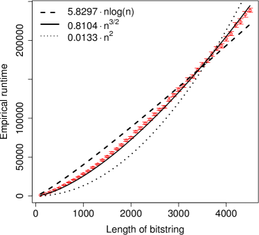
(a) small $\mu$

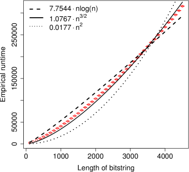
(b) large $\mu$

Figure 1: Mean runtime of the UMDA on OneMax with 95% confidence intervals plotted with error bars in red colour. Models are also fitted via non-linear regression.

We therefore experimented with two different settings for the parent population size: $\mu=\sqrt{n}$ and $\mu=\sqrt{n}\log(n)$. We call the first setting small population and the other large population. The empirical runtimes are shown in Figure 1. Theorem 1 implies the upper bounds $\mathcal{O}(n^{2})$ for the setting of small population and $\mathcal{O}(n^{3/2})$ for the setting of large population. Following bib:Lehre2014 , we identify the three positive constants $c_{1},c_{2}$ and $c_{3}$ that best fit the models $c_{1}n\log n$, $c_{2}n^{3/2}$ and $c_{3}n^{2}$ in non-linear least square regression. Note in particular that these models were chosen because they are close to the theoretical results. The correlation coefficient $\rho$ is then calculated for each model to find the best-fit model.

Table 2: Correlation coefficient $\rho$ for the best-fit models in the experiments with OneMax shown in Figures 1a and 1b.

Setting	Model	$\boldsymbol{\rho}$
$\mu=\sqrt{n}$	$5.8297\;n\log n$	$0.9968$
	$0.8104\;n^{3/2}$	$\mathbf{0.9996}$
	$0.0133\;n^{2}$	$0.9910$
$\mu=\sqrt{n}\log n$	$7.7544\;n\log n$	$0.9974$
	$1.0767\;n^{3/2}$	$\mathbf{0.9995}$
	$0.0177\;n^{2}$	$0.9903$

In Table 2, we observe that for small parent populations (i.e. $\mu=\sqrt{n}$), model $0.8104\;n^{3/2}$ fits the empirical data best, while the quadratic model gives the worst result. For larger parent population (i.e. $\mu=\sqrt{n}\log n$), the model $1.0767~{}n^{3/2}$ fits best the empirical data among the three models. Since $0.8104~{}n^{3/2}\in\mathcal{O}(n^{2})$, these findings are consistent with the theoretical expected optimisation time and may further suggest that the quadratic bound in case of small population is not tight.

5.2 LeadingOnes

We conducted experiments with $\mu=\sqrt{n}$, and $\lambda=n$. According to Theorem 1, the upper bound of the expected runtime is in this case $\mathcal{O}(n\lambda\log\lambda+n^{2})=\mathcal{O}(n^{2}\log n)$. Figure 2 shows the empirical runtime. Similarly to the OneMax problem, we fit the empirical runtime with four different models – $c_{1}n\log n$, $c_{2}n^{3/2}$, $c_{3}n^{2}$ and $c_{4}n^{2}\log n$ – using non-linear regression. The best values of the four constants are shown in Table 3 along with the correlation coefficients of the models.

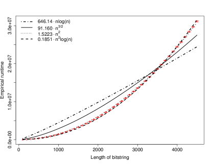
Figure 2: Mean runtime of the UMDA on LeadingOnes with 95% confidence intervals plotted with error bars in red colour. Models are also fitted via non-linear regression.

Table 3: Correlation coefficient $\rho$ for the best-fit models in the experiments with LeadingOnes shown in Figure 2.

Setting	Model	$\boldsymbol{\rho}$
$\mu=\sqrt{n}$	$646.14\;n\log n$	$0.9756$
	$91.160\;n^{3/2}$	$0.9928$
	$1.5223\;n^{2}$	$\mathbf{0.9999}$
	$0.1851\;n^{2}\log n$	$\mathbf{0.9999}$

Figure 2 and Table 3 show that both the model $1.5223~{}n^{2}$ and the model $0.1851~{}n^{2}\log n$, having the same correlation coefficient, fit well with the empirical data (i. e. the empirical data lie between these two curves). This finding is consistent with the theoretical runtime bound $\mathcal{O}(n^{2}\log n)$. Note also that these two models differ asymptotically by $\Theta(\log n)$, suggesting that our analysis of the UMDA on LeadingOnes is nearly tight.

5.3 BinVal

Finally, we consider BinVal. The upper bound $\mathcal{O}(n\lambda\log\lambda+n^{2})$ from Theorem 1 for the function is identical to the bound for LeadingOnes. Since BinVal is also a linear function like OneMax, we decided to set the experiments similarly for these functions, i. e. with different parent populations $\mu=\sqrt{n}$ and $\mu=\sqrt{n}\log n$. The empirical results are shown in Figure 3. Again the empirical runtime is fitted to the three models $c_{1}n\log n$, $c_{2}n^{3/2}$ and $c_{3}n^{2}$. The best values of $c_{1},c_{2}$ and $c_{3}$ are listed in Table 4, along with the correlation coefficient for each model.

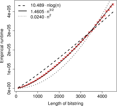
(a) small $\mu$

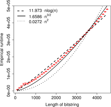
(b) large $\mu$

Figure 3: Mean runtime of the UMDA on BinVal with 95% confidence intervals plotted with error bars in red colour. Models are also fitted via non-linear regression.

Table 4: Correlation coefficient $\rho$ for the best-fit models in the experiments with BinVal shown in Figures 3a and 3b

Setting	Model	$\boldsymbol{\rho}$
$\mu=\sqrt{n}$	$10.489\;n\log n$	$0.9952$
	$1.4605\;n^{3/2}$	$\mathbf{0.9999}$
	$0.0240\;n^{2}$	$0.9933$
$\mu=\sqrt{n}\log n$	$11.973\;n\log n$	$0.9972$
	$1.6596\;n^{3/2}$	$\mathbf{0.9994}$
	$0.0272\;n^{2}$	$0.9903$

Theorem 1 gives the upper bound of $\mathcal{O}(n^{2}\log n)$ for the expected runtime of BinVal. However, Figure 3 and Table 4 show clearly that the model $1.4605\;n^{3/2}$ fits best the empirical runtime for $\mu=\sqrt{n}$. On the other hand, the empirical runtime lies between the two models $11.973\;n\log n$ and $1.6586\;n^{3/2}$ when $\mu=\sqrt{n}\log n$. While these observations are consistent with the theoretical upper bound since $\mathcal{O}(n^{3/2})$ and $\mathcal{O}(n\log n)$ are all members of $\mathcal{O}(n^{2}\log n)$, they also suggest that our analysis of the UMDA on BinVal given by Theorem 1 may be loose.

6 Conclusion

Despite the popularity of EDAs in real-world applications, little has been known about their theoretical optimisation time, even for apparently simple settings such as the UMDA on toy functions. More results for the UMDA on these simple problems with well-understood structures provide a way to describe and compare the performance of the algorithms with other search heuristics. Furthermore, results about the UMDA are not only relevant to evolutionary computation, but also to population genetics where it corresponds to the notion of linkage equilibrium bib:muhlenbein2002 ; bib:Slatkin2008 .

We have analysed the expected optimisation time of the the UMDA on three benchmark problems: OneMax, LeadingOnes and BinVal. For both LeadingOnes and BinVal, we proved the upper bound of $\mathcal{O}(n\lambda\log\lambda+n^{2})$, which holds for $\lambda=\Omega(\log n)$. For OneMax, two upper bounds of $\mathcal{O}(\lambda n)$ and $\mathcal{O}(\lambda\sqrt{n})$ were obtained for $\mu=\Omega(\log n)\cap\mathcal{O}(\sqrt{n})$ and $\mu=\Omega(\sqrt{n}\log n)$, respectively. Although our result assumes that $\lambda\geq(1+\beta)\mu$ for some positive constant $\beta>0$, it no longer requires that $\lambda=\Theta(\mu)$ as in bib:Witt2017 . Note that if $\lambda=\Theta(\log n)$, a tight bound of $\Theta(n\log n)$ on the expected optimisation time of the UMDA on OneMax is obtained, matching the well-known tight bound of $\Theta(n\log n)$ for the (1+1) EA on the class of linear functions. Although we did not obtain a runtime bound when the parent population size is $\mu=\Omega(\sqrt{n})\cap\mathcal{O}(\sqrt{n}\log n)$, our results finally close the existing $\Theta(\log\log n)$-gap between the first upper bound of $\mathcal{O}(n\log n\log\log n)$ for $\lambda=\Omega(\mu)$ bib:Dang2015a and the relatively new lower bound of $\Omega(\mu\sqrt{n}+n\log n)$ for $\lambda=(1+\Theta(1))\mu$ bib:Krejca .

Our analysis further demonstrates that the level-based theorem can yield, relatively easily, asymptotically tight upper bounds for non-trivial, population-based algorithms. An important additional component of the analysis was the use of anti-concentration properties of the Poisson-Binomial distribution. Unless the variance of the sampled individuals is not too small, the distribution of the population cannot be too concentrated anywhere, even around the mean, yielding sufficient diversity to discover better solutions. We expect that similar arguments will lead to new results in runtime analysis of evolutionary algorithms.

Appendix A Appendix

Lemma 1 (mitrinovic1970analytic ).

For all $t\in\mathbb{R}$ and $n\in\mathbb{R}^{+}$,

$$\left(1+\frac{t}{n}\right)^{n}\leq e^{t}\leq\left(1+\frac{t}{n}\right)^{n+t/2}.$$

Lemma 2 (Theorem 3.2, bib:Jogdeo ).

Let $Y_{1},Y_{2},\ldots,Y_{n}$ be $n$ independent Bernoulli random variables, and $Y\coloneqq\sum_{i=1}^{n}Y_{i}$ is the sum of these random variables. If $\mathbb{E}[Y]$ is an integer, then

$$\Pr\left(Y\geq\mathbb{E}[Y]\right)\geq 1/2.$$

Lemma 3 (Stirling’s approximation bib:LCRC ).

For all $n\in\mathbb{N}$,

$$n!=\Theta\left(\frac{n^{n+1/2}}{e^{n}}\right).$$

In the following we write $X\preceq Y$ to denote that random variable $Y$ stochastically dominates random variable $X$, i. e. $\Pr\left(X\geq k\right)\leq\Pr\left(Y\geq k\right)$ for all $k\in\mathbb{R}$. The lemma below can be easily proved with coupling argument bib:Roch2015 .

Lemma 4.

Let $X_{1},X_{2},Y_{1}$ and $Y_{2}$ be independent random variables such that $X_{1}\succeq Y_{1}$ and $X_{2}\succeq Y_{2}$. Then $X_{1}+X_{2}\succeq Y_{1}+Y_{2}$.

Proof.

The proof is taken from Corollary 4.27 in bib:Roch2015 . Let $(\hat{X}_{1},\hat{Y}_{1})$ and $(\hat{X}_{2},\hat{Y}_{2})$ be independent, monotone couplings of $(X_{1},Y_{1})$ and $(X_{2},Y_{2})$ on the same probability space. It then holds that $X_{1}+X_{2}\sim\hat{X}_{1}+\hat{X}_{2}\succeq\hat{Y}_{1}+\hat{Y}_{2}\sim Y_{1}+Y_{2}$. ∎

Lemma 5 (Lemma 3, bib:Wu2017 ).

Let $Y_{1},\ldots,Y_{n}$ be $n$ independent Bernoulli random variables with success probabilities $p_{1},\ldots,p_{n}$. Let $Y:=\sum_{i=1}^{n}Y_{i}$ be the sum of these variables. If $p_{i}\geq p_{\min}$ for all $i\in[n]$, where $p_{\min}>0$ is a constant, and any constant $d^{*}\geq 1/p_{\min}$ then

$$\Pr\left(Y\geq\min\bigg{\{}\mathbb{E}\left[Y\right]+d^{*}\sqrt{n-\lfloor\mathbb{E}[Y]\rfloor},n\bigg{\}}\right)\geq\kappa,$$

where $\kappa$ is a positive constant independent of $n$.

Lemma 6.

For any $n\in\mathbb{N}$, any constant $d\in(0,1]$ independent to $n$ and the sequence $(f_{i})_{i\in\mathbb{N}}$ defined according to (11), it holds that

(i)

$f_{i}\leq n$ for all $i\in\mathbb{N}$, and $\exists j\in\mathbb{N}\colon f_{j}=n$,

(ii)

if $\ell=\min\{i\in\mathbb{N}\mid f_{i}=n\}$ then $\ell=\Theta(\sqrt{n})$.

Proof.

We first prove (i), it is easy to see that $f_{i}$ are all integer, i. e. $f_{i}\in\mathbb{N}$ for all $i\in\mathbb{N}$. Due to the ceiling function if $f_{i}<n$, then $f_{i+1}\geq f_{i}+1$, in other words starting with $f_{0}=0$, the sequence will increase steadily until it hits $n$ exactly or overshoots it. Assuming the later case of overshooting, that is, $\exists k\geq 0\colon f_{k}\leq n-1$ and $f_{k+1}\geq n+1$ (and after that $f_{k+2},\dots$ are ill-defined). By the definition of the sequence, the property $1+x>\lceil x\rceil$ of the ceiling function and $d\leq 1$, we have

$$1+\sqrt{n-f_{k}}>\lceil\sqrt{n-f_{k}}\rceil\geq\lceil d\sqrt{n-f_{k}}\rceil=f_{k+1}-f_{k}\geq 2,$$

this implies $f_{k}<n-1$ or $f_{k}\leq n-2$. Repeating the above argument again gives that $1+\sqrt{n-f_{k}}>3$, and $f_{k}<n-4$, after a finite number of repetitions we will conclude that $f_{k}<0$ which is a contradiction. Therefore, the sequence must hit $n$ exactly at one point in time then it will remain at that value.

To bound $\ell$ in (ii), we pair $(f_{i})_{i\in\mathbb{N}}$ with $(r_{i}:=\sqrt{n-f_{i}})_{i\in\mathbb{N}}$; thus, this sequence starts at $r_{0}=\sqrt{n}$, then decreases and eventually hits $0$, that is, $\sqrt{n}=r_{0}>r_{1}>r_{2}>\dots>r_{\ell-1}>r_{\ell}=0$. From (11), we have

$$(r_{i}-r_{i+1})(r_{i}+r_{i+1}) =r_{i}^{2}-r_{i+1}^{2}=f_{i+1}-f_{i}=\lceil dr_{i}\rceil,$$

note that $1+dr_{i}>\lceil dr_{i}\rceil\geq dr_{i}$, then for $i\leq\ell-1$, we can divide both sides by $r_{i}+r_{i+1}>0$ to get

$$\frac{1+dr_{i}}{r_{i}+r_{i+1}}>r_{i}-r_{i+1}\geq\frac{dr_{i}}{r_{i}+r_{i+1}}.$$

Always restricted to $i\leq\ell-1$, we have that $1>r_{i+1}/r_{i}\geq 0$, and therefore $dr_{i}/(r_{i}+r_{i+1})=d/(1+r_{i+1}/r_{i})>d/2$. In addition, $f_{i}\leq n-1$ then $r_{i}=\sqrt{n-f_{i}}\geq 1$ or $1/r_{i}\leq 1$, so $(1+dr_{i})/(r_{i}+r_{i+1})=(1/r_{i}+d)/(1+r_{i+1}/r_{i})\leq d+1$. Therefore, for all $i\leq\ell-1$

$$d+1>r_{i}-r_{i+1}>\frac{d}{2}.$$

Summing all these terms gives that

$$\ell(d+1)>\sum_{i=0}^{\ell-1}(r_{i}-r_{i+1})=r_{0}-r_{\ell}=\sqrt{n}>\frac{\ell d}{2},$$

and this implies $2\sqrt{n}/d>\ell>\sqrt{n}/(d+1)$, or $\ell=\Theta(\sqrt{n})$. ∎

Lemma 7.

Let $Y_{1},Y_{2},\ldots,Y_{k}$ be $k$ ($k\geq 1$) independent Bernoulli random variables with success probabilities $p_{1},p_{2},\ldots,p_{k}$, where $p_{i}\geq p_{\min}=1/4$ for each $i\in[k]$. Let $Y_{1,k}:=\sum_{i=1}^{k}Y_{i}$. Then we always have

$$\Pr\left(Y_{1,k}\geq\mathbb{E}\left[Y_{1,k}\right]\right)\geq\Omega(1).$$

Proof.

We start by considering small values of $k$. If $k=1$, then

$$\Pr\left(Y_{1,1}\geq\mathbb{E}\left[Y_{1,1}\right]\right)=\Pr(Y_{1}=1)=p_{1}\geq 1/4.$$

If $k=2$, then

$$\Pr\left(Y_{1,2}\geq\mathbb{E}[Y_{1,2}]\right)\geq\Pr\left(Y_{1}=1\right)\cdot\Pr\left(Y_{2}=1\right)\geq p_{1}p_{2}\geq(1/4)^{2}.$$

For larger values of $k$, following bib:Wu2017 we introduce another random variable $Z=\left(Z_{1},\ldots,Z_{k}\right)$ with success probabilities $z_{1},\ldots,z_{k}$, where $z_{i}\geq p_{\min}$ and $\mathbb{E}[Z_{1,k}]=\sum_{i=1}^{k}z_{i}=\sum_{i=1}^{k}p_{i}=\mathbb{E}\left[Y_{1,k}\right]$. However, we shift the total weight $\mathbb{E}\left[Y_{1,k}\right]$ as far as possible to the $Z_{i}$ with smaller indices as follows. We define $m=\lfloor\frac{\mathbb{E}[Y_{1,k}]-kp_{\min}}{1-p_{\min}}\rfloor$, and let $Z_{1},\ldots,Z_{m}$ all get success probability 1, and $Z_{m+2},\ldots,Z_{k}$ get $z_{i}=p_{\min}$, more precisely

$$z_{i}=\begin{cases}~{}1,&\text{for }i=1,\ldots,m,\\ ~{}q,&\text{for }i=m+1,\\ ~{}p_{\min},&\text{for }i=m+2,\ldots,k,\end{cases}$$

where $q\in[p_{\min},1]$. It is quite clear that $(z_{1},\ldots,z_{k})$ majorises $\left(p_{t}(1),\ldots,p_{t}(k)\right)$. From marshall1979inequalities ; gleser1975 , we now have

$$\Pr\left(Y_{1,k}\geq\mathbb{E}\left[Y_{1,k}\right]\right) \geq\Pr\left(Y_{1,k}\geq\mathbb{E}\left[Y_{1,k}\right]+1\right)$$

$$\geq\Pr(Z_{1,k}\geq\mathbb{E}\left[Z_{1,k}\right]+1).$$

Furthermore, with probability $1$ we can get $m$ ones and

$$\mathbb{E}[Z_{m+2,k}]=\mathbb{E}\left[Z_{1,k}\right]-m-q\iff\mathbb{E}[Z_{m+2,k}]+q=\mathbb{E}\left[Z_{1,k}\right]-m,$$

then

$$\Pr(Z_{1,k} \geq\mathbb{E}\left[Z_{1,k}\right]+1)$$

$$\geq\Pr(Z_{m+1,k}\geq\mathbb{E}\left[Z_{1,k}\right]+1-m)$$

$$\geq\Pr(Z_{m+1}=1)\cdot\Pr(Z_{m+2,k}\geq\mathbb{E}\left[Z_{1,k}\right]-m)$$

$$=q\cdot\Pr(Z_{m+2,k}\geq\mathbb{E}[Z_{m+2,k}]+q)$$

$$\geq p_{\min}\cdot\Pr(Z_{m+2,k}\geq\mathbb{E}[Z_{m+2,k}]+1).$$

The last inequality follows the fact that $p_{\min}\leq q\leq 1$. We now need a lower bound on the probability $\Pr(Z_{m+2,k}\geq\mathbb{E}[Z_{m+2,k}]+1)$, where

$$Z_{m+2,k}\sim\text{Bin}\left(k-m-1,\frac{1}{4}\right).$$

Now let $k-m-1=4t+x=4(t-1)+x+4$, where $t\in\mathbb{N}$ and $x\in\{0,1,2,3\}$. Then $\mathbb{E}[Z_{m+2,k}]=t+\frac{x}{4}$, and

$$\Pr(Z_{m+2,k}\geq\mathbb{E}[Z_{m+2,k}]+1)$$

$$=\Pr(Z_{m+2,k}\geq t+\frac{x}{4}+1)$$

$$\geq\Pr\left(Z_{m+2,k}\geq 4(t-1)+x+4\right)$$

$$\geq\Pr(Z_{m+2,m+2+4(t-1)-1}\geq t-1)$$

$$\qquad\qquad\cdot\Pr(Z_{m+2+4(t-1),n}\geq x+4)$$

$$=\Pr(Z_{m+2,m+2+4(t-1)-1}\geq\mathbb{E}[Z_{m+2,m+2+4(t-1)-1}])$$

$$\qquad\qquad\cdot\Pr(Z_{m+2+4(t-1),n}\geq x+4)$$

$$\geq\frac{1}{2}\cdot\left(\frac{1}{4}\right)^{x+4}\geq\frac{1}{2}\cdot\left(\frac{1}{4}\right)^{7}.$$

The result follows Lemma 2, where $\mathbb{E}[Z_{m+2,m+2+4(t-1)-1}]$ is an integer, and $x\leq 3$. ∎

Lemma 8.

For any constant $d\leq 1$ and $\mathbb{E}[Y_{1,n}]\geq f_{j-1}-\ell/n$, it holds that

$$\mathbb{E}\left[Y_{1,n}\right]+d\sqrt{n-\mathbb{E}\left[Y_{1,n}\right]}\geq f_{j-1}+d\sqrt{n-f_{j-1}}.$$ (15)

Proof.

Let us rewrite (14) by introducing a variable $x\geq 0$ as follows:

$$\mathbb{E}\left[Y_{1,n}\right]=f_{j-1}-\frac{\ell}{n}+x$$ (16)

We consider two different cases.

• Case 1: If $x=\ell/n$, then $\mathbb{E}\left[Y_{1,n}\right]=f_{j-1}$, and the lemma holds for all values of $d$.

• Case 2: If $x\neq\ell/n$, then substituting (16) into (15) and let $y:=x-\ell/n\in[-\ell/n,0)\cup(0,n-f_{j-1}]$, we have

  $$d\leq g\left(y,f_{j-1}\right):=\frac{y}{\sqrt{n-f_{j-1}}-\sqrt{n-f_{j-1}-y}}$$

  This always holds if we pick a constant

  $$d\leq\min_{y,f_{j-1}}g\left(y,f_{j-1}\right).$$

  From $\partial g/\partial y=0$, we obtain $y=0$. Note that when $y=0$, $\partial^{2}g/\partial y^{2}<0$. This means $g(y,f_{j-1})$ reaches the maximum value when $y=0$ with respect to $f_{j-1}$, and

  $$g\left(y,f_{j-1}\right)$$

  $$\geq\min\big{\{}g\left(-\ell/n,f_{j-1}\right),g\left(n-f_{j-1},f_{j-1}\right)\big{\}}$$

  $$=\min\big{\{}\sqrt{n-f_{j-1}},\sqrt{n-f_{j-1}}+\sqrt{n-f_{j-1}+\ell/n}\big{\}}$$

  $$=\sqrt{n-f_{j-1}}$$

  $$\geq\min_{f_{j-1}}\big{\{}\sqrt{n-f_{j-1}}\big{\}}$$

  $$=1$$

  due to $f_{j-1}\leq n-1$.

The lemma is proved by combining results of the two cases. ∎

References

- [1] Rubén Armañanzas, Iñaki Inza, Roberto Santana, Yvan Saeys, Jose Luis Flores, Jose Antonio Lozano, Yves Van de Peer, Rosa Blanco, Víctor Robles, Concha Bielza, and Pedro Larrañaga. A review of estimation of distribution algorithms in bioinformatics. BioData Mining, 1(1):6, 2008.
- [2] Hideki Asoh and Heinz Mühlenbein. On the mean convergence time of evolutionary algorithms without selection and mutation. In Proceedings of the 3rd International Conference on Parallel Problem Solving from Nature, PPSN III, pages 88–97, 1994.
- [3] Jean-Bernard Baillon, Roberto Cominetti, and José Vaisman. A sharp uniform bound for the distribution of sums of bernoulli trials. Combinatorics, Probability and Computing, 25(3):352–361, 2016.
- [4] Shummet Baluja. Population-based incremental learning: A method for integrating genetic search based function optimization and competitive learning. Technical report, Carnegie Mellon University, 1994.
- [5] Tianshi Chen, Per Kristian Lehre, Ke Tang, and Xin Yao. When is an estimation of distribution algorithm better than an evolutionary algorithm? In Proceedings of 2009 IEEE Congress on Evolutionary Computation, pages 1470–1477, 2009.
- [6] Tianshi Chen, Ke Tang, Guoliang Chen, and Xin Yao. On the analysis of average time complexity of estimation of distribution algorithms. In Proceedings of 2007 IEEE Congress on Evolutionary Computation, pages 453–460, 2007.
- [7] Tianshi Chen, Ke Tang, Guoliang Chen, and Xin Yao. Rigorous time complexity analysis of univariate marginal distribution algorithm with margins. In Proceedings of 2009 IEEE Congress on Evolutionary Computation, pages 2157–2164, 2009.
- [8] Tianshi Chen, Ke Tang, Guoliang Chen, and Xin Yao. Analysis of computational time of simple estimation of distribution algorithms. IEEE Transactions on Evolutionary Computation, 14(1):1–22, 2010.
- [9] Dogan Corus, Duc-Cuong Dang, Anton V. Eremeev, and Per Kristian Lehre. Level-based analysis of genetic algorithms and other search processes. IEEE Transactions on Evolutionary Computation, pages 1–1, 2017.
- [10] Duc-Cuong Dang and Per Kristian Lehre. Simplified runtime analysis of estimation of distribution algorithms. In Proceedings of Genetic and Evolutionary Computation, GECCO’15, pages 513–518, 2015.
- [11] Duc-Cuong Dang and Per Kristian Lehre. Self-adaptation of mutation rates in non-elitist populations. In Proceedings of the 14th International Conference on Parallel Problem Solving from Nature, PPSN XIV, pages 803–813, 2016.
- [12] Benjamin Doerr and Martin S. Krejca. Significance-based estimation-of-distribution algorithms. In Proceedings of Genetic and Evolutionary Computation Conference, GECCO’18, pages 1483–1490, 2018.
- [13] Stefan Droste. A rigorous analysis of the compact genetic algorithm for linear functions. Natural Computing, 5(3):257–283, 2006.
- [14] Els I. Ducheyne, Bernard De Baets, and Robert R. De Wulf. Probabilistic Models for Linkage Learning in Forest Management, pages 177–194. Springer Berlin Heidelberg, 2005.
- [15] Uriel Feige. On sums of independent random variables with unbounded variance and estimating the average degree in a graph. SIAM Journal on Computing, 35(4):964–984, 2006.
- [16] Tobias Friedrich, Timo Kötzing, Martin Krejca, and Andrew M. Sutton. The compact genetic algorithm is efficient under extreme gaussian noise. IEEE Transactions on Evolutionary Computation, 21(3):477–490, 2017.
- [17] Tobias Friedrich, Timo Kötzing, and Martin S. Krejca. EDAs cannot be balanced and stable. In Proceedings of Genetic and Evolutionary Computation Conference, GECCO’16, pages 1139–1146, 2016.
- [18] Leon Jay Gleser. On the distribution of the number of successes in independent trials. The Annals of Probability, 3(1):182–188, 1975.
- [19] Wei Gu, Yonggang Wu, and GuoYong Zhang. A hybrid univariate marginal distribution algorithm for dynamic economic dispatch of units considering valve-point effects and ramp rates. International Transactions on Electrical Energy Systems, 25(2):374–392, 2015.
- [20] Georges R. Harik, Fernando G. Lobo, and David E. Goldberg. The compact genetic algorithm. IEEE Transactions on Evolutionary Computation, 3(4):287–297, 1999.
- [21] Mark Hauschild and Martin Pelikan. An introduction and survey of estimation of distribution algorithms. Swarm and Evolutionary Computation, 1(3):111–128, 2011.
- [22] Kumar Jogdeo and Stephen M. Samuels. Monotone convergence of binomial probabilities and a generalization of ramanujan‘s equation. The Annals of Mathematical Statistics, 39(4):1191–1195, 1968.
- [23] Joshua B. Kollat, Patrick M. Reed, and Joseph R. Kasprzyk. A new epsilon-dominance hierarchical bayesian optimization algorithm for large multiobjective monitoring network design problems. Advances in Water Resources, 31(5):828–845, 2008.
- [24] Martin S. Krejca and Carsten Witt. Theory of estimation-of-distribution algorithms. In Benjamin Doerr and Frank Neumann, editors, Theory of Randomized Search Heuristics in Discrete Search Spaces. Springer. to appear.
- [25] Martin S. Krejca and Carsten Witt. Lower bounds on the run time of the univariate marginal distribution algorithm on onemax. In Proceedings of Foundations of Genetic Algorithms XIV, FOGA’17, pages 65–79, 2017.
- [26] Per Kristian Lehre and Phan Trung Hai Nguyen. Improved runtime bounds for the univariate marginal distribution algorithm via anti-concentration. In Proceedings of Genetic and Evolutionary Computation Conference, GECCO’17, pages 1383–1390, 2017.
- [27] Per Kristian Lehre and Phan Trung Hai Nguyen. Level-based analysis of the population-based incremental learning algorithm. In Proceedings of the 15th International Conference on Parallel Problem Solving from Nature, PPSN XV, 2018. to appear.
- [28] Per Kristian Lehre and Carsten Witt. Black-box search by unbiased variation. In Proceedings of Genetic and Evolutionary Computation Conference, GECCO’10, pages 1441–1448, 2010.
- [29] Per Kristian Lehre and Xin Yao. Runtime analysis of the (1+1) EA on computing unique input output sequences. Information Sciences, 259:510–531, 2014.
- [30] Charles E. Leiserson, Clifford Stein, Ronald Rivest, and Thomas H. Cormen. Introduction to Algorithms. MIT Press, 2009.
- [31] Johannes Lengler, Dirk Sudholt, and Carsten Witt. Medium step sizes are harmful for the compact genetic algorithm. In Proceedings of Genetic and Evolutionary Computation Conference, GECCO’18, pages 1499–1506, 2018.
- [32] Albert W Marshall, Ingram Olkin, and Barry C Arnold. Inequalities: Theory of Majorization and Its Applications. Springer-Verlag New York, 2011.
- [33] Pascal Massart. The tight constant in the Dvoretzky-Kiefer-Wolfowitz inequality. The Annals of Probability, 18(3):1269–1283, 1990.
- [34] Dragoslav S. Mitrinovic. Analytic Inequalities. Springer Berlin Heidelberg, 1970.
- [35] Heinz Mühlenbein and Thilo Mahnig. Evolutionary computation and wright‘s equation. Theoretical Computer Science, 287:145–165, 2002.
- [36] Heinz Mühlenbein and Gerhard Paaß. From recombination of genes to the estimation of distributions i. binary parameters. In Proceedings of the 9th International Conference on Parallel Problem Solving from Nature, PPSN IV, pages 178–187, 1996.
- [37] Sebastien Roch. Modern Discrete Probability: An Essential Toolkit. Book in preparation, 2015.
- [38] Reuven Y. Rubinstein and Dirk P. Kroese. The Cross Entropy Method: A Unified Approach To Combinatorial Optimization, Monte-carlo Simulation (Information Science and Statistics). Springer-Verlag New York, 2004.
- [39] Roberto Santana, Alexander Mendiburu, and Jose A. Lozano. A review of message passing algorithms in estimation of distribution algorithms. Natural Computing, 15(1):165–180, 2016.
- [40] Jonathan L. Shapiro. Drift and scaling in estimation of distribution algorithms. Evolutionary Computation, 13(1):99–123, 2005.
- [41] Montgomery Slatkin. Linkage disequilibrium — understanding the evolutionary past and mapping the medical future. Nature Reviews Genetics, 9(6):477–485, 2008.
- [42] Dirk Sudholt and Carsten Witt. Update strength in EDAs and ACO: How to avoid genetic drift. In Proceedings of Genetic and Evolutionary Computation Conference, GECCO’16, pages 61–68, 2016.
- [43] Bartel Leendert van der Waerden. Algebra, volume 1. Springer-Verlag New York, 1991.
- [44] Carsten Witt. Upper bounds on the runtime of the univariate marginal distribution algorithm on onemax. In Proceedings of Genetic and Evolutionary Computation Conference, GECCO’17, pages 1415–1422, 2017.
- [45] Carsten Witt. Domino convergence: why one should hill-climb on linear functions. In Proceedings of Genetic and Evolutionary Computation Conference, GECCO’18, pages 1539–1546, 2018.
- [46] Zijun Wu, Michael Kolonko, and Rolf H. Möhring. Stochastic runtime analysis of the cross-entropy algorithm. IEEE Transactions on Evolutionary Computation, 21(4):616–628, 2017.
- [47] Tian-Li Yu, Scott Santarelli, and David E. Goldberg. Military Antenna Design Using a Simple Genetic Algorithm and hBOA, pages 275–289. Springer Berlin Heidelberg, 2006.
- [48] Lyudmila Zinchenko, Heinz Mühlenbein, Viktor Kureichik, and Thilo Mahnig. Application of the univariate marginal distribution algorithm to analog circuit design. In Proceedings of 2002 NASA/DoD Conference on Evolvable Hardware, pages 93–101, 2002.