Modeling the Milky Way as a Dry Galaxy

Abstract

We construct a model for the Milky Way Galaxy composed of a stellar disc and bulge embedded in a dark-matter halo. All components are modelled as $N$-body systems with up to 8 billion equal-mass particles and integrated up to an age of 10 Gyr. We find that net angular-momentum of the dark-matter halo with a spin parameter of $\lambda=0.06$ is required to form a relatively short bar ($\sim 4$ kpc) with a high pattern speed (40–50 km s^-1). By comparing our model with observations of the Milky Way Galaxy, we conclude that a disc mass of $\sim 3.7\times 10^{10}M_{\odot}$ and an initial bulge scale length and velocity of $\sim 1$ kpc and $\sim 300$ km s^-1, respectively, fit best to the observations. The disc-to-total mass fraction ($f_{\rm d}$) appears to be an important parameter for the evolution of the Galaxy and models with $f_{\rm d}\sim 0.45$ are most similar to the Milky Way Galaxy. In addition, we compare the velocity distribution in the solar neighbourhood in our simulations with observations in the Milky Way Galaxy. In our simulations the observed gap in the velocity distribution, which is expected to be caused by the outer Lindblad resonance (the so-called Hercules stream), appears to be a time-dependent structure. The velocity distribution changes on a time scale of 20–30 Myr and therefore it is difficult to estimate the pattern speed of the bar from the shape of the local velocity distribution alone.

1 Introduction

Simulating the Milky Way (MW) Galaxy as an $N$-body system without gas is an important step in understanding its structure, kinematics, and dynamics. The complex structures of the Galactic disc such as the bar and spiral structures are composed of a bunch of individual stars orbiting around the Galactic center. We can examine the self-consistent evolution of the disc, bulge, and halo using $N$-body simulations. Especially when using models in which the dark-matter halo is composed of particles as opposed to an analytic potential, we are able to follow the evolution of the bar as it emits the discs angular momentum to the live halo (Athanassoula, 2002; Dubinski et al., 2009).

Self-consistent MW models with a ‘live’ dark-matter halo have been proposed by several previous studies (Widrow & Dubinski, 2005; Fux, 1997). Widrow & Dubinski (2005) proposed a self-consistent equilibrium model of the MW. They constructed the distribution functions of the disc with a bulge and halo from integrals of motions by iteratively solving the Poisson equation (Kuijken & Dubinski, 1995). The resulting model is compared with observational properties such as the rotation curve and the line-of-sight velocity-dispersion profile of the bulge region (Tremaine et al., 2002). They proposed two models for the MW; one disc-dominated model and one halo-dominated model, both of which with a relatively massive bulge ($M_{\rm b}>10^{10}M_{\odot}$). In Shen et al. (2010) the authors found, using $N$-body simulations, that a model with a small bulge (less than $\sim 8$ % of the disc mass) fits the bulge kinematics data, observed by the Bulge Radial Velocity Assay (BRAVA) (Howard et al., 2008; Kunder et al., 2012), better than the previously predicted massive classical bulge. Apart from the bulge kinematics, there is additional available observational data of the MW such as the velocity dispersion of the disc stars and surface density of the disc measured in the solar neighbourhood (Bland-Hawthorn & Gerhard, 2016).

Here we construct an improved self-gravitating model for the MW that takes these observations into account. We perform a range of $N$-body simulations using models that are setup using the methods described in Kuijken & Dubinski (1995) and Widrow & Dubinski (2005) (see § 2).

One of the difficulties in finding the initial conditions for a best fitting Galaxy model is that we cannot predict the outcome of the simulation before actually having performed the run. The chaotic gravitational dynamics of the particles (see Portegies Zwart & Boekholt (2018) for a brief overview) prevents making a preliminary assessment of the simulation results as function of the many initial parameters. Although many automated optimization strategies exist, we decided to do this by manually mapping the parameter space and guiding our next run based on the analyzed data. This is a rather labour intensive procedure, but allows us to converge more efficiently than any automated procedure.

We perform the simulations with at least one million particles in the Galactic disc. Such a large number of particles is necessary in order to obtain a reliable result at the end of the simulation (Fujii et al., 2011). To simulate our models we use our recently developed tree-code, Bonsai, which utilizes massive parallel GPU computing systems (Bédorf et al., 2014). Using Bonsai, we are able to perform a large number of $N$-body simulations, with a high enough resolution. Our largest model contains eight billion particles for the galaxy and the dark-matter halo combined. By comparing the properties of the simulated model with recent MW observations, we find the best matching configuration parameters.

We further “observe” the largest simulations in order to compare the results with the MW Galaxy to investigate the velocity distribution in the local neighbourhood. It is expected that spiral structures can be seen in the local velocity distribution as well as the imprint of resonances such as the Hercules stream, although the origin of the velocity structures is still debatable (Dehnen, 2000; Quillen et al., 2011; Antoja et al., 2014; Monari et al., 2017; Pérez-Villegas et al., 2017; Hunt et al., 2018b; Hunt & Bovy, 2018; Hattori et al., 2018). In this paper, we propose a set of best matching parameters for the MW Galaxy and make a comparison with observations. In Section 2, we describe the details of our models and $N$-body simulations. Our best-fitting models are presented in Section 3. In Section 4, we show detailed analyses of the best-fitting models. The results are summarized in Section 5.

2 $N$-body simulations

To find a best-fitting MW model we performed a series of $N$-body simulations. We simulate a live dark-matter halo with an embedded stellar disc. The simulations have up to $\sim 8$ billion particles.

The initial conditions are generated using GalactICSand the simulations are performed using the parallel GPU tree-code, Bonsai (Bédorf et al., 2012; Bédorf et al., 2014), which is part of the Astrophysical Multipurpose Software Environment (AMUSE, Portegies Zwart et al., 2013; Pelupessy et al., 2013; Portegies Zwart & McMillan, 2018). In this section details of the models, parameters, and simulations are described. Since we tested more than 50 models we only cover the most important models in the main text, the detailed parameters for all models are summarized in Appendix A.

2.1 Initial conditions

2.1.1 Dark-Matter Halo

In the initial condition generator, GalactICS (Kuijken & Dubinski, 1995; Widrow & Dubinski, 2005), the dark-matter halo is modeled using the NFW density profile (Navarro et al., 1997):

$$\rho_{\rm NFW}(r)=\frac{\rho_{\rm h}}{(r/a_{\rm h})(1+r/a_{\rm h})^{3}},$$ (1)

with the following potential:

$$\Phi_{\rm NFW}=-\sigma_{\rm h}^{2}\frac{\log(1+r/a_{\rm h})}{r/a_{\rm h}},$$ (2)

where $a_{\rm h}$ is the scale radius, $\rho_{\rm h}\equiv\sigma^{2}/(4{\rm\pi}Ga_{\rm h}^{2})$ is the characteristic density, and $\sigma_{\rm h}$ is the characteristic velocity dispersion. The gravitational constant, $G$, is set to be unity. Since the NFW profile has an infinite extent the mass distribution is truncated by a halo tidal radius using an energy cutoff $E_{\rm h}\equiv\epsilon_{\rm h}\sigma_{\rm h}^{2}$, where $\epsilon_{\rm h}$ is the truncation parameter with $0<\epsilon_{\rm h}<1$. Setting $\epsilon_{\rm h}=0$ yields a full NFW profile (see Widrow & Dubinski, 2005, for details).

We therefore have $a_{\rm h}$, $\sigma_{\rm h}$, $\epsilon_{\rm h}$, and $\alpha_{\rm h}$ as the parameters that configure the dark-matter halo model. We summarize the values of these parameters for our models in Tables 1 and 5. Here $a_{\rm h}$ and $\sigma_{\rm h}$ are chosen such that the models match the observed circular rotation velocity at the Sun’s location, $V_{\rm circ,\odot}=238\pm 15$ km s^-1 (Bland-Hawthorn & Gerhard, 2016). The Galactic virial radius is estimated to be $r_{\rm vir}=282\pm 30$ kpc (Bland-Hawthorn & Gerhard, 2016), and from cosmological simulations, we know that dark-matter halos with a mass of $10^{12}M_{\odot}$ typically have a concentration parameter of $c\equiv r_{\rm vir}/a_{\rm h}=10$–17 (Klypin et al., 2002). These give $a_{\rm h}\sim 15$–30 kpc. Recently it was suggested that $c\sim 10$ ($a_{\rm h}\sim 25$ kpc) (Correa et al., 2015), but theoretical modeling, based on observations, suggest smaller values such as $a_{\rm h}=19.0\pm 4.9$ kpc (McMillan, 2017) and $a_{\rm h}=14.39^{+1.30}_{-1.15}$ kpc (Huang et al., 2016). Our choice for $a_{\rm h}$ is on the lower end of the above ranges, namely 10–22 kpc.

To reproduce the observed circular rotational velocity at the location of the Sun, we set $\sigma_{\rm h}=380$–500 km s^-1. For $\epsilon_{\rm h}$, we use 0.7–0.85 to get an halo outer radius, $r_{\rm h}$, that is close to the observed Galactic virial radius, $r_{\rm vir}=282\pm 30$ kpc (Bland-Hawthorn & Gerhard, 2016). The above settings result in a halo mass, $M_{\rm h}$, of $\sim 6$–$19\times 10^{11}M_{\odot}$ (see Tables 2 and 6). In these tables we further see that the halo mass is most sensitive to the value of $a_{\rm h}$ if we fix the circular rotation velocity at the location of the Sun; if $a_{\rm h}$ is small then $M_{\rm h}$ is also small.

On the other hand, the MW’s virial mass is estimated to be $M_{\rm vir}=1.3\pm 0.3\times 10^{12}M_{\odot}$ (Bland-Hawthorn & Gerhard, 2016). In this work, we are interested in the halo’s inner region where the Galactic disc is located, because the outer region only has a limited effect on the disc evolution. We, therefore, consider the total halo mass and outer radius, which are configured using the truncation parameter ($\epsilon_{\rm h}$), of less significance in this work.

The final parameter that controls the halo configuration is the spin parameter $\alpha_{\rm h}$. This parameter controls the sign of the angular momentum along the symmetry axis, $J_{z}$. When $\alpha_{\rm h}=0.5$, the number of halo particles with a positive and negative $J_{z}$ is equal, and therefore there is no spin. If $\alpha_{\rm h}>0.5$, the halo rotates in the same direction as the disc. A developing galactic bar transfers a part of its angular momentum into the halo (Athanassoula, 2002; Dubinski et al., 2009). As a consequence, if the halo has an initial spin, the final bar becomes shorter (Long et al., 2014; Fujii et al., 2018). Widrow et al. (2008) showed that galaxy models, similar to the MW, tend to develop bars that are too long when compared to observations. We, therefore, give the halo a spin in the same direction as the disc, where $\alpha_{\rm h}=0.8$ is our standard value. For comparison, we also used models without halo spin ($\alpha_{\rm h}=0.5$) and a weaker than default spin ($\alpha_{\rm h}=0.65$).

The halo spin is commonly characterized using the spin parameter defined by Peebles (1969, 1971):

$$\lambda=\frac{J|E|^{1/2}}{GM_{\rm h}^{5/2}},$$ (3)

where $J$ is the magnitude of the angular momentum vector and $E$ is the total energy. For our models, $\alpha_{\rm h}=0.8$ (0.65) corresponds to $\lambda\sim 0.06$ (0.03). For MW size galaxies, the halo spin is suggested to be $\lambda=0.03$–0.05 (Klypin et al., 2002) and $\lambda=0.03$–0.04 (Bett et al., 2007) from cosmological $N$-body simulations. Observationally, using the Sloan Digital Sky Survey Data Release 7 (SDSS DR7; Cervantes-Sodi et al., 2013), the halo spin is estimated to be $\lambda=0.039$ for barred galaxies, but $\lambda=0.061$ for galaxies where the bar is short. These values are consistent with our spinning halo models.

2.1.2 Galactic disc

For the disc we use the surface density distribution given by

$$\Sigma(R)=\Sigma_{0}{\rm e}^{-R/R_{\rm d}},$$ (4)

where $\Sigma_{0}$ is the central surface density and $R_{\rm d}$ is the disc scale length. In GalactICS, $\Sigma_{0}$ is a function of the disc mass ($M_{\rm d,0}$). The vertical structure is given by ${\rm sech}^{2}(z/z_{\rm d})$, where $z_{\rm d}$ is the scale height of the disc. The radial velocity dispersion is assumed to follow $\sigma_{R}^{2}(R)=\sigma_{R0}^{2}\exp(-R/R_{\rm d})$, where $\sigma_{\rm R0}$ is the radial velocity dispersion at the center of the disc. For the disc model this gives the following free parameters, $M_{\rm d,0}$, $R_{\rm d}$, $z_{\rm d}$, and $\sigma_{R0}$. We use $R_{\rm d}=2.6$ kpc as our standard setting, to match the observed value of $2.6\pm 0.5$ kpc (Bland-Hawthorn & Gerhard, 2016). For $z_{\rm d}$, we adopt $z_{\rm d}=0.2$ or 0.3 kpc. This is slightly smaller than the observed scale height of the Galactic thin disc, $0.30\pm 0.05$ kpc (Bland-Hawthorn & Gerhard, 2016). However, when the bar and spiral arms develop, dynamical heating causes thickening of the disc.

For the total disc mass, we use $M_{\rm d}=3.1$–$4.1\times 10^{10}M_{\odot}$, consistent with the observed disc mass; $3.5\pm 1\times 10^{10}M_{\odot}$ for the thin disc, plus $6\pm 3\times 10^{9}M_{\odot}$ for the thick disc (Bland-Hawthorn & Gerhard, 2016). As with the halo, the disc is infinite and must be truncated. This is controlled by the truncation radius, $R_{\rm out}$, and the truncation sharpness, $\delta R_{\rm d}$. We set $R_{\rm out}=30$ kpc and $\delta R_{\rm d}=0.8$ kpc, which is similar to the values in Widrow & Dubinski (2005). To configure the final parameter, $\sigma_{R0}$, we aim on getting an initial Toomre $Q$ value (Toomre, 1964) at the reference radius ($2.5R_{\rm d}$), $Q_{0}$, of $\sim 1.2$. For our models this leads to $\sigma_{R0}\sim$ 70–105 km s^-1, where $\sigma_{R0}$ becomes larger when the disc mass increases and $Q_{0}$ is kept constant. The values we adopt for these parameters are summarized in Tables 1 and 5, and the resulting disc mass ($M_{\rm d}$), which is slightly larger than the parameter $M_{\rm d,0}$, and outer radius ($R_{\rm d,t}$) is summarized in Tables 2 and 6.

In these Tables, we also summarize the disk-to-total mass fraction ($f_{\rm d}$), which is measured for the mass within $2.2R_{\rm d}$. In Fujii et al. (2018), we showed that $f_{\rm d}$ is a critical parameter to control the bar formation epoch. We therefore add $f_{\rm d}$ to the model parameters.

2.1.3 Bulge

The bulge component is based on the Hernquist model (Hernquist, 1990), but, as with the disc and halo, the distribution function is modified to allow truncation. The model is described as

$$\rho_{\rm H}=\frac{\rho_{\rm b}}{(r/a_{\rm b})(1+r/a_{\rm b})^{3}}$$ (5)

and

$$\Phi_{\rm H}=\frac{\sigma_{\rm b}^{2}}{1+r/a_{\rm b}},$$ (6)

where $a_{\rm b}$ is the scale radius, $\rho_{\rm b}=\sigma_{\rm b}^{2}/(2{\rm\pi}Ga_{\rm b}^{2})$ is the characteristic density, and $\sigma_{\rm b}$ is the characteristic velocity of the bulge. This gives $a_{\rm b}$, $\sigma_{\rm b}$, and the truncation parameter, $\epsilon_{\rm b}$, as the free parameters. We adopt $a_{\rm b}=0.2$–1.2 kpc and $\sigma_{\rm b}=$270–400 km s^-1. We chose $\epsilon_{\rm b}$ such that the outer radius of the bulge ($r_{\rm b,t}$) is $\sim 1$–3 kpc. These settings result in a bulge mass of $M_{\rm b}\sim 3$–$9\times 10^{10}M_{\odot}$ (see Tables 2 and 6). In Shen et al. (2010), they showed that even the model without a classical bulge fits to the observational data. In our previous studies, however, we found that models without a classical bulge form too strong bars (Fujii et al., 2018). We therefore add a classical bulge in the initial conditions. We did not give the bulge a preferential spin.

All parameters and their chosen values, are summarized in Table 1 for our best fitting models and 5 for the others, and the resulting masses and radii are given in Tables 2 and 6. For our standard resolution, we set the number of particles in the disc component to $\sim 8$ million (8M), with this resolution the results do not strongly depend on the resolution (see Appendix B for details). In order to avoid numerical heating, we assign the same mass to each of the particles, irrespective of the component (disc, bulge or halo) they belong to. The number of particles for each model is also given in Tables 2 and 6.

Table 1: Models and parameters

	Halo				disc				Bulge
Model	$a_{\rm h}$	$\sigma_{\rm h}$	$\epsilon_{\rm h}$	$\alpha_{\rm h}$	$M_{\rm d,0}$	$R_{\rm d}$	$z_{\rm d}$	$\sigma_{\rm R0}$	$a_{\rm b}$	$\sigma_{\rm b}$	$\epsilon_{\rm b}$
	(kpc)	($\mathrm{km\ s^{-1}}\,$)			$(10^{10}M_{\odot})$	(kpc)	(kpc)	($\mathrm{km\ s^{-1}}\,$)	(kpc)	$(\mathrm{km\ s^{-1}}\,)$
MWa/a5B	10	420	0.85	0.8	3.61	2.3	0.2	94	0.75	330	0.99
MWb/b6B	10	380	0.83	0.8	4.1	2.6	0.2	90	0.78	273	0.99
MWc0.8/c7B	12	400	0.80	0.8	4.1	2.6	0.2	90	1.0	280	0.97
MWc0.65/c0.5	12	400	0.80	0.65/0.5	4.1	2.6	0.2	90	1.0	280	0.97

The settings of the free parameters used to configure the halo (column 2-5), disc (column 6-9) and bulge (10-12). The first column indicates the model name as referred to in the text. ‘xB’ in the name indicates the number of halo particles if it is over 1 billion. The values 0.8, 0.65 and 0.5 for MWc indicate the halo spin parameter.

Table 2: Mass, radius, and the number of particles

Model	$M_{\rm d}$	$M_{\rm b}$	$M_{\rm h}$	$M_{\rm b}/M_{\rm d}$	$R_{\rm d,t}$	$r_{\rm b,t}$	$r_{\rm h,t}$	$Q_{0}$	$N_{\rm d}$	$N_{\rm b}$	$N_{\rm h}$	$f_{\rm d}$
	($10^{10}M_{\odot}$)	($10^{10}M_{\odot}$)	($10^{10}M_{\odot}$)		(kpc)	(kpc)	(kpc)
MWa	3.73	0.542	86.8	0.15	31.6	3.16	239	1.3	8.3M	1.2M	194M	0.459
MWa5B	3.73	0.542	86.8	0.15	31.6	3.16	239	1.3	208M	30M	4.9B	0.459
MWb	4.23	0.312	62.3	0.07	31.6	2.69	241	1.2	8.3M	0.6M	123M	0.471
MWb6B	4.23	0.312	62.3	0.07	31.6	2.69	241	1.2	415M	33M	6.1B	0.471
MWc0.8/c0.65/c0.5	4.19	0.37	76.7	0.09	31.6	3.06	233	1.2	8.3M	0.7M	151M	0.472
MWc7B	4.19	0.379	76.7	0.09	31.6	3.06	233	1.2	415M	37M	7.6B	0.472

The generated properties for each of our models. The first column indicates the name of the model. Columns 2-4 give the mass of the component (disc, bulge, halo). The fifth column gives the bulge to disc mass-ratio. Column 6-8 shows the radius of the component and column 9 Toomre’s $Q$ value at $2.5R_{\rm d}$. Columns 10-12 gives the used number of particles, per component. Here the exact number for $N_{\rm b}$ and $N_{\rm h}$ is chosen such to produce the observed mass ratio’s given that the particles are equal mass. Column 13 gives the disc to total mass fraction at $2.2R_{\rm d}$.

2.2 Simulation code and parameters

To simulate the models described in the previous section we use the latest version of Bonsai, a parallel, GPU accelerated, $N$-body tree-code (Bédorf et al., 2012; Bédorf et al., 2014). Bonsai has been designed to run efficiently on GPU accelerators. To achieve the performance required for this project, all particle and tree-structure data is stored in the GPUs on-board memory. Because the limited amount of GPU memory competes with the desire to run billion-particle models, the code is able to use multiple GPUs in parallel and has been shown to scale efficiently to thousands of GPUs. The version of Bonsai used for this research is able to simulate billion-particle MW models in reasonable time. Our largest model, with 8 billion particles, took about one day using 512 GPUs.

For this work, we have made a number of improvements to the code as described in Bédorf et al. (2012); Bédorf et al. (2014). The first improvement is related to the post-processing. The most compute intensive post-processing operations are executed during the simulation itself. At that point, all data is already loaded in memory and can be processed by using all reserved compute nodes in parallel. Although not all the post-processing analysis is handled during the simulation, the most compute and memory intensive ones are. For the other post-processing operations, we produce, during the simulation, (reduced) data files that can be further processed using a small number of processors. Without this on-the-fly post-processing the whole analysis phase would take an order of magnitude more processing time than the actual simulation.

We also updated the writing of snapshot data to disk. This is now a fully asynchronous operation and happens in parallel with the simulation. For our largest models the amount of data stored on disk, per snapshot, is on the order of hundreds of gigabytes. Even on a distributed file-system, this operation takes a large amount of time during which the GPUs would have been idle if this was not handled asynchronously.

The simulations described here have been performed on the Piz Daint computer at CSCS in Switzerland. This machine has recently been upgraded and outfitted with NVIDIA P100 GPUs. So the final improvement is that, apart from the usual bug fixes, we updated Bonsai to properly support and efficiently use this new GPU generation. The architectural upgrades in these GPUs improve the performance of Bonsai by roughly a factor 2.5 compared to the previously installed GPU generation (NVIDIA K20).

For all simulations, we use a shared time-step of $\sim 0.6$ Myr, a gravitational softening length of 10 pc and as opening angle $\theta=0.4$. Each simulation runs for 10 Gyr and has an energy error on the order of $10^{-4}$, which is sufficient for $N$-body system simulations (Boekholt & Portegies Zwart, 2015).

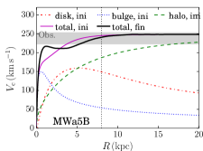
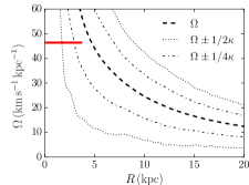
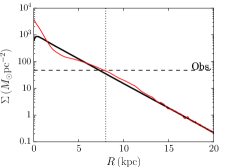
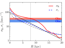
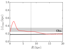
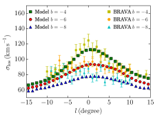
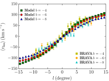
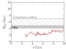
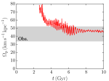
Figure 1: Results of Model a5B. (a) Initial and final rotation curves. (b) Angular frequencies of the disc (black curves) and bar (red line) at 10 Gyr. The length of the red line indicate the length of the bar. (c) Surface densities, and (d) radial and vertical velocity dispersion of the disc. (e) Total (disc, bulge, and dark-matter) density within $|z|<1.1$ kpc ($K_{z}$) at 10 Gyr. Symbols with error bars indicate observations (Bovy & Rix, 2013). (f) Scale height of the disc. Black and color curves in panels (c), (d), and (f) indicate the initial and final (10 Gyr) distribution, respectively. (g) Line-of-sight velocity dispersion and (h) mean velocity of the bulge region ($R<3$ kpc) at 10 Gyr. Symbols with error bars are BRAVA data. (i) Bar length and (j) pattern speed of the bar as a function of time. Vertical dotted lines in panels (a) and (c)–(f) indicate 8 kpc from the galactic center.

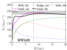
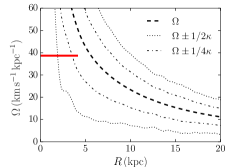
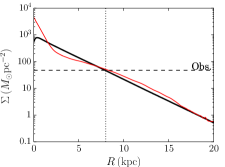
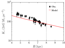
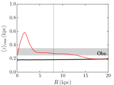
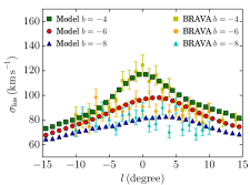
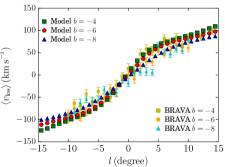
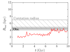
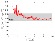
Figure 2: Same as Fig.1, but for model MWb6B.

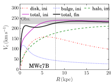
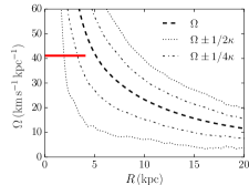
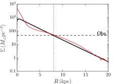
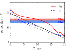
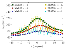
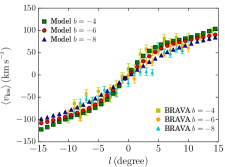
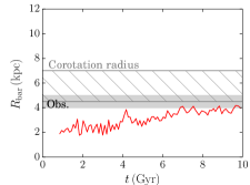
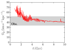
Figure 3: Same as Fig.1, but for model MWc7B.

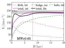
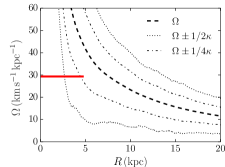
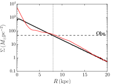
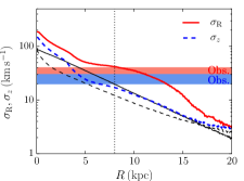
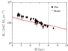
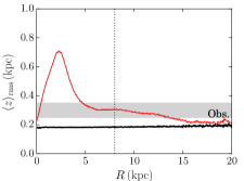
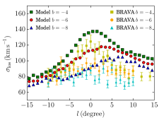
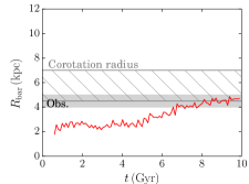
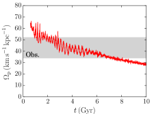
Figure 4: Same as Fig.1, but for model MWc0.65.

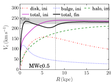
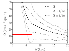
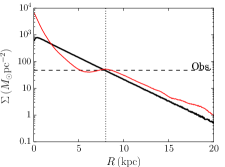
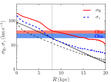
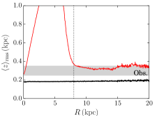
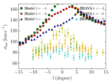
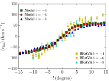
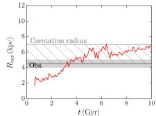
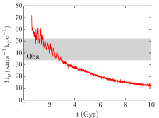
Figure 5: Same as Fig.1, but for model MWc0.5.

3 Results

Each model is simulated for 10 Gyr after which we compare the resulting disc and bulge structure with observations. The results of our simulations are shown in Figs. 1–5. The panels in the figures present, from the top-left to bottom-right,

1. the initial and final rotation curves,

2. angular frequency of the bar and disc at $t=10$ Gyr,

3. surface density profile,

4. disc radial and vertical velocity dispersion,

5. disc and dark-matter density within $|z|<1.1$ kpc ($K_{\rm z}/2\pi G$) (Kuijken & Gilmore, 1991),

6. disc scale height,

7. line-of-sight velocity dispersion of the bulge region ($R<3$ kpc),

8. mean line-of-sight velocity of the bulge region,

9. the time evolution of the bar length,

10. the time evolution of the bar’s pattern speed,

We also present the face- and edge-on views of models MWa5B, MWb6B, and MWc7B in Figure 6. Here, we assume that the bar angle with respect to the Sun-Galactic Center line ($\phi_{\rm bar}$) is $25^{\circ}$. In the edge-on view, we see a weak x-shaped bulge. The movies of the face-on view for these models are available as online materials.

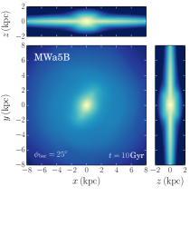
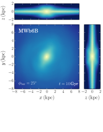
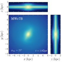
Figure 6: Face- and edge-on view at $t=10$ Gyr for models MWa5B, MWb6B, and MWc7B (from left to right). The Sun is located on the $y$-axis and the bar angle with respect to the Sun-Galactic Center line $\phi_{\rm bar}=25^{\circ}$.

3.1 Rotation curves

In panel (a) of Figs. 1–5, we present the circular velocity ($V_{\rm c}$) of the disc at $t=0$ (magenta) and at $t=10$ Gyr (black). The contributions of the individual components, at $t=0$, are shown in red (disc), blue (bulge), and green (halo). The grey shaded region indicates the observed circular rotation velocity at the Sun’s location, $238\pm 15$ km s^-1 (Bland-Hawthorn & Gerhard, 2016). The vertical dotted line marks the distance of 8 kpc from the centre. We measure $V_{\rm c}$ at $t=10$ Gyr using the centrifugal force calculated in the simulation. For the initial conditions, $V_{\rm c}$ is calculated using the assumed potential.

Compared with the initial conditions, the circular velocity at 8 kpc drops at the end of the simulation ($t=10$ Gyr) for nearly all the models shown here. The size and depth of the dip in the rotation curve correspond to the strength of the bar (see models MWc7B, MWc0.65, and MWc0.5). As the simulation progresses the shape of the rotation curve in the inner region changes, and the final curve has a peak at a few kpc from the Galactic centre. Compared to the rotation curve observed in the inner region such as in Sofue (2012), our peak is less high. The higher peak in the observations is, however, obtained by measurements of the H1 gas velocity. The clumps of gas in the inner region of the Galactic disc could have a higher line-of-sight velocity due to their motion along the bar, and the actual circular velocity might be lower than that obtained from the gas velocity (Baba et al., 2010). We, therefore, discuss the circular velocity at 8 kpc, but not the shape of the curve in the inner region. The measurements of the circular velocity at 8 kpc ($V_{\rm c,8kpc}$) for $t=10$ Gyr are summarized in Tables 3 and 7.

3.2 Halo spin

We find that halo spin is one of the most crucial parameters in order to reproduce the MW Galaxy. The halo spin parameter strongly affects the bar evolution. In general, bars grow longer by transferring their angular momentum to the halo, and the pattern speed slows down (Athanassoula, 2002). If the halo initially has a spin then the pattern speed of the bar increases and the bar length becomes shorter as the halo spin increases (Long et al., 2014; Fujii et al., 2018). For model MWc, we adopt a range of different halo spin parameters where we keep the other parameters fixed. As is shown in Figs. 3–5, the bars in the lesser ($\alpha_{\rm h}=0.65$) and no spin ($\alpha_{\rm h}=0.5$) cases evolve much stronger compared to the case with $\alpha_{\rm h}=0.8$. In Fig. 7, we present the surface density of these models at $t=10$ Gyr. Without halo spin, we see an x-shaped bulge that is much stronger than observed in the MW (Wegg & Gerhard, 2013). The effect of the halo spin can also be seen in the bulge kinematics, where the line-of-sight velocity dispersion of the bulge region becomes much higher than in the models without halo spin.

Our results indicate that an initial spin parameter of $\alpha_{\rm h}\sim 0.8$, which corresponds to $\lambda\sim 0.06$, matches the observations best. This value is consistent with the value observationally estimated for disc galaxies with a short bar (smaller than a quarter of the disc outer radius) (Cervantes-Sodi et al., 2013). We further investigated a model with a larger halo spin, but the result was not significantly different from those of a model with $\alpha_{\rm h}\sim 0.8$ (see Appendix C). From this result, we expect that a fixed potential case would be similar to the maximum halo spin cases because in both cases net angular momentum transfer from disk to halo is forbidden. We therefore adopt $\alpha_{\rm h}\sim 0.8$ for most of our models without explicitly indicating it in their name.

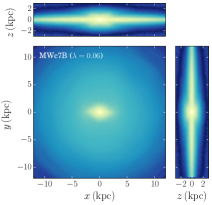
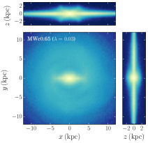
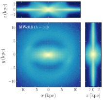
Figure 7: Surface density maps at $t=10$ Gyr for models MWc7B, MWc0.65 and MWc0.5 (left to right).

3.3 Comparison with disc observations

In order to evaluate the differences between models and observations, we use the stellar surface density of the disc ($\Sigma_{\rm 8kpc}$), radial velocity dispersion ($\sigma_{R,{\rm 8kpc}}$), and disc and dark-matter density within $|z|<1.1$ kpc ($K_{z,{\rm 8kpc}}$) at 8 kpc from the Galactic center. Hereafter, we assume that the Sun is located at 8 kpc from the Galactic centre.

In panel (c) we present the disc surface density profile at the start of the simulation (black curve) and at the end of the simulation ($t=10$ Gyr, red curve). The vertical dotted line indicates the location of the Sun, and the horizontal dashed line the surface density of the Galactic disc observed in the solar neighbourhood; $47.1\pm 3.4M_{\odot}$ pc^-2 (McKee et al., 2015; Bland-Hawthorn & Gerhard, 2016). Compared to the initial density profile, the central density increases and the surface density around the bar end drops slightly at $t=10$ Gyr. The density increases again in the region outside the bar length. Since we configured our models to form a bar with a length of $\lesssim 5$ kpc, the surface density at 8 kpc at $t=10$ Gyr is always larger than the initial value.

The initial surface density at 8 kpc depends on both the disc mass ($M_{\rm d}$) and the disc scale length ($R_{\rm d}$). The scale length is, however, limited by observations to $R_{\rm d}\sim 2.6$ kpc (Bland-Hawthorn & Gerhard, 2016). We tested the correlation between the disc mass ($M_{\rm d}$) and the surface density at 8 kpc at $t=10$ Gyr ($\Sigma_{\rm 8kpc}$). The results are shown in Fig. 8. The correlation coefficient between $M_{\rm d}$ and $\Sigma_{\rm 8kpc}$ is 0.82. Based on this result we set the disc mass of our models to $\sim 3.7\times 10^{10}M_{\odot}$.

We further find a weak correlation between the initial bulge scale length ($r_{\rm b}$) and $\Sigma_{\rm 8kpc}$ (with a coefficient of $-0.63$) and between the initial bulge characteristic velocity ($\sigma_{\rm b}$) and $\Sigma_{\rm 8kpc}$ (with a coefficient of 0.60), see Figs. 9 and  10. If we focus on models with $M_{\rm d}\sim 3.7M_{\odot}\times 10^{10}$ (black circles in the figures), we find that $r_{\rm b}\sim 1$ kpc and $\sigma_{\rm b}\sim 300$ km s^-1 gives a stellar surface density of the disc (at 8 kpc) which is similar to the observations.

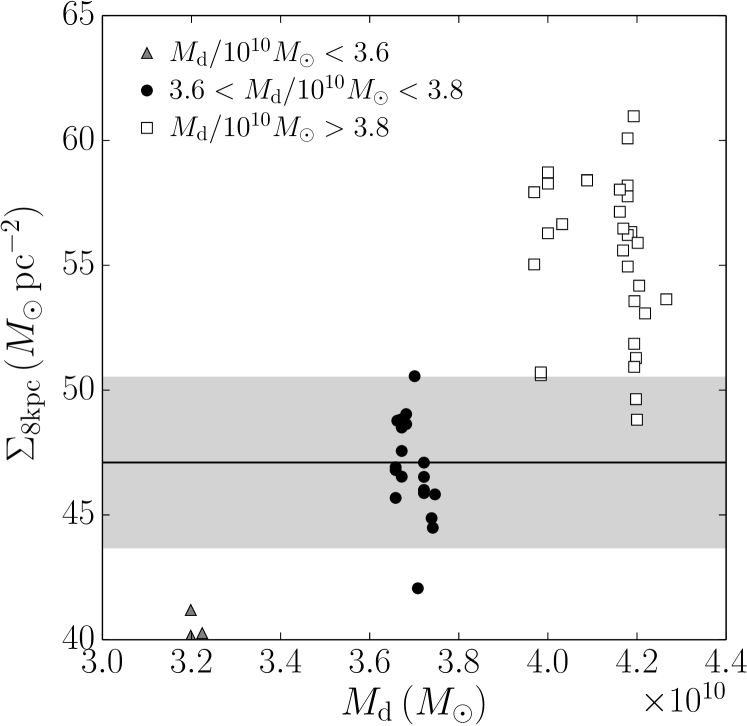
Figure 8: Relation between the disc mass and the disc surface density at 8 kpc at $t=10$ Gyr. Each symbol indicates one model. The black line and grey shaded region mark the observed value; $47.1\pm 3.4M_{\odot}$ pc^-2 .

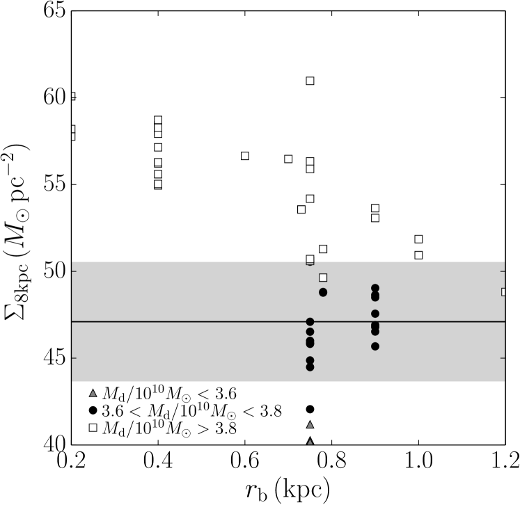
Figure 9: Relation between the bulge scale length and the disc surface density at 8 kpc at $t=10$ Gyr. The black line and grey shaded region mark the observed value; $47.1\pm 3.4M_{\odot}$ pc^-2 .

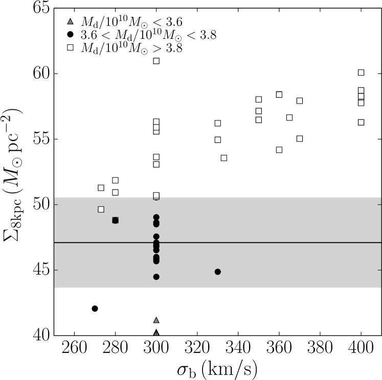
Figure 10: Relation between the bulge characteristic velocity and the disc surface density at 8 kpc at $t=10$ Gyr. The black line and grey shaded region mark the observed value; $47.1\pm 3.4M_{\odot}$ pc^-2 .

Now we investigate the relation between the initial parameters and the final velocity dispersion of the disc. The radial (red solid line) and vertical (blue dashed line) velocity dispersion of the disc at $t=10$ Gyr are presented in panel (d). In the same panel, we present the observed radial (red shaded) and vertical (blue shaded) velocity dispersion of the MW disc in the solar neighbourhood, $35\pm 5$ and $25\pm 5$ km s^-1, respectively (Bland-Hawthorn & Gerhard, 2016). Black curves in the same panel indicate the initial distributions. Both the radial ($\sigma_{R}$) and vertical ($\sigma_{z}$) velocity dispersion increase after the bar formation. When we look at our simulations we see that the ratio between the radial and vertical velocity dispersion is always larger than the observed ratio. This might be due to the lack of gas in our simulation. The vertical velocity dispersion can be increased by massive objects in the disc such as giant molecular clouds rather than spiral arms (Carlberg, 1987; Jenkins & Binney, 1990; Binney & Tremaine, 2008). We, therefore, ignore the vertical velocity dispersion when we tune our models to match with observations.

We find a correlation between $\sigma_{R}$ at 8 kpc ($\sigma_{R,{\rm 8kpc}}$) and the disc mass fraction ($f_{\rm d}$) with a correlation coefficient of 0.85 for models with $3.6\times 10^{10}M_{\odot}<M_{\rm d}<3.8\times 10^{10}M_{\odot}$ and 0.80 for all other models. This correlation is presented in Fig. 11. A larger $f_{\rm d}$ results in earlier bar formation (Fujii et al., 2018), which causes the velocity dispersion to increase as $f_{\rm d}$ increases. The results of Fig. 11 indicate that $0.4\lesssim f_{\rm d}\lesssim 0.45$ should be chosen to best agree with observations.

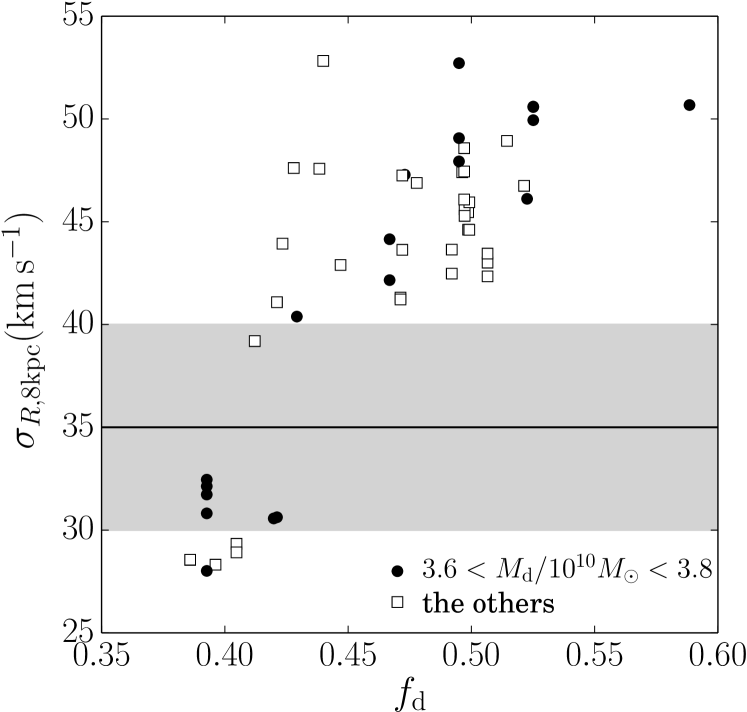
Figure 11: Relation between the disc mass fraction at $2.2R_{\rm d}$ ($f_{\rm d}$) and $\sigma_{R}$ at 8 kpc. Black line and grey shaded region indicate the observed value; $35\pm 5$ km s^-1.

We also find an anti-correlation between $K_{z}$ and $f_{\rm d}$. In panel (e) we plot $K_{\rm z}$ (Kuijken & Gilmore, 1991) at the end of the simulation ($t=10$ Gyr, red line). The black circles, with error bars are observed values taken from (Bovy & Rix, 2013). The vertical dotted line marks the location of the Sun at 8 kpc from the Galactic centre. We take $K_{\rm z}/2\pi G=70\pm 5$ ($M_{\odot}\,{\rm pc}^{-2}$) at 8 kpc as the observed value (Bland-Hawthorn & Gerhard, 2016).

The value of $K_{Z}$ should depend on both the disc and halo structure. We evaluated the correlation between $K_{z}$ and all initial parameters in Fig. 12. When we look at the models with similar disc mass ($3.6\times 10^{10}M_{\odot}<M_{\rm d}<3.8\times 10^{10}M_{\odot}$) we find an anti-correlation of -0.86 between $K_{z}$ and the disc mass fraction ($f_{\rm d}$). This plot suggests that $0.40<f_{\rm d}<0.55$ results in a good fit to the observations. Thus, both $\sigma_{R}$ and $K_{z}$ at 8 kpc suggest $f_{\rm d}\sim 0.4$–0.45.

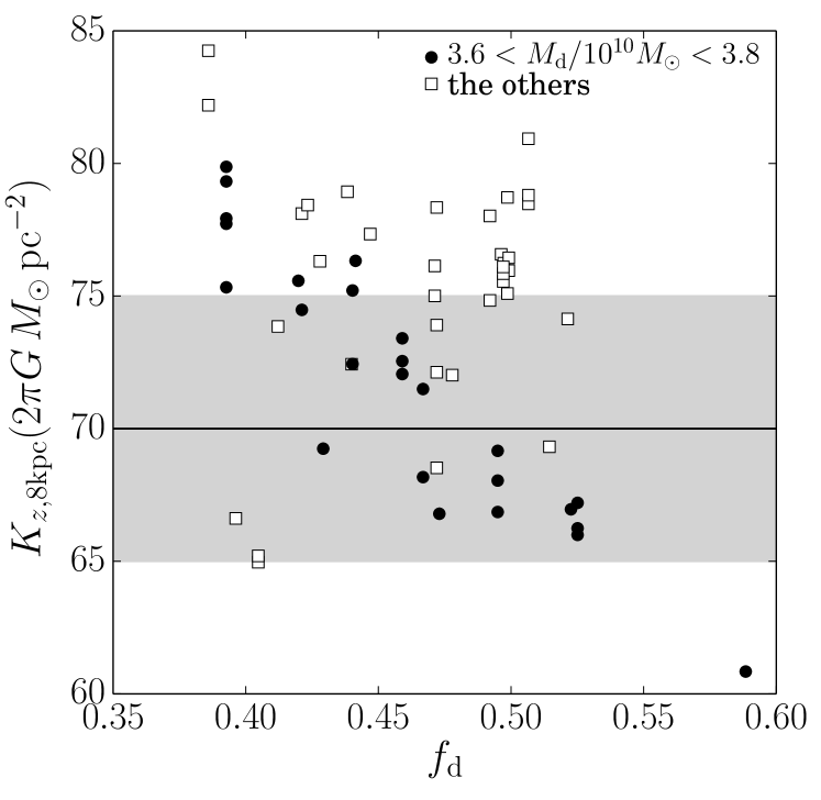
Figure 12: Relation between the disc mass fraction at $2.2R_{\rm d}$ ($f_{\rm d}$) and $K_{z}$ at 8 kpc. Black line and grey shaded region indicate the observed value; $K_{\rm z}/2\pi G=70\pm 5$ (km s^-1).

We measure the disc scale height by taking the root mean square of the disc particles $z$ coordinate. The results are presented in panel (f) for $t=0$ (black line) and $t=10$ Gyr (red line). The scale height of the MW disc is measured to be $0.30\pm 0.05$ kpc (Bland-Hawthorn & Gerhard, 2016) and indicated by the grey shaded area. Galactic discs thicken due to the heating induced by the bar and spiral arms and in the inner regions where the bar develops the scale height is significantly larger. We find that if the initial scale height is set to 0.2–0.3 kpc, the final disc scale height, for models with a halo spin, fall within the observed range at $\sim 8$ kpc. For the models without halo spin, the bar’s strong dynamical heating causes the scale height to become too high, even in the bar’s outer region. For the same reason as for the vertical velocity dispersion of the disc, we do not consider matching the disc scale height with the observations when we tune our models.

Considering the above results, we conclude that $M_{\rm d}\sim 3.7\times 10^{10}M_{\odot}$, $r_{\rm b}\sim 0.7$–1.0 kpc, $\sigma_{b}\sim 300$ km s^-1, and $f_{\rm d}\sim 0.45$ are necessary for the MW model. The values of $\Sigma_{\rm 8kpc}$, $\sigma_{R,{\rm 8kpc}}$, $\sigma_{z,{\rm 8kpc}}$, $K_{z}$, and $V_{\rm c,8kpc}$ are summarized in Tables 3 and 7.

3.4 Comparison with bulge kinematics observations

The kinematics of the bulge region is another data point that can be compared with available observational data. We, therefore, compare our simulations with the bulge kinematics obtained from the BRAVA observations (Kunder et al., 2012). This gives the line-of-sight velocity and the velocity dispersion at the Galactic center for $b=-4^{\circ}$, $-6^{\circ}$, and $-8^{\circ}$ as a function of $l$. We “observe” our simulated galaxies at $t=10$ Gyr. To perform these observations we set the observation angle with respect to the bar to $\phi_{\rm b}=25^{\circ}$. In panels (g) and (h), we present the line-of-sight velocity and its dispersion as a function of $l$ for both the simulations and observations. The BRAVA data is represented by the yellow squares, orange circles, and cyan triangles. The simulation data is presented by the green squares, red circles and blue triangles. The observation angle to the bar ($\phi_{\rm b}=25^{\circ}$) is motivated by observations that put it at $\sim 20^{\circ}$–$40^{\circ}$ (López-Corredoira et al., 2005; Cao et al., 2013; Wegg & Gerhard, 2013; Bland-Hawthorn & Gerhard, 2016). However, recent analysis suggests an angle closer to $40^{\circ}$ (Ciambur et al., 2017). We, therefore, performed additional analysis where we used $30^{\circ}$ and $40^{\circ}$ angles, but the differences were minor and consistent with those of Shen et al. (2010).

In order to evaluate the match between observations and simulations, we adopt the method used in Abbott et al. (2017) and Gardner et al. (2014), in which the $N$-body simulations are compared with the BRAVA observations. We measure $\chi^{2}$ for $v_{\rm los}$ and $\sigma_{los}$ for $b=-4^{\circ}$, $-6^{\circ}$, and $-8^{\circ}$, respectively. Here we calculate

$$\chi^{2}_{a}=\sum^{N_{\rm data}}_{i}\left(\frac{a_{{\rm sim},i}-a_{{\rm obs},i}}{\sigma_{{\rm obs},i}}\right)^{2},$$ (7)

where $a_{\rm sim}$ and $a_{\rm obs}$ are data points obtained from simulations and observations, and $\sigma_{\rm obs}$ is the observational error for $a_{\rm obs}$. The $\chi^{2}$ values for $v_{\rm los}$ and $\sigma_{\rm los}$ are shown in Fig. 15, where the value is normalized by the number of the data points.

We did not find any strong correlations with the initial condition parameters, but we found that a large disc mass fraction fits better with the observation of $\sigma_{\rm los}$. In Fig. 13 we present $\chi^{2}$ for $\sigma_{\rm los}$ (sum of $\chi^{2}$ for $b=-4^{\circ}$, $-6^{\circ}$, and $-8^{\circ}$ between $l=-20^{\circ}$ to $l=20^{\circ}$ normalized by the number of the data points, $N_{\rm data}=63$) as a function of $f_{\rm d}$. This figure suggests that $f_{\rm d}\gtrsim 0.4$. This is simply because a stronger bar with a smaller $f_{\rm d}$ heats the bulge as well as the disc. Bulge line-of-sight velocity, on the other hand, shows the rotation speed, which is barely affected by the heating induced by the bar.

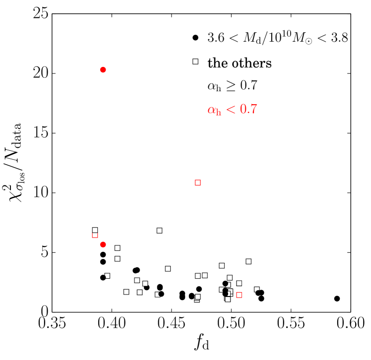
Figure 13: $\chi^{2}$ for $\sigma_{\rm los}$ as a function of $f_{\rm d}$. The value of $\chi^{2}_{\sigma_{\rm los}}$ for model MWc0.5 is 91.4, and therefore not shown in this panel.

3.5 Bar length and pattern speed

The bar’s length and pattern speed are also important values to characterize the structure of a galactic disc. We use the same method as Fujii et al. (2018) to measure the length of the bar (see also Okamoto et al., 2015). We first perform a Fourier decomposition of the disc’s surface density:

$$\frac{\Sigma(R,\phi)}{\Sigma_{0}(R)}=\sum_{m=0}^{\infty}A_{m}(R){\rm e}^{{\rm i}m[\phi-\phi_{m}(R)]}$$ (8)

where $A_{m}(R)$ is the Fourier amplitude and $\phi_{m}(R)$ is the phase angle for the $m$-th mode. Using the $m=2$ component and $\Delta R=1$ kpc radial bins we compute the phase angle ($\phi_{2}$) and amplitude ($A_{2}$) of the bar for each radius up to 20 kpc. The radius with the highest amplitude value ($A_{\rm 2,max}$) is defined as the bar’s phase angle ($\phi_{\rm 2,max}$). Then, starting at the radius for which we obtained $A_{\rm 2,max}$, we measure the phase angle to each outer radial bin. The bin for which the difference with $\phi_{\rm 2,max}$ is $\Delta\phi>0.05{\rm\pi}$ defines the bar length ($R_{\rm b}$). The result is shown using the red line in panel (i) of Figs. 1–5. In this panel, the grey shaded region indicates the co-rotation radius (4.5–7.0 kpc) as suggested by observations (Bland-Hawthorn & Gerhard, 2016). Because a bar cannot be longer than the co-rotation radius (Contopoulos, 1980; Athanassoula, 1992), it must be shorter than the grey shaded region.

As is suggested by previous simulations (Long et al., 2014), the halo spin parameter influences the bar length and the pattern speed the most. For the models with the strongest halo spin ($\alpha_{\rm h}=0.8$), the final bar length ($\sim 4$ kpc) is slightly shorter than the co-rotation radius. For the models with a weak halo spin ($\alpha_{\rm h}=0.65$) the final bar length is slightly longer and reaches the lower limit of the co-rotation radius ($4.5$ kpc). In the models without halo spin, the bar continues to develop and the final length exceeds 6 kpc. This is much longer than what observations suggest. Estimates for the MW bar length, obtained from a model fit to near-IR star count, are $5.0\pm 0.2$ kpc (Wegg et al., 2015; Bland-Hawthorn & Gerhard, 2016) and $\sim 4$ kpc (Ciambur et al., 2017). Our measured bar length ($\sim 4$ kpc) is consistent with these observations. We note that the used measurement method affect the resulting bar lengths. In a method that uses the $m=2$ mode, the obtained bar length tends to be shorter compared to other radial profile methods (Wegg et al., 2015).

The bar’s pattern speed is presented in panel (j) of Figs. 1–5. This is obtained by computing the phase of the bar ($\phi_{\rm 2,max}$), for each snapshot, using the Fourier decomposition (Eq. 8). The angular speed is then determined by computing the difference between the snapshots and presented using the red curve. In this panel, the grey shaded region marks the observed pattern speed of the Galactic bar, $\Omega_{\rm p}=43\pm 9$km s^-1 (Bland-Hawthorn & Gerhard, 2016), although the pattern speed is still under debate (Monari et al., 2017; Pérez-Villegas et al., 2017; Hattori et al., 2018). For models with $\alpha_{\rm h}=0.8$, the final pattern speed stabilizes within the grey area, but for models with $\alpha_{\rm h}=0.65$ (moderate spin) and 0.5 (no spin), the pattern speed drops below the observational constraints. In Appendix C, we show more extreme cases (negative and maximum spins). With a negative spin the final pattern speed is even slower than the case without spin. With the maximum spin, the pattern speed was comparable to the case with $\alpha_{\rm h}=0.8$ or even larger. Thus, the pattern speed also indicates that $\alpha_{\rm h}\sim 0.8$. For our models in which the bulge kinematics fit the observations, the final speed of the bar was 40–50 km s^-1. As far as we tested, no model has a pattern speed faster than $\sim$50 km s^-1.

We define the final pattern speed as the averaged pattern speed over the last 10–20 snapshots. The results are 45, 38, and 40 km s^-1 for models MWa5B, b6B, and c7B, respectively. The time-scale for the 10–20 snapshots covers the oscillation period of the bar’s pattern speed. The measured pattern speeds are summarized in Tables 3 and 7. We discuss the oscillation of the bar’s pattern speed further in Sect. 4.

When we compare the final pattern speed of the bar for models with a different number of particles ($N$) we see that it is not exactly the same (Table 3). This could be caused by resolution differences or run-to-run variations (Sellwood & Debattista, 2009). In order to determine if the difference is caused by $N$ or by run-to-run variations, we perform four runs for the same initial parameters. The runs differ in $N$ and in the random seed used to generate the initial particle positions and velocities. The results are summarized in Appendix B. For our tests the bar’s pattern speed varied by a few km s^-1 for the models with $N\sim$100M. For the $N\sim$1B models the run-to-run variation is smaller, $\sim$1 km s^-1.

Except for the halo spin, it is unclear which parameter directly influences the pattern speed of the bar. In Fig. 14, we observe a weak dependence on the disc-mass to total-mass fraction, $f_{\rm d}$. We find that the bar speed drops slightly when $f_{\rm d}$ increases. For $f_{\rm d}\sim 0.45$, the expected pattern speed is 40–50 km s^-1. In addition, we did not see any model with a bar pattern speed faster than $\sim 50$ km s^-1 in our simulations.

We further measure the co-rotation radius ($R_{\rm CR}$), and the inner ($R_{\rm ILR}$) and outer ($R_{\rm OLR}$) Lindblad resonance radii. These values are presented in columns 8, 9 and 10 of Tables 3 and 7. Models MWa and a5B have a relatively fast rotating bar, and therefore the $R_{\rm OLR}$ is $\sim 9$ kpc, but for models MWb, b6B, c0.8, and c7B we find $R_{\rm OLR}\sim 10$ kpc. For both models, the location of the outer Lindblad resonances was further out than the Galactic radius of the Sun.

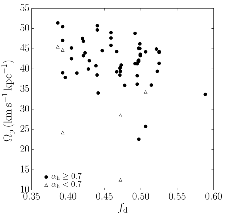
Figure 14: Relation between the initial disc mass fraction and the bar’s pattern speed at $t=10$ Gyr.

3.6 Best-fitting models

In order to evaluate the comparison between models and observations, we also calculate $\chi^{2}$ (see Eq. 7) for $\Sigma$, $\sigma_{R}$, $K_{z}$ at 8 kpc, which are $\chi_{\Sigma}^{2}$, $\chi_{\Sigma_{R}}^{2}$, and $\chi_{K_{z}}^{2}$. The results for the best fitting models are summarized in Table 4 and Fig. 15. The results for all models are presented in Table 8. Models MWa, b, and c0.8 are models for which the sum of all $\chi^{2}$ is relatively small, where MWa/a5B have the smallest $\chi^{2}$ value. The total $\chi^{2}$ of model MWb/b6B is not the smallest, but the $\chi^{2}$ for $\sigma_{\rm los}$ is the smallest. For model MWc0.8/MWc7B, the sum of $\chi_{\Sigma}^{2}$, $\chi_{\Sigma_{R}}^{2}$, and $\chi_{K_{z}}^{2}$ is $\sim 5.5$, but the sum of $\chi^{2}_{v_{\rm los}}$ and $\chi^{2}_{\sigma_{\rm los}}$ is the smallest. Without halo spin, the $\chi^{2}$ values are very large (see model MWc0.5). This is the reason we showed these models in detail in Figs. 1–3. In the discussion section, we describe these models in more detail.

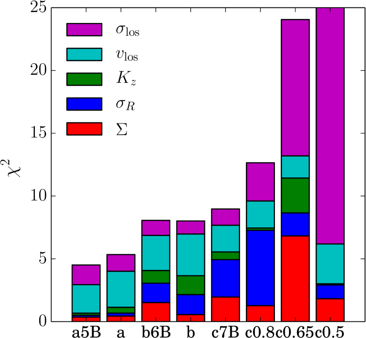
Figure 15: $\chi^{2}$ for all models listed in Table 1. The total $\chi^{2}$ value for model MWc0.5 is 97.6. .

Summarizing the results of the previous sections we conclude that the following parameters for the initial conditions lead to the best-fitting models. For the disc mass, the best fit value is $M_{\rm d}\sim 3.70\times 10^{10}M_{\odot}$. With an initial $Q$ at $2.5R_{\rm d}$ of 1.2, this leads to a central velocity dispersion for the disc of $\sigma_{R0}\sim 90$ km s^-1. Compared to the disc the parameters for the bulge are less clear. We find that $r_{\rm b}\sim 0.7$–1.0 kpc and $\sigma_{b}\sim 300$ km s^-1 fit the observations and result in $M_{\rm b}=3$–$5\times 10^{9}M_{\odot}$, assuming a Hernquist model. If we calculate the bulge-to-disc mass ratio, it is $\sim 0.07$–0.15. In contrast to the result of Shen et al. (2010), we find that it is not necessary to have a bulge-to-disc mass ratio that is smaller than 0.08.

The halo spin is a very important parameter. For the best-fitting models, the halo spin parameter was $\alpha_{\rm h}=0.8$, which corresponds to $\lambda\sim 0.06$. This is larger than the median value obtained from cosmological $N$-body simulations, $\lambda=0.03$–0.04 (Bett et al., 2007). However, the spin parameters obtained from cosmological simulations have a significant amount of dispersion. The found $\lambda\sim 0.06$ is, therefore, not an extremely large value. All models with a smaller or even no preferential spin give a bar pattern speed that is too slow (at 10 Gyr). This result suggests that the MW halo initially had a significant amount of rotation. The final value of the spin parameter was $\sim 0.07$ for models MWa5B, MWb6B, and MWc7B. This value is slightly higher than the observationally suggested spin parameter for short barred galaxies ($\lambda=0.061$), but still comparable (Cervantes-Sodi et al., 2013). In Appendix C, we summarized the final spin parameters for the other models.

We further find that disc-to-total mass fraction ($f_{\rm d}$) is an important parameter. This parameter controls the bar formation epoch, which corresponds to the opposition against bar instability (Fujii et al., 2018). If $f_{\rm d}$ is larger, the bar forms earlier and grows stronger. Since $\sigma_{R,{\rm 8kpc}}$ and $K_{z,{\rm 8kpc}}$ correlate and anti-correlate with $f_{\rm d}$, the preferable value of $f_{\rm d}$ is $\sim 0.45$. The line-of-sight velocity dispersion in the bulge region also indicates $\sim 0.45$ as preferable value.

Table 3: Disc properties for the simulated galaxies at 10 Gyr

Model	$\Sigma_{\rm 8kpc}$	$\sigma_{R,{\rm 8kpc}}$	$\sigma_{z,{\rm 8kpc}}$	$K_{z,{\rm 8kpc}}$	$V_{\rm c,8kpc}$	$\Omega_{\rm b}$	$R_{\rm CR}$	$R_{\rm OLR}$	$R_{\rm ILR}$
	($M_{\odot}\,{\rm kpc}^{-2}$)	(km s-1)	(km s-1)	($2\pi G\,M_{\odot}\,{\rm kpc}^{-2}$)	(km s-1)	(km s-1 kpc-1)	(kpc)	(kpc)	(kpc)
MWa5B	45.1	36.9	14.6	72.1	241	46	4.7	9.1	1.7
MWa	44.8	37.4	14.9	73.4	241	48	4.4	8.5	1.6
MWb6B	51.3	41.2	15.8	75.0	230	38	5.6	10.1	1.9
MWb	49.6	41.3	15.9	76.1	230	40	5.4	9.8	1.8
MWc7B	51.9	43.6	16.3	73.9	228	40	5.2	9.8	1.9
MWc	50.9	47.3	17.2	72.1	226	39	5.3	10.1	2.0
MWc0.65	56.0	41.8	17.2	78.3	226	28	7.9	15.7	2.7
MWc0.5	51.7	40.2	18.8	68.5	214	12	18.6	30.0	5.5

The first column indicates the name of the model. Columns 2–6 give the surface density, radial and vertical velocity dispersion, vertical force at $z=1.1$ kpc, and circular velocity at $R=8$ kpc. The seventh column gives the pattern speed of the bar. Column 8–10 show the corotation, outer and inner Lindblad resonance radii.

Table 4: $\chi^{2}$ for $\Sigma_{\rm 8kpc}$, $\sigma_{R,{\rm 8kpc}}$, $K_{z,{\rm 8kpc}}$, $v_{\rm los}$, and $\sigma_{\rm los}$ at 10 Gyr

Model	${\Sigma_{\rm 8kpc}}$	$\sigma_{R,{\rm 8kpc}}$	$K_{z,{\rm 8kpc}}$	$v_{\rm los}$	$\sigma_{\rm los}$	total
MWa5B	0.4	0.1	0.2	2.3	1.6	4.5
MWa	0.4	0.2	0.5	2.9	1.3	5.3
MWb6B	1.5	1.5	1.0	2.8	1.2	8.1
MWb	0.6	1.6	1.5	3.3	1.0	8.0
MWc7B	2.0	3.0	0.6	2.1	1.3	9.0
MWc0.8	1.3	6.0	0.2	2.2	3.0	12.6
MWc0.65	6.8	1.8	2.8	1.8	10.9	24.1
MWc0.5	1.8	1.1	0.1	3.2	91.4	97.6

4 Discussion

Here we “observe” our best-fitting models, and discuss the origin of structures observed in the MW galaxy.

4.1 Inner bar structure

Using the ESO Vista Variables from the Via Lactea survey (VVV), Gonzalez et al. (2011) traced the bar structure of the Galactic centre. They counted the number of clumps with red stars for each galactic longitude bin ($|l|<\pm 10^{\circ}$) for $b=\pm 1^{\circ}$ as a function of the $K$ magnitude. They converted the magnitude into the distance from the Sun and used this to measure the distance to the peak of the distribution of red clumps, and assumed that the peaks trace the Galactic bar. In order to reproduce this measurement, we use disc and bulge particles instead of red clumps. In each ($l$, $b$) bin, we count the number of stars as a function of the distance from the Sun ($d$) and measure the peak distance. In Fig. 16 we present the results for the $\phi_{\rm bar}=25^{\circ}$ and $40^{\circ}$ view angles. Similar to the results of Gonzalez et al. (2011) and also Zoccali & Valenti (2016), we “observe” bars much more inclined than the assumed bar angle and the bar angle changes between $|l|=$5–10^∘. This is due to the projection effect and the existence of the bulge which was nicely shown, using $N$-body simulations, by Gerhard & Martinez-Valpuesta (2012). The points in which the bar breaks (i.e., the outer edge of the “inner bar”) only barely depends on the bar’s viewing angle ($\phi_{\rm bar}$).

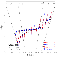
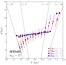
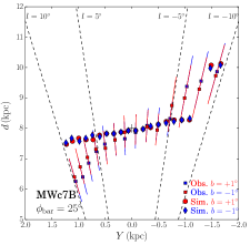
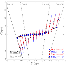
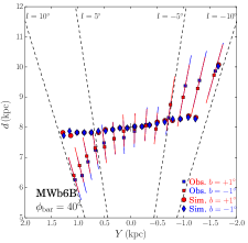
Figure 16: Position of the Galactic bar with respect to the Sun, traced via the density peaks (similar to Fig. 3 of Gonzalez et al., 2011; Zoccali & Valenti, 2016) for models MWa5B (left), MWb6B (middle), and MWc7B (right). The bar angle is set to be $\phi_{\rm bar}=25^{\circ}$ (top) and $40^{\circ}$ (bottom). The Sun is located on the $y$-axis.

4.2 Hercules stream in simulated galaxies

There are some known structures in the velocity space distribution of solar neighbourhood stars. One of the most significant structures is the Hercules stream (Dehnen, 1998, 2000): a co-moving group of stars with $30$–$50$ km s^-1 slower than the velocity of the local standard of rest ($V_{\rm LSR}$) and with $U<0$ km s^-1 (Dehnen, 2000; Quillen et al., 2018). In a stellar number distribution, as a function of $V$, the Hercules stream appears as a second peak at $-30$ to $-50$ km s^-1 from the main peak (Francis & Anderson, 2009; Monari et al., 2017).

The origin of the Hercules stream is not yet completely clear. Dehnen (2000) suggested that it is caused by the outer Lindblad resonance (OLR) (see also Antoja et al., 2014; Monari et al., 2017; Hunt et al., 2018b). For this model, a fast bar ($\gtrsim 50$ km s^-1 kpc^-1) is required to bring the OLR radius near the Sun. Pérez-Villegas et al. (2017), on the other hand, suggested that the Hercules stream is caused by resonant stars between the co-rotation and OLR radii. For this model a slower bar ($\sim 40$ km s^-1 kpc^-1) is suggested. In addition, Hattori et al. (2018) recently suggested a model in which a slow bar (36 km s^-1) combined with spiral arms can reproduce the Hercules stream. However, they also found that just a fast bar, or both a fast bar and spirals can reproduce the Hercules stream. Hunt & Bovy (2018) explained the Hercules stream using a 4:1 OLR of a slow bar. The above studies assume a fixed potential for the bar and spiral arms. Hunt et al. (2018a), on the other hand, showed that it can be reproduced by transient spirals only. Using ‘live’ $N$-body simulations, Quillen et al. (2011) studied the existence of the Hercules stream. They concluded that a Hercules-like stream appears outside of the OLR and with $\phi_{\rm b}=45^{\circ}$ when the spiral arm configuration is similar to the one observed. In this section we investigate Hercules-like streams in our $N$-body models.

Our MWa5B model has the fastest bar pattern speed (45 km s^-1 kpc^-1) and the resulting OLR radius is 9.1 kpc. For this model, we take the position of the Sun every 0.5 kpc between 7.5–11.5 kpc. The bar’s view angle is not fully determined from the observations, we, therefore, take angles between 20–40^∘ (Bland-Hawthorn & Gerhard, 2016). In Fig. 17 we present the surface densities in the $R$-$\phi$ plane for $t=9.82$–10.00 Gyr. In this figure, the surface density is normalized within each radial bin (i.e., the mean density at the radius is set to be 1). We also perform a Fourier decomposition (see equation 8) at each radius and include the $m=2$ and $m=4$ phases in the figure. These phases roughly trace the spiral arm positions. As is seen in the figure, the spiral structure changes significantly over time. The position of the Sun, $R\sim 8$ kpc and $\phi_{\rm b}\sim 20^{\circ}$–40^∘, falls mostly in the inter-arm regions.

In Fig. 18, we present the velocity distribution of stars that are within 0.5 kpc from the assumed position of the Sun. Here we take $R=7.5$ to $R=10$ kpc for every 0.5 kpc and from $\phi_{\rm bar}=20^{\circ}$ to $\phi_{\rm bar}=40^{\circ}$ for every $5^{\circ}$ as the position of the Sun. We show $t=9.99$ Gyr, in which the configuration of the spiral arms is similar to those observed in the MW disc. The Perseus arm at $\sim 10$ kpc and Scutum or Sagittarius arm at $\sim 6$ kpc from the Galactic centre (Reid et al., 2014; Vallée, 2017). In simulations $-v_{R}$, where $v_{R}$ is the radial velocity, is equivalent to $U$ in observations. For the tangential velocity ($v_{\phi}$), $v_{\phi}-V_{\rm LSR}$ is equivalent with $V$. We use the circular velocity at 8 kpc ($v_{\rm circ,8kpc}=241$ km s^-1 for this model) as $V_{\rm LSR}$. Hercules-like structures are unclear when only looking at the phase-space maps, and therefore we also present the number of stars for $v_{\rm R}>0$ as a function of $v_{\phi}-v_{\rm c,8kpc}$.

We detect the Hercules-like stream using a least-mean-square method. We fit the sum of two Gaussian functions to the distribution of stars with $v_{\rm R}>0$ using,

$$f(v_{R})=N_{1}\exp\left[-\frac{(v_{R}-v_{1})^{2}}{2\sigma_{1}^{2}}\right]+N_{2}\exp\left[-\frac{(v_{R}-v_{2})^{2}}{2\sigma_{2}^{2}}\right],$$ (9)

where $N_{1}$, $N_{2}$, $v_{1}$, $v_{2}$, $\sigma_{1}$, and $\sigma_{2}$ are fitting parameters, with $N_{1}>N_{2}$. We assume that a Hercules-like stream is detected when this function gives a better fit than a single Gaussian function and when the following conditions are satisfied:

1. $N_{2}>0.1N_{1}$

2. $-20<v_{1}<20$ km s^-1

3. $-60<v_{2}<-20$ km s^-1

4. $20<v_{1}-v_{2}<60$ km s^-1.

Using this function, we find two-peak structures when the Sun is located on the outer Lindblad resonance ($\sim 9$ kpc). We perform this fitting procedure for 40 different Sun locations ($7.0\leq R\leq 10.5$ kpc every 0.5 kpc and $20^{\circ}\leq\phi_{\rm bar}\leq 40^{\circ}$ every $5^{\circ}$). The locations in which a stream is found are indicated using the red and blue lines in Fig. 18.

These structures, however, are not always seen. In the top panels of Fig. 19 we present the velocity distribution of model MWa5B, assuming the position of the Sun is at $R=9.5$ kpc and $\phi_{\rm b}=20^{\circ}$ for $t=9.96$–10.00 Gyr. At this location we often detected the stream structure. Although Hercules-like structures are seen in $t=9.96$–9.98 Gyr, they are not seen at slightly different times such as $t=9.99$ and 10.00 Gyr, in which the location of the Sun is still between two major arms.

In order to quantify the frequency with which we “observe” the Hercules-like stream, we perform this fitting for the last 100 snapshots and present the frequency of the Hercules-like stream for models MWa5B and MWc7B in Figs. 20 and 21, respectively. We did not perform this analysis for model MWb6B because the OLR radius is very similar to that of model MWc7B. We find an enhancement of the streams frequency at a radius slightly further out than the OLR radius, namely at $R\sim 9$ and 10 kpc for models MWa5B and MWc7B, respectively. At this radius, we detect a Hercules-like stream in at most $\sim 50$ % of the snapshots. For model MWc7B, we further find a high stream frequency at $R=9$ kpc, which is between the co-rotation and OLR radius.

We further tested a situation where the Sun is located in an inter-arm region (Bland-Hawthorn & Gerhard, 2016), i.e., the local surface density is smaller than the mean density at the Galactocentric distance ($R$). The fraction of the inter-arm regions among the distributions in which a Hercules-like stream is detected is $\sim 60$ % and $\sim 70$ % for models MWa5B and MWc7B, respectively. Hercules-like streams, again, frequently appear at the OLR radii, and the maximum frequency is $\sim 50$ % among inter-arm regions for all the simulation times that we analyzed.

We also test the recent observation that finds the Hercules stream at the Galactic longitude of $l=270^{\circ}$ (Quillen et al., 2018). Fig. 19 therefore also shows the velocity distribution for model MWa5B at $R=9.5$ kpc where $l=0$, 90, 180, and $270\pm 45^{\circ}$ and $\phi_{\rm bar}=20^{\circ}$. These are the locations in which the Hercules-like streams most often appear (see Fig. 20). Indeed, the strength of the Hercules-like structure is different for each $l$, but there is no sign that a Hercules-like feature is seen more often for $l=270\pm 45^{\circ}$.

For the radii in which the stream frequency is high, we investigated the time dependence. In Fig.  22, we present the time at which we detected a Hercules-like stream for the last 100 snapshot ($\sim 1$ Gyr). The timing for which we “observe” Hercules-like streams is not periodically, but once they appear, they tend to continue for 20–30 Myr and sometimes even for $\sim 100$ Myr.

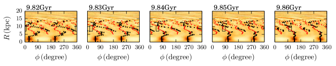
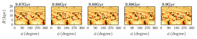
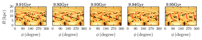
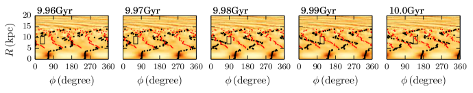
Figure 17: Surface density of model MWa5B at $t=9.82$–10.00 Gyr. The surface density is normalized by the average at each radius. The rectangle in each panel marks the region with $R=7$–10.5 kpc and $\phi_{\rm bar}=20$–40^∘. Black and red dots indicate the phase, determined using Fourier decomposition (Eq. 8), for $m=2$ and $m=4$, respectively.

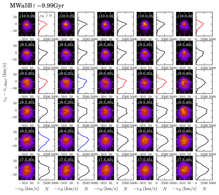
Figure 18: Velocity distribution of model MWa5B at $t=9.99$ Gyr. Hercules-like streams, detected using the least-mean-square fitting method, are marked by the red (in arm location i.e., higher surface density than the average at the radius) and blue lines (inter-arm i.e., lower surface density than the average), black lines indicate no detection.

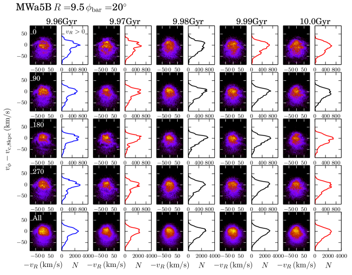
Figure 19: Time evolution of the velocity distribution for model MWa5B at $R=9.5$ kpc and $\phi_{\rm bar}=20^{\circ}$ for $t=9.96$–10.00 Gyr. From top to bottom, velocity distribution for $l=0$, 90, 180, $270\pm 45^{\circ}$, and all (total of the above). Red, blue and black lines are the same as those in Fig. 18

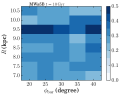
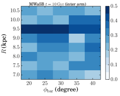
Figure 20: Stream frequency for the last 100 snapshots ($t=9.0$–$10.0$ Gyr) for model MWa5B. Left: irrespective of the position of spiral arms. Right: only for inter arm regions.

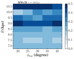
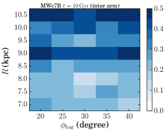
Figure 21: Same as Fig. 20, but for model MWc7B.

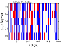
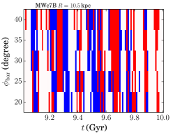
Figure 22: Stream appearances as a function of time for Models MWa5B $R=9.5$ kpc (left) and MWc7B $R=10.5$ kpc (right). The time interval of each snapshot is $\sim 10$ Myr. Red and blue indicate timings in which we detected a stream in the arm and inter-arm regions, respectively.

We repeat the above analysis for $t\sim 5$ Gyr, when the bar rotates faster than at $t=10$ Gyr and the pattern speed oscillates between 48–56 km s^-1. The corresponding OLR occurs at $R\sim 7.5$–9 kpc.

In Fig. 23 we present the surface density plots in the $R$-$\phi$ plane of model MWa5B for $t=5.00$–5.19 Gyr. In this figure, we see that the bar oscillates back and forth over a period of $\sim 200$ Myr. This oscillation corresponds to the oscillation in the pattern speed of the bar. The pattern speed of the bar reaches a minimum at $t=5$ Gyr. Then it gradually speeds up and reaches the local fastest velocity (56 km s^-1) at $t=5.08$ Gyr before it slows down again. At $t=5.16$ Gyr, the pattern speed again reaches the slowest phase (48 km s^-1). This oscillation seems to be due to the interaction with spiral arms as suggested by Sellwood & Sparke (1988) and also Baba (2015). Since the spiral arms outside the bar have a pattern speed slower than that of the bar, they repeatedly connect and disconnect. When the bar catches up with the outer spiral arms, the bar’s pattern speed is accelerated ($t=5.00$–5.08 Gyr) and reaches its maximum pattern speed at $t=5.08$ Gyr. Since the spiral arms move slower than the bar, the spirals start to get behind ($t=5.09$–5.15 Gyr) and detach from the bar at $t=5.16$ Gyr. During this process, the bar slows down and reaches the slowest pattern speed at $t=5.16$ Gyr. After that the bar connects to the spiral arms which are ahead of the bar ($t=5.17$–5.19 Gyr). This oscillation becomes weaker with time, but continues until the end of the simulation. We therefore also see this oscillation around 10 Gyr (see Fig. 17), although it is much weaker than at 5 Gyr.

In Fig. 24, we present the velocity distribution at $t=5.17$ Gyr for $R=7.5$–10 kpc and $\phi_{\rm bar}=20$–40^∘. At these times, the position of the Sun is between two major spiral arms. The figures contain more structures in the velocity distribution than those seen at $\sim 10$ Gyr. The difference appears to be caused by the existence of stronger spiral structures at $\sim 5$ Gyr. Quillen et al. (2011) showed that the velocity distribution observed in their $N$-body simulation changes on a short time-scale and suggested that this change is caused by the spiral arms.

We also present the frequency of the Hercules-like stream for $t=5.00$–5.05 Gyr in Fig. 25. Among the detected streams, $\sim 60$ % are in an inter-arm region. Hercules-like streams most frequently appear at $R=7.5$ kpc, while the OLR radii oscillate between $R\sim 7.5$ and 9 kpc because of the oscillation of the pattern speed of the bar.

In $N$-body simulations the velocity distribution changes significantly on a 20–30 Myr time-scale. Thus it is difficult to connect the pattern speed of the bar with the local velocity distributions and to determine the location of the Sun with respect to the resonance and the angle to the bar. One reason is that in $N$-body simulations both the bar and spiral arms change their shape within a few tens of Myr. In contrast to studies in which the bar and spirals are modeled by analytic potentials (Pérez-Villegas et al., 2017; Hattori et al., 2018), the orbits of stars moving in the potential are chaotic, and therefore it may be difficult to obtain a time independent result.

However, we find that if the Sun is located close to the OLR radii and in an inter-arm region, we were able to observe a Hercules-like stream in $\sim 50$ % of the cases. With more observational data obtained by Gaia (Gaia Collaboration et al., 2016; Gaia Collaboration et al., 2018) and future simulations with an even higher resolution, we would be able to compare the simulations with observations of a larger region of the Galactic disc than just the solar neighbourhood. Then we might be able to understand the dynamical origin of the velocity distribution structure.

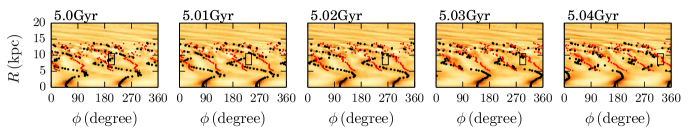
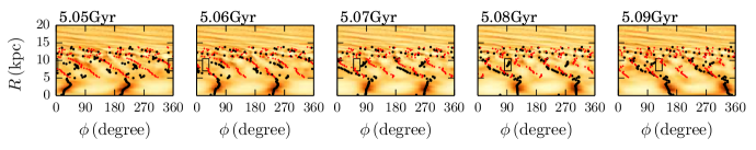
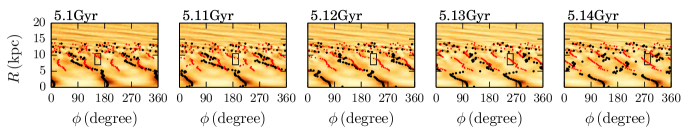
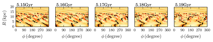
Figure 23: Same as Fig. 17, but for $t=5.00$–$5.19$ Gyr.

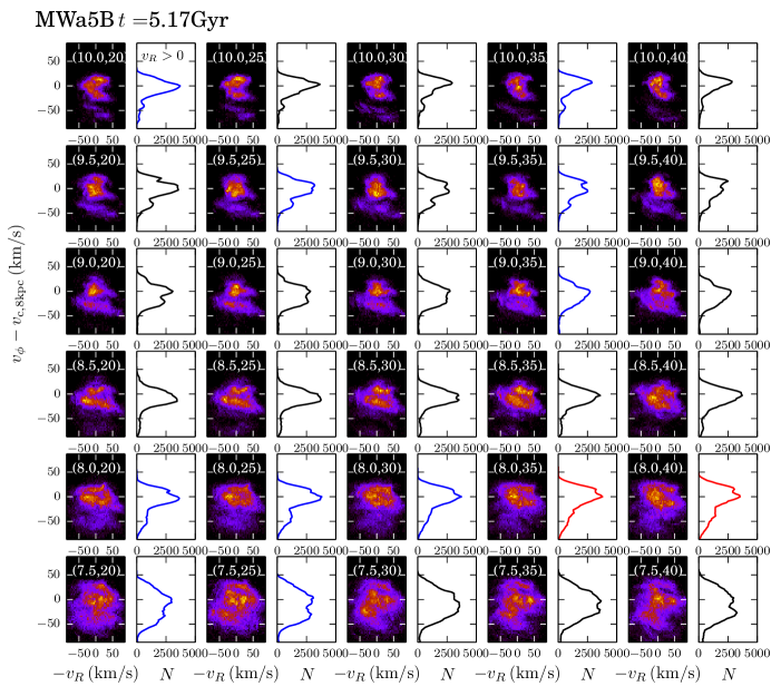
Figure 24: Same as Fig. 18, but for $t=5.17$ Gyr.

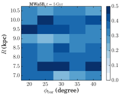
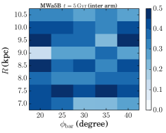
Figure 25: Same as Fig. 20, but for $t=5$ Gyr.

5 Summary

We performed a series of $N$-body simulations of Milky Way models and compared the final products at $t=10$ Gyr with Milky Way Galaxy observations. We found the set of parameters for the initial conditions which are important to reproduce the observed Milky Way galaxy. The stellar disc in our best-fitting model has a mass of $M_{\rm d}\sim 3.7\times 10^{10}M_{\odot}$ and a central velocity dispersion of $\sigma_{R0}\sim 90$ km s^-1. We configured the initial $Q$ value to be 1.2 and the initial disc scale height was set to 0.2 kpc. For the bulge, the initial bulge characteristic velocity of $\sigma_{\rm b}\sim 300$ km s^-1 and bulge scale length of 1 kpc. The bulge mass is not a critical parameter, but if we assume a Hernquist model with the above scale length and velocity we get $M_{\rm b}=3$–$5\times 10^{9}M_{\odot}$. The mass ratio of the bulge-to-disc for the best fitting model is $\sim 0.06$–0.15, which is somewhat higher than previous results, which found that the bulge mass should be less than 8 % of the disc mass in order to reproduce the observed bulge kinematics (Shen et al., 2010).

In our simulations, the angular momentum of the halo is one of the most crucial parameters for reproducing the bar of the Milky Way. The best match with the Milky Way is obtained for a spin parameter of $\lambda\sim 0.06$, which is larger than the mean spin-parameters measured for Milky-Way size dark matter halos of cosmological $N$-body simulations, $\lambda=0.03$–0.04 (Bett et al., 2007), but consistent with the estimated value for short-barred galaxies in SDSS DR7 (Cervantes-Sodi et al., 2013). Without an initial halo spin, we find that the bar that develops is too long and it rotates too slow compared to the bar in the Milky Way.

We also find that the final state of the galactic disc is sensitive to the fraction of disc mass to the total mass of the galaxy ($f_{\rm d}$) in the initial conditions. This parameter controls the bar instability in the sense that a larger value of $f_{\rm d}$ causes the bar to form earlier (Fujii et al., 2018). This parameter correlates with the radial velocity dispersion of the disc at $R=8$ kpc but anti-correlates with the total surface density ($K_{z}/s\pi G$) at $R=8$ kpc. Comparing the bulge kinematics with observations would suggest a larger value of $f_{\rm d}$ when we fix the disc mass and halo spin parameters. Based on these results our models suggest that $f_{\rm d}\sim 0.45$ is preferable for modelling the Milky Way galaxy.

The pattern speed of the bar for our best matching models at an age of $t=10$ Gyr is 40–45 km s^-1 kpc^-1. This is similar to the velocity of a ‘slow’ bar-model in which the Sun is located between the co-rotation and outer Lindblad resonance radii (Pérez-Villegas et al., 2017). Except for the halo spin, the pattern speed of the bar also depends on $f_{\rm d}$. As $f_{\rm d}$ becomes smaller, the pattern speed at $t=10$ Gyr becomes faster. For $f_{\rm d}\sim 0.45$, the expected pattern speed is 40–50 km s^-1. In addition, we did not see any model in which the bar’s pattern speed was faster than $52$ km s^-1 at $t=10$ Gyr.

Based on the “observations” of our best-fitting models, we confirm that we observe the inner-bar structure due to the projection effect and the existence of the bulge (Gerhard & Martinez-Valpuesta, 2012).

The velocity distribution in the solar neighbourhood experiences large changes on a time scale of 20–30 Myr. In at most 50 % of the snapshots, we observed a velocity structure similar to the Hercules stream. The radius at which we most frequently see the Hercules-like stream is slightly further out than the outer Lindblad resonance. If we assume that the Sun is located in an inter-arm region, then the frequency is at most $\sim 50$ %. These variations over time are the result of the complicated interactions between the spiral and bar structure as seen in $N$-body simulations of galactic discs (e.g., Quillen et al., 2011; Baba, 2015). It is thus difficult to give an estimate of the entire galactic disc structure based only on the phase-space distribution of solar neighbourhood stars. Data covering a larger region would be required to make a more precise estimate of the Milky-Way Galaxy structure.

Appendix A Model parameters for all models

We summarize the parameters for the initial conditions and final outcome for all models except for the models shown in the main text. We summarize the parameter sets for GalacICS in Table 5 and the resulting mass and radius of the initial conditions and the number of particles in Table 6. Table 7 contains the disc properties such as velocity dispersion, surface density, the pattern speed of the bar, and the resulting resonance radii at 10 Gyr. In Table 8 we summarize the $\chi^{2}$ value for all models.

Table 5: Model parameters

	Halo				Disc				Bulge
Model	$a_{\rm h}$	$\sigma_{\rm h}$	$\epsilon_{\rm h}$	$\alpha_{\rm h}$	$M_{\rm d}$	$R_{\rm d}$	$z_{\rm d}$	$\sigma_{\rm R0}$	$a_{\rm b}$	$\sigma_{\rm b}$	$\epsilon_{\rm b}$
	(kpc)	($\mathrm{km\ s^{-1}}\,$)			$(10^{10}M_{\odot})$	(kpc)	(kpc)	($\mathrm{km\ s^{-1}}\,$)	(kpc)	$(\mathrm{km\ s^{-1}}\,)$
0	12.5	400	0.8	0.8	4.1	2.6	0.3	94	0.73	333	0.95
1	10.0	400	0.85	0.7	3.1	2.6	0.3	70	0.75	300	0.99
2	12.	409	0.8	0.8	4.1	2.6	0.2	91	0.75	300	0.95
3	10.0	400	0.85	0.8	3.1	2.6	0.3	70	0.75	300	0.99
4	10.0	400	0.85	0.8	3.1	2.6	0.3	70	0.75	300	0.99
5	12.	409	0.8	0.8	3.61	2.6	0.2	83	0.75	300	0.95
6	12.	390	0.8	0.8	4.1	2.6	0.2	90	1.2	280	0.95
7	12.	430	0.8	0.8	4.1	2.6	0.2	91	0.4	300	0.95
8	14.	420	0.82	0.8	3.61	2.6	0.2	85	0.78	280	0.95
9	22.	500	0.7	0.8	3.61	2.6	0.2	90	0.78	280	0.95
10	12.	450	0.8	0.8	4.1	2.6	0.2	91	0.4	330	0.8
11	12.	450	0.8	0.7	4.1	2.6	0.2	91	0.4	330	0.8
12	10.	440	0.85	0.6	4.1	2.6	0.2	87	0.2	400	0.8
13	10.	440	0.85	0.8	4.1	2.6	0.2	87	0.2	400	0.8
14	10.	440	0.85	0.8	4.1	2.6	0.2	87	0.2	400	0.8
15	10.0	440	0.85	0.6	3.61	2.6	0.2	74	0.75	300	0.99
16	10.0	440	0.85	0.7	3.61	2.6	0.2	74	0.75	300	0.99
17	10.0	440	0.85	0.7	3.61	2.6	0.2	80	0.75	300	0.99
18	10.0	440	0.85	0.8	3.61	2.6	0.2	74	0.75	300	0.99
19	10.0	440	0.85	0.65	3.61	2.6	0.3	74	0.75	300	0.99
20	12.0	500	0.8	0.65	3.84	2.6	0.3	75	0.75	300	0.95
21	12.0	500	0.8	0.8	3.84	2.6	0.3	75	0.75	300	0.95
22	10.0	440	0.85	0.8	3.61	2.4	0.3	80	0.75	300	0.99
23	10.0	400	0.85	0.8	3.61	2.3	0.3	85	0.75	330	0.99
24	10.0	440	0.85	0.8	3.61	2.3	0.3	85	0.75	270	0.99
25	12.0	430	0.85	0.8	4.1	3.0	0.2	76	0.75	300	0.99
26	18.0	530	0.75	0.8	4.1	3.0	0.2	75	0.75	300	0.99
27	12.0	440	0.82	0.8	4.05	3.0	0.2	76	0.7	350	0.99
28	18.0	550	0.75	0.8	4.1	3.0	0.2	75	0.75	360	0.99
29	12.0	480	0.82	0.8	3.91	2.8	0.2	76	0.6	365	0.99
30	12.	450	0.8	0.8	4.08	2.6	0.2	88	0.4	350	0.8
31	12.	450	0.8	0.8	4.08	2.6	0.2	91	0.4	350	0.8
32	12.	450	0.8	0.8	3.89	2.6	0.2	85	0.4	370	0.8
33	12.	450	0.8	0.8	3.89	2.6	0.2	92	0.4	370	0.8
34	12.	450	0.8	0.8	4.01	2.6	0.2	87	0.4	360	0.8
35	12.	450	0.8	0.8	4.01	2.6	0.2	94	0.4	360	0.8
36	12.	459	0.8	0.8	3.91	2.6	0.2	86	0.4	400	0.8
37	12.	459	0.8	0.8	3.91	2.6	0.2	92	0.4	400	0.8
38	12.	459	0.8	0.8	3.91	2.6	0.2	92	0.4	400	0.8
39	12.	400	0.8	0.8	3.96	3.2	0.2	72	0.9	300	0.97
40	12.	400	0.8	0.8	3.96	2.9	0.2	80	0.9	300	0.8
41	12.	400	0.8	0.8	3.59	2.2	0.2	96	0.9	300	0.97
42	12.	400	0.8	0.8	3.59	2.6	0.2	82	0.9	300	0.97
43	12.	400	0.8	0.9	3.59	2.2	0.2	96	0.9	300	0.97
44	12.	400	0.8	0.9	3.59	2.2	0.2	105	0.9	300	0.97
45	12.	400	0.8	0.9	3.59	2.6	0.2	89	0.9	300	0.97
46	12.	400	0.8	0.8	3.59	2.4	0.2	82	0.9	300	0.97
47	12.	400	0.8	0.9	3.59	2.4	0.2	82	0.9	300	0.97
48	12.	400	0.8	0.8	3.59	2.4	0.2	82	0.9	300	0.97
49	10.	440	0.85	0.8	3.61	2.3	0.2	85	0.75	330	0.99
50	10.	420	0.85	0.8	3.61	2.3	0.2	88	0.75	330	0.99
51	10.	440	0.85	0.8	3.61	2.3	0.2	92	0.75	340	0.99

Table 6: Mass, radius, and the number of particles

Model	$M_{\rm d}$	$M_{\rm b}$	$M_{\rm h}$	$M_{\rm b}/M_{\rm d}$	$R_{\rm d,t}$	$r_{\rm b,t}$	$r_{\rm h,t}$	$Q_{0}$	$N_{\rm d}$	$N_{\rm b}$	$N_{\rm h}$	$f_{\rm d}$
	($10^{10}M_{\odot}$)	($10^{10}M_{\odot}$)	($10^{10}M_{\odot}$)		(kpc)	(kpc)	(kpc)
0	4.19	0.646	90.7	0.15	31.6	3.3	223.0	1.2	8.3M	1.3M	179M	0.514
1	3.22	0.491	74.6	0.15	31.6	3.29	246.0	1.2	8.3M	1.3M	192M	0.396
2	4.19	0.444	83.6	0.11	31.6	2.89	223.0	1.2	8.3M	0.9M	164M	0.496
3	3.2	0.472	74.8	0.15	31.6	3.28	245.0	1.2	8.3M	1.3M	192M	0.405
4	3.2	0.472	74.8	0.15	31.6	3.28	245.0	1.2	8.3M	1.3M	192M	0.405
5	3.7	0.469	83.2	0.13	31.6	3.03	219.0	1.2	8.3M	0.7M	159M	0.473
6	4.2	0.366	73.1	0.09	31.6	3.13	234.0	1.2	8.3M	0.8M	162M	0.478
7	4.17	0.348	92.0	0.08	31.6	2.25	219.0	1.2	8.3M	0.7M	151M	0.521
8	3.67	0.401	105.8	0.11	31.4	2.99	280.0	1.2	8.3M	0.6M	169M	0.523
9	3.66	0.436	154.4	0.12	31.4	3.25	244.0	1.2	8.3M	1.0M	349M	0.588
10	4.18	0.35	100.7	0.08	31.6	1.63	209.0	1.2	8.3M	0.7M	151M	0.492
11	4.18	0.35	100.7	0.08	31.6	1.63	209.0	1.2	8.3M	0.7M	151M	0.492
12	4.18	0.325	105.0	0.08	31.6	1.13	209.0	1.2	8.3M	0.7M	199M	0.507
13	4.18	0.325	105.0	0.08	31.6	1.13	209.0	1.2	8.3M	0.7M	199M	0.507
14	4.18	0.325	105.0	0.08	31.6	1.13	209.0	1.2	8.3M	0.7M	199M	0.507
15	3.72	0.427	86.4	0.11	31.6	2.95	257.0	1.2	8.3M	1.0M	192M	0.393
16	3.72	0.427	86.4	0.11	31.6	2.95	257.0	1.2	8.3M	1.0M	192M	0.393
17	3.72	0.427	86.4	0.11	31.6	2.95	257.0	1.2	8.3M	1.0M	192M	0.393
18	3.72	0.427	86.4	0.11	31.6	2.95	257.0	1.2	8.3M	1.0M	192M	0.393
19	3.75	0.446	86.1	0.12	31.6	2.96	259.0	1.2	8.3M	1.0M	192M	0.393
20	3.98	0.447	109.9	0.11	31.6	2.72	227.0	1.2	8.3M	1.0M	192M	0.386
21	3.98	0.447	109.9	0.11	31.6	2.72	227.0	1.2	8.3M	1.0M	192M	0.386
22	3.74	0.412	88.3	0.11	31.6	2.75	256.0	1.2	8.3M	0.9M	197M	0.42
23	3.74	0.56	92.2	0.15	31.6	3.11	242.0	1.2	8.3M	0.9M	197M	0.429
24	3.71	0.289	85.4	0.08	31.6	2.41	272.0	1.2	8.3M	0.6M	190M	0.421
25	4.2	0.488	101.7	0.12	31.6	3.39	299.0	1.2	8.3M	0.9M	197M	0.421
26	4.19	0.526	159.4	0.13	31.6	3.64	252.0	1.2	8.3M	0.9M	197M	0.438
27	4.17	0.756	105.2	0.18	31.6	3.98	234.0	1.2	8.3M	1.5M	209M	0.428
28	4.2	0.889	185.2	0.21	31.6	4.44	242.0	1.2	8.3M	1.0M	314M	0.44
29	4.03	0.762	123.2	0.19	31.6	3.7	229.0	1.2	8.3M	1.5M	209M	0.423
30	4.16	0.406	104.4	0.1	31.6	1.69	204.0	1.2	8.3M	0.8M	208M	0.499
31	4.16	0.406	104.4	0.1	31.6	1.69	204.0	1.2	8.3M	0.8M	208M	0.499
32	3.97	0.469	108.3	0.12	31.6	1.76	199.0	1.2	8.3M	1.0M	226M	0.497
33	3.97	0.469	108.3	0.12	31.6	1.76	199.0	1.2	8.3M	1.0M	226M	0.497
34	4.09	0.436	106.4	0.11	31.6	1.73	202.0	1.2	8.3M	0.9M	216M	0.499
35	4.09	0.436	106.4	0.11	31.6	1.73	202.0	1.2	8.3M	0.9M	216M	0.499
36	4.0	0.564	118.0	0.14	31.6	1.83	195.0	1.2	8.3M	1.2M	245M	0.497
37	4.0	0.564	118.0	0.14	31.6	1.83	195.0	1.2	8.3M	1.2M	245M	0.497
38	4.0	0.564	118.0	0.14	31.6	1.83	195.0	1.2	8.3M	1.2M	245M	0.497
39	4.22	0.55	76.1	0.13	31.6	3.73	221.0	1.2	8.3M	1.1M	150M	0.412
40	4.27	0.514	77.7	0.12	31.6	3.52	220.0	1.2	8.3M	0.8M	100M	0.447
41	3.66	0.434	82.5	0.12	31.6	3.05	217.0	1.2	8.3M	1.0M	187M	0.525
42	3.68	0.497	79.5	0.13	31.6	3.41	220.0	1.2	8.3M	1.1M	179M	0.467
43	3.66	0.434	82.5	0.12	31.6	3.05	217.0	1.2	8.3M	1.0M	187M	0.525
44	3.66	0.434	82.5	0.12	31.6	3.05	217.0	1.2	8.3M	1.0M	187M	0.525
45	3.68	0.497	79.5	0.13	31.6	3.41	220.0	1.2	8.3M	1.1M	179M	0.467
46	3.67	0.467	80.9	0.13	31.6	3.24	219.0	1.2	8.3M	1.1M	182M	0.495
47	3.67	0.467	80.9	0.13	31.6	3.24	219.0	1.2	8.3M	1.1M	182M	0.495
48	3.67	0.467	80.9	0.13	31.6	3.24	219.0	1.2	8.3M	1.1M	182M	0.495
49	3.71	0.535	92.5	0.14	31.6	3.09	242.0	1.2	8.3M	1.2M	206M	0.44
50	3.71	0.535	92.5	0.14	31.6	3.09	242.0	1.2	8.3M	1.2M	206M	0.44
51	3.71	0.588	94.0	0.16	31.6	3.21	238.0	1.2	8.3M	1.3M	209M	0.441

Table 7: Disc properties for the simulated galaxies at 10 Gyr

Model	$\Sigma_{\rm 8kpc}$	$\sigma_{R,{\rm 8kpc}}$	$\sigma_{z,{\rm 8kpc}}$	$K_{z,{\rm 8kpc}}$	$V_{\rm c,8kpc}$	$\Omega_{\rm b}$	$R_{\rm CR}$	$R_{\rm OLR}$	$R_{\rm ILR}$
	($M_{\odot}\,{\rm kpc}^{-2}$)	(km s-1)	(km s-1)	($2\pi G\,M_{\odot}\,{\rm kpc}^{-2}$)	(km s-1)	(km s-1 kpc-1)	(kpc)	(kpc)	(kpc)
0	53.6	48.9	20.9	69.3	212.9	36.0	5.6	11.2	2.2
1	40.3	28.3	16.1	66.6	226.7	37.9	5.5	10.7	1.7
2	56.3	47.4	17.4	76.6	223.5	41.9	4.8	9.6	1.9
3	41.2	29.3	16.2	65.0	226.6	45.2	4.4	8.8	1.4
4	40.2	28.9	16.0	65.2	226.8	42.5	4.7	9.4	1.5
5	50.6	47.3	16.5	66.8	216.5	40.9	4.7	9.6	1.9
6	48.8	46.9	16.9	72.0	224.8	35.9	6.0	11.0	2.2
7	55.6	46.7	16.7	74.1	220.2	44.9	4.3	8.6	1.7
8	48.8	46.1	16.6	67.0	211.2	39.4	4.8	10.1	2.0
9	48.8	50.7	17.7	60.8	193.0	33.7	5.3	12.0	2.3
10	54.9	43.6	16.6	74.8	233.1	48.8	4.0	8.4	1.6
11	56.2	42.5	16.4	78.0	234.2	41.3	4.8	10.7	1.8
12	58.2	42.3	16.9	78.5	231.4	34.2	6.1	14.0	2.1
13	60.1	43.0	17.2	80.9	231.8	25.7	9.5	19.4	2.3
14	57.8	43.5	17.2	78.8	231.0	44.2	4.4	9.9	1.7
15	46.5	32.1	14.9	77.7	243.8	24.2	10.4	18.5	3.0
16	47.1	30.8	14.4	79.9	248.2	47.0	4.6	9.4	1.4
17	45.9	31.7	14.2	75.3	248.2	39.0	5.9	11.3	1.8
18	46.0	32.5	14.6	79.3	247.1	50.5	4.3	8.7	1.4
19	45.8	28.0	17.0	77.9	249.4	44.7	5.0	9.8	1.4
20	50.6	28.5	17.5	84.2	259.9	45.5	5.0	10.6	1.5
21	50.7	28.6	17.8	82.2	260.0	51.4	4.3	9.1	1.3
22	44.5	30.6	17.1	75.6	250.3	47.5	4.7	9.3	1.4
23	44.9	40.4	18.9	69.2	232.1	42.0	5.1	10.0	1.9
24	42.1	30.6	17.1	74.5	251.1	46.9	4.9	9.2	1.3
25	55.9	41.1	16.5	78.1	229.8	43.3	4.7	9.6	1.7
26	61.0	47.6	18.2	78.9	223.1	40.8	4.8	10.8	1.9
27	56.5	47.6	17.5	76.3	223.4	40.0	5.0	10.3	2.0
28	54.2	52.8	18.9	72.4	217.5	38.5	5.2	12.2	2.2
29	56.6	43.9	17.2	78.4	235.0	44.0	4.7	10.0	1.8
30	58.0	44.6	17.1	75.1	230.6	45.1	4.3	9.4	1.7
31	57.1	45.5	16.9	78.7	231.0	46.2	4.1	9.3	1.6
32	57.9	45.6	17.6	76.2	224.4	22.6	10.7	21.4	2.8
33	55.0	45.3	16.7	76.1	226.5	45.0	4.2	9.1	1.7
34	58.4	45.9	17.5	76.4	228.4	43.6	4.4	9.6	1.8
35	58.4	44.6	17.2	76.0	228.4	43.3	4.5	9.9	1.7
36	58.7	48.6	17.5	75.6	225.5	42.2	4.5	10.0	1.9
37	56.3	47.4	17.0	75.8	226.6	45.1	4.2	8.8	1.7
38	58.3	46.1	17.0	76.1	226.9	41.9	4.6	10.1	1.9
39	53.1	39.2	15.9	73.9	218.2	39.0	5.1	10.6	1.8
40	53.6	42.9	16.2	77.3	224.3	44.5	4.4	9.2	1.7
41	46.8	49.9	16.8	66.0	220.1	41.4	4.8	29.9	2.0
42	48.6	44.1	16.5	68.2	217.4	39.3	5.0	9.9	1.9
43	46.9	50.6	17.5	67.2	220.1	44.1	4.5	8.6	1.9
44	45.7	50.6	16.9	66.2	220.3	44.3	4.6	29.6	1.9
45	49.0	42.2	15.8	71.5	219.0	44.3	4.4	8.5	1.7
46	47.6	49.1	16.8	68.0	217.6	36.2	5.5	10.7	2.2
47	46.5	52.7	17.5	66.9	215.6	41.3	4.8	9.1	2.2
48	48.5	47.9	17.0	69.2	218.1	38.3	5.2	29.8	2.1
49	45.5	36.4	14.8	72.4	247.8	49.6	4.4	8.9	1.6
50	46.3	41.9	15.7	72.5	238.9	47.7	4.5	9.1	1.7
51	45.4	36.4	14.9	76.3	247.5	34.0	7.1	13.4	1.9

Table 8: $\chi^{2}$ for $\Sigma_{\rm 8kpc}$, $\sigma_{R,{\rm 8kpc}}$, $K_{z,{\rm 8kpc}}$, $v_{\rm los}$, and $\sigma_{\rm los}$

Model	${\Sigma_{\rm 8kpc}}$	$\sigma_{R,{\rm 8kpc}}$	$K_{z,{\rm 8kpc}}$	$v_{\rm los}$	$\sigma_{\rm los}$	total
0	3.6	7.8	0.02	2.0	4.3	17.6
1	4.0	1.8	0.5	1.9	3.0	11.3
2	7.4	6.2	1.7	2.3	1.2	18.7
3	3.0	1.3	1.0	3.1	5.4	13.8
4	4.2	1.5	0.9	2.6	4.5	13.7
5	1.0	6.0	0.4	1.9	1.9	11.4
6	0.3	5.7	0.2	2.3	3.1	11.5
7	6.2	5.5	0.7	2.2	1.9	16.5
8	0.3	4.9	0.4	2.2	1.6	9.3
9	0.2	9.8	3.4	2.0	1.1	16.6
10	5.3	3.0	0.9	2.4	3.9	15.5
11	7.2	2.2	2.6	1.9	1.9	15.7
12	10.6	2.2	2.9	2.0	1.4	19.2
13	14.6	2.6	4.8	2.0	2.4	26.4
14	9.8	2.9	3.1	2.0	2.4	20.2
15	0.03	0.3	2.4	2.2	20.3	25.3
16	0.0	0.7	3.9	3.4	4.2	12.2
17	0.1	0.4	1.1	1.8	2.9	6.4
18	0.1	0.3	3.5	3.1	4.8	11.7
19	0.1	2.0	2.5	2.6	5.7	12.9
20	1.1	1.7	8.1	2.4	6.5	19.7
21	1.1	1.7	5.9	3.3	6.9	18.9
22	0.6	0.8	1.2	5.8	3.5	11.9
23	0.4	1.2	0.02	3.0	2.1	6.7
24	2.2	0.8	0.8	6.0	3.5	13.3
25	6.7	1.5	2.6	2.1	2.7	15.6
26	16.6	6.3	3.2	2.1	1.5	29.7
27	7.6	6.4	1.6	1.9	2.4	19.8
28	4.3	12.7	0.2	1.9	6.8	26.0
29	7.9	3.2	2.8	2.0	1.7	17.6
30	10.3	3.7	1.0	2.1	1.8	18.9
31	8.7	4.4	3.0	2.1	2.9	21.1
32	10.1	4.5	1.6	2.1	2.3	20.6
33	5.4	4.2	1.5	2.1	2.3	15.6
34	11.1	4.8	1.7	2.1	1.5	21.1
35	11.0	3.7	1.4	2.1	1.7	20.0
36	11.7	7.4	1.2	2.1	1.1	23.5
37	7.3	6.2	1.4	2.0	1.6	18.5
38	10.8	4.9	1.5	2.4	1.1	20.7
39	3.1	0.7	0.6	1.9	1.7	8.0
40	3.7	2.5	2.2	3.3	3.6	15.2
41	0.01	8.9	0.6	2.1	1.6	13.4
42	0.2	3.3	0.1	2.0	1.4	7.1
43	0.0	9.7	0.3	2.5	1.1	13.6
44	0.2	9.7	0.6	2.7	1.2	14.3
45	0.3	2.1	0.1	2.2	1.3	6.0
46	0.02	7.9	0.2	2.1	2.4	12.6
47	0.03	12.6	0.4	2.1	1.5	16.6
48	0.2	6.7	0.03	1.9	1.8	10.7
49	0.2	0.1	0.2	2.4	2.0	5.0
50	0.1	1.9	0.3	3.5	1.2	7.0
51	0.3	0.1	1.6	2.3	1.5	5.8

Appendix B The effect of the particle resolution

It is known that the number of particles ($N$) affects the results. Dubinski et al. (2009) showed that the bar formation epoch is delayed if the number of particles increases, because a bar develops from particle noise which in turn depends on $N$. In simulations of spiral galaxies, the maximum and final spiral amplitude depends on $N$ because of the same reason (Fujii et al., 2011).

Even if the number of particles increases, the dynamical evolution of galactic discs may change when we use a different random seed to generate the initial conditions (Sellwood & Debattista, 2009). We, therefore, test the convergence of the results by performing multiple simulations for the same Galaxy model. For this model we vary the number of particles and the random seed. The model parameters for this test are summarized in Tables 9 and 10. We use $N\sim 0.8$M, 8M, and 80M particles for the disc. The total number of particles for each model then becomes $\sim 12$M, 120M, and 1.2B, respectively. For each $N$ we use four different random seeds to generate four different realizations.

In Fig. 26, we present the following results (from top to bottom): bulge radial velocity, velocity dispersion, disc scale height, bar length, bar amplitude, and bar pattern speed. From left to right we show the results for $N\sim 12$M, 120M, and 1.2B. In each panel, the results for the four different runs are over-plotted using different colours. For the top two panels, we also show the BRAVA observations (Kunder et al., 2012).

The convergence of the bulge velocity distribution and disc scale height improves as $N$ increases. The length of the bar changes with time and the fluctuation of the bar length, between the different random seeds, becomes larger as $N$ increases. This may be because finer structures, which affect the bar length, appear in the higher resolution simulations. Indeed, the bar repeatedly connects and disconnects with spiral arms (see Figure 23). Evolution over a longer time scale is, however, similar for all $N$ and the different random seeds only have minor influence.

In the fourth row, we can see that the bar formation epoch is delayed, but the final bar amplitude converges as $N$ increases. The initial peak of the bar amplitude fluctuates for different random seeds, but the final amplitude settles down to similar values. In the bottom row, we present the evolution of the pattern speed of the bar. With the lowest resolution, the pattern speed continuously drops, in contrast for the higher resolutions, it settled down at $t\sim 6$ Gyr. In the highest resolution (1.2B), the results look converged, even for the pattern speed oscillation at $t\sim 5$ Gyr.

Based on the results of these tests, we decided to use models with a total number of particle of $\sim 100$M ($\sim 8$M for discs) to find parameters fitting to the Milky Way observations. We performed additional simulations for some of the best-fitting models, with up to 8 billion particles in total.

Table 9: Model parameters

	Halo				Disc				Bulge
Parameters	$a_{\rm h}$	$\sigma_{\rm h}$	$\epsilon_{\rm h}$	$\alpha_{\rm h}$	$M_{\rm d}$	$R_{\rm d}$	$z_{\rm d}$	$\sigma_{\rm R0}$	$a_{\rm b}$	$\sigma_{\rm b}$	$\epsilon_{\rm b}$
	(kpc)	($\mathrm{km\ s^{-1}}\,$)			$(10^{10}M_{\odot})$	(kpc)	(kpc)	($\mathrm{km\ s^{-1}}\,$)	(kpc)	$(\mathrm{km\ s^{-1}}\,)$
MWtest	15.5	320	0.76	0.8	$4.66$	2.6	0.36	117	0.78	255	0.99

Table 10: Mass, radius, and the number of particles

Model	$M_{\rm d}$	$M_{\rm b}$	$M_{\rm h}$	$M_{\rm b}/M_{\rm d}$	$R_{\rm d,t}$	$r_{\rm b,t}$	$r_{\rm h,t}$	$Q_{0}$	$N_{\rm d}$	$N_{\rm b}$	$N_{\rm h}$
	($10^{10}M_{\odot}$)	($10^{10}M_{\odot}$)	($10^{10}M_{\odot}$)		(kpc)	(kpc)	(kpc)
MWtest120M	4.68	0.329	66.6	0.070	31.6	2.95	254	1.2	8.3M	0.57M	120M

The number of particles for models MWtest12M and MWtest1.2B are 0.1 and 10 times that of model MWtest120M, respectively.

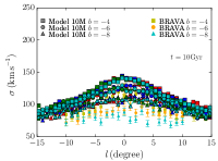
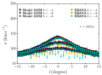
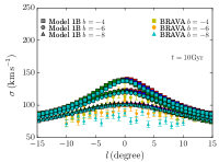
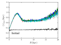
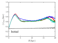
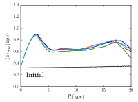
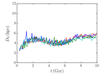
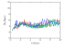
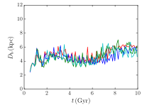
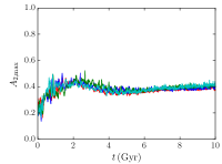
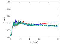
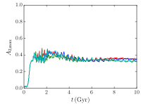
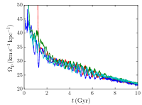
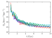
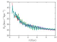
Figure 26: Results for models with different $N$ (12M, 120M, and 1.2B from left to right). From top to bottom the panels show, bulge line-of-sight velocity, bulge velocity dispersion, disc scale height, the evolution of the bar length and the bar amplitude. Colors indicate different random seeds.

Appendix C The Effect of Halo Spin

We investigate the effect of halo spin on the evolution of the disk, and especially the bar structure. In Long et al. (2014), they perform a series of $N$-body simulations changing the initial spin parameter of the halo ($\lambda$). They tested five parameters from 0 to 0.09 and found a sequential change in bar amplitude and pattern speed after 10 Gyr. They also found that the time at which the bar amplitude reaches its maximum is delayed when the halo spin decreases.

Saha & Naab (2013) also performed similar simulations, but for a timescale shorter than the simulations of Long et al. (2014). They, however, also tested a case with a negative initial halo spin and also found a sequential change when negative spin parameters were included.

Here, we perform a series of $N$-body simulations for model MWc where we change the initial halo spin parameter. In addition to models MWc0.5, MWc0.65, and MWc0.8, we performed simulations for the same models but with $\alpha_{\rm h}=0.3$ (model MWc0.3) and 1.0 (model MWc1.0). The initial spin parameters are $\lambda=-0.053$ and $0.14$ for models MWc0.3 and MWc1.0, respectively. Using GalactICS, $\alpha=1.0$ is the maximum spin we can set.

The evolution and the final structures of these models are summarized in Figs. 27 and 28. In Fig. 29, we present the final snapshots of models MWc0.3 and MWc1.0. Model MWc0.3 (negative spin) forms a bar stronger than model MWc0.5 (see Fig. 7). The bar of model MWc1.0 is similar to that of model MWc7B (MWc0.8). In the top panel of Fig. 30, we summarized the time evolution of the bar length for all model MWc variations. The measured bar length is comparable for models MWc0.3 and MWc0.5 and models MWc0.8 and MWc1.0. The evolution of the bar length for model MWc0.65 is similar to that of the high spin models, but the bar becomes slightly longer. We also present the time evolution of the bar pattern speed in the bottom panel of Fig. 30. Although model MWc1.0 has a spin parameter that is larger than used in model MWc0.8, the time evolution and the final pattern speed of the bar is very similar to that of model MWc0.8. For model MWc0.3, which initially has a negative spin parameter, the pattern speed drops most rapidly, and the final pattern speed of the bar is slower than that of model MWc0.5.

We also investigate the evolution of the bar amplitude. We adopt two different definitions for the amplitude. We first measure the average amplitude of the $m=2$ Fourier amplitude (eq. 8) for $R<2.5R_{\rm d}$ ($=6.5$ kpc). This is the same as that used in Long et al. (2014) and ‘Integrated $A_{2}$’ in Saha & Naab (2013). The result is presented in the top panel of Fig. 31. We see features which are also seen in previous studies; for a larger spin model (1) the initial peak amplitude is larger and (2) the peak time is earlier. In Long et al. (2014), the amplitude decreases initially, but increases more than the initial peak for their model without initial halo spin. We see the same evolution behaviour in model MWc0.5. With a negative spin (model MWc0.3), the amplitude decreased and increased again similar as model MWc0.5, but then decreased again after $\sim 5$ Gyr. For positive spin models, the amplitude increased again if the model has a moderate spin (model MWc0.65), but not for the stronger spin models (MWc0.8 and MWc1.0). These results are consistent with previous studies (Long et al., 2014). We also measure the maximum amplitude for amplitudes measured at each galactic radius. This is equivalent with ’Peak of $A_{2}$’ in Saha & Naab (2013). The results are presented in the bottom panel of Fig. 31. The evolution of the peak amplitude is similar to that of the integrated amplitude.

We also measure the final halo spin ($\lambda_{\rm fin}$) and the spin change ($\Delta\lambda=\lambda_{\rm fin}-\lambda_{\rm ini}$). The results are summarized in Table 11. For models with a negative to moderate spin the final spin parameter increased. For the highest spin model (MWc1.0) the final spin parameter was smaller than the initial one.

Thus, the initial halo spin sequencially changes the length and pattern speed of the bar. As the halo spin increases, the bar becomes shorter and the pattern speed increases. This is due to the angular momentum transfer from the bar to the halo (Athanassoula, 2002; Dubinski et al., 2009). This angular momentum transfer seems to saturate if we increase the initial halo spin (maximum spin). This result implies that models with a fixed halo potential would be similar to the maximum spin cases.

Table 11: Spin parameters.

Model	$\alpha_{\rm h}$	$\lambda_{\rm ini}$	$\lambda_{\rm fin}$	$\Delta\lambda$
MWc0.3	0.3	-0.053	-0.047	0.006
MWc0.5	0.5	0.0	0.00050	0.0005
MWc0.65	0.65	0.032	0.036	0.004
MWc0.8	0.8	0.061	0.075	0.014
MWc7B	0.8	0.061	0.072	0.011
MWc1.0	1.0	0.14	0.12	-0.02

$\lambda_{\rm ini}$ and $\lambda_{\rm fin}$ are the initial and final halo spin parameters, and $\Delta\lambda=\lambda_{\rm fin}-\lambda_{\rm ini}$.

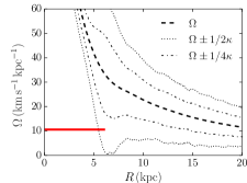
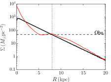
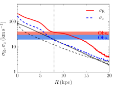
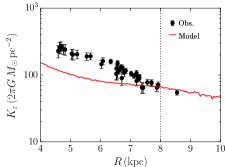
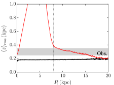
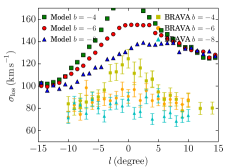
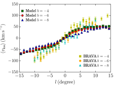
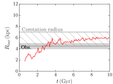
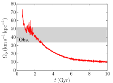
Figure 27: Same as Fig.1, but for model MWc0.3.

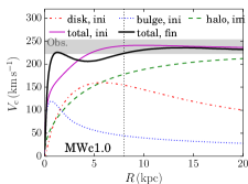
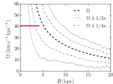
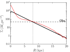
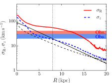
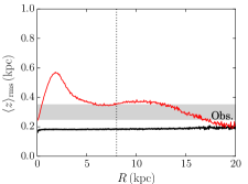
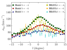
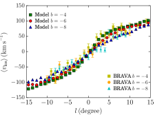
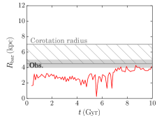
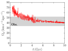
Figure 28: Same as Fig.1, but for model MWc1.0.

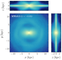
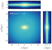
Figure 29: Surface density maps at $t=10$ Gyr for models MWc0.3 and MWc01.0.

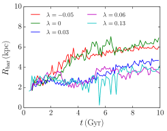
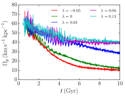
Figure 30: Bar length (top) and pattern speed (bottom) as a function of time for models MWc0.3 ($\lambda=-0.05$), MWc0.5 ($\lambda=0.0$), MWc0.65 ($\lambda=0.03$), MWc0.8 ($\lambda=0.06$), and MWc1.0 ($\lambda=0.13$).

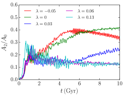
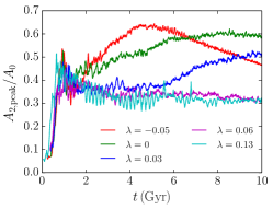
Figure 31: Bar amplitude as a function of time for models MWc0.3 ($\lambda=-0.05$), MWc0.5 ($\lambda=0.0$), MWc0.65 ($\lambda=0.03$), MWc0.8 ($\lambda=0.06$), and MWc1.0 ($\lambda=0.13$). Top panel shows the mean amplitude for $R<0.65$ kpc. Bottom panel shows the peak amplitude measured at each galactic radius.

References

- Abbott et al. (2017) Abbott C. G., Valluri M., Shen J., Debattista V. P., 2017, MNRAS, 470, 1526
- Antoja et al. (2014) Antoja T., et al., 2014, A&A, 563, A60
- Athanassoula (1992) Athanassoula E., 1992, MNRAS, 259, 328
- Athanassoula (2002) Athanassoula E., 2002, ApJ, 569, L83
- Baba (2015) Baba J., 2015, MNRAS, 454, 2954
- Baba et al. (2010) Baba J., Saitoh T. R., Wada K., 2010, PASJ, 62, 1413
- Bédorf et al. (2012) Bédorf J., Gaburov E., Portegies Zwart S., 2012, Journal of Computational Physics, 231, 2825
- Bédorf et al. (2014) Bédorf J., Gaburov E., Fujii M. S., Nitadori K., Ishiyama T., Portegies Zwart S., 2014, in Proceedings of the International Conference for High Performance Computing, Networking, Storage and Analysis, p. 54-65. pp 54–65 (arXiv:1412.0659), doi:10.1109/SC.2014.10OTHER: http://dl.acm.org/citation.cfm?id=2683600
- Bett et al. (2007) Bett P., Eke V., Frenk C. S., Jenkins A., Helly J., Navarro J., 2007, MNRAS, 376, 215
- Binney & Tremaine (2008) Binney J., Tremaine S., 2008, Galactic Dynamics: Second Edition. Princeton University Press
- Bland-Hawthorn & Gerhard (2016) Bland-Hawthorn J., Gerhard O., 2016, ARA&A, 54, 529
- Boekholt & Portegies Zwart (2015) Boekholt T., Portegies Zwart S., 2015, Computational Astrophysics and Cosmology, 2, 2
- Bovy & Rix (2013) Bovy J., Rix H.-W., 2013, ApJ, 779, 115
- Cao et al. (2013) Cao L., Mao S., Nataf D., Rattenbury N. J., Gould A., 2013, MNRAS, 434, 595
- Carlberg (1987) Carlberg R. G., 1987, ApJ, 322, 59
- Cervantes-Sodi et al. (2013) Cervantes-Sodi B., Li C., Park C., Wang L., 2013, ApJ, 775, 19
- Ciambur et al. (2017) Ciambur B. C., Graham A. W., Bland-Hawthorn J., 2017, MNRAS, 471, 3988
- Contopoulos (1980) Contopoulos G., 1980, A&A, 81, 198
- Correa et al. (2015) Correa C. A., Wyithe J. S. B., Schaye J., Duffy A. R., 2015, MNRAS, 452, 1217
- Dehnen (1998) Dehnen W., 1998, AJ, 115, 2384
- Dehnen (2000) Dehnen W., 2000, AJ, 119, 800
- Dubinski et al. (2009) Dubinski J., Berentzen I., Shlosman I., 2009, ApJ, 697, 293
- Francis & Anderson (2009) Francis C., Anderson E., 2009, New A, 14, 615
- Fujii et al. (2011) Fujii M. S., Baba J., Saitoh T. R., Makino J., Kokubo E., Wada K., 2011, ApJ, 730, 109
- Fujii et al. (2018) Fujii M. S., Bédorf J., Baba J., Portegies Zwart S., 2018, MNRAS, 477, 1451
- Fux (1997) Fux R., 1997, A&A, 327, 983
- Gaia Collaboration et al. (2016) Gaia Collaboration et al., 2016, A&A, 595, A1
- Gaia Collaboration et al. (2018) Gaia Collaboration Brown A. G. A., Vallenari A., Prusti T., de Bruijne J. H. J., Babusiaux C., Bailer-Jones C. A. L., 2018, preprint, (arXiv:1804.09365)
- Gardner et al. (2014) Gardner E., Debattista V. P., Robin A. C., Vásquez S., Zoccali M., 2014, MNRAS, 438, 3275
- Gerhard & Martinez-Valpuesta (2012) Gerhard O., Martinez-Valpuesta I., 2012, ApJ, 744, L8
- Gonzalez et al. (2011) Gonzalez O. A., Rejkuba M., Minniti D., Zoccali M., Valenti E., Saito R. K., 2011, A&A, 534, L14
- Hattori et al. (2018) Hattori K., Gouda N., Yano T., Sakai N., Tagawa H., Baba J., Kumamoto J., 2018, preprint, (arXiv:1804.01920)
- Hernquist (1990) Hernquist L., 1990, ApJ, 356, 359
- Howard et al. (2008) Howard C. D., Rich R. M., Reitzel D. B., Koch A., De Propris R., Zhao H., 2008, ApJ, 688, 1060
- Huang et al. (2016) Huang Y., et al., 2016, MNRAS, 463, 2623
- Hunt & Bovy (2018) Hunt J. A. S., Bovy J., 2018, MNRAS, 477, 3945
- Hunt et al. (2018a) Hunt J. A. S., Hong J., Bovy J., Kawata D., Grand R. J. J., 2018a, MNRAS,
- Hunt et al. (2018b) Hunt J. A. S., et al., 2018b, MNRAS, 474, 95
- Jenkins & Binney (1990) Jenkins A., Binney J., 1990, MNRAS, 245, 305
- Klypin et al. (2002) Klypin A., Zhao H., Somerville R. S., 2002, ApJ, 573, 597
- Kuijken & Dubinski (1995) Kuijken K., Dubinski J., 1995, MNRAS, 277, 1341
- Kuijken & Gilmore (1991) Kuijken K., Gilmore G., 1991, ApJ, 367, L9
- Kunder et al. (2012) Kunder A., et al., 2012, AJ, 143, 57
- Long et al. (2014) Long S., Shlosman I., Heller C., 2014, ApJ, 783, L18
- López-Corredoira et al. (2005) López-Corredoira M., Cabrera-Lavers A., Gerhard O. E., 2005, A&A, 439, 107
- McKee et al. (2015) McKee C. F., Parravano A., Hollenbach D. J., 2015, ApJ, 814, 13
- McMillan (2017) McMillan P. J., 2017, MNRAS, 465, 76
- Monari et al. (2017) Monari G., Kawata D., Hunt J. A. S., Famaey B., 2017, MNRAS, 466, L113
- Navarro et al. (1997) Navarro J. F., Frenk C. S., White S. D. M., 1997, ApJ, 490, 493
- Okamoto et al. (2015) Okamoto T., Isoe M., Habe A., 2015, PASJ, 67, 63
- Peebles (1969) Peebles P. J. E., 1969, ApJ, 155, 393
- Peebles (1971) Peebles P. J. E., 1971, A&A, 11, 377
- Pelupessy et al. (2013) Pelupessy F. I., van Elteren A., de Vries N., McMillan S. L. W., Drost N., Portegies Zwart S. F., 2013, A&A, 557, A84
- Pérez-Villegas et al. (2017) Pérez-Villegas A., Portail M., Wegg C., Gerhard O., 2017, ApJ, 840, L2
- Portegies Zwart & Boekholt (2018) Portegies Zwart S. F., Boekholt T. C., 2018, Communications in Nonlinear Science and Numerical Simulation, 61, 160
- Portegies Zwart & McMillan (2018) Portegies Zwart S., McMillan S., 2018, Astrophysical Recipes: the Art of AMUSE. AAS IOP Astronomy
- Portegies Zwart et al. (2013) Portegies Zwart S., McMillan S. L. W., van Elteren E., Pelupessy I., de Vries N., 2013, Computer Physics Communications, 183, 456
- Quillen et al. (2011) Quillen A. C., Dougherty J., Bagley M. B., Minchev I., Comparetta J., 2011, MNRAS, 417, 762
- Quillen et al. (2018) Quillen A. C., et al., 2018, MNRAS, 478, 228
- Reid et al. (2014) Reid M. J., et al., 2014, ApJ, 783, 130
- Saha & Naab (2013) Saha K., Naab T., 2013, MNRAS, 434, 1287
- Sellwood & Debattista (2009) Sellwood J. A., Debattista V. P., 2009, MNRAS, 398, 1279
- Sellwood & Sparke (1988) Sellwood J. A., Sparke L. S., 1988, MNRAS, 231, 25P
- Shen et al. (2010) Shen J., Rich R. M., Kormendy J., Howard C. D., De Propris R., Kunder A., 2010, ApJ, 720, L72
- Sofue (2012) Sofue Y., 2012, PASJ, 64, 75
- Toomre (1964) Toomre A., 1964, ApJ, 139, 1217
- Tremaine et al. (2002) Tremaine S., et al., 2002, ApJ, 574, 740
- Vallée (2017) Vallée J. P., 2017, New A Rev., 79, 49
- Wegg & Gerhard (2013) Wegg C., Gerhard O., 2013, MNRAS, 435, 1874
- Wegg et al. (2015) Wegg C., Gerhard O., Portail M., 2015, MNRAS, 450, 4050
- Widrow & Dubinski (2005) Widrow L. M., Dubinski J., 2005, ApJ, 631, 838
- Widrow et al. (2008) Widrow L. M., Pym B., Dubinski J., 2008, ApJ, 679, 1239
- Zoccali & Valenti (2016) Zoccali M., Valenti E., 2016, PASA, 33, e025