An extension of the Eshelby conjecture to domains of general shape in anti-plane elasticity

Abstract

According to the Eshelby conjecture, an ellipse or ellipsoid is the only shape that induces an interior uniform strain under a uniform far-field loading. We extend the Eshelby conjecture to domains of general shape for anti-plane elasticity. Specifically, we show that for each positive integer $N$, an inclusion induces an interior uniform strain under a polynomial loading of degree $N$ if and only if the exterior conformal map of the inclusion is a Laurent series of degree $N$. Furthermore, for the isotropic case, we characterize the shape of an inclusion by only using the first-degree polynomial loading and explicitly solve the interior potential of the inclusion in terms of the Grunsky coefficients.

AMS subject classifications. 30C35; 35J05; 45P05

Key words. Eshelby conjecture, Anti-plane elasticity, Faber polynomial

1 Introduction

We consider the field perturbation due to the presence of an inclusion in a homogeneous background. An inclusion whose material parameter is different from that of the background brings a field perturbation to its exterior and interior. The resulting perturbation depends on the shape of the inclusion as well as the material parameter, and certain shapes admit extremal properties. In 1957, Eshelby discovered that an ellipsoid embedded in an infinite elastic medium induces a uniform interior strain for uniform loadings [14]. Then, he made the following conjecture, which is known as the Eshelby conjecture, in [15]: “Among closed surfaces, the ellipsoid alone has this convenient property.” In this study, we extend this uniformity property to inclusions of general shape by using higher-order loadings, for anti-plane elasticity.

The Eshelby conjecture was proven by Sendeckyj [44] for two dimensions and by Ru and Schiavone [43] for anti-plane elasticity. To prove the conjecture, Ru and Schiavone [43] and Sendeckyj [44] used complex analytic function theory. Kang and Milton [26] provided an alternative proof using the hodograph transformation. Various non-ellipsoidal shapes were shown not to satisfy the Eshelby uniformity property in three dimensions. For example, Rodin [40] considered polyhedral inclusions, Markenscoff [35] inclusions with a planar piece on their boundary, and Lubarda and Markenscoff [34] non-convex inclusions. Markenscoff obtained that the space of domains satisfying the Eshelby uniformity property forms a nine-dimensional manifold [36]. Finally, the conjecture for three dimensions was proven by Kang and Milton [26] and Liu [33] in relation to the Newtonian potential. We recommend that readers refer to the review article by Kang [23] to determine more relations of the Eshelby conjecture with the Pólya-Szegö conjecture and the Newtonian potential problem.

Shapes other than ellipses or ellipsoids can also satisfy the uniformity property with a modified condition from the Eshelby conjecture. Finding Eshelby inclusions, which denote inclusions undergoing a uniform eigenstress with either a far-field loading or a modified condition, has practical applications for designing composites that result in small variances in internal stresses. A multiply connected inclusion can satisfy the uniformity property [8, 24, 30, 33], and so can a non-elliptical simply connected inclusion on a bounded domain containing the inclusion with some boundary condition [4, 25, 32]. Kang et al. constructed Eshelby inclusions with two disjoint components in two dimensions using the hodograph transformation technique [24], and Liu designed multiply connected ones in two and three dimensions with a variational approach [33]. Ru derived analytic solutions for Eshelby inclusions of arbitrary shape in a plane or half-plane in terms of some complex analytic functions [41, 42]. Kang et al. [25] and Bardsley et al. [4] designed various Eshelby inclusions embedded in a bounded domain using the hodograph transformation technique. Wang et al. found Eshelby inclusions of arbitrary shape with the traction-free condition on a curvilinear boundary [48]. Lim and Milton found Eshelby inclusions of arbitrary shape embedded in a bounded domain using the conformal mapping technique [32]; see also [37, 49]. We refer to the works by Vigdergauz [47] and by Grabovsky and Kohn [18] for Vigdergauz microstructures, which are inclusions with the uniformity property with periodic boundary conditions. Furthermore, analytic and numerical methods to compute the elastic tensor (often called the Eshelby tensor field) for inclusions of various shapes have been developed [7, 17, 19, 20, 31, 38, 50]. Additionally, note that the uniformity property can play a significant role in imaging problems. For example, a location search algorithm for a ball-shaped anomaly was developed by using the fact that the induced electric field is uniform inside a ball [29].

In this paper, we investigate the shape of an inclusion which undergoes a uniform eigenstress with a far-field polynomial loading of given degree. If an inclusion has a general shape such that the exterior conformal mapping corresponding to this inclusion is a Laurent series with terms of order $\leq-2$, then the resulting solution due to a uniform loading contains some terms of degree $\geq 2$ in the interior of the inclusion (see, for example, [3]). Instead, the stress field is uniform for a polynomial loading as shown in [44] for the plane elastostatic problem; one can observe this case from [43] for anti-plane elasticity. In fact, the Eshelby conjecture can be generalized to characterize the shape of which an inclusion undergoes a uniform eigenstress with a polynomial loading of given degree (for details, see Theorem 2.1). To the best of our knowledge, there have been no reports on extending the Eshelby conjecture to provide a characterization scheme for inclusions of general shape. Furthermore, we explicitly find the polynomial loading which induces a uniform strain inside the inclusion in a simple form by using the Faber polynomials. For the isotropic case, we also explicitly express the field perturbation using the Grunsky coefficients and find a characterization scheme for the shape of the inclusion by using only a first-degree polynomial loading.

Our analysis is based on the geometric series expansions of the layer potential operators, recently developed by Jung and Lim [21]. This method provides a new powerful scheme to address the conductivity inclusion problems. We emphasize that with the density basis functions constructed in [21], the interface problem of anti-plane elasticity in the presence of a simply connected inclusion can be reformulated to a matrix problem. This matrix formulation gives us explicit relations between the exterior conformal mapping of the inclusion and the applied far-field loading, given that the resulting field is uniform inside the inclusion. It is worth remarking that by using this solution method, one can construct neutral inclusions of multi-layer structure [10] and derive an asymptotic formula to approximate the shape of an inclusion by considering the inclusion as a perturbation of its equivalent ellipse [9]. The decay property of eigenvalues of the Neumann-Poincaré operator was also obtained [22].

The remainder of this paper is organized as follows. We state the main results in section 2. Section 3 provides the boundary integral formulation for the conductivity transmission problem and the geometric series expansions for the layer potential operators. In section 4, we derive essential relations for the density function in the boundary integral formulation. The proofs of the main results are presented in section 5. We finish with the conclusion in section 6.

2 Main results

Let $\Omega$ be a simply connected, bounded planar domain with $C^{1,\alpha}$ boundary for some $\alpha\in(0,1)$. We assume $\Omega$ has a constant, possibly anisotropic, conductivity $\bm{\sigma}$. We consider the transmission problem

$$\begin{cases}\displaystyle\nabla\cdot\left(\bm{\sigma}\chi(\Omega)+\bm{I}\chi(\mathbb{R}^{2}\setminus\overline{\Omega})\right)\nabla u=0\quad&\mbox{in }\mathbb{R}^{2}\setminus\partial\Omega,\\ \displaystyle u(x)-H(x)=O({|x|^{-1}})\quad&\mbox{as }|x|\to\infty\end{cases}$$ (2.1)

for a given far-field loading $H$, which is an entire harmonic function. The symbol $\chi$ indicates the characteristic function, and $\bm{I}$ is the $2\times 2$ identity matrix. We assume $\bm{I}-\bm{\sigma}$ is either positive or negative definite and, hence, (2.1) is solvable (see [13]). One can easily show that $u$ satisfies

$$u\big{|}^{+}=u\big{|}^{-},\quad\nu\cdot\nabla u\big{|}^{+}=\nu\cdot\bm{\sigma}\nabla u\big{|}^{-}\quad\mbox{on }\partial\Omega,$$ (2.2)

where $\nu$ denotes the outward unit normal vector to $\partial\Omega$, and the symbols $+$ and $-$ indicate the limit from the exterior and interior of $\Omega$, respectively.

Let us introduce some terminology before stating main results. We identify $x=(x_{1},x_{2})$ in $\mathbb{R}^{2}$ with $z=x_{1}+\mathrm{i}x_{2}$ in $\mathbb{C}$. The symbols $\operatorname{Re}$ and $\operatorname{Im}$ indicate the real and imaginary parts of complex numbers, respectively. From the Riemann mapping theorem, there exists a unique $\gamma>0$ and a conformal mapping $\Psi$ from $\{w\in\mathbb{C}:|w|>\gamma\}$ onto $\mathbb{C}\setminus\overline{\Omega}$ satisfying $\Psi(\infty)=\infty$ and $\Psi^{\prime}(\infty)=1$. This map admits the Laurent series expansion

$$\Psi(w)=w+a_{0}+\frac{a_{1}}{w}+\frac{a_{2}}{w^{2}}+\cdots$$ (2.3)

with complex coefficients $a_{k}$; one can find the derivation in [39, Chapter 1.2]. The exterior conformal mapping $\Psi$ determines the so-called Faber polynomials $F_{m}(z)$, which are monic polynomials of degree $m$ determined by $a_{0},\dots,a_{m-1}$ and form a basis for analytic functions in $\Omega$ [45]. We define a formal infinite series associated with $\Omega$ in terms of Faber polynomials as

$$\mathfrak{F}(z):=\sum_{m=2}^{\infty}\frac{\overline{a_{m}}}{\gamma^{2m}}F_{m}(z).$$

For an ellipse, $a_{m}=0$ for all $m\geq 2$ and the corresponding formal infinite series $\mathfrak{F}(z)$ is the zero function. By generalizing this characterization of an ellipse, we define classes of shape: For each $N\in\mathbb{N}$, we call $\Omega$ a domain of order $\it N$ if

$$\Psi(w)=w+a_{0}+\frac{a_{1}}{w}+\cdots+\frac{a_{N}}{w^{N}}\ (a_{N}\neq 0).$$ (2.4)

We call a disk, as well as ellipses, a domain of order $1$. If $\Omega$ is a domain of order $N\geq 2$, then $\mathfrak{F}(z)$ is a polynomial of degree $N$. On the other hand, if the far-field loading is a real harmonic polynomial of degree $N$, then it can be expressed as

$$H(x)=\frac{1}{2}\sum_{m=0}^{N}\left(\alpha_{m}F_{m}(z)+\overline{\alpha_{m}F_{m}(z)}\right)$$ (2.5)

with some complex coefficients $\alpha_{m}$. Here, $\alpha_{m}=0$ for all $m\geq N+1$.

The main object of this study is to find an equivalent condition for $\Omega$ to induce a uniform strain inside $\Omega$ under a far-field loading of given finite degree. First, we extend the Eshelby conjecture in anti-plane elasticity and characterize domains of higher-order (see Theorem 2.1 below). One can consider this result as an extension of the strong Eshelby conjecture, following the terminology in [26], in the sense that the uniformity property for just one loading implies the shape of the inclusion. The proofs of the main results are provided in section 5.

Theorem 2.1 (Anisotropic case).

Assume that $\Omega$ is a simply connected, bounded planar domain with $C^{1,\alpha}$ boundary for some $\alpha\in(0,1)$ and $\bm{\sigma}$ is possibly anisotropic. For arbitrary $N\in\mathbb{N}$, the followings are equivalent:

• $\Omega$ is a domain of order $N$.

• For some polynomial loading $H$ of degree $N$, the solution $u$ to (2.1) has a uniform strain inside $\Omega$.

Furthermore, we can explicitly find the far-field loading functions that induce the uniformity in terms of Faber polynomials. To state the formula, we need the following $2\times 2$ real matrix

$$\bm{\tau}(t)=(1-2t)\begin{bmatrix}\displaystyle\operatorname{Re}\left\{{\tau_{1}}(t)\right\}&-\operatorname{Im}\left\{{\tau_{2}}(t)\right\}\\[5.69054pt] \displaystyle\operatorname{Im}\left\{{\tau_{1}}(t)\right\}&\leavevmode\nobreak\ \leavevmode\nobreak\ \operatorname{Re}\left\{{\tau_{2}}(t)\right\}\end{bmatrix}$$ (2.6)

with

$${\tau_{1}}(t)=\frac{\dfrac{a_{1}}{\gamma^{2}}+2t}{\left|\dfrac{a_{1}}{\gamma^{2}}\right|^{2}-4t^{2}},\quad{\tau_{2}}(t)=\frac{-\dfrac{a_{1}}{\gamma^{2}}+2t}{\left|\dfrac{a_{1}}{\gamma^{2}}\right|^{2}-4t^{2}}.$$ (2.7)

As is popularly known as the Bieberbach conjecture [5], the coefficient $a_{1}$ of the exterior conformal mapping $\Psi$ satisfies

$$|a_{1}|<\gamma^{2}.$$

Hence, $\bm{\tau}(t)$ is invertible for all $t\in(-\infty,-1/2]\cup(1/2,\infty)$. In particular, $\bm{\tau}(-1/2)$ is invertible.

Theorem 2.2 (Anisotropic case).

Let $\Omega$ be a domain of arbitrary finite order and $\bm{\sigma}$ be possibly anisotropic. For any real constant vector $(e_{1},e_{2})$, $u$ admits the uniform interior strain $\nabla u=(e_{1},e_{2})$ for the polynomial loading $H(x)$ given by

$$H(x)=f_{1}x_{1}+f_{2}x_{2}+c_{1}\operatorname{Re}\big{\{}z+{{\tau_{1}}(-1/2)}\,\mathfrak{F}(z)\big{\}}+c_{2}\operatorname{Im}\big{\{}z-{{\tau_{2}}(-1/2)}\,\mathfrak{F}(z)\big{\}}$$ (2.8)

with

$$\begin{gathered}\begin{bmatrix}\displaystyle f_{1}\\ \displaystyle f_{2}\end{bmatrix}={\bm{\sigma}}\begin{bmatrix}\displaystyle e_{1}\\ \displaystyle e_{2}\end{bmatrix},\quad\begin{bmatrix}\displaystyle c_{1}\\ \displaystyle c_{2}\end{bmatrix}=\bm{\tau}(-1/2)^{-1}(\bm{I}-\bm{\sigma})\begin{bmatrix}\displaystyle e_{1}\\ \displaystyle e_{2}\end{bmatrix}.\end{gathered}$$ (2.9)

In fact, $H$ given by (2.8) are the only far-field loadings of finite degree that induce a uniform strain in $\Omega$.

Interestingly, for a domain of any finite order, the far-field loading that admits a uniform eigenstress is a linear combination of two functions. We also emphasize that the formulations (2.8)–(2.9) depend only on $\mathfrak{F}(z)$ and $\bm{\sigma}$.

If $\bm{\sigma}$ is isotropic, we can also characterize the shape of an inclusion by only using the first-degree polynomial loadings as follows.

Theorem 2.3 (Isotropic case).

Assume $\bm{\sigma}=\sigma\bm{I}$ and set $\lambda=\frac{\sigma+1}{2(\sigma-1)}$. Let $u$ be the solution to (2.1). For arbitrary $N\in\mathbb{N}$, the followings are equivalent:

• $\Omega$ is a domain of order $N$.

• For some polynomial loading $H$ of degree $1$, the function $(\lambda+\frac{1}{2})(u-H)-\mathcal{D}_{\partial\Omega}\left[(u-H)|_{\partial\Omega}\right]$ is a polynomial of degree $N$ in $\Omega$.

Here, $\mathcal{D}_{\partial\Omega}$ denotes the double-layer potential associated with $\Omega$ (see (3.1)).

In addition, we can explicitly express $u$ as a Faber polynomial expansion for a given polynomial loading of arbitrary degree. The expansion coefficients have a matrix form as follows.

Theorem 2.4 (Isotropic case).

Let $\Omega$ be a $C^{1,\alpha}$ domain for some $\alpha\in(0,1)$. Assume $\bm{\sigma}=\sigma\bm{I}$ and set $\lambda=\frac{\sigma+1}{2(\sigma-1)}$. For a polynomial loading $H$ given by (2.5) with arbitrary degree $N$, the solution $u$ to (2.1) can be expanded as

$$u(x)=\frac{1}{2}\sum_{m=0}^{\infty}\left(\beta_{m}F_{m}(z)+\overline{\beta_{m}F_{m}(z)}\right)\quad\mbox{in }{\Omega}$$

with

$$\bm{\beta}=\left(\lambda-\frac{1}{2}\right)\left(\lambda\bm{\alpha}\gamma^{2\mathbb{N}}+\frac{1}{2}\overline{\bm{\alpha}C}\right)\left(\lambda^{2}I-\frac{\gamma^{-2\mathbb{N}}C\gamma^{-2\mathbb{N}}\overline{C}}{4}\right)^{-1}\gamma^{-2\mathbb{N}},$$

where $\bm{\alpha}=(\alpha_{m})_{m=1}^{\infty}$ and $\bm{\beta}=(\beta_{m})_{m=1}^{\infty}$ are infinite row vectors, and $C=(c_{mk})_{m,k=1}^{\infty}$ is a semi-infinite matrix defined by the Grunsky coefficients $c_{mk}$ of $\Omega$ (see (3.7) for the definition), and $\gamma^{-2\mathbb{N}}$ is a semi-infinite diagonal matrix whose $(m,m)$-entry is $\gamma^{-2m}$ for each $m\in\mathbb{N}$.

Figures 2.1–2.2 illustrate the result in Theorem 2.2. In all examples, the potential difference in $u$ between the neighboring level curves is $1/2$. The loading function $H$ is given by (2.8)–(2.9) such that $(f_{1}+c_{1},f_{2}+c_{2})=(0,1)$ in Figure 2.1; $(c_{1},c_{2})=(1,0)$ in the first row of Figure 2.2; $(c_{1},c_{2})=(0,1)$ in the second row of Figure 2.2.

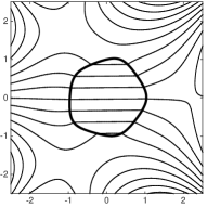
(a) $\sigma=\begin{bmatrix}0.99&0\\ 0&0.2\end{bmatrix}$

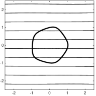
(b) $\sigma=\begin{bmatrix}0.2&0\\ 0&0.99\end{bmatrix}$

Figure 2.1: Anisotropic case. Thin curves are level curves of $u$ and thick curves indicate $\partial\Omega$. The domain $\Omega$ is of order $N=4$, where $\gamma=1$, $a_{1}=0.1\mathrm{i}*s$, $a_{2}=-0.05\mathrm{i}*s$, $a_{3}=0$, and $a_{4}=0.15*s$ with $s=\frac{1}{4}$.

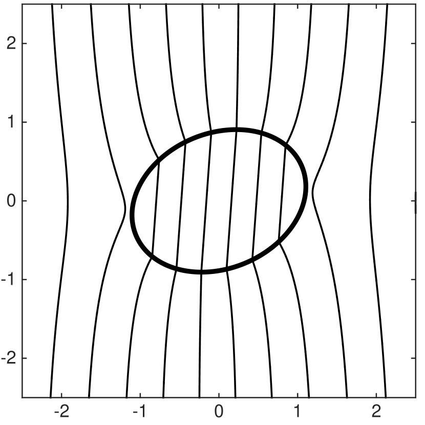
(a) $N=1$

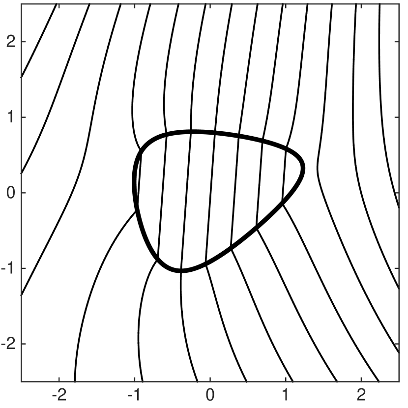
(b) $N=2$

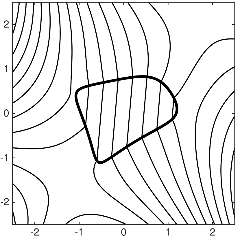
(c) $N=3$

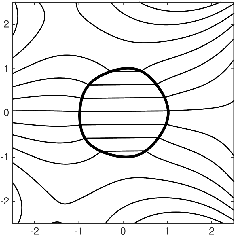
(d) $s=\frac{1}{8}$

(e) $s=\frac{1}{4}$

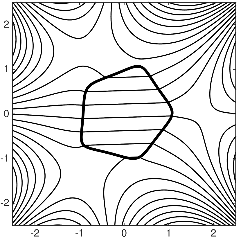
(f) $s=\frac{1}{2}$

Figure 2.2: Isotropic case ($\sigma=0.2$). In the first row, $\Omega$ is a domain of order $N=1,2,3$ given by (2.4), where $\gamma=1$, $a_{1}=0.1+0.1\mathrm{i}$, $a_{2}=0.1+0.1\mathrm{i}$, and $a_{3}=-0.1\mathrm{i}$. In the second row, $\Omega$ is given as in Figure 2.1 with variant $s$; as $\Omega$ more resembles a disk with smaller $s$, the corresponding $H$ has smaller higher-order coefficients.

3 Preliminary

3.1 Boundary integral formulation for the conductivity transmission problem

Let $\Omega$ be a Lipschitz domain in $\mathbb{R}^{2}$. For $\varphi\in L^{2}(\partial\Omega)$, the single- and double-layer potentials are defined as

$$\mathcal{S}_{\partial\Omega}[\varphi](x) =\int_{\partial\Omega}\Gamma(x-y)\varphi(y)\,d\sigma(y),\quad x\in\mathbb{R}^{2},$$

$$\mathcal{D}_{\partial\Omega}[\varphi](x) =\int_{\partial\Omega}\frac{\partial}{\partial\nu_{y}}\Gamma(x-y)\varphi(y)\,d\sigma(y),\quad x\in\mathbb{R}^{2}\setminus\partial\Omega,$$ (3.1)

where $\Gamma$ is the fundamental solution to the Laplacian, i.e., $\Gamma(x)=\frac{1}{2\pi}\ln|x|$, and $\nu_{y}$ denotes the outward unit normal vector to $\partial\Omega$. The single-layer potential has the jump relation

$$\displaystyle\frac{\partial}{\partial\nu}\mathcal{S}_{\partial\Omega}[\varphi]\Big{|}^{\pm} =\left(\pm\frac{1}{2}I+\mathcal{K}^{*}_{\partial\Omega}\right)[\varphi]\quad\mbox{on }\partial\Omega,$$ (3.2)

where $I$ denotes the identity operator on $L^{2}(\partial\Omega)$ and $\mathcal{K}_{\partial\Omega}^{*}$ is the so-called Neumann–Poincaré (NP) operator. The NP operator is the boundary integral operator defined as

$$\displaystyle\mathcal{K}^{*}_{\partial\Omega}[\varphi](x) =\text{p.v.}\,\frac{1}{2\pi}\int_{\partial\Omega}\frac{\left<x-y,\nu_{x}\right>}{|x-y|^{2}}\varphi(y)\,d\sigma(y),$$

where p.v. stands for the Cauchy principal value.

We set $\mathcal{S}_{\partial\Omega}[\varphi](z):=\mathcal{S}_{\partial\Omega}[\varphi](x)$ for $z=x_{1}+\mathrm{i}x_{2}$. Likewise, we define $\mathcal{D}_{\partial\Omega}[\varphi](z)$ and $\mathcal{K}^{*}_{\partial\Omega}[\varphi](z)$.

Isotropic case. When $\bm{\sigma}=\sigma\bm{I}$, $0<\sigma\neq 1<\infty$, the solution $u$ to (2.1) can be expressed as

$$u(x)=H(x)+\mathcal{S}_{\partial\Omega}[\varphi](x)\quad\mbox{in }\mathbb{R}^{2},$$ (3.3)

where $\varphi\in L^{2}_{0}(\partial\Omega)$ (i.e., $\varphi$ is square-integrable and has a zero average value) is given by

$$\varphi=(\lambda I-\mathcal{K}_{\partial\Omega}^{*})^{-1}\left[\nu\cdot\nabla H\right]\quad\mbox{with }\lambda=\frac{\sigma+1}{2(\sigma-1)}.$$ (3.4)

The operator $\mathcal{K}^{*}_{\partial\Omega}$ is bounded on $L^{2}(\partial\Omega)$, and $\lambda I-\mathcal{K}_{\partial\Omega}^{*}$ is invertible on $L^{2}_{0}(\partial\Omega)$ for $|\lambda|\geq 1/2$ [12, 27, 46]. For more properties of the NP operator, we refer the readers to [1, 2, 28] and the references therein.

Anisotropic case. We now assume that $\bm{\sigma}$ is anisotropic. In other words, $\bm{\sigma}$ is a $2\times 2$ positive definite symmetric matrix satisfying that $\bm{I}-\bm{\sigma}$ is either positive or negative definite. For $\psi\in L^{2}(\partial\Omega)$, we define the single-layer potential associated with $\bm{\sigma}$ as

$$\mathcal{S}^{\bm{\sigma}}_{\partial\Omega}[\psi](x)=\int_{\partial\Omega}\Gamma^{\bm{\sigma}}(x-y)\psi(y)\,d\sigma(y)\quad\mbox{in }\mathbb{R}^{2},$$

where

$$\Gamma^{\bm{\sigma}}(x)=\frac{1}{2\pi\sqrt{\mbox{det}(\bm{\sigma})}}\ln\left|\bm{\sigma}^{-\frac{1}{2}}x\right|$$

and $\bm{\sigma}^{-\frac{1}{2}}$ is the inverse of the square root matrix of $\bm{\sigma}$. The solution $u$ to (2.1) with the anisotropic conductivity $\bm{\sigma}$ can be expressed as (see [13])

$$u(x)=\begin{cases}\displaystyle H(x)+\mathcal{S}_{\partial\Omega}[\varphi](x)\quad&\mbox{in }\mathbb{R}^{2}\setminus\overline{\Omega},\\ \displaystyle\mathcal{S}^{\bm{\sigma}}_{\partial\Omega}[\psi](x)\quad&\mbox{in }\Omega,\end{cases}$$ (3.5)

where the density functions $(\psi,\varphi)\in L^{2}(\partial\Omega)\times L^{2}_{0}(\partial\Omega)$ satisfy

$$\begin{cases}\displaystyle\mathcal{S}^{\bm{\sigma}}_{\partial\Omega}[\psi]-\mathcal{S}_{\partial\Omega}[\varphi]=H,\\ \displaystyle\nu\cdot\bm{\sigma}\nabla\mathcal{S}^{\bm{\sigma}}_{\partial\Omega}[\psi]\Big{|}^{-}-\nu\cdot\nabla\mathcal{S}_{\partial\Omega}[\varphi]\Big{|}^{+}=\nu\cdot\nabla H\quad\mbox{on }\partial\Omega.\end{cases}$$

3.2 Geometric series expansions of the layer potential operators

The exterior conformal mapping $\Psi$ associated with $\Omega$ (see (2.3)) uniquely defines the so-called Faber polynomials $F_{m}(z)$ via the generating relation

$$\frac{w\Psi^{\prime}(w)}{\Psi(w)-z}=\sum_{m=0}^{\infty}\frac{F_{m}(z)}{w^{m}}\quad\mbox{for }z\in{\Omega},\ |w|>\gamma.$$ (3.6)

Then, $F_{m}(\Psi(w))$ has only one positive term $w^{m}$, i.e.,

$$F_{m}(\Psi(w))=w^{m}+\sum_{k=1}^{\infty}c_{mk}{w^{-k}},$$ (3.7)

where $c_{mk}$ are called the Grunsky coefficients. The symmetric relation

$$kc_{mk}=mc_{km}$$

holds for all $m,k\in\mathbb{N}$. The concept of Faber polynomials was first introduced by G. Faber [16] and has been one of the essential elements in geometric function theory (see [11]).

Each $F_{m}$ is an $m$-th order monic polynomial uniquely determined by the coefficients $a_{0},a_{1},\cdots,a_{m-1}$ of $\Psi$; a recursive formula to compute the coefficients of Faber polynomials is well known [11, Ch.4]. The first three Faber polynomials are

$$F_{0}(z)=1,\quad F_{1}(z)=z-a_{0},\quad F_{2}(z)=z^{2}-2a_{0}z+(a_{0}^{2}-2a_{1}).$$

From the fact that $F_{1}(z)=z-a_{0}$ and the symmetricity, we have $c_{1k}=a_{k}$ and

$$c_{k1}=kc_{1k}=ka_{k}\quad\mbox{for all }k\in\mathbb{N}.$$ (3.8)

Because $F_{m}(z)$ is a monic polynomial of order $m$ (the highest order term is $z^{m}$), we obtain the following lemma by substituting (2.4) into (3.7).

Lemma 3.1.

Let $\Omega$ be a domain of order $N\geq 2$. Then, $c_{m,Nm}=(a_{N})^{m}\neq 0$ and $c_{mk}=c_{km}=0$ for all $m\in\mathbb{N}$, $k\geq Nm+1$.

We recall that $\Omega$ is assumed to be $C^{1,\alpha}$. The continuous extension of the conformal mapping to the boundary is well known [6]. Furthermore, by the Kellogg-Warschawski theorem [39], $\Psi^{\prime}$ also has continuous extension to the boundary. We define a curvilinear orthogonal coordinates $(\rho,\theta)\in[\rho_{0},\infty)\times[0,2\pi)$ via the relation

$$z=\Psi(e^{\rho+\mathrm{i}\theta})\quad\mbox{for }z\in\mathbb{C}\setminus\Omega.$$ (3.9)

For simplicity, we set $v(\rho,\theta)=v\left(\Psi(e^{\rho+\mathrm{i}\theta})\right)$ for a complex function $v$. The scale factors with respect to $\rho$ and $\theta$ coincide with each other. We denote them by

$$h(\rho,\theta):=\left|\frac{\partial\Psi}{\partial\rho}\right|=\left|\frac{\partial\Psi}{\partial\theta}\right|.$$

On $\partial\Omega$, it then holds that

$$d\sigma(z)=h(\rho_{0},\theta)d\theta$$

and

$$\frac{\partial v}{\partial\nu}\Big{|}_{\partial\Omega}^{+}(z)=\frac{1}{h(\rho,\theta)}\frac{\partial}{\partial\rho}v(\rho,\theta)\Big{|}_{\rho\rightarrow\rho_{0}^{+}}.$$ (3.10)

We denote $\langle\cdot,\cdot\rangle$ as the inner product in $L^{2}(\partial\Omega,h)$, the weighted $L^{2}$ space with the weight function $h$. In other words, for functions $p,q$ on $\partial\Omega$ satisfying $\int_{\partial\Omega}|p|^{2}hd\sigma,\;\int_{\partial\Omega}|q|^{2}hd\sigma<\infty$, we define

$$\langle p,q\rangle =\frac{1}{2\pi}\int_{\partial\Omega}p(z)\overline{q(z)}h(z)d\sigma(z).$$ (3.11)

For each $m\in\mathbb{Z}$, we define the density function

$$\psi_{m}(z):=\frac{e^{\mathrm{i}m\theta}}{h(\rho_{0},\theta)}\quad\mbox{on }\partial\Omega.$$

They are orthogonal with respect to the inner product (3.11), i.e., $\langle\psi_{m},\psi_{n}\rangle=\delta_{mn}$.

We can express the layer potential operators of the density function $\psi_{m}$ in terms of the Faber polynomials and the Grunsky coefficients as follows.

Lemma 3.2 ([21]).

Let $\Omega$ be a simply connected, bounded planar domain with $C^{1,\alpha}$ boundary for some $\alpha\in(0,1)$. We identify $z=\Psi(w)\in\mathbb{C}\setminus{\Omega}$ with $(\rho,\theta)$ via the relation (3.9).

• We have

  $$\mathcal{S}_{\partial\Omega}[\psi_{0}](z)=\begin{cases}\ln\gamma\quad&\mbox{for }z\in\overline{\Omega},\\ \ln|w|\quad&\mbox{for }z\in\mathbb{C}\setminus\overline{\Omega}.\end{cases}$$ (3.12)

  For $m=1,2,\dots$, we have

  $$\mathcal{S}_{\partial\Omega}[\psi_{m}](z) =\begin{cases}\displaystyle-\frac{1}{2m\gamma^{m}}F_{m}(z)\quad&\text{for }z\in\overline{\Omega},\\[5.69054pt] \displaystyle-\frac{1}{2m\gamma^{m}}\left(\sum_{k=1}^{\infty}c_{mk}e^{-k(\rho+\mathrm{i}\theta)}+\gamma^{2m}e^{m(-\rho+\mathrm{i}\theta)}\right)\quad&\text{for }z\in\mathbb{C}\setminus\overline{\Omega},\end{cases}$$ (3.13)

  $$\mathcal{S}_{\partial\Omega}[\psi_{-m}](z) =\begin{cases}\displaystyle-\frac{1}{2m\gamma^{m}}\overline{F_{m}(z)}\quad&\text{for }z\in\overline{\Omega},\\[5.69054pt] \displaystyle-\frac{1}{2m\gamma^{m}}\left(\sum_{k=1}^{\infty}\overline{c_{mk}}e^{-k(\rho-\mathrm{i}\theta)}+\gamma^{2m}e^{m(-\rho-\mathrm{i}\theta)}\right)\quad&\text{for }z\in\mathbb{C}\setminus\overline{\Omega}.\end{cases}$$ (3.14)

  The two series converge uniformly on $\{(\rho,\theta):\rho\geq\rho_{1}\}$ for any fixed $\rho_{1}>\ln\gamma$.

• We also have

  $$\mathcal{K}^{*}_{\partial\Omega}[\psi_{0}]=\dfrac{1}{2}\psi_{0},\quad\mathcal{K}_{\partial\Omega}^{*}[{\psi_{m}}]=\frac{1}{2}\sum_{k=1}^{\infty}\frac{k}{m}\frac{c_{mk}}{\gamma^{m+k}}\,{\psi}_{-k},\quad\mathcal{K}_{\partial\Omega}^{*}[{\psi_{-m}}]=\frac{1}{2}\sum_{k=1}^{\infty}\frac{k}{m}\frac{\overline{c_{mk}}}{\gamma^{m+k}}\,{\psi}_{k},$$

  where the infinite series converges in the Sobolev space $H^{-1/2}(\partial\Omega)$.

The following lemma is essential for characterizing a domain of finite order.

Lemma 3.3.

For any $N\geq 2$, $\Omega$ is a domain of order $N$ if and only if $\mathcal{K}_{\partial\Omega}^{*}[\psi_{1}]\in L^{2}(\partial\Omega,h)$ and

$$\left\langle\mathcal{K}_{\partial\Omega}^{*}[\psi_{1}],\psi_{-N}\right\rangle\neq 0,\quad\left\langle\mathcal{K}_{\partial\Omega}^{*}[\psi_{1}],\psi_{-k}\right\rangle=0\quad\mbox{for all }k>N.$$

Moreover, $\Omega$ is a domain of order $1$ (i.e., a disk or ellipse) if and only if $\mathcal{K}_{\partial\Omega}^{*}[\psi_{1}]\in L^{2}(\partial\Omega,h)$ and

$$\left\langle\mathcal{K}_{\partial\Omega}^{*}[\psi_{1}],\psi_{-k}\right\rangle=0\quad\mbox{for all }k>1.$$

Proof.

Note that $\Omega$ is a domain of finite order $N$ if and only if $a_{k}=0$ for all $k\geq N+1$ and $a_{N}\neq 0$ (except $N=1$). Recall that $c_{1k}=a_{k}$. From the orthogonality $\langle\psi_{m},\psi_{n}\rangle=\delta_{mn}$, we have

$$\left\langle\mathcal{K}_{\partial\Omega}^{*}[\psi_{1}],\psi_{-k}\right\rangle=\frac{k}{2}\frac{c_{1k}}{\gamma^{1+k}}=\frac{k}{2}\frac{a_{k}}{\gamma^{1+k}}.$$ (3.15)

Hence, we complete the proof. $\Box$

4 Density relations

In this section, we assume that $H$ and $u|_{\overline{\Omega}}$ are harmonic polynomials of degree $L$ and $K$, respectively. For the anisotropic case, only $K=0,1$ is considered.

As shown in (2.5), it holds that for some complex coefficients $\alpha_{m}$ and $\beta_{m}$,

$$H(x) =\frac{1}{2}\sum_{m=0}^{L}\left(\alpha_{m}F_{m}(z)+\overline{\alpha_{m}F_{m}(z)}\right)\quad\mbox{in }\mathbb{C},$$

$$u(x) =\frac{1}{2}\sum_{m=0}^{K}\left(\beta_{m}F_{m}(z)+\overline{\beta_{m}F_{m}(z)}\right)\quad\mbox{on }\overline{\Omega}.$$

We note from (3.13) and (3.14) that

$$\mathcal{S}_{\partial\Omega}\left[-m\gamma^{m}\psi_{m}\right](z)=\frac{1}{2}F_{m}(z),$$

$$\mathcal{S}_{\partial\Omega}\left[-m\gamma^{m}\psi_{-m}\right](z)=\frac{1}{2}\overline{F_{m}(z)}\quad\mbox{on }\overline{\Omega}.$$

Hence, $H$ and $u$ satisfy

$$H(x) =\frac{1}{2}(\alpha_{0}+\overline{\alpha_{0}})+\mathcal{S}_{\partial\Omega}[-\psi_{H}](x),$$ (4.1)

$$u(x) =\frac{1}{2}(\beta_{0}+\overline{\beta_{0}})+\mathcal{S}_{\partial\Omega}[-\psi_{u}](x)\quad\mbox{on }\overline{\Omega}$$ (4.2)

with

$${\psi_{H}} =\sum_{m=1}^{L}\left(\alpha_{m}m\gamma^{m}\psi_{m}+\overline{\alpha_{m}}m\gamma^{m}\psi_{-m}\right),$$ (4.3)

$$\psi_{u} =\sum_{m=1}^{K}\left(\beta_{m}m\gamma^{m}\psi_{m}+\overline{\beta_{m}}m\gamma^{m}\psi_{-m}\right).$$ (4.4)

It then follows from the jump formula of the single-layer potential (3.2) that

$$\frac{\partial H}{\partial\nu}=\left(\frac{1}{2}I-\mathcal{K}^{*}_{\partial\Omega}\right)[\psi_{H}],$$ (4.5)

$$\frac{\partial u}{\partial\nu}\Big{|}^{-}=\left(\frac{1}{2}I-\mathcal{K}^{*}_{\partial\Omega}\right)[\psi_{u}]\quad\mbox{on }\partial\Omega.$$ (4.6)

The following relation is useful in deriving the relations between $\psi_{H}$ and $\psi_{u}$:

$$\frac{1}{2}\left(\nu_{1}+\mathrm{i}\nu_{2}\right)=\left(\frac{1}{2}I-\mathcal{K}^{*}_{\partial\Omega}\right)[\gamma\psi_{1}].$$ (4.7)

Indeed, from (3.13) with $m=1$, it holds that $\mathcal{S}_{\partial\Omega}[\psi_{1}](z)=-\frac{1}{2\gamma}F_{1}(z)=-\frac{1}{2\gamma}(x_{1}+\mathrm{i}x_{2}-a_{0}).$ By taking the interior normal derivative, we have

$$\left(-\frac{1}{2}I+\mathcal{K}^{*}_{\partial\Omega}\right)[\psi_{1}]=\frac{\partial}{\partial\nu}\mathcal{S}_{\partial\Omega}[\psi_{1}]\Big{|}^{-}=-\frac{1}{2\gamma}(1,\mathrm{i})\cdot\nu=-\frac{1}{2\gamma}(\nu_{1}+\mathrm{i}\nu_{2}).$$

This implies (4.7).

Lemma 4.1.

Assume that $H$ is a harmonic polynomial of degree $L$ and that $u$ is a harmonic polynomial of degree $K$ inside $\Omega$ ($K=0,1$ for the anisotropic case). We set $\psi_{H}$ and $\psi_{u}$ as in (4.3) and (4.4), respectively. We set $\varphi$ to be the density function on $\partial\Omega$ satisfying (3.3) for the isotropic case or (3.5) for the anisotropic case. Then, we have

$$\varphi=\psi_{H}-\psi_{u}.$$ (4.8)

Furthermore, the followings hold:

• For the isotropic case, we have

  $$\mathcal{K}^{*}_{\partial\Omega}[\psi_{u}]=\lambda\psi_{u}-\Big{(}\lambda-\frac{1}{2}\Big{)}\psi_{H}.$$ (4.9)

• For the anisotropic case, assuming $\nabla u=(e_{1},e_{2})$ in $\Omega$ for some real constants $e_{1},e_{2}$, we have

  $$\mathcal{K}^{*}_{\partial\Omega}\left[\,\overline{(e-f)}\,\gamma\psi_{1}+(e-f)\gamma\psi_{-1}\right]=-\frac{1}{2}\,\overline{(e+f)}\,\gamma\psi_{1}-\frac{1}{2}(e+f)\gamma\psi_{-1}+\psi_{H}$$ (4.10)

  with $e=e_{1}+\mathrm{i}e_{2}$, $f=f_{1}+\mathrm{i}f_{2}$ and $(f_{1},f_{2})=\bm{\sigma}(e_{1},e_{2})$ in $\Omega$.

Proof.

Because $\mathcal{S}_{\partial\Omega}[\varphi](x)=u(x)-H(x)$ for $x\in\mathbb{R}^{2}\setminus\overline{\Omega}$ (even when ${\bm{\sigma}}$ is anisotropic), we have from (4.1) and (4.2) that

$$\mathcal{S}_{\partial\Omega}[\varphi]=\mathcal{S}_{\partial\Omega}[-{\psi_{u}}]-\mathcal{S}_{\partial\Omega}[-\psi_{H}]+\mbox{const.}\quad\mbox{in }\Omega.$$

Indeed, the equality holds for $x\in\partial\Omega$. Since both sides are harmonic in $\Omega$ and continuous on $\overline{\Omega}$, the equality also holds in $\Omega$ from the uniqueness in the boundary value problem of harmonic functions. By taking the interior normal derivative, we obtain

$$\left(-\frac{1}{2}I+\mathcal{K}^{*}_{\partial\Omega}\right)[\varphi]=\left(-\frac{1}{2}I+\mathcal{K}^{*}_{\partial\Omega}\right)[\psi_{H}-{\psi_{u}}]\quad\mbox{on }\partial\Omega.$$

Because $-\frac{1}{2}I+\mathcal{K}^{*}_{\partial\Omega}$ is invertible on $L^{2}_{0}(\partial\Omega)$ and $\varphi,\psi_{H}-{\psi_{u}}$ are in $L^{2}_{0}(\partial\Omega)$, we deduce (4.8).

If $\bm{\sigma}$ is isotropic, the relations (3.4) and (4.5) imply that

$$(\lambda I-\mathcal{K}^{*}_{\partial\Omega})[\varphi]=\frac{\partial H}{\partial\nu}=\left(\frac{1}{2}I-\mathcal{K}^{*}_{\partial\Omega}\right)[\psi_{H}].$$

From (4.8), it is straightforward to obtain (4.9).

Now, let ${\bm{\sigma}}$ be anisotropic and $\nabla u=(e_{1},e_{2})$ in $\Omega$. Then, we have

$$u(x_{1},x_{2})=\frac{1}{2}\overline{e}z+\frac{1}{2}e\overline{z}+\mbox{constant}$$

and

$${\psi_{u}}=\overline{e}\gamma\psi_{1}+e\gamma\psi_{-1}.$$ (4.11)

The definition of $(f_{1},f_{2})$ and (4.7) imply that

$$\nu\cdot{\bm{\sigma}}\nabla u\big{|}^{-} =\nu_{1}f_{1}+\nu_{2}f_{2}$$

$$=\frac{1}{2}(\nu_{1}+\mathrm{i}\nu_{2})\overline{f}+\frac{1}{2}(\nu_{1}-\mathrm{i}\nu_{2})f$$

$$=\left(\frac{1}{2}I-\mathcal{K}^{*}_{\partial\Omega}\right)\left[\,\overline{f}\gamma\psi_{1}+f\gamma\psi_{-1}\right].$$ (4.12)

Meanwhile, we have from (3.5), (4.5), (4.8) and the transmission condition of $u$ on $\partial\Omega$ that

$$\nu\cdot{\bm{\sigma}}\nabla u\big{|}^{-}=\nu\cdot\nabla u\big{|}^{+}=\frac{\partial H}{\partial\nu}+\frac{\partial}{\partial\nu}\mathcal{S}_{\partial\Omega}[\varphi]\Big{|}^{+}=-\mathcal{K}^{*}_{\partial\Omega}[{\psi_{u}}]+\psi_{H}-\frac{1}{2}{\psi_{u}}.$$

Using (4.11) and (4.12), we deduce

$$\left(\frac{1}{2}I-\mathcal{K}^{*}_{\partial\Omega}\right)\left[\overline{f}\gamma\psi_{1}+f\gamma\psi_{-1}\right]+\left(\frac{1}{2}I+\mathcal{K}^{*}_{\partial\Omega}\right)\left[\overline{e}\gamma\psi_{1}+e\gamma\psi_{-1}\right]=\psi_{H},$$

and this implies (4.10). $\Box$

Ru and Schiavone proved the Eshelby uniformity conjecture for the anti-plane elasticity [43]. We provide an alternative proof by using Lemmas 3.3 and 4.1 as follows.

Corollary 4.1 (The Eshelby Conjecture).

For any $\bm{\sigma}$, either isotropic or anisotropic, $\Omega$ is an ellipse if and only if the solution $u$ to (2.1) has a uniform strain in $\Omega$ for a uniform loading $H$.

Proof.

We only prove that $\Omega$ is an ellipse if $u$ has a uniform strain in $\Omega$ for a uniform loading $H$. From the assumption, we have

$$K=0\mbox{ or }1,\quad\mbox{and}\quad L=1,$$

and it follows from Lemma 4.1(b) that

$$\mathcal{K}^{*}_{\partial\Omega}\left[\,\overline{(e-f)}\,\gamma\psi_{1}+(e-f)\gamma\psi_{-1}\right]=-\frac{1}{2}\,\overline{(e+f)}\,\gamma\psi_{1}-\frac{1}{2}(e+f)\gamma\psi_{-1}+\psi_{H},$$ (4.13)

where $e=e_{1}+\mathrm{i}e_{2}$, $f=f_{1}+\mathrm{i}f_{2}$ and $(f_{1},f_{2})=\bm{\sigma}\nabla u=\bm{\sigma}(e_{1},e_{2})$ in $\Omega$.

We have $e\neq 0$ and, i.e.,

$$K\neq 0.$$

Indeed, if $e=0$, then $f=0$ from the definition of $f$. This implies that $\psi_{H}=0$ from (4.13). This contradicts the assumption that $L=1$ (which implies that $\psi_{H}\neq 0$).

From the invertibility of $\bm{I}-\bm{\sigma}$, we then deduce $e\neq f$. Note that the right-hand side of (4.13) belongs to the linear space spanned by $\{\psi_{1},\psi_{-1}\}$. By taking the inner product with $\psi_{-k}$ (see (3.11)) for both sides of (4.13), we observe that

$$\overline{(e-f)}\,\gamma\left\langle\mathcal{K}_{\partial\Omega}^{*}[\psi_{1}],\psi_{-k}\right\rangle=0\quad\mbox{for all }k\geq 2.$$

Thanks to Lemma 3.3, we prove that $\Omega$ is an ellipse. $\Box$

5 Proof of the main results

5.1 Proof of Theorem 2.1 and Theorem 2.2

We start with the partial proof of Theorem 2.1 for the isotropic case.

Lemma 5.1 (Isotropic case).

Let $\bm{\sigma}=\sigma\bm{I}$ with $0<\sigma\neq 1<\infty$, and set $\lambda=\frac{\sigma+1}{2(\sigma-1)}$. For the statements (a) and (b) in Theorem 2.1, we have (b) implies (a).

Proof.

We assume (b): $H$ is a harmonic polynomial of degree $N$ and $u$ has a uniform strain inside $\Omega$, i.e.,

$$K=0\mbox{ or }1,\quad\mbox{and}\quad L=N,$$

following the terminology in section 4. Then, we have $K\neq 0$ by the same analysis as in the proof of Corollary 4.1. From Lemma 4.1 (a), it then follows that

$$\mathcal{K}^{*}_{\partial\Omega}\left[\beta_{1}\gamma\psi_{1}+\overline{\beta_{1}}\gamma\psi_{-1}\right]$$

$$=\lambda\left(\beta_{1}\gamma\psi_{1}+\overline{\beta_{1}}\gamma\psi_{-1}\right)-\Big{(}\lambda-\frac{1}{2}\Big{)}\sum_{m=1}^{N}\left(\alpha_{m}m\gamma^{m}\psi_{m}+\overline{\alpha_{m}}m\gamma^{m}\psi_{-m}\right)$$

with some complex coefficients $\beta_{1}\neq 0$ and $\alpha_{N}\neq 0$. Taking the inner product for both sides with $\psi_{-m}$ and applying Lemma 3.2(b), we arrive that

$$\beta_{1}\gamma\left\langle\mathcal{K}^{*}_{\partial\Omega}[\psi_{1}],\psi_{-m}\right\rangle=\begin{cases}\displaystyle\Big{[}\lambda\overline{\beta_{1}}-\Big{(}\lambda-\frac{1}{2}\Big{)}\overline{\alpha_{1}}\Big{]}\gamma\quad&\mbox{for }m=1,\\ \displaystyle-\Big{(}\lambda-\frac{1}{2}\Big{)}\overline{\alpha_{m}}m\gamma^{m}\quad&\mbox{for }m=2,\cdots,N,\\ \displaystyle 0\quad&\mbox{for }m\geq N+1.\end{cases}$$ (5.1)

Meanwhile, it also holds from (3.8) and (3.15) that

$$\beta_{1}\gamma\left\langle\mathcal{K}^{*}_{\partial\Omega}[\psi_{1}],\psi_{-m}\right\rangle=\beta_{1}\gamma\frac{m}{2}\frac{c_{1m}}{\gamma^{m+1}}=\beta_{1}\frac{m}{2}\frac{a_{m}}{\gamma^{m}}\quad\mbox{for all }m\in\mathbb{N}.$$ (5.2)

By comparing (5.1) and (5.2), we have

$$a_{N}\neq 0,\quad a_{m}=0\quad\mbox{for all }m\geq N+1.$$

In other words, $\Omega$ is a domain of order $N$. Hence, we prove the lemma.

Moreover, equations (5.1) and (5.2) also imply the algebraic relations:

$$\frac{a_{1}}{\gamma^{2}}\beta_{1}-2\lambda\overline{\beta_{1}}=(1-2\lambda)\overline{\alpha_{1}},$$

$$\frac{a_{m}}{\gamma^{2m}}\beta_{1}=(1-2\lambda)\overline{\alpha_{m}},\quad m=2,\cdots,N,$$

which are equivalent to

$$\beta_{1} =\frac{(1-2\lambda)}{\left|\dfrac{a_{1}}{\gamma^{2}}\right|^{2}-4\lambda^{2}}\left[\frac{\overline{a_{1}}}{\gamma^{2}}\overline{\alpha_{1}}+2\lambda\alpha_{1}\right]$$

$$=\frac{(1-2\lambda)}{\left|\dfrac{a_{1}}{\gamma^{2}}\right|^{2}-4\lambda^{2}}\left[\left(\frac{\overline{a_{1}}}{\gamma^{2}}+2\lambda\right)\operatorname{Re}\{\alpha_{1}\}+\mathrm{i}\left(-\frac{\overline{a_{1}}}{\gamma^{2}}+2\lambda\right)\operatorname{Im}\{\alpha_{1}\}\right]$$

$$=(1-2\lambda)\left[\overline{{\tau_{1}}(\lambda)}\operatorname{Re}\{\alpha_{1}\}+\mathrm{i}\overline{{\tau_{2}}(\lambda)}\operatorname{Im}\{\alpha_{1}\}\right]$$ (5.3)

and

$$\alpha_{m} =\frac{1}{1-2\lambda}\frac{\overline{a_{m}}}{\gamma^{2m}}\overline{\beta_{1}}$$

$$=\Big{[}{{\tau_{1}}(\lambda)}\operatorname{Re}\{\alpha_{1}\}-\mathrm{i}{{\tau_{2}}(\lambda)}\operatorname{Im}\{\alpha_{1}\}\Big{]}\frac{\overline{a_{m}}}{\gamma^{2m}},\quad m=2,\cdots,N,$$ (5.4)

where ${\tau_{1}}(\lambda)$ and ${\tau_{2}}(\lambda)$ are given by (2.7).

Set $\nabla u=(e_{1},e_{2})$ in $\Omega$. As $u(x)=\frac{1}{2}\beta_{1}z+\frac{1}{2}\overline{\beta_{1}}\overline{z}+\mbox{const.},$ we have $e=e_{1}+\mathrm{i}e_{2}=\overline{\beta_{1}},$ which implies from (5.3) that

$$\begin{bmatrix}\displaystyle e_{1}\\ \displaystyle e_{2}\end{bmatrix}=\bm{\tau}(\lambda)\begin{bmatrix}\displaystyle\operatorname{Re}\{\alpha_{1}\}\\ \displaystyle-\operatorname{Im}\{\alpha_{1}\}\end{bmatrix}.$$

By defining $c_{1}=\operatorname{Re}\{\alpha_{1}\}$ and $c_{2}=-\operatorname{Im}\{\alpha_{1}\}$, i.e.,

$$\begin{bmatrix}\displaystyle c_{1}\\ \displaystyle c_{2}\end{bmatrix}=\bm{\tau}(\lambda)^{-1}\begin{bmatrix}\displaystyle e_{1}\\ \displaystyle e_{2}\end{bmatrix},$$

and using the fact that $a_{m}=0$ for $m\geq N+1$ and $F_{1}(z)=z-a_{0}$, we obtain

$$H(x) =\frac{1}{2}(\alpha_{0}+\overline{\alpha_{0}})+\mathcal{S}_{\partial\Omega}[-\psi_{H}](x)=\frac{1}{2}(\alpha_{0}+\overline{\alpha_{0}})+\operatorname{Re}\left\{\alpha_{1}F_{1}(z)+\sum_{m=2}^{N}\alpha_{m}F_{m}(z)\right\}$$

$$=\frac{1}{2}(\alpha_{0}+\overline{\alpha_{0}})+\operatorname{Re}\left\{c_{1}F_{1}(z)-\mathrm{i}c_{2}F_{1}(z)+\Big{[}{{\tau_{1}}(\lambda)}c_{1}+\mathrm{i}{{\tau_{2}}(\lambda)}c_{2}\Big{]}\mathfrak{F}(z)\right\}$$

$$=c_{1}\operatorname{Re}\Big{\{}z+{{\tau_{1}}(\lambda)}\mathfrak{F}(z)\Big{\}}+c_{2}\operatorname{Im}\Big{\{}z-{{\tau_{2}}(\lambda)}\mathfrak{F}(z)\Big{\}}+\mbox{const.}$$ (5.5)

$\Box$

We now prove Theorem 2.1, where Theorem 2.2 is also proven in the meantime.

Proof of Theorem 2.1. We first prove (a) assuming (b): $H$ is a harmonic polynomial of degree $N$ and $u$ has a uniform strain inside $\Omega$, i.e.,

$$K=0\mbox{ or }1,\quad\mbox{and}\quad L=N,$$

following the terminology in section 4. As in Lemma 4.1 (b), we set $\nabla u=(e_{1},e_{2})$ and $(f_{1},f_{2})=\bm{\sigma}\nabla u=\bm{\sigma}(e_{1},e_{2})$ in $\Omega$. We also set $e=e_{1}+\mathrm{i}e_{2}$ and $f=f_{1}+\mathrm{i}f_{2}$.

By the same analysis as in the proof of Corollary 4.1, we have $K\neq 0$. As discussed in the proof of Corollary 4.1, we have $e\neq f$. From (4.10) and Lemma 3.2 (b), it holds that

$$\left\langle\mathcal{K}_{\partial\Omega}^{*}[\psi_{1}],\psi_{-k}\right\rangle=0\quad\mbox{for all }k\geq N+1$$

and $\Omega$ is a domain of order $N$ thanks to Lemma 3.3. Hence, we prove (b) implies (a).

Furthermore, equation (4.10) can be written as

$$\mathcal{K}^{*}_{\partial\Omega}\Big{[}\widetilde{\psi}^{\mbox{aniso}}\Big{]}=\lambda^{\mbox{aniso}}\widetilde{\psi}^{\mbox{aniso}}-\Big{(}\lambda^{\mbox{aniso}}-\frac{1}{2}\Big{)}\psi^{\mbox{aniso}}$$

with

$$\lambda^{\mbox{aniso}}:= -\frac{1}{2},$$

$$\psi^{\mbox{aniso}}:= \psi_{H}-\overline{f}\gamma\psi_{1}-f\gamma\psi_{-1}$$

$$= (\alpha_{1}-\overline{f})\,\gamma\psi_{1}+(\overline{\alpha_{1}}-f)\gamma\psi_{-1}+\sum_{m=2}^{N}\left(\alpha_{m}m\gamma^{m}\psi_{m}+\overline{\alpha_{m}}m\gamma^{m}\psi_{-m}\right)$$

$$\widetilde{\psi}^{\mbox{aniso}}:= \overline{(e-f)}\,\gamma\psi_{1}+(e-f)\gamma\psi_{-1},$$

where $\psi_{H}$ is given by (4.3). We recall the density relation for the isotropic case, (4.9). We can interpret $\alpha_{1}-\overline{f}$ and $\overline{e-f}$ as $\alpha_{1}$ and $\beta_{1}$ in the isotropic case, respectively. By following the same computation as in the isotropic case, one arrives at the following relations (which correspond to (5.3) and (5.4)):

$$\overline{e-f} =\left(1-2\lambda^{\mbox{aniso}}\right)\left[\,\overline{{\tau_{1}}\left(\lambda^{\mbox{aniso}}\right)}\operatorname{Re}\left\{\alpha_{1}-\overline{f}\right\}+\mathrm{i}\overline{{\tau_{2}}\left(\lambda^{\mbox{aniso}}\right)}\operatorname{Im}\left\{\alpha_{1}-\overline{f}\right\}\right],$$ (5.6)

$$\alpha_{m} =\bigg{[}{{\tau_{1}}\left(\lambda^{\mbox{aniso}}\right)}\operatorname{Re}\left\{\alpha_{1}-\overline{f}\right\}-\mathrm{i}{{\tau_{2}}\left(\lambda^{\mbox{aniso}}\right)}\operatorname{Im}\left\{\alpha_{1}-\overline{f}\right\}\bigg{]}\frac{\overline{a_{m}}}{\gamma^{2m}},\quad m=2,\cdots,N.$$ (5.7)

Set

$$\alpha_{1}-\overline{f}=:c_{1}-\mathrm{i}c_{2}.$$

From (5.6), we have

$$\begin{bmatrix}\displaystyle e_{1}-f_{1}\\ \displaystyle e_{2}-f_{2}\end{bmatrix}=\bm{\tau}(-1/2)\begin{bmatrix}\displaystyle\operatorname{Re}\{\alpha_{1}-\overline{f}\}\\ \displaystyle-\operatorname{Im}\{\alpha_{1}-\overline{f}\}\end{bmatrix}=\bm{\tau}(-1/2)\begin{bmatrix}\displaystyle c_{1}\\ \displaystyle c_{2}\end{bmatrix}.$$

In other words, $(c_{1},c_{2})$ satisfies (2.9). We then have

$$\mathcal{S}_{\partial\Omega}\left[-\psi^{\mbox{aniso}}\right](z)\\ =\mbox{const.}+c_{1}\operatorname{Re}\big{\{}z+{{\tau_{1}}(-1/2)}\mathfrak{F}(z)\big{\}}+c_{2}\operatorname{Im}\big{\{}z-{{\tau_{2}}(-1/2)}\mathfrak{F}(z)\big{\}}$$

(which corresponds to (5.5)) and

$$\displaystyle H(x) =\frac{1}{2}(\alpha_{0}+\overline{\alpha_{0}})+\mathcal{S}_{\partial\Omega}[-\psi_{H}](z)$$

$$=\frac{1}{2}(\alpha_{0}+\overline{\alpha_{0}})+\mathcal{S}_{\partial\Omega}\left[-\overline{f}\gamma\psi_{1}-f\gamma\psi_{-1}\right]+\mathcal{S}_{\partial\Omega}\left[-\psi^{\mbox{aniso}}\right](z)$$

$$=\mbox{const.}+f_{1}x_{1}+f_{2}x_{2}+c_{1}\operatorname{Re}\big{\{}z+{{\tau_{1}}(-1/2)}\mathfrak{F}(z)\big{\}}+c_{2}\operatorname{Im}\big{\{}z-{{\tau_{2}}(-1/2)}\mathfrak{F}(z)\big{\}}.$$

We now prove (a) implies (b). Let $\Omega$ be a domain of order $N$. We will construct $H$ with which the corresponding solution $u$ has a uniform strain in $\Omega$. Choose any $(e_{1},e_{2})\neq(0,0)$ and set $(f_{1},f_{2})$ and $(c_{1},c_{2})$ as in (2.9). We then set $\alpha_{1}=\overline{f}+c_{1}-\mathrm{i}c_{2}$ and $\alpha_{2},\cdots,\alpha_{N}$ to satisfy (5.7) and define $H$ and $\psi_{H}$ as (4.1) and (4.3) with zero as a constant term. Then, we have (5.6). Furthermore, it holds that (4.10), i.e.,

$$\mathcal{K}^{*}_{\partial\Omega}\left[\,\overline{(e-f)}\,\gamma\psi_{1}+(e-f)\gamma\psi_{-1}\right]=-\frac{1}{2}\overline{(e+f)}\,\gamma\psi_{1}-\frac{1}{2}(e+f)\gamma\psi_{-1}+\psi_{H},$$ (5.8)

and

$$H(x)=\mathcal{S}_{\partial\Omega}[-\psi_{H}](x)\quad\mbox{in }\Omega.$$ (5.9)

Set

$$\widetilde{\psi}:=\overline{e}\gamma\psi_{1}+e\gamma\psi_{-1},$$

$$\varphi:=\psi_{H}-\widetilde{\psi},$$

$$\widetilde{u}(x):=\begin{cases}H(x)+\mathcal{S}_{\partial\Omega}[\varphi](x)\quad&\mbox{for }x\in\mathbb{C}\setminus\Omega,\\ \mathcal{S}_{\partial\Omega}[-\widetilde{\psi}](x)\quad&\mbox{for }x\in\Omega.\end{cases}$$

It is straightforward to find from (3.13) that

$$\widetilde{u}(x)=e_{1}x_{1}+e_{2}x_{2}+\mbox{const.}\quad\mbox{for }x\in\Omega$$

and, hence,

$$\bm{\sigma}\nabla\widetilde{u}=\bm{\sigma}(e_{1},e_{2})=(f_{1},f_{2})\quad\mbox{in }\Omega.$$

One can easily show that $\widetilde{u}$ satisfies the boundary transmission condition (2.2) due to (4.7), (5.8) and (5.9). Hence, we complete the proof. $\Box$

5.2 Proof of Theorem 2.3

We define

$$\mathcal{K}_{\partial\Omega}[\varphi](x)=\text{p.v.}\,\frac{1}{2\pi}\int_{\partial\Omega}\frac{\left<y-x,\nu_{y}\right>}{|x-y|^{2}}\varphi(y)\,d\sigma(y).$$

The NP operator $\mathcal{K}^{*}_{\partial\Omega}$ is the $L^{2}$ adjoint of $\mathcal{K}_{\partial\Omega}$. Moreover, we have

$$\mathcal{S}_{\partial\Omega}\mathcal{K}^{*}_{\partial\Omega}=\mathcal{K}_{\partial\Omega}\mathcal{S}_{\partial\Omega},$$

which is known as Plemelj’s symmetrization principle. The double-layer potential satisfies the jump relation

$$\mathcal{D}_{\partial\Omega}[\varphi]\Big{|}^{\pm}=\left(\mp\frac{1}{2}I+\mathcal{K}_{\partial\Omega}\right)[\varphi]\quad\mbox{on }\partial\Omega.$$

Let $H$ be an arbitrary first-order polynomial; then, it holds that

$$H(x) =\mathcal{S}_{\partial\Omega}\left[-\gamma\alpha\psi_{1}-\gamma\overline{\alpha}\psi_{-1}\right]+\mbox{const.}\quad\mbox{in }\Omega$$

for some constant $\alpha\neq 0$ and

$$\nu\cdot\nabla H=\left(\frac{1}{2}I-\mathcal{K}^{*}_{\partial\Omega}\right)\left[\gamma\alpha\psi_{1}+\gamma\overline{\alpha}\psi_{-1}\right].$$ (5.10)

For $\varphi$ defined by (3.4), we have the relation

$$\mathcal{S}_{\partial\Omega}[\nu\cdot\nabla H] =\mathcal{S}_{\partial\Omega}(\lambda I-\mathcal{K}^{*}_{\partial\Omega})[\varphi]$$

$$=\lambda\mathcal{S}_{\partial\Omega}[\varphi]-\mathcal{S}_{\partial\Omega}\mathcal{K}^{*}_{\partial\Omega}[\varphi]$$

$$=\lambda\mathcal{S}_{\partial\Omega}[\varphi]-\mathcal{K}_{\partial\Omega}\mathcal{S}_{\partial\Omega}[\varphi]$$

$$=\left(\lambda+\frac{1}{2}\right)\mathcal{S}_{\partial\Omega}[\varphi]-\mathcal{D}_{\partial\Omega}\left[\mathcal{S}_{\partial\Omega}[\varphi]\right]\Big{|}^{-}$$

$$=\left(\lambda+\frac{1}{2}\right)(u-H)-\mathcal{D}_{\partial\Omega}\left[(u-H)|_{\partial\Omega}\right]\Big{|}^{-}\quad\mbox{on }\partial\Omega.$$

Because both sides are harmonic in $\Omega$, we have

$$\mathcal{S}_{\partial\Omega}[\nu\cdot\nabla H]=\Big{(}\lambda+\frac{1}{2}\Big{)}(u-H)-\mathcal{D}_{\partial\Omega}\left[(u-H)|_{\partial\Omega}\right]\quad\mbox{in }\Omega.$$ (5.11)

(b)$\,\Rightarrow\,$(a). If $(\lambda+\frac{1}{2})(u-H)-\mathcal{D}_{\partial\Omega}\left[(u-H)|_{\partial\Omega}\right]$ is a harmonic polynomial of degree $N$ in $\Omega$, then so is $\mathcal{S}_{\partial\Omega}[\nu\cdot\nabla H]$. From the discussion at the beginning of section 4, we have

$$\nu\cdot\nabla H\in\mbox{span}\left(\psi_{-N},\psi_{-N+1},\cdots,\psi_{N-1},\psi_{N}\right)$$ (5.12)

and $\left\langle\nu\cdot\nabla H,\psi_{-N}\right\rangle\neq 0$. From (5.10) and Lemma 3.2 (b), we obtain

$$\left\langle\mathcal{K}^{*}_{\partial\Omega}[\psi_{1}],\psi_{-k}\right\rangle=0\quad\mbox{for all }k\geq N+1$$ (5.13)

and $\left\langle\mathcal{K}^{*}_{\partial\Omega}[\psi_{1}],\psi_{-N}\right\rangle\neq 0$ (except $N=1$). Hence, $\Omega$ is a domain of order $N$ from Lemma 3.3.

(a)$\,\Rightarrow\,$(b). Assume that $\Omega$ is a domain of order $N$. In fact, we can show that $(\lambda+\frac{1}{2})(u-H)-\mathcal{D}_{\partial\Omega}\left[(u-H)|_{\partial\Omega}\right]$ is a harmonic polynomial of degree $N$ in $\Omega$ for any uniform loading $H$. From the assumption on $\Omega$, it is smooth and (5.13) holds. For any uniform loading $H$, from (5.10), we have (5.12). From (5.11), we deduce that $(\lambda+\frac{1}{2})(u-H)-\mathcal{D}_{\partial\Omega}\left[(u-H)|_{\partial\Omega}\right]$ is a harmonic polynomial of degree $N$ in $\Omega$.

$\Box$

5.3 Proof of Theorem 2.4

From (4.9), we have

$$(\lambda I-\mathcal{K}^{*}_{\partial\Omega})[{\psi_{u}}]=\left(\lambda-\frac{1}{2}\right)\psi_{H}.$$

As generalizations of (4.3) and (4.4), let $\psi$ and $\widetilde{\psi}$ have series expansion of infinite order such that

$${\psi_{H}}=\sum_{m=1}^{\infty}\left(\alpha_{m}m\gamma^{m}\psi_{m}+\overline{\alpha_{m}}m\gamma^{m}\psi_{-m}\right),\quad{\psi_{u}}=\sum_{m=1}^{\infty}\left(\beta_{m}m\gamma^{m}\psi_{m}+\overline{\beta_{m}}m\gamma^{m}\psi_{-m}\right).$$

Then we have

$$(\lambda I-\mathcal{K}^{*}_{\partial\Omega})\left[\sum_{m=1}^{\infty}m\gamma^{m}\left(\beta_{m}\psi_{m}+\overline{\beta_{m}}\psi_{-m}\right)\right]=\left(\lambda-\frac{1}{2}\right)\sum_{m=1}^{\infty}m\gamma^{m}\left(\alpha_{m}\psi_{m}+\overline{\alpha_{m}}\psi_{-m}\right).$$

By using Lemma 3.2(b), we obtain

$$\lambda\sum_{m=1}^{\infty}m\gamma^{m}\left(\beta_{m}\psi_{m}+\overline{\beta_{m}}\psi_{-m}\right)-\frac{1}{2}\sum_{m=1}^{\infty}m\gamma^{-m}\left(\sum_{k=1}^{\infty}\overline{\beta_{k}c_{km}}\psi_{m}+\sum_{k=1}^{\infty}\beta_{k}c_{km}\psi_{-m}\right)$$

$$=\left(\lambda-\frac{1}{2}\right)\sum_{m=1}^{\infty}m\gamma^{m}\left(\alpha_{m}\psi_{m}+\overline{\alpha_{m}}\psi_{-m}\right).$$

Hence, we have

$$\left(\lambda-\frac{1}{2}\right)\alpha_{m}=\lambda\beta_{m}-\frac{1}{2}\sum_{k=1}^{\infty}\overline{\beta_{k}c_{km}}\gamma^{-2m}.$$

In other words,

$$\left(\lambda-\frac{1}{2}\right)\bm{\alpha}=\lambda\bm{\beta}-\frac{1}{2}\overline{\bm{\beta}C}\gamma^{-2\mathbb{N}},$$ (5.14)

where $\bm{\alpha}=(\alpha_{m})_{m=1}^{\infty}$ and $\bm{\beta}=(\beta_{m})_{m=1}^{\infty}$ are row vectors, $C=(c_{km})_{k,m=1}^{\infty}$ is a semi-infinite matrix, and $\gamma^{-2\mathbb{N}}$ is a diagonal matrix for which the $(m,m)$-entry is $\gamma^{-2m}$.

The conjugate on both sides of (5.14) is as follows,

$$\overline{\bm{\beta}}=\left(1-\frac{1}{2\lambda}\right)\overline{\bm{\alpha}}+\frac{1}{2\lambda}\bm{\beta}C\gamma^{-2\mathbb{N}}.$$ (5.15)

By substituting (5.15) into (5.14), we finally obtain

$$\bm{\beta}=\left(\lambda-\frac{1}{2}\right)\left(\lambda\bm{\alpha}\gamma^{2\mathbb{N}}+\frac{1}{2}\overline{\bm{\alpha}C}\right)\left(\lambda^{2}I-\frac{\gamma^{-2\mathbb{N}}C\gamma^{-2\mathbb{N}}\overline{C}}{4}\right)^{-1}\gamma^{-2\mathbb{N}}.$$

For the invertibility of $\lambda^{2}I-\frac{\gamma^{-2\mathbb{N}}C\gamma^{-2\mathbb{N}}\overline{C}}{4}$, we refer the reader to see [9].

$\Box$

6 Conclusion

In this paper, we investigated the Eshelby uniformity principle for anti-plane elasticity. We extended the uniformity principle to domains of general shape with polynomial loadings by using the series expression of the solution to the transmission problem, which was recently developed in [21]. Also, we derived an explicit expression for the solution in matrix form using the Grunsky coefficients for the isotropic case.

References

- [1] Habib Ammari, Josselin Garnier, Wenjia Jing, Hyeonbae Kang, Mikyoung Lim, Knut Sølna, and Han Wang. Mathematical and statistical methods for multistatic imaging. Lecture Notes in Mathematics (vol. 2098). Springer, Cham, 2013.
- [2] Habib Ammari and Hyeonbae Kang. Reconstruction of small inhomogeneities from boundary measurements. Lecture Notes in Mathematics (vol. 1846). Springer-Verlag, Berlin, 2004.
- [3] Habib Ammari, Mihai Putinar, Matias Ruiz, Sanghyeon Yu, and Hai Zhang. Shape reconstruction of nanoparticles from their associated plasmonic resonances. J. Math. Pures Appl., 122:23 – 48, 2019.
- [4] P. Bardsley, M. S. Primrose, M. Zhao, J. Boyle, N. Briggs, Z. Koch, and G. W. Milton. Criteria for guaranteed breakdown in two-phase inhomogeneous bodies. Inverse Problems, 33(8):085006, 2017.
- [5] L. Bieberbach. Über die Koeffizienten derjenigen Potenzreihen, welche eine schlichte Abbildung des Einheitskreises vermitteln. Sitzungsberichte Preussische Akademie der Wissenschaften, 138:940–955, 1916.
- [6] C. Carathéodory. Über die gegenseitige Beziehung der Ränder bei der konformen Abbildung des Inneren einer Jordanschen Kurve auf einen Kreis. Math. Ann., 73(2):305–320, 1913.
- [7] Fengjuan Chen, Albert Giraud, Igor Sevostianov, and Dragan Grgic. Numerical evaluation of the eshelby tensor for a concave superspherical inclusion. Int. J. Eng. Sci., 93:51–58, 2015.
- [8] G.P. Cherepanov. Inverse problems of the plane theory of elasticity: Pmm vol. 38, no 6, 1974, pp. 963–979. J. Appl. Math. Mech., 38(6):915 – 931, 1974.
- [9] Doosung Choi, Junbeom Kim, and Mikyoung Lim. Analytical shape recovery of a conductivity inclusion based on Faber polynomials. To appear in Mathematische Annalen.
- [10] Doosung Choi, Junbeom Kim, and Mikyoung Lim. Geometric multipole expansion and its application to neutral inclusions of general shape. arXiv preprint arXiv:1808.02446, 2018.
- [11] P.L. Duren. Univalent Functions. Grundlehren der mathematischen Wissenschaften (vol. 259). Springer-Verlag New York, 1983.
- [12] L. Escauriaza, E. B. Fabes, and G. Verchota. On a regularity theorem for weak solutions to transmission problems with internal Lipschitz boundaries. Proc. Amer. Math. Soc., 115(4):1069–1076, 1992.
- [13] Luis Escauriaza and Jin Keun Seo. Regularity properties of solutions to transmission problems. Trans. Amer. Math. Soc., 338(1):405–430, 1993.
- [14] J. D. Eshelby. The determination of the elastic field of an ellipsoidal inclusion, and related problems. Proc. Roy. Soc. London Ser. A, 241(1226):376–396, 1957.
- [15] J. D. Eshelby. Elastic inclusions and inhomogeneities. In Progress in Solid Mechanics, volume II, pages 87–140. North-Holland Publishing Co., Amsterdam, 1961.
- [16] Georg Faber. Über polynomische Entwickelungen. Math. Ann., 57(3):389–408, Sep 1903.
- [17] X.-L. Gao and H. M. Ma. Strain gradient solution for Eshelby’s ellipsoidal inclusion problem. Proc. R. Soc. Lond. Ser. A, 466(2120):2425–2446, 2010.
- [18] Yury Grabovsky and Robert V. Kohn. Microstructures minimizing the energy of a two phase elastic composite in two space dimensions. II: The Vigdergauz microstructure. J. Mech. Phys. Solids, 43(6):949–972, June 1995.
- [19] Mojia Huang, Ping Wu, Guoyang Guan, and Wenchang Liu. Explicit expressions of the Eshelby tensor for an arbitrary 3D weakly non-spherical inclusion. Acta Mechanica, 217(1):17–38, Feb 2011.
- [20] Mojia Huang, Wennan Zou, and Quan-Shui Zheng. Explicit expression of Eshelby tensor for arbitrary weakly non-circular inclusion in two-dimensional elasticity. Int. J. Eng. Sci., 47(11):1240 – 1250, 2009.
- [21] YoungHoon Jung and Mikyoung Lim. A new series solution method for the transmission problem. arXiv preprint arXiv:1803.09458, 2018.
- [22] YoungHoon Jung and Mikyoung Lim. A decay estimate for the eigenvalues of the Neumann-Poincaré operator using the grunsky coefficients. Proc. Amer. Math. Soc., 148(2):591–600, 2020.
- [23] Hyeonbae Kang. Conjectures of Pólya–Szegö and Eshelby, and the Newtonian potential problem: A review. Mech. Mater., 41(4):405–410, April 2009.
- [24] Hyeonbae Kang, Eunjoo Kim, and Graeme W. Milton. Inclusion pairs satisfying Eshelby’s uniformity property. SIAM J. Appl. Math., 69(2):577–595, 2008.
- [25] Hyeonbae Kang, Eunjoo Kim, and Graeme W. Milton. Sharp bounds on the volume fractions of two materials in a two-dimensional body from electrical boundary measurements: the translation method. Calc. Var. Partial Differential Equations, 45(3–4):367–401, November 2012.
- [26] Hyeonbae Kang and Graeme W. Milton. Solutions to the Pólya–Szegö conjecture and the weak Eshelby conjecture. Arch. Ration. Mech. Anal., 188(1):93–116, April 2008.
- [27] Oliver Dimon Kellogg. Foundations of potential theory. Dover, New York, 1953. Originally published in 1929 by J. Springer.
- [28] Carlos E. Kenig. Harmonic analysis techniques for second order elliptic boundary value problems. CBMS Regional Conference Series in Mathematics (vol. 83). American Mathematical Society, Providence, RI, 1994.
- [29] Ohin Kwon, Jin Keun Seo, and Jeong-Rock Yoon. A real-time algorithm for the location search of discontinuous conductivities with one measurement. Comm. Pure Appl. Math., 55(1):1–29, 2002.
- [30] Jong K. Lee and William C. Johnson. Elastic strain energy and interactions of thin square plates which have undergone a simple shear. Scripta Metallurgica, 11(6):477 – 484, 1977.
- [31] Y.-G. Lee and W.-N. Zou. Exterior elastic fields of non-elliptical inclusions characterized by laurent polynomials. Eur. J. Mech. A-Solid, 60:112 – 121, 2016.
- [32] Mikyoung Lim and Graeme W Milton. Non-elliptical neutral coated inclusions with anisotropic conductivity and -inclusions of general shapes. arXiv preprint arXiv:1809.10373, 2018.
- [33] L. P. Liu. Solutions to the Eshelby conjectures. Proc. Roy. Soc. Ser. A, 464(2091):573–594, May 2008.
- [34] V. A. Lubarda and X. Markenscoff. On the absence of Eshelby property for non-ellipsoidal inclusions. Int. J. Solids. Struct., 35:3405–3411, 1998.
- [35] Xanthippi Markenscoff. On the shape of the Eshelby inclusions. Journal of Elasticity, 49(2):163–166, 1997.
- [36] Xanthippi Markenscoff. Inclusions with constant eigenstress. J. Mech. Phys. Solids., 46(12):2297–2301, 1998.
- [37] Graeme W. Milton and Sergey K. Serkov. Neutral coated inclusions in conductivity and anti-plane elasticity. Proc. Roy. Soc. London Ser. A, 457(2012):1973–1997, 2001.
- [38] Susumu Onaka. Averaged Eshelby tensor and elastic strain energy of a superspherical inclusion with uniform eigenstrains. Phil. Mag. Lett., 81(4):265–272, 2001.
- [39] Christian Pommerenke. Boundary behaviour of conformal maps. Grundlehren der mathematischen Wissenschaften (vol. 299). Springer-Verlag, Berlin, Germany, 1992.
- [40] Gregory J. Rodin. Eshelby’s inclusion problem for polygons and polyhedra. J. Mech. Phys. Solids., 44(12):1977–1995, 1996.
- [41] C. Q. Ru. Analytic solution for Eshelby’s problem of an inclusion of arbitrary shape in a plane or half-plane. J. Appl. Mech., 66:315–322, 1999.
- [42] C. Q. Ru. Eshelby’s problem for two-dimensional piezoelectric inclusions of arbitrary shape. Proc. Roy. Soc. London Ser. A, 456(1997):1051–1068, 2000.
- [43] Chong-Qing Ru and Peter Schiavone. On the elliptic inclusion in anti-plane shear. Math. Mech. Solids, 1(3):327–333, September 1996.
- [44] G. P. Sendeckyj. Elastic inclusion problems in plane elastostatics. Int. J. Solids. Struct., 6(12):1535–1543, December 1970.
- [45] V. I. Smirnov and N. A. Lebedev. Functions of a complex variable: Constructive theory. Translated from the Russian by Scripta Technica Ltd. The M.I.T. Press, Cambridge, Mass., 1968.
- [46] Gregory Verchota. Layer potentials and regularity for the Dirichlet problem for Laplace’s equation in Lipschitz domains. J. Funct. Anal., 59(3):572–611, 1984.
- [47] S.B. Vigdergauz. Integral equation of the inverse problem of the plane theory of elasticity. J. Appl. Math. Mech., 40(3):518–522, 1976.
- [48] Xu Wang, Liang Chen, and Peter Schiavone. Eshelby inclusion of arbitrary shape in isotropic elastic materials with a parabolic boundary. J. Mech. Mater. Struct., 13(2):191–202, 2018.
- [49] Xu Wang and Peter Schiavone. Effect of a circular Eshelby inclusion on the non-elliptical shape of a coated neutral inhomogeneity with internal uniform stresses. ZAMM - Journal of Applied Mathematics and Mechanics, 99(6):e201900058, 2019.
- [50] Wennan Zou, Qichang He, Mojia Huang, and Quanshui Zheng. Eshelby’s problem of non-elliptical inclusions. J. Mech. Phys. Solids, 58(3):346 – 372, 2010.