Abstractions for Symbolic Controller Synthesis are Composable

Abstract

Translating continuous control system models into finite automata allows us to use powerful discrete tools to synthesize controllers for complex specifications. The abstraction construction step is unfortunately hamstrung by high runtime and memory requirements for high dimensional systems. This paper describes how the transition relation encoding the abstract system dynamics can be generated by connecting smaller abstract modules in series and parallel. We provide a composition operation and show that composing a collection of abstract modules yields another abstraction satisfying a feedback refinement relation. Through compositionality we circumvent the acute computational cost of directly abstracting a high dimensional system and also modularize the abstraction construction pipeline.

I Introduction

The high level goal of controller synthesis is the automatic construction of control software that causes a closed loop system to satisfy a desirable specification such as safety, reachability, or recurrence. Gridding the state space and explicitly reasoning about sets of behaviors is a general approach that can accommodate nonlinear dynamics and specifications over complex sets with temporal dependencies. Recent literature has extensively investigated methods to systematically construct finite abstractions, which are automata whose states arise from a partition of the underlying continuous state space and whose transitions are consistent with the continuous dynamics [16, 20]. One commonly cited reason holding back wider adoption of this approach is that the abstraction algorithm quickly runs into computational bottlenecks with respect to the system state-input dimensions.

We advocate for a bottom-up approach by composing and interconnecting small modules to encode the control system dynamics. Graphical modeling languages such as Simulink make use of a similar principle where complex system behaviors emerge via the interaction of simple components. We break the control system abstraction procedure into two steps:

1. Abstract Individual Modules: Generate a discrete abstraction for each individual module in a library.

2. Compose Modules: Compose modules to create a larger module that encodes the control system dynamics.

Benefits of modularizing the abstraction pipeline include:

• Efficiency: Abstracting lower dimensional components reduces computational requirements.

• Reuse and Portability: Abstract modules can be reused in different contexts by interconnecting them after abstraction.

• Compartmentalization: Modifying or swapping a module does not require re-abstracting other modules.

• Specialization: Properties such as mixed-monotonicity [3] make it easier to construct tight system abstractions which are favorable for controller synthesis. These properties may be present on the level of individual modules, but may not hold globally across all modules in a system.

I-A Contributions

This paper’s main contribution is a theorem that permits abstract components to be composed while preserving a feedback refinement relationship between abstract and concrete systems. Feedback refinement relations [12] certify that an abstraction mimics the dynamics of the concrete control system and account for the information loss incurred from discretizing the state and input spaces. They ensure that a controller designed to enforce some behavior over the abstraction can be translated into a controller enforcing the same behavior over the original continuous system, modulo an approximation parameter induced by the state space grid. The composition operation only imposes mild requirements on the interconnection topology alone; it forbids circular dependencies without a delay (i.e., an algebraic loop) and connections between modules must satisfy a simple type checking constraint. The composition theorem generalizes prior work from [4] [7] that allowed limited forms of interconnections and can augment existing tools for finite abstraction and controller synthesis such as SCOTS[14].

Section II motivates the use of logical descriptions of control systems instead of as functions or set valued maps. Section III formally defines modules and a relationship that encodes the connection between concrete and abstract modules. Feedback refinement relations are shown to be a special case of this relationship. Section IV describes how finite abstractions are represented and constructed algorithmically. Section V defines a generic module composition operator and contains our main technical contribution showing that the concrete-abstract system relationship is preserved under this operator. We contrast our work with literature focusing on decentralized symbolic controller synthesis in Section VI.

I-B Illustration of System Decomposition into Modules

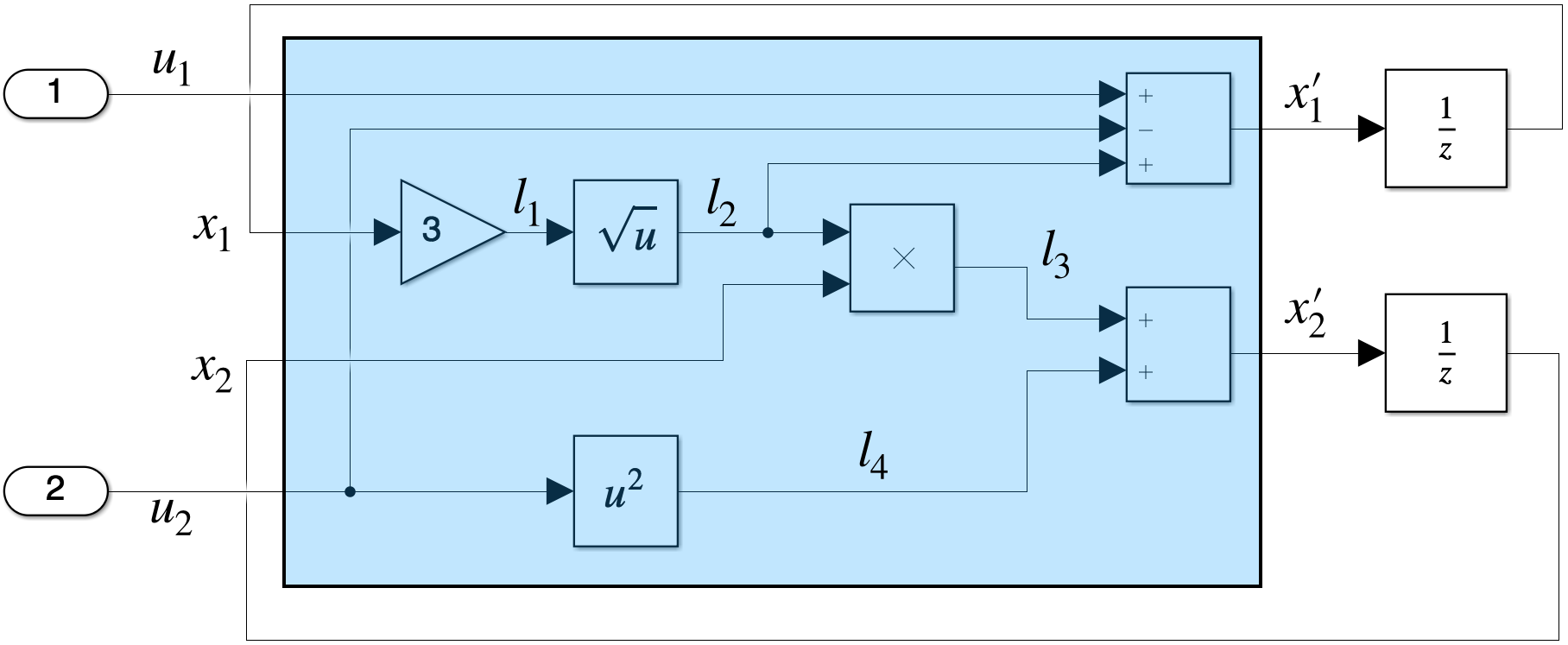
Figure 1: Simulink visualization of Equation 6. The blue box is a composite module consisting of internal modules.

Consider as an example the discrete time control system

$$x^{\prime}:=\mathcal{F}(x,u)$$ (1)

with two continuous current states $x_{1},x_{2}\in\mathbb{R}$, two control inputs $u_{1},u_{2}\in\mathbb{R}$, and two next states $x_{1}^{\prime},x_{2}^{\prime}\in\mathbb{R}$. Let $\mathcal{F}(x,u)$ be concretely given by Equation 6.

$$\left(\begin{array}[]{l}x_{1}^{\prime}\\ x_{2}^{\prime}\end{array}\right):=\left(\begin{array}[]{l}\sqrt{3x_{1}}-u_{2}+u_{1}\\ x_{2}\sqrt{3x_{1}}+u_{2}^{2}\end{array}\right)$$ (6)

The encodings (1) directly maps the variables $u_{1},u_{2},x_{1},x_{2}$ to a next state $x_{1}^{\prime},x_{2}^{\prime}$, but this obfuscates some internal structure that is more clear when the system is viewed as the blue box in Figure 1. Latent variables $l_{1}:=3x_{1}$, $l_{2}:=\sqrt{3x_{1}}$, $l_{3}:=x_{2}\sqrt{3x_{1}}$, and $l_{4}:=u_{2}^{2}$ capture intermediate computations, with $l_{2}$ is also shared across updates for both $x_{1}^{\prime}$ and $x_{2}^{\prime}$.

Modules are analogous to the blue box in Figure 1 and the blocks it contains. They are memoryless and encode the system’s transition relation. Two modules are connected in series if the output of one module feeds into the input of another, such as the gain and square root modules. Two components are connected in parallel if neither output is connected to the other module’s input, such as the summation components. Module composition yields another module. In our framework, unit delay blocks are not considered modules. They only appear to break any algebraic loops and introduce state in the context of controller synthesis, but they are not required for encoding the dynamics $\mathcal{F}(x,u)$.

II Logical System Representations and Notation

The assignment operator “:=” in Equation 6 is problematic because the example can exhibit non-determinism and blocking behaviors, which commonly appear in finite state abstractions as will be shown in Section IV. Under the system dynamics, $x_{1}$ can easily become negative but this induces the system to block because $x_{1}^{\prime}$ and $x_{2}^{\prime}$ are calculated by taking the square root $\sqrt{3x_{1}}$ (we ignore complex numbers). Even if $x_{1}\geq 0$, the square root module may be non-deterministic and output either a positive or negative square root.

Predicates can accommodate both non-determinism and undefined outputs in a unified notation. Predicates are functions that output a Boolean value and can be interpreted as set indicator functions or as constraints to be satisfied. We can replace $x^{\prime}:=\mathcal{F}(x,u)$ with a predicate representation $F(x,u,x^{\prime})$, which only accepts those values of $x,u,x^{\prime}$ where for some $l_{2}$ satisfy each of the following:

$$x_{1}^{\prime} ==l_{2}-u_{2}+u_{1}$$

$$x_{2}^{\prime} ==x_{2}l_{2}+u_{2}^{2}$$

$$l_{2} \in\{|\sqrt{3x_{1}}|,-|\sqrt{3x_{1}}|\}$$

$$x_{1} \geq 0.$$

Section V on module composition will formally show how constraints like those above are generated.

II-A Manipulating Predicates

We briefly introduce predicates and the operations used to manipulate them. A formal introduction is provided in [5].

Let $\top$ denote logical true and $\bot$ denote false. Operators $\neg,\wedge,\vee$ respectively represent negation, conjunction, and disjunction. The implication $a\Rightarrow b$ is a shorthand for the formula $\neg a\vee b$. We use the assignment notation $:=$ for new definitions or declarations. The $==$ operator is a generic equivalence check between two objects of the same type and returns either true or false. Special cases of the equivalence check are set equivalence $\equiv$ and logical equivalence $\Leftrightarrow$.

Variables are denoted by lower case letters and are analogous to wires in Simulink. Each variable $v$ is associated with a domain of values $\mathcal{D}(v)$, which is analogous to the variable’s type. A composite variable is a set of variables and is analogous to a bundle of wires held together by tie wraps. The composite variable $v$ can be constructed by taking a union $v:=v_{1}\cup\ldots\cup v_{M}$ and the domain $\mathcal{D}(v)\equiv\prod_{i=1}^{M}\mathcal{D}(v_{i})$. For example if $v$ is associated with a $M$-dimensional Euclidean space $\mathbb{R}^{M}$, then it is a composite variable that can be broken apart into a collection of atomic variables $v_{1},\ldots,v_{M}$ where $\mathcal{D}(v_{i})\equiv\mathbb{R}$ for all $i:=1,\ldots,M$. All technical results herein do not distinguish between composite and atomic variables.

Predicates are functions that map variable assignments to a Boolean value. Boolean valued expressions like “$x\in\{4,5,12\}$” and “$y==\sin(x)$” are predicates. The variables contained in those expressions are unassigned in the sense that they are not associated with a single value. Once all of a predicate’s variables are assigned, it returns a Boolean value. Predicates without full variable assignments yield newer predicates, e.g. assigning $y=1$ in “$(y==\sin(x))$” yields the predicate “$(1==\sin(x))$”. Assignment of a composite variable $v\equiv v_{1}\cup\ldots\cup v_{M}$ means that every $v_{i}$ is assigned to an element in $\mathcal{D}(v_{i})$. Predicates that stand in for expressions are denoted by capital letters and are often written with the variables that appear within them, e.g. a predicate $P(v,w)$ can stand in for the expression $``v\leq w"$.

Predicate variables are omitted when necessary in order to avoid bloated expressions and notation overhead. For example, $P(v,w)$ can simply be denoted by $P$ when clear from context that it is associated with $v$ and $w$. Moreover, if some variables are composite then the notation can be expanded. That is, if $v\equiv v_{1}\cup\ldots\cup v_{M}$ then $P(v_{1},\ldots,v_{M},w)$ and $P(v,w)$ represent the same predicate.

Predicates can construct sets via set builder notation. A single predicate can instantiate different sets if the domains differ, e.g. $\{x\in\mathcal{D}(x)|P(x)\}$ and $\{(x,y)\in\mathcal{D}(x)\times\mathcal{D}(y)|P(x)\}$ are distinct sets but are associated with the same predicate.

The standard Boolean operations can be applied to a predicate’s Boolean output to construct new predicates. The negated predicate $\neg P(v)$ is true for an assignment to $v$ if and only if $P(v)$ is false. The domain of a predicate obtained via a binary operation is the union of the two variable domains, e.g., conjunction $P(v)\wedge Q(w)$ yields a predicate $(P\wedge Q)(v,w)$. Predicates $P$ and $Q$ are logically equivalent (denoted by $P\Leftrightarrow Q$) if and only if $P\Rightarrow Q$ and $Q\Rightarrow P$ are true for all variable assignments.

The universal quantifier $\forall$ and existential quantifier $\exists$ eliminate predicates variables and are analogous to set projection operations. Given predicate $P(v,w)$, $\exists wP$ and $\forall wP$ are predicates over $v$. An assignment $v\in\mathcal{D}(v)$ satisfies $\exists wP$ if and only if there exists an assignment $w\in\mathcal{D}(w)$ such that $P(v,w)$ evaluates to true. Similarly, an assignment to $v$ satisfies $\forall wP$ if and only if $P(v,w)$ evaluates to true for all assignments $w\in\mathcal{D}(w)$. Applying DeMorgan’s law yields the identities $\neg\exists wP\Leftrightarrow\forall w(\neg P)$ and $\neg\forall wP\Leftrightarrow\exists w(\neg P)$. If the variable to be eliminated does not exist in the predicate, then the same predicate is returned. If the variable $w$ is actually a composite variable $w:=w_{1}\cup\ldots\cup w_{N}$ then $\exists wP$ is simply a shorthand for $\exists w_{1}\ldots\exists w_{N}P$.

III Modules and Their Abstractions

Modules are represented as predicates where each variable is assigned a role as an input or output.

Definition 1 (Modules).

A module is a triple $(i,o,F)$ where $i$ is a set of input variables, $o$ is a set of output variables, and predicate $F(i,o)$ is a joint constraint on variables $i$ and $o$.

For a module that implements a scaling function from input $i$ to output $o$ with fixed gain $\kappa\in\mathbb{R}$, the predicate is given by an equality condition $(o==\kappa i)$. After assigning concrete values to $o$ and $i$, this predicate evaluates to $\top$ or $\bot$.

Control system modules are a special kind of module with state variables $x,x^{\prime}$ satisfying $\mathcal{D}(x)\equiv\mathcal{D}(x^{\prime})$ and a controllable input variable $u$.

Definition 2 (Control System Module).

A time invariant discrete time control system is represented by the module $(x\cup u,x^{\prime},F)$. Variables $x,u,x^{\prime}$ can be composite so the system state and control inputs may be multi-dimensional.

An input’s assignment is blocking if all possible outputs violate the module’s predicate.

Definition 3 (Nonblocking Inputs).

Module $(i,o,F)^{\prime}s$ nonblocking inputs are denoted by the predicate ${NB}_{F}(i):=\exists oF(i,o)$. The blocking inputs are $\neg{NB}_{F}$ or equivalently $\forall o(\neg F)$.

Consider the module $(x,y,\;y==\sqrt{x})$. The nonblocking predicate $\exists y(y==\sqrt{x})$ is equivalent to the input constraint $x\geq 0$ because no assignment to variable $y$ can be equivalent to an undefined value when $x$ is negative. Similarly, for the division module $(x\cup y,z,z==\frac{x}{y})$ the nonblocking predicate ${NB}_{z==\frac{x}{y}}$ reduces down to the expression $y\neq 0$.

III-A Approximate Variable Abstraction

Constructing finite abstractions starts with defining a finite domain that is related to the continuous domain. Consider a generic concrete variable $w$; we denote its associated abstract variable as $\hat{w}$. The quantization relation $Q_{w}(w,\hat{w})$ is a predicate that formalizes the relationship and evaluates to true whenever a pair $w,\hat{w}$ is related. This quantization predicate is called strict if for all assignments to $w$ there exists an assignment to $\hat{w}$ such that $Q_{w}(w,\hat{w})$ evaluates to true. More succinctly, the predicate $\forall w\exists\hat{w}Q_{w}(w,\hat{w})\Leftrightarrow\top$. The relation may be interpreted as a pair of set-valued maps $Q_{w}:\mathcal{D}(w)\rightarrow 2^{\mathcal{D}(\hat{w})}$ and $Q_{w}^{-1}:\mathcal{D}(\hat{w})\rightarrow 2^{\mathcal{D}(w)}$. From this point of view, the relation is strict if and only if $Q_{w}(w)\neq{\varnothing}$ for all assignments to $w$ or, alternatively, if $\cup_{\hat{w}\in\mathcal{D}(\hat{w})}Q_{w}^{-1}(\hat{w})$ is a cover of $\mathcal{D}(w)$. For quantization relations over multiple variables such as $Q_{x\cup y}(x,y,\hat{x},\hat{y})$, we adopt a convention where the relation is decomposed component-wise

$$Q_{x\cup y}(x,y,\hat{x},\hat{y})\Leftrightarrow Q_{x}(x,\hat{x})\wedge Q_{y}(y,\hat{y}).$$ (7)

A common space-discretization pair is a bounded subset of Euclidean space $\mathbb{R}^{N}$ paired with a finite cover of hyperrectangles. For example, the quantization relation $Q_{w}$

$$Q_{w}(w,\hat{w}):=\left(||w-\hat{w}||_{\infty}\leq\frac{\eta}{2}\right)$$ (8)

encodes a cover that consists of infinity-norm balls of diameter $\eta>0$ for a domain $\mathcal{D}(\hat{w})\equiv\{\eta x|x\in\mathbb{Z}^{N}\}$ of discrete points.

Occasionally a concrete variable is already discrete and doesn’t need to be abstracted. In this scenario $w$ and $\hat{w}$ will refer to the same set of variables and we use the identity relation for $Q_{w}(w,\hat{w})$. It is trivially $\top$ because $w,\hat{w}$ can only be assigned to the same value.

III-B Module Approximations

Once each concrete variable is associated with an abstract counterpart, we can establish relationships between abstract and concrete modules.

Definition 4 (Approximate Module Abstraction).

Let $(i,o,M)$ and $(\hat{i},\hat{o},\hat{M})$ be modules and $Q_{i}$ and $Q_{o}$ be strict quantization relations. $\hat{M}$ is an approximation of $M$ with respect to $Q_{i}$ and $Q_{o}$ if and only if substituting predicates $M$ and $\hat{M}$ into

$$(Q_{i}(i,\hat{i})\wedge{NB}_{\hat{M}}(\hat{i}))\Rightarrow{NB}_{M}(i)$$ (9)

and

$$\left(\begin{array}[]{c}Q_{i}(i,\hat{i})\wedge{NB}_{\hat{M}}(\hat{i})\wedge M(i,o)\wedge Q_{o}(o,\hat{o})\\ \Downarrow\\ \hat{M}(\hat{i},\hat{o})\end{array}\right)$$ (13)

yields predicates equivalent to $\top$ for all variable assignments. This relationship is denoted by $\hat{M}\preceq_{i,o}M$.

Definition 4 imposes two main requirements between a concrete and abstract module. First, if $\hat{M}$ does not block for abstract input $\hat{i}$, then any concrete input $i$ associated with $\hat{i}$ via $Q_{i}(i,\hat{i})$ does not block; that is, the abstract component is more aggressive with rejecting invalid inputs. Second, if both systems do not block then the abstract output set is a superset of the concrete function’s output set, modulo a quantization error induced by the gridding of both inputs and outputs. The abstract module is a conservative approximation of the concrete module because the abstraction accepts fewer inputs and exhibits more non-deterministic outputs. Conservatism in this direction ensures that any reasoning done over the abstract models is sound and can be generalized to the concrete model. Controller synthesis tools account for blocking and non-determism in the system [16].

Figure 2: The module $M(x,y)==(|y-\sin(2\pi x)|\leq.15)$ and a valid abstraction. The grid lines depict the quantization relation over a bounded domain $[0,1]\times[-1,1]$. The dark blue area represents the set of valid points for the concrete module $M(x,y)$ and the patterned red boxes represent a valid approximate abstraction $\hat{M}(\hat{x},\hat{y})$. The abstract input boxes that overlap $[.15,.35]$ or $[.65,.85]$ on the $x$ axis are the abstract blocking inputs $\neg{NB}_{\hat{M}}(\hat{x})$.

A feedback refinement relation (FRR) is a specialized instance of Definition 4 for control systems, where the concrete and abstract system have identical control inputs $u$ and $Q_{u}(u,\hat{u})\Leftrightarrow\top$. Definition 5 is identical to the definition introduced in [12] but written as a condition on predicates.

Definition 5 (Feedback Refinement Relation).

Let control system modules $(x\cup u,x^{\prime},{F})$ and $(\hat{x}\cup u,\hat{x}^{\prime},\hat{{F}})$ share a common control variable $u$. A strict relation $Q_{x}$ is a feedback refinement relation from ${F}$ to $\hat{{F}}$ if

$$Q_{x}(x,\hat{x})\wedge{NB}_{\hat{{F}}}(\hat{x},u)\Rightarrow{NB}_{{F}}(x,u)$$ (14)

is true for all assignments to $x,\hat{x},u$ and

$$\left(\begin{array}[]{c}Q_{x}(x,\hat{x})\wedge{NB}_{\hat{{F}}}(\hat{x},u)\wedge Q_{x}(x^{\prime},\hat{x}^{\prime})\\ \wedge{F}(x,u,x^{\prime})\\ \Downarrow\\ \hat{{F}}(\hat{x},u,\hat{x}^{\prime})\end{array}\right)$$ (19)

is true for all assignments to $x,\hat{x},u,x^{\prime},\hat{x}^{\prime}$. Let $\hat{{F}}\preceq_{Q_{x}}{F}$ denote that $Q_{x}$ is a feedback refinement relation from ${F}$ to $\hat{{F}}$.

The most important property of feedback refinement relations is that a controller designed for an abstract system $\hat{{F}}$ can be refined into a controller for the concrete system.

Theorem 1 (Informal Statement of Theorem VI.3 from [12]).

If there exists a controller that enforces a behavior for abstract system $\hat{{F}}$ and $\hat{{F}}\preceq_{Q_{x}}{F}$ then there exists a controller for the concrete system such that the closed loop system satisfies that same behavior, modulo an approximation error with respect to state quantization $Q_{x}$.

The next section describes how finite abstractions are constructed and represented. It resembles existing abstraction methods for continuous state systems and is included for completeness. Readers who are familiar with symbolic control synthesis packages PESSOA[9] or SCOTS[14], and binary decision diagrams may skip directly to Section V, which contains our main technical result on module composition.

IV Constructing Finite Module Abstractions

This section provides background about the data structure used to store predicates over finite domains and an algorithm to construct an abstract predicate via overapproximations of forward reachable sets.

IV-A Storage and Manipulation of Predicates

The efficiency of constructing, storing, and manipulating abstractions depends on their underlying data structure. Hash tables and sparse matrices can be used to store an abstract module’s input-output pairs, but require exponential memory with respect to the module input dimensionality.

The storage and manipulation problems are mitigated by representing the system and interconnection abstractions with ordered binary decision diagrams (BDDs) [1], a data structure that compactly represents predicates by detecting symmetries and redundant structure. BDDs are an implicit representation and often exhibit a smaller memory footprint compared to explicit representations that store every transition in memory. The CUDD toolbox [15] provides functionality for common operations such as taking conjunctions, disjunctions, negations, variable renaming, equality checking, and existential/universal quantification over a set of variables. These operations are performed directly on BDDs and have been empirically observed to be more memory and time efficient than analogous operations implemented for lookup tables [2].

IV-B Abstraction via Module Input Space Traversal

If quantization relations $Q_{i}^{-1}$ and $Q_{o}$ are viewed as set-valued maps $Q_{i}^{-1}:\hat{i}\rightarrow 2^{i}$ and $Q_{o}:o\rightarrow 2^{\hat{o}}$, then the tightest overapproximation of $F:i\rightarrow o$ can be obtained by the composition of functions $Q_{o}(F(Q_{i}^{-1}(\hat{i})))$. This composition can be viewed as a quantized version of a one step reachability problem where the image of the set of points contained in the partition $Q_{i}^{-1}(\hat{i})$ under the map $F$ is computed.

Exact characterizations of reachable sets for arbitrary systems do not exist, but there are several practical methods to compute overapproximations $OA:\hat{i}\rightarrow 2^{\hat{o}}$ that satisfy the set containment condition $Q_{o}(F(Q_{i}^{-1}(\hat{i})))\subseteq OA(\hat{i})$. A few overapproximation procedures are available when a dense subset of Euclidean space is partitioned into hyper-rectangular regions. Consider a generic module $F:\mathbb{R}^{m}\rightarrow\mathbb{R}^{n}$ and a hyper-rectangle $[a,b]$ defined by the two corners $a,b\in\mathbb{R}^{m}$ where $a_{i}\leq b_{i}$ for all $i=1,\ldots,m$. Component-wise Lipschitz bounds and monotonicity are two common methods to overapproximate $F([a,b])$.

Example 1 (Component-wise Lipschitz Bounds).

Let $c:=\frac{1}{2}(a+b)$ and $r:=\frac{1}{2}(b-a)$. Let $L$ be a matrix with non-negative entries satisfying $|F(y)-F(x)|\leq L|y-x|$ for all $x,y$ where the absolute values and inequality are component-wise. The hyper-rectangle $[F(c)-Lr,F(c)+Lr]$ is a superset of $F([a,b])$.

Example 2 (Monotone Functions).

If $F$ is a monotone function, then $[F(a),F(b)]$ is a superset of $F([a,b])$.

Algorithm 1 is a procedure that only uses evaluations of $OA$ to construct a finite abstraction.

Algorithm 1 Module Abstraction Pseudo Code

1:function AbstractModule(Overapprox. $OA:\hat{i}\to 2^{\hat{o}}$)

2:     $\hat{F}:=\bot$ $\triangleright$ No transitions initially

3:     for all $[a]\in Q_{i}^{-1}(\mathcal{D}(\hat{i}))$ do $\triangleright$ Input Grid Traversal

4:         $T^{\prime}:=\bot$

5:         if $OA([a]))\not\subseteq Q_{o}^{-1}(\mathcal{D}(\hat{o}))$ then

6:              continue $\triangleright$ Imposes blocking input          

7:         for all $[b]\in Q_{o}(OA([a]))$ do

8:              $T^{\prime}:=T^{\prime}\vee(\hat{o}==[b])$ $\triangleright$ Construct output set          

9:         $\hat{F}:=\hat{F}\vee\left((\hat{i}==[a])\wedge T^{\prime}\right)$ $\triangleright$ Adds transitions

10:         return $\hat{F}$      

Note that $[a]$ and $[b]$ represent specific values of the abstract input and output sets; this value changes with each iteration of the loops in lines 3 and 7. Line 5 checks for out of bounds errors, which are common when the concrete domain is Euclidean space and the abstract domain corresponds to a finite cover with bounded subsets. For instance, an unstable system may exit the bounded region covered by the abstract outputs for inputs that do not stabilize the system. The continue command on the next line causes the abstract system to block for that input by preventing any transition from being added. Blocking inputs are accounted for within the synthesis procedure [16]. If the system does not block, then the loop on line 7 constructs the output set and line 9 adds the input-output pairs to the predicate.

Line 3 of Algorithm 1 is a nested loop with depth equal to the dimension of the input grid and is the source of the exponential runtime. Breaking apart a larger system into smaller modules and abstracting those limits the dimension of the largest module’s input grid. Existing tools PESSOA [9] and SCOTS[14]construct symbolic representations by applying Algorithm 1 directly on a monolithic control system.

V Module Composition

We model connections between modules implicitly via shared variables, which represent the wires between modules and the module ports they connect. Module behaviors are coupled because variables can only assume one value. Connections between modules can be made simply by renaming variables. We adopt a module composition operation from [17] that can be applied to both concrete and abstract modules.

Definition 6 (Module Composition).

Let $(i_{1},o_{1},M_{1})$ and $(i_{2},o_{2},M_{2})$ be modules with disjoint output variables $o_{1}\cap o_{2}={\varnothing}$. Without loss of generality, let $io_{12}:=o_{1}\cap i_{2}$ and

$$i_{1}\cap o_{2}\equiv{\varnothing}$$ (20)

signifying that outputs of module $M_{2}$’s may not be fed back into inputs of $M_{1}$. Define new composite variables

$$i_{12} :=(i_{1}\cup i_{2})\setminus io_{12}$$ (21)

$$o_{12} :=o_{1}\cup o_{2}$$ (22)

and the composed module $(i_{12},o_{12},M_{12})$ with predicate

$$M_{12} :=M_{1}(i_{1},o_{1})\wedge M_{2}(i_{2},o_{2})$$ (23)

$$\qquad\qquad\wedge\forall o_{12}(M_{1}(i_{1},o_{1})\Rightarrow{NB}_{M_{2}}(i_{2}))$$

The module subscripts may be swapped if instead the outputs of $M_{2}$ are fed into $M_{1}$.

We say that $M_{12}$ is a parallel composition of $M_{1}$ and $M_{2}$ if $io_{12}\equiv{\varnothing}$ holds in addition to Equation 20. Equation 23 under parallel composition reduces down to $M_{1}\wedge M_{2}$ (Lemma 6.4 in [17]) and the composition operation is both commutative and associative. If $io_{12}\not\equiv{\varnothing}$, the modules are composed in series and the composition operation is only associative.

The last term in Equation 23 is a predicate over the expanded input set $i_{12}$ and deals with blocking behaviors under series composition. It disallows inputs whenever there exists an output of $M_{1}$ that causes $M_{2}$ to block. The new module’s nonblocking inputs ${NB}_{M_{12}}$ are:

$${NB}_{M_{12}}:=\exists o_{12}(M_{1}\wedge M_{2})\wedge\forall o_{12}(M_{1}\Rightarrow{NB}_{M_{2}}).$$ (24)

Figure 3 explains the role of the right-most term for a series composition of generic modules, but we also include a concrete example.

Example 3.

Consider a module $(x,y,M_{1})$ with predicate $M_{1}(x,y):=(|y-x|\leq 2)$, which feeds into a module $(y,z,M_{2})$ with predicate $M_{2}(y,z):=(z==\sqrt{y})$. $M_{2}$’s nonblocking inputs ${NB}_{M_{2}}(y)$ are $(y\geq 0)$. Substituting into the term $\exists o_{12}(M_{1}\wedge M_{2})$ from Equation 24 yields

$$\exists y\exists z(|y-x|\leq 2\wedge z==\sqrt{y})\Leftrightarrow(x\geq-2)$$

because for any $x\geq-2$ the assignments $y:=x+2$ and $z:=\sqrt{x+2}$ satisfy the expression. However the serial composition is not robust to an adversarial assignment to $y$, e.g. $x=-1,y=-1$. Substituting into the term $\forall o_{12}(M_{1}\Rightarrow{NB}_{M_{2}})$ from (24) yields a tighter constraint on inputs.

$$\forall y\forall z(|y-x|\leq 2\Rightarrow y\geq 0)$$

$$\quad\Leftrightarrow\forall y(|y-x|>2\vee y\geq 0)$$

$$\qquad\Leftrightarrow(x\geq 2).$$

Any input $x<2$ is disallowed because there exists a strictly negative $y$ that satisfies $|y-x|\leq 2$.

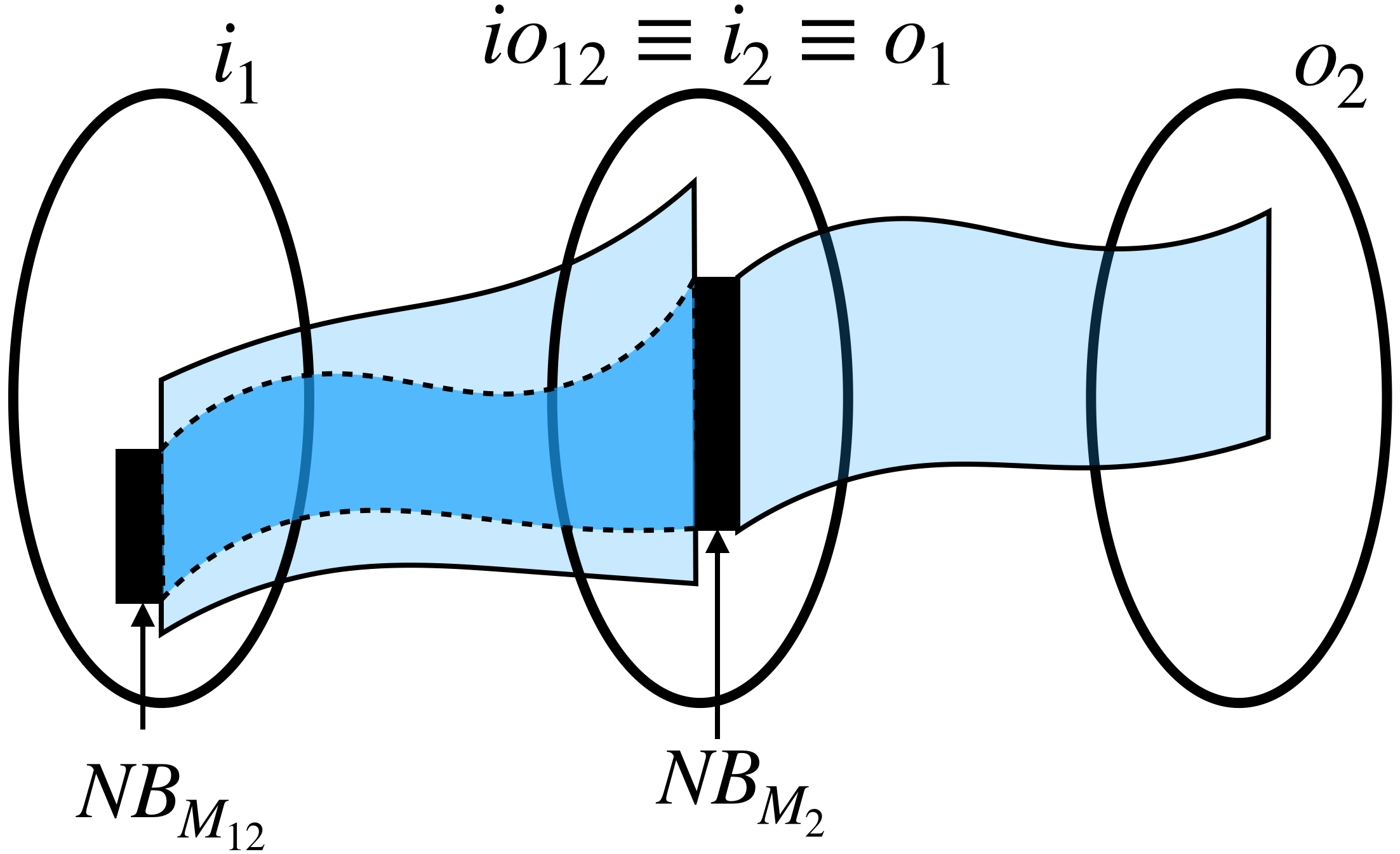
Figure 3: Visualization of the propagation of nonblocking inputs under series composition from Definition 6. Module $M_{2}$’s nonblocking set ${NB}_{M_{2}}$ is a strict subset of the possible outputs of module $M_{1}$. Some nonblocking inputs to $M_{1}$ may lead $M_{2}$ to block instead. The additional constraint $\forall io_{12}(M_{1}\Rightarrow{NB}_{M_{2}})$ causes ${NB}_{M_{12}}$ to prune inputs to $M_{1}$ that could induce $M_{2}$ to block under an adversarial choice of $o_{1}$, even though those inputs would not cause $M_{1}$ to block.

Algorithm 2 Compose a Collection of Modules

1:function Comp(Modules $M_{1},\ldots,M_{N}$)

2:No algebraic loop in $G$

3:     Construct dependency graph $G$

4:     $s_{1},\ldots,s_{N}$ := TopologicalSort($G$) $\triangleright$ System Indices

5:     ${F}:=({\varnothing},{\varnothing},\top)$ $\triangleright$ Initialize Empty Module

6:     for ($j:=1;j\leq N;j:=j+1$) do

7:         ${F}:=\textsf{Comp}(M_{s_{j}},{F})$ $\triangleright$ From Definition 6      

8:     return ${F}$

Algorithm 2 is used to compose a collection of modules through systematic application of the binary module composition operator from Definition 6. It first constructs a directed dependency graph where all vertices are modules and an edge exists from $M_{1}$ to $M_{2}$ if $o_{1}\cap i_{2}\neq{\varnothing}$ (i.e., outputs of $M_{1}$ feed into $M_{2}$). We assume that the constructed graph is directed and acyclic; this requirement ensures that there are no algebraic loops. The graph can be topologically sorted into a sequence of indices $s_{1},\ldots,s_{N}\in\{1,\ldots,N\}$ where a directed edge from $M_{s_{i}}$ to $M_{s_{j}}$ implies that $s_{j}<s_{i}$. This would cause “downstream” module $M_{2}$ to come before “upstream” $M_{1}$. The topological sort is necessary because composing modules in any arbitrary order may violate the requirement in Equation 20 by introducing circular dependencies and feedback composition. Although the topological sort does not necessarily yield a unique linear module ordering, associativity and commutativity of the composition operation ensures that Algorithm 2’s output is unique.

Composing a large collection of variables cause the number of outputs to grow. The output hiding operator can be used to ignore superfluous module outputs.

Definition 7 (Output Hiding).

Hiding $(i,o\cup w,M)$’s output $w$ yields the module $(i,o,\exists wM)$.

Existentially quantifying out the hidden variable ensures that the input-output behavior over the unhidden variables is still consistent with the behaviors with the hidden variable.

Control modules $(x\cup u,x^{\prime},F)$ only have next state variables $x^{\prime}$ as outputs. A control system can be obtained by composing a set of components using Algorithm 2 and hiding all latent variables that become outputs as a result of series composition.

V-A Main Result: Module Composition and Output Hiding Preserve Approximate Abstraction Relations

The following theorems show that the composition and output hiding operators preserve the relation between abstract and concrete modules. Proofs are provided in the appendix.

Theorem 2.

Let $\hat{M}_{1}\preceq_{i_{1},o_{1}}M_{1}$ and $\hat{M}_{2}\preceq_{i_{2},o_{2}}M_{2}$ and modules $M_{12}$ and $\hat{M}_{12}$ be the resulting composed modules from Definition 6. Then $\hat{M}_{12}\preceq_{i_{12},o_{12}}M_{12}$.

Theorem 3.

If $\hat{M}\preceq_{i,o_{1}\cup o_{2}}M$ for modules $(i,o_{1}\cup o_{2},M)$ and $(\hat{i},\hat{o}_{1}\cup\hat{o}_{2},\hat{M})$, then $\exists\hat{o}_{2}\hat{M}\preceq_{i,o_{1}}\exists o_{2}M$.

Because control systems are modules and feedback refinement relations are a special case of Definition 4, it readily follows that control systems can be constructed from module composition and variable hiding.

While Theorems 2 and 3 show that abstractions are preserved under composition, unnecessarily decomposing a system may destroy structural properties and introduce additional non-determinism. For example, let a concrete module $(x,y,y==3x)$ and its inverse $(y,z,z==\frac{y}{3})$ be composed in series and the $y$ output hidden, yielding the identity module $(x,z,z==x)$. Discretizing the variable $y$ first breaks the identity relationship between the two concrete modules, so composing abstract modules induces more non-determinism than abstracting the identity module directly.

VI Related Work

This paper generalizes the core insights from [4] and [7]. High dimensional system abstractions are constructed via parallel system composition [4], but the computational gains are most dramatic when the dynamics inherently exhibited a locality property where states are independent of one another. A limited form of series composition is introduced in [7] to further decompose the system, but it is unable to handle blocking inputs because it does not include the right-most term in Equation 23. Instead of feedback refinement relations, it was based on alternating simulation relations and required that each control input be associated with a unique component.

This paper differs from the existing literature on large-scale controller synthesis, which generally aims to solve a decentralized control problem where multiple agents each have control over a local control input and need to jointly satisfy some property. Guaranteeing satisfaction is difficult due to coupled system dynamics, concurrent decision making, and controllers only having access to local information. Many existing results certifying correctness of a decentralized controller assume a decomposed specification and rely on a certificate that the actions of an individual controller do not interfere with another controller’s ability to satisfy its specification. This certificate ensures soundness of the decomposed synthesis procedure and may come in the form of a stability certificate [13, 19, 8], assume-guarantee constraints [10, 6]. Finding a suitable system decomposition often case specific, restricting the portability of the decomposed controller synthesis results.

VII Example

We consider a set of $N$ single-input scalar systems where $\mathcal{D}(x_{i}):=[0,32]$, $\mathcal{D}(u_{i}):=\{-2,-1,1,2\}$ for each $i=1,\ldots,N$. The dynamics for the $i$-th update are given by

$$x_{i}^{\prime}==\text{GLOG}_{[0,32]}(x_{i}+u_{i}+k(x_{i}-l_{1}))$$ (25)

where $k=0.2$ and $\text{GLOG}_{[0,31]}(\cdot)$ is a generalized logistic function with output values within the range $[0,32]$

$$\text{GLOG}_{[0,32]}(x)==\frac{32}{1+e^{-.2(x-\frac{b+a}{2})}}.$$ (26)

The latent variable $l_{1}$ encodes the average state

$$l_{1}==\frac{1}{N}\sum_{i=1}^{N}x_{i}.$$ (27)

Using Algorithm 1 to directly construct the module (27) requires iterating over a joint state space $\prod_{i=1}^{N}\mathcal{D}(x_{i})$. When $N=6$ this is computationally prohibitve, so we introduce two latent variables $l_{2},l_{3}$ representing intermediate averages

$$l_{2}==\frac{1}{3}\left(x_{1}+x_{2}+x_{3}\right)\quad\text{ and }\quad l_{3}==\frac{1}{3}\left(x_{4}+x_{5}+x_{6}\right).$$

The above equations and (28) below are equivalent to (27).

$$l_{1}==\frac{1}{2}\left(l_{2}+l_{3}\right).$$ (28)

By construction, all latent variables lie within the space $[0,32]\equiv\mathcal{D}(l_{1})\equiv\mathcal{D}(l_{2})\equiv\mathcal{D}(l_{3})$. We discretize each continuous space $x_{i}$ into 32 bins and the input space is already discrete. Constructing abstractions for all nine modules takes a total of $1.53$ seconds. There are six modules $(x\cup u_{i},x_{i}^{\prime},F_{i})$ that constrain each output $x_{i}^{\prime}$. These modules are constructed over a total of $20.35$ seconds via series composition and hiding the abstract latent variables $\hat{l}_{1},\hat{l}_{2},\hat{l}_{3}$. These six modules are then composed in parallel over $343.02s$ to obtain the final monolithic system which has $8.80\times 10^{14}$ transitions. Abstracting the control system monolithically requires a traversal over a grid of $4.4\times 10^{12}\approx(32\times 4)^{6}$ state-control pairs and does not terminate after running 8 hours. All benchmarks are run on a standard laptop with $8$GB of RAM and a 2.4 GHz quad-core processor with a modified version of SCOTS. Other benchmarks with fewer discrete states and transitions have required tens of hours [11] and hundreds of gigabytes of RAM [18] to compute and store abstractions. Although these benchmarks had different hardware and software implementations, they highlight how a monolithic approach to abstraction quickly grows intractable.

Appendix A Proofs of Theorems 2 and 3

Proof of Theorem 2.

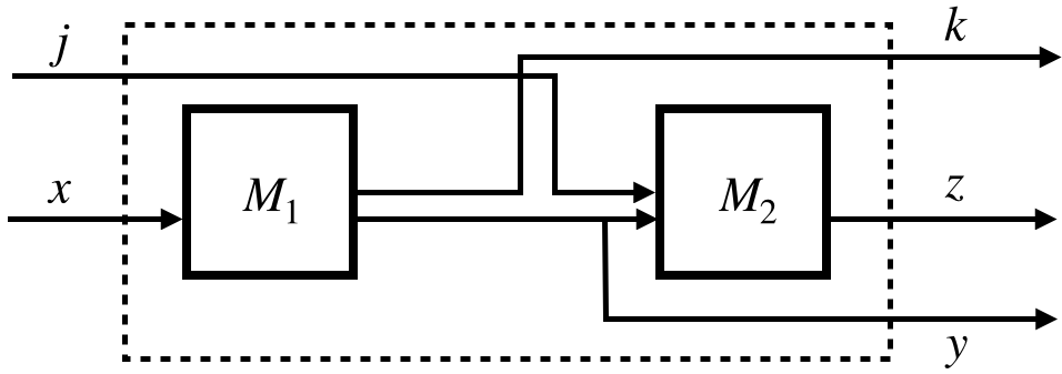
Figure 4: Generic composition of concrete modules used in Theorem 2’s proof.

Consider two modules $(x,k\cup y,M_{1})$, $(j\cup y,z,M_{2})$. Figure 4 depicts a general interconnection where $io_{12}\equiv y$ is a subset of the outputs of $M_{1}$ and inputs of $M_{2}$. It follows that $M_{12}=(x\cup j,y\cup k\cup z,M_{12})$ where the input-output behavior is constrained by the predicate

$$M_{12}:=\; M_{1}\wedge M_{2}\wedge\forall y\forall k\forall z(M_{1}\Rightarrow{NB}_{M_{2}})$$ (29)

$$:=\; M_{1}\wedge M_{2}\wedge\forall y(\forall kM_{1}\Rightarrow{NB}_{M_{2}}).$$ (30)

Predicate ${NB}_{M_{12}}(x,j)$ encodes the set of nonblocking inputs:

$${NB}_{M_{12}} :=\exists y\exists k\exists z(M_{1}\wedge M_{2}\wedge\forall y(\forall kM_{1}\Rightarrow{NB}_{M_{2}}))$$

$$:=\exists y(\exists kM_{1}\wedge{NB}_{M_{2}})\wedge\forall y(\forall kM_{1}\Rightarrow{NB}_{M_{2}}).$$

From Theorem 2’s assumptions it is known that $\hat{M}_{1}\preceq_{x,k\cup y}M_{1}$ and $\hat{M}_{2}\preceq_{j\cup y,z}M_{2}$. These conditions written explicitly are the overapproximation condition on $M_{1}$

$$\begin{array}[]{c}Q_{x\cup y\cup k}(x,\hat{x},y,\hat{y},k,\hat{k})\wedge{NB}_{\hat{M}_{1}}(\hat{x})\wedge M_{1}(x,k,y)\\ \Downarrow\\ \hat{M}_{1}(\hat{x},\hat{k},\hat{y})\end{array}$$ (34)

the overapproximation condition on $M_{2}$

$$\begin{array}[]{c}Q_{j\cup y\cup z}(j,\hat{j},y,\hat{y},z,\hat{z})\wedge{NB}_{\hat{M}_{2}}(\hat{j},\hat{y})\wedge M_{2}(j,y,z)\\ \Downarrow\\ \hat{M}_{2}(\hat{j},\hat{y},\hat{z})\end{array}$$ (38)

and the nonblocking conditions

$$Q_{x}(x,\hat{x})\wedge{NB}_{\hat{M}_{1}}(\hat{x}) \Rightarrow{NB}_{M_{1}}(x)$$ (39)

$$Q_{j}(j,\hat{j})\wedge Q_{y}(y,\hat{y})\wedge{NB}_{\hat{M}_{2}}(\hat{j},\hat{y}) \Rightarrow{NB}_{M_{2}}(j,y).$$ (40)

We first prove the overapproximation condition from Definition 4 for $M_{12}$.

$$\begin{array}[]{c}Q_{x\cup j\cup y\cup k\cup z}(x,\hat{x},j,\hat{j},y,\hat{y},k,\hat{k},z,\hat{z})\wedge M_{12}(x,j,y,k,z)\\ \wedge{NB}_{\hat{M}_{12}}(\hat{x},\hat{j})\\ \Downarrow\\ \hat{M}_{1}(\hat{x},\hat{k},\hat{y})\wedge\hat{M}_{2}(\hat{j},\hat{y},\hat{z})\wedge\forall\hat{y}(\forall\hat{k}\hat{M}_{1}\Rightarrow{NB}_{\hat{M}_{2}})\end{array}$$ (45)

Suppose that all concrete and abstract variables are assigned such that the upper half of (45) is true. The term $\forall\hat{y}(\forall\hat{k}\hat{M}_{1}\Rightarrow{NB}_{\hat{M}_{2}})$ follows directly from ${NB}_{\hat{M}_{12}}(\hat{x},\hat{j})$. Satisfaction of ${NB}_{\hat{M}_{12}}(\hat{x},\hat{j})$ implies satisfaction of ${NB}_{\hat{M}_{1}}(\hat{x})$, which via Equation 34 implies satisfiaction of $\hat{M}_{1}(\hat{x},\hat{k},\hat{y})$. Satifaction of ${NB}_{\hat{M}_{2}}(\hat{j},\hat{y})$ can now be established because $\hat{M}_{1}(\hat{x},\hat{k},\hat{y})$ is true and $\hat{x}$ and $\hat{j}$ are assigned to value where $\forall\hat{y}(\forall\hat{k}\hat{M}_{1}\Rightarrow{NB}_{\hat{M}_{2}})$ and the specific value of $\hat{y}$ is irrelevant. The upper half of (38) is now satisfied, implying that $\hat{M}_{2}(\hat{j},\hat{y},\hat{z})$ is true. We have proven the bottom half of (45).

We next prove the nonblocking condition for $M_{12}$

$$\begin{array}[]{c}Q_{x}(x,\hat{x})\wedge Q_{j}(j,\hat{j})\\ \wedge\exists\hat{y}(\exists\hat{k}\hat{M}_{1}\wedge{NB}_{\hat{M}_{2}})\wedge\forall\hat{y}(\forall\hat{k}\hat{M}_{1}\Rightarrow{NB}_{\hat{M}_{2}})\\ \Downarrow\\ \exists y(\exists kM_{1}\wedge{NB}_{M_{2}})\wedge\forall y(\forall kM_{1}\Rightarrow{NB}_{M_{2}})\end{array}$$ (50)

Suppose that (50) does not hold, which means that the following formula is satisfiable.

$$Q_{x}(x,\hat{x})\wedge Q_{j}(j,\hat{j})$$ (51)

$$\wedge\exists\hat{y}(\exists\hat{k}\hat{M}_{1}\wedge{NB}_{\hat{M}_{2}})\wedge\forall\hat{y}(\forall\hat{k}\hat{M}_{1}\Rightarrow{NB}_{\hat{M}_{2}})$$

$$\wedge\big{(}\forall y(\forall k\neg M_{1}\vee\neg{NB}_{M_{2}})\vee\neg\forall y(\forall kM_{1}\Rightarrow{NB}_{M_{2}})\big{)}$$

We show that any satisfying assignment leads to a contradiction. Let $x,\hat{x},j,\hat{j}$ be an assignment such that (51) is true. The premises of (39) are implied by the clauses $Q_{x}(x,\hat{x})$ and $\exists\hat{y}(\exists\hat{k}\hat{M}_{1}\wedge{NB}_{\hat{M}_{2}})$ and thus there exist assignments $x,y,k$ such that $M_{1}(x,k,y)$ is satisfied.

We prove that $\forall y(\forall kM_{1}\Rightarrow{NB}_{M_{2}})$ must be false. If it is true, then $\forall y(\forall k\neg M_{1}\vee\neg{NB}_{M_{2}})$ must be hold for (51) to be satisfied. For the assignments $x,j,k,y$ such that $M_{1}(x,k,y)$ is true, these two statements cannot both hold since the former implies ${NB}_{M_{2}}$ while the latter implies $\neg{NB}_{M_{2}}$.

Our problem is now simplified to proving that

$$Q_{x}(x,\hat{x})\wedge Q_{j}(j,\hat{j})$$ (52)

$$\wedge\exists\hat{y}(\exists\hat{k}\hat{M}_{1}\wedge{NB}_{\hat{M}_{2}})\wedge\forall\hat{y}(\forall\hat{k}\hat{M}_{1}\Rightarrow{NB}_{\hat{M}_{2}})$$

$$\wedge(\neg\forall y(\forall kM_{1}\Rightarrow{NB}_{M_{2}}))$$

is a contradiction. The prior assignments to $x,\hat{x},j,\hat{j}$ satisfy Equation 52 whose last clause implies that there must exist assignments $y,k$ such that $M_{1}\wedge\neg{NB}_{M_{2}}$. Invoking strictness of $Q_{k}$ and $Q_{y}$, allows us to assign $\hat{k},\hat{y}$ such that $Q_{k}(k,\hat{k})$ and $Q_{y}(y,\hat{y})$ are true and use Equation 34 such that $\hat{M}_{1}(\hat{x},\hat{k},\hat{y})$ is satisfied. Given all the assigned variables, we can now conclude that ${NB}_{\hat{M}_{2}}$ holds because of $\forall\hat{y}(\forall\hat{k}\hat{M}_{1}\Rightarrow{NB}_{\hat{M}_{2}})$. However the assignment should also satisfy $\neg{NB}_{M_{2}}$, which implies through the contrapositive of Equation 40 that $\neg Q_{j}(j,\hat{j})\vee\neg Q_{y}(y,\hat{y})\vee\neg{NB}_{\hat{M}_{2}}$. Variables $j,\hat{j},y,\hat{y}$ were already assigned so $Q_{j}(j,\hat{j})$ and $Q_{y}(y,\hat{y})$ are true, so ${NB}_{\hat{M}_{2}}$ must be false. Contradiction.

∎

Proof of Theorem 3.

Substitute Definition 7 of a hidden variable module into the conditions from Definition 4. The nonblocking condition (9) only pertains to inputs and so remains unchanged after substitution. Substitution into the overapproximation condition (13) yields the constraint.

$$\left(\begin{array}[]{c}Q_{i}(i,\hat{i})\wedge{NB}_{\hat{M}}(\hat{i})\wedge\exists o_{2}.M(i,o_{1},o_{2})\wedge Q_{o_{1}}(o_{1},\hat{o}_{1})\\ \Downarrow\\ \exists\hat{o}_{2}.\hat{M}(\hat{i},\hat{o}_{1},\hat{o}_{2})\end{array}\right)$$ (56)

Consider assignments to variables $i,\hat{i},o_{1},\hat{o}_{1}$ such that the upper half of (56) holds. Satisfaction of $\exists o_{2}.M(i,o_{1},o_{2})$ implies that there must exist an assignment to $o_{2}$ such that $M(i,o_{1},o_{2})$ holds. Strictness of $Q_{o_{2}}$ implies existence of an assignment to $\hat{o}_{2}$ such that $Q_{o_{2}}(o_{2},\hat{o}_{2})$ holds. Consider any such assignment. By hypothesis $\hat{M}\preceq_{i,o_{1}\cup o_{2}}M$, and all the variables have been assigned to imply satisfaction of $\hat{M}(\hat{i},\hat{o}_{1},\hat{o}_{2})$. It follows that $\exists\hat{o}_{2}.\hat{M}(\hat{i},\hat{o}_{1},\hat{o}_{2})$ is satisfied. ∎

References

- [1] R. E. Bryant. Graph-Based Algorithms for Boolean Function Manipulation. IEEE Transactions on Computers, 35(8):677–691, 1986.
- [2] O. L. Bulancea, P. Nilsson, and N. Ozay. Nonuniform abstractions, refinement and controller synthesis with novel BDD encodings. CoRR, abs/1804.04280, 2018.
- [3] S. Coogan and M. Arcak. Efficient finite abstraction of mixed monotone systems. In Proceedings of 18th International Conference on Hybrid Systems: Computation and Control, pages 58–67, April 2015.
- [4] F. Gruber, E. Kim, and M. Arcak. Sparsity-aware finite abstraction. In 2017 IEEE 56th Conference on Decision and Control (CDC), Dec 2017.
- [5] M. Huth and M. Ryan. Logic in Computer Science: Modelling and reasoning about systems. Cambridge university press, 2004.
- [6] E. S. Kim, M. Arcak, and S. A. Seshia. Compositional controller synthesis for vehicular traffic networks. In Decision and Control (CDC), 2015 IEEE 54th Annual Conference on, pages 6165–6171. IEEE, 2015.
- [7] E. S. Kim, M. Arcak, and M. Zamani. Constructing control system abstractions from modular components. In Proceedings of the 21st International Conference on Hybrid Systems: Computation and Control (Part of CPS Week), HSCC ’18, pages 137–146. ACM, 2018.
- [8] K. Mallik, A.-K. Schmuck, S. Soudjani, and R. Majumdar. Compositional abstraction-based controller synthesis for continuous-time systems. arXiv preprint arXiv:1612.08515, 2016.
- [9] M. Mazo, A. Davitian, and P. Tabuada. PESSOA: A Tool for Embedded Controller Synthesis. In 22nd International Conference on Computer Aided Verification, pages 566–569. Springer, 2010.
- [10] P. J. Meyer, A. Girard, and E. Witrant. Compositional abstraction and safety synthesis using overlapping symbolic models. IEEE Transactions on Automatic Control, 2017, accepted.
- [11] P. Nilsson, O. Hussien, A. Balkan, Y. Chen, A. D. Ames, J. W. Grizzle, N. Ozay, H. Peng, and P. Tabuada. Correct-by-construction adaptive cruise control: Two approaches. IEEE Transactions on Control Systems Technology, 24(4):1294–1307, 2016.
- [12] G. Reißig, A. Weber, and M. Rungger. Feedback refinement relations for the synthesis of symbolic controllers. IEEE Transactions on Automatic Control, 62(4):1781–1796, April 2017.
- [13] M. Rungger and M. Zamani. Compositional construction of approximate abstractions of interconnected control systems. IEEE Transactions on Control of Network Systems, PP(99):1–1, 2016.
- [14] M. Rungger and M. Zamani. SCOTS: A Tool for the Synthesis of Symbolic Controllers. In 19th International Conference on Hybrid Systems: Computation and Control, pages 99–104. ACM, 2016.
- [15] F. Somenzi. CUDD: CU Decision Diagram Package. http://vlsi.colorado.edu/~fabio/CUDD/, 2015. Version 3.0.0.
- [16] P. Tabuada. Verification and Control of Hybrid Systems. New York, NY,USA: Springer, 2009.
- [17] S. Tripakis, B. Lickly, T. A. Henzinger, and E. A. Lee. A theory of synchronous relational interfaces. ACM Transactions on Programming Languages and Systems (TOPLAS), 33(4):14, 2011.
- [18] A. Weber, M. Rungger, and G. Reissig. Optimized state space grids for abstractions. IEEE Transactions on Automatic Control, 62(11):5816–5821, 2017.
- [19] M. Zamani and M. Arcak. Compositional abstraction for networks of control systems: A dissipativity approach. IEEE Transactions on Control of Network Systems, 2017.
- [20] M. Zamani, G. Pola, M. M. Jr., and P. Tabuada. Symbolic models for nonlinear control systems without stability assumptions. IEEE Transaction on Automatic Control, 57(7):1804–1809, July 2012.