Learning to guide task and motion planning using score-space representation

Abstract

In this paper, we propose a learning algorithm that speeds up the search in task and motion planning problems. Our algorithm proposes solutions to three different challenges that arise in learning to improve planning efficiency: what to predict, how to represent a planning problem instance, and how to transfer knowledge from one problem instance to another. We propose a method that predicts constraints on the search space based on a generic representation of a planning problem instance, called score-space, where we represent a problem instance in terms of the performance of a set of solutions attempted so far. Using this representation, we transfer knowledge, in the form of constraints, from previous problems based on the similarity in score space. We design a sequential algorithm that efficiently predicts these constraints, and evaluate it in three different challenging task and motion planning problems. Results indicate that our approach performs orders of magnitudes faster than an unguided planner.

Abstract

In this paper, we propose a learning algorithm that speeds up the search in task and motion planning problems. Our algorithm proposes solutions to three different challenges that arise in learning to improve planning efficiency: what to predict, how to represent a planning problem instance, and how to transfer knowledge from one problem instance to another. We propose a method that predicts constraints on the search space based on a generic representation of a planning problem instance, called score-space, where we represent a problem instance in terms of the performance of a set of solutions attempted so far. Using this representation, we transfer knowledge, in the form of constraints, from previous problems based on the similarity in score space. We design a sequential algorithm that efficiently predicts these constraints, and evaluate it in three different challenging task and motion planning problems. Results indicate that our approach performs orders of magnitudes faster than an unguided planner.

1 1. Introduction

Task and motion planning (TAMP) problems are sequential decision making problems in which a robot is required to search for a sequence of decisions that account for both discrete and continuous aspects of the world to achieve a high-level goal. These decisions are intricately related to one another, and they must abide by collision-constraints and transition dynamics.

A variety of planners have been developed for TAMP problems (Gravot et al.,, 2005; Kaelbling and Lozano-Pérez,, 2013; Lozano-Pérez and Kaelbling,, 2014; Srivastava et al.,, 2014; Toussaint,, 2015; Dantam et al.,, 2017). However, their worst-case computation time generally scales exponentially with problem size, and each new problem instance must be solved from scratch, making them inefficient for real-world tasks. In contrast, humans are able to short-cut their planning process by learning to adapt previous planning experience to reduce the search space intelligently for new problem instances. This observation motivates the design of an algorithm that learns from experience to make predictions that guide the search of a planner. We face three important questions in designing the learning algorithm: (1) what to predict, (2) how to represent a problem instance, and (3) how to transfer knowledge from past experience to the current problem instance.

Figure 1: The task is to pick up the blue object by planning a collision-free path from an initial configuration to a pre-grasp configuration. When the obstacle (pink cup) moves even by 0.02m, this requires a qualitatively different collision-free path.

The first challenge is what to predict. Previous approaches to using learning to speed up planning have tried predicting a complete solution, or a subgoal that fully specifies the robot configuration and world state, including object poses. However, because of the intricate relationship between object poses and the robot’s free-space, a small change in the environment may completely alter the space of feasible solutions. This lack of regularity in the relationship between a problem instance and its solution makes it difficult to predict a complete solution or a subgoal based on experience. This difficulty is illustrated in Figure 1 in a pick domain.

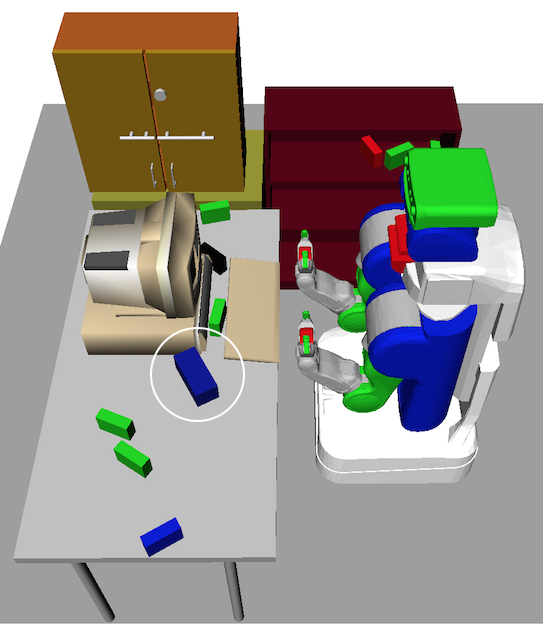
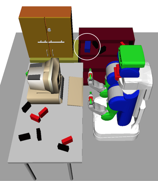
Figure 2: Two instances of the grasp selection domain. The arrangement and number of obstacles vary randomly across different planning problem instances. The objective is to find an arm trajectory to a pre-grasp pose for the blue box, marked with a circle, whose pose is randomly determined in each problem instance

Building on this observation, we instead learn to predict constraints on the solution by finding a subset of decision variables that can be predicted reliably, while leaving the rest of the decision variables to be filled in by the planner. This decomposition is based on the intuition that constraints can generalize more effectively across problem instances than a complete solution or a subgoal. For instance, consider a robot trying to pick an object from a shelf, as shown in Figure 2 (right). A constraint that forces the robot to approach the object either from the side or the top, depending on whether the object is on the table or the shelf, can be used more reliably across different arrangements of obstacles and object poses than a detailed path plan or a specific pre-grasp configuration.

We will refer to the subset of decision variables that we predict as solution constraints, or constraints for short. Solution constraints, when intelligently chosen, will effectively reduce the search space while preserving the robustness of the planner against changes in problem instances.

These points are illustrated in Figure 3. Notice how the reduced search space that satisfies the given constraint is much smaller than the original search space. The planner now only has to find a solution within this space, requiring much less computation than the unconstrained planner. Also notice that unlike a complete plan, a constraint is more general in the sense that a single constraint can be applied to a set of problems instead of a single problem.

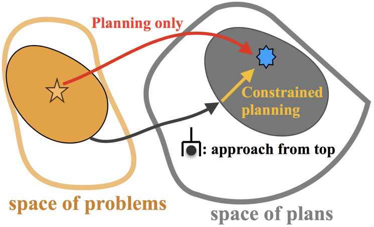
Figure 3: A comparison of search done by a planner without a constraint, and with constraint that forces the planner to find a solution that approaches the target object from the top. The black arrow indicates the work done by a machine learning algorithm, which predicts a constraint, and the yellow arrow indicates the work done by a constrained planner. The gray blob in the space of plans show the reduced search space that satisfies the constraint. The yellow blob in the space of problems indicate the set of problem instances for which there exists a plan that satisfies the top-grasp constraint. The yellow star indicates the given problem instance.

The second challenge is representing problem instances. In most of the TAMP problems that we are contemplating, a manual design of a generic feature representation for predicting constraints is difficult: there are varying numbers and shapes of objects for each problem instance, and some object relations matter for some problem instances but not for others. For instance, in Figure 2 (left), the obstacles on the desk influence how the robot should pick the blue object and the obstacles on the shelf are irrelevant. On the other hand, in Figure 2 (right), the obstacles on the desk are irrelevant.

In light of this, we propose a new type of representation for problem instances, called score-space. In a score-space representation, we represent a problem instance in terms of a vector of the scores for a set of plans on that instance, where each of the plans is computed based on one of a fixed set of promising solution constraints. The intuition is that what matters in a planning problem is how an environment responds to a potential solution, and a good way to predict what solution constraints will work well is to consider how effective other solution constraints have been. Figure 4 shows examples of score-space representations of different TAMP problem instances.

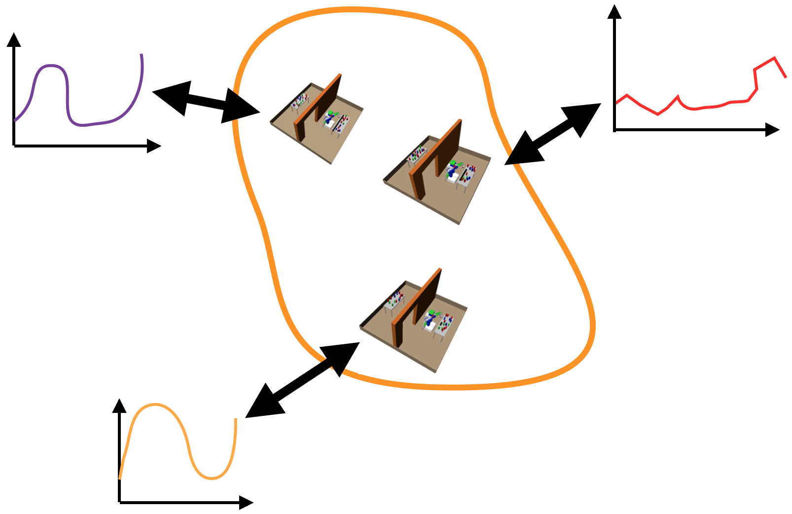
Figure 4: An illustration of a score-space representation of three different problem instances. We assume an one-dimensional constraint for the illustration purpose. The x-axis of a score function represents different values of constraints, and y-axis represents the score of a plan that conforms to a constraint.

The main advantage of the score-space representation is that it gives direct information about similarity between problem instances and solution constraints, without depending on a hand-designed representation. Similar problem instances will have similar patterns of scores on different constraints, and similar constraints will have similar patterns of scores on different problem instances.

For instance, consider again the task in Figure 2. By computing a plan associated with the solution constraint that forces the robot to approach the object from the top and observing that it has a low score, we can learn that it is occluded from above, e.g. by a shelf, and can predict other more appropriate action choices. This information is not biased by the designer’s choice of representation: having learned that approaching the object from the side did not work, a learning algorithm may try to approach the object from the top. Such reasoning is much more difficult when the learning algorithm is forced to reason in terms of a particular representation of the problem, such as poses of obstacles or 2D or 3D images of the scene. The main disadvantage is that the score-space information is computationally expensive to obtain, since it requires computing the plans associated with solution constraints.

This observation brings us to the third challenge of learning to plan, which is how to transfer knowledge from past experience to the current problem instance efficiently. We propose to solve this challenge by using the expectation and correlation of the scores of solution constraints from past problem instances to determine which solution constraint to try next. Our intuition is that the solution constraints that performed well or poorly together are more likely to do so in a new problem instance; for instance, in the previous example for picking an object from a shelf, grasps from the sides would have worked well in most of the problem instances, while grasps from the top or bottom would have worked poorly.

Building on this intuition, we propose an algorithm that directly reasons with the correlation information in the score-space representation of a problem instance. We assume that a score vector that represents a problem instance is distributed according to a Gaussian distribution, and propose box, which is an upper-confidence-bound (UCB) type, experience-based, black-box function-optimization technique (Munos,, 2014; Srinivas et al.,, 2010). box learns to suggests solution constraints based on its belief about the scores of solution constraints, whose prior distribution is computed using scores of constraints in the past planning problem instances, and whose posterior distribution is defined by updating the parameters of the Gaussian distribution using the score feedback from the environment. The overall work-flow is shown in Figure 5.

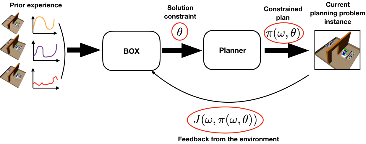
Figure 5: Overall work-flow of BOX. It receives prior experience data in the form of score values, which it uses to compute the prior belief of scores of a current problem instance. It then suggests a constraint to the current problem instance, receives a score, and updates its belief. This process is repeated until we find a solution.

This paper is an improved and extended version of our prior paper (Kim et al.,, 2017). In particular, we make the following additional contributions.

• We prove that our algorithm has a sublinear regret in number of evaluations under certain conditions, using the theoretical results from Bayesian optimization literature (Srinivas et al.,, 2010).

• We propose a new algorithm that reduces the cardinality of an initial set of constraints. It reduces the worst-case evaluation time, the computation time for updating the covariance matrix, and the number of evaluations of a constraint. We add experiments to evaluate the effect of this algorithm.

• We present a new simulation result that requires a significantly longer planning horizon than the ones that we considered in our prior work. Besides the longer horizon, this new domain is especially hard because uniform random sampling of actions would frequently call a motion planner on infeasible problem instances.

In all of the tasks, we show that box can accelerate planning significantly over a basic planner that does not use solution constraints. We also provide a comparison to a sampler that picks solution constraints uniformly at random, and to a state-of-the-art black-box function optimization technique called deterministic optimistic optimization (DOO) (Munos,, 2011) that does not use the score space representation. We find that box  outperforms these other methods. Additional experiments on using a minimal constraint set built using our greedy algorithm indicate that we can almost completely eliminate the covariance matrix inversion time for box, and reduce the total planning time by a factor of 5 for some domains.

2 2. Related work

There is a substantial body of work aimed at improving motion planning performance on new problem instances based on previous experience on similar problem instances (Berenson et al.,, 2012; Hodál and Dvořák,, 2008; Pandya and Hutchinson,, 1992; Jetchev and Toussaint,, 2013; Lien and Lu,, 2009; Phillips et al.,, 2012). The typical approach is to store a large set of solutions to earlier instances so that, when presented with a new problem instance, one can (a) retrieve the most relevant previous solution and (b) adapt it to the new situation. These methods differ in the way that they find the most relevant previous solution and how it is adapted.

Several of these approaches define a similarity metric between problem instances and retrieve solutions based on this metric. For example,  Hodál and Dvořák, (2008) use the distance between the start and goal pairs as the metric, whereas, Pandya and Hutchinson, (1992) based their metric on descriptions of quickly generated low-quality solutions for the current and previous instance. Jetchev and Toussaint, (2013) use a mapping into a task-relevant space and measure similarity in that space, with a learned metric.

Instead of defining solution similarity, Berenson et al., (2012) define relevance of earlier solutions by measuring the degree of constraint violation, for example collision, in the current situation. A related idea is developed by Phillips et al., (2012), where the search graph of past solutions is saved and the search for the current problem instance is biased towards the part of this past graph that is still feasible.

For more complex robotic planning, such as for mobile manipulation in cluttered environments, complete solutions are more difficult to adapt to new problem instances. In particular, the length of the plans is highly variable and they contain both discrete and continuous parameters.

Some earlier approaches have also focused on predicting partial solutions, in the form of a goal state or subgoals, instead of a complete solution. For instance, in the work of Dragan et al., (2011), the objective is to learn from previous examples a classifier (or regressor) that, given a hand-designed feature representation of a planning problem instance, enables choosing a goal that leads to a good locally optimal trajectory. In the approach of Finney et al., (2007), the goal is to learn a model that predicts partial paths or subgoals, from a given parametric representation of a planning problem instance, aimed at enabling a randomized motion planner to navigate through narrow passages.

Several approaches have been proposed for learning representations for robot manipulation skills with varying set of objects (Kroemer and Sukhatme,, 2016, 2017). Specifically, Kroemer and Sukhatme, (2016) proposes a feature selection method that, given a certain basic features of objects in a scene, such as bounding boxes describing their shapes, predicts relevance of each feature for the given task. The relevant features are then used with a low-level robot motion skill represented with a dynamic motion primitive. While this approach is quite general, it still requires a human to design the basic set of features that are relevant for the tasks that the robot will encounter.

Zhu et al., (2017) proposed an approach to learn a representation for learning a complete policy from RGB images. Authors designed an architecture and defined a set of discrete high-level actions that allows an agent to accomplish different tasks. Similar to our approach, they learn a representation from planning experience. However, they learn a complete policy, whereas our approach learns to predict solution constraints. Moreover, their method does not take a robot into account - for manipulation tasks, however, visual representation greatly suffers from occlusion by the end-effectors of the robot. Our score-space representation abstracts away from this problem by directly representing a planning scene with how well the predicted constraints works.

Our approach can be seen as a method for choosing actions from a library; several methods have been proposed for this problem. Dey et al., 2012a propose a method that finds a fixed ordering of the actions in a library that optimizes a user-defined submodular function, for example, the probability that a sequence of candidate grasps will contain a successful one. Unlike our work, this method produces a static list, which does not change across different problem instances. Later, Dey et al., 2012b , generalized the approach by producing an ordered list of classifiers (operating over environment features) that select actions for a given problem instance. This approach again requires hand-designed features for the problem instances.

We formulate our problem as a black-box function optimization problem. In particular, box is motivated by the principle of optimism in the face of uncertainty, which is well surveyed by Munos, (2014). The main idea is to select the most “optimistic” item from the given set of items, by constructing an upper bound on the values of un-evaluated items. The performances of these algorithms are heavily influenced by how the upper-bounds are constructed. For instance, doo (Deterministic Optimistic Optimization), developed by Munos, (2011), first constructs the upper bound on the target function using manually specified semi-metric and a smoothness assumption on the target function. It then chooses the next point to evaluate based on this upper bound in order to balance exploration and exploitation.

Another suite of algorithms for black-box function optimization problems are Bayesian optimization algorithms (Srinivas et al.,, 2010; Wang et al.,, 2017; Snoek et al.,, 2012). In Bayesian optimization, an upper bound of the target function is constructed based on a hand-designed covariance matrix and the Gaussian process assumption. For instance, Srinivas et al., (2010) constructs an upper bound using the confidence interval in an algorithm called Gaussian Process Upper Confidence Bound (gpucb). At each time step, gpucb evaluates the point that has the highest UCB value, observes the function value, and updates the Gaussian process. It returns the query point that resulted in the highest value.

The problem with these approaches is that, in general, they require a human to design a similarity function on problem instances and planning solutions: doo requires a semi-metric, and Bayesian optimization algorithms require a kernel. This introduces human bias in constructing the upper-bounds on the target function, which strongly influences the performance of these algorithms. Moreover, as we have shown in the introduction, designing such a function is not trivial: even a small change in a problem instance may induce a large change in scores.

Rather than relying on a hand-designed similarity function over problem instances and planning solutions, our algorithm, box, operates in a vector space of scores of possible solutions where the correlation information among them can be computed easily.

3 3. Problem Formulation

Our premise is that calling the planner with a solution constraint, although much more efficient than the completely unconstrained problem, takes a significant amount of time and may generate significantly suboptimal plans if the solution constraint used is not a good match for the problem instance. Given a new instance we will call the planner with a fixed number of solution constraints and return the best plan obtained. So, our problem is which solution constraints should be tried, and in what order.

We formulate the problem as a black-box function optimization problem over a discrete space of candidate solution constraints, and use upper bounds constructed from experience on previous problem instances as well as the accumulated experience on this instance to determine which constraint to try next.

Formally, we have a sample space for problem instances, $\Omega$, whose elements $\omega$ are distributed according to $P(\omega)$; a space of possible planning solutions, $\mathcal{X}$; and a space of solution constraints. The plan solution space includes all possible assignments to all of the decision variables, and the solution constraint space includes all possible assignments to a subset of decision variables for the given planning problem. The function $J(\omega,x)$ specifies the score of a solution $x\in\mathcal{X}$ on problem instance $\omega\in\Omega$. We assume a planner $\pi:\Omega\rightarrow\mathcal{X}$ that, given a problem instance $\omega$ can return a solution $\pi(\omega)\in\mathcal{X}$ that is either feasible or near-optimal depending on the nature of the problem. In addition, we assume that, given a solution constraint $\theta$, the planner $\pi$ will return $\pi(\omega,\theta)\in\mathcal{X}$,which is a plan subject to the solution constraint $\theta$; in general this solution will not be optimal (so in general $J(\omega,\pi(\omega))>J(\omega,\pi(\omega,\theta))$), unless $\theta$ was perfectly suited to the problem instance $\omega$, but constraining the plan to satisfy $\theta$ will make it significantly more efficient to compute. With a slight abuse of notation, we will denote $J(\omega,\theta)=J(\omega,\pi(\omega,\theta))$, the evaluation of the solution constraint.

Let $\Theta=\{\theta_{1},\ldots,\theta_{m}\}$ be a set of samples from the space of solution constraints. Now, we formulate our problem as follows: given a “training set” of example problem instances $\omega_{1},\ldots,\omega_{n}$ sampled identically and independently from $P(\omega)$, a discrete set of solution constraints $\hat{\Theta}$, and the score function $J(\cdot,\cdot)$, generate a high-scoring solution to the “test” problem instance $\omega_{n+1}$.

An interesting problem that we do not explicitly address in this paper is how to select the subset of decision variables for specifying constraints $\theta$. In this paper, we manually choose a subset of decision variables as solution constraints, and take the simple approach of solving the training problem instances and then extracting the $\theta$ values corresponding to these chosen constraints. The details of constructing $\Theta$ are provided in Algorithm 2.

3.1 3.1 Black-box function optimization with experience

Instead of designing a problem-dependent representation for problem instances, we represent a problem instance with a vector of scores of solution constraints $\Theta$, where

$$\Phi(\omega)=[J(\omega,\theta_{1}),\cdots,J(\omega,\theta_{m})]$$

$\Phi(\omega)$ here is a random vector that maps a sample from the sample space of problem instances to $\mathbb{R}^{m}$. Using this representation, our training data constructed from $n$ problem instances can be represented with a $n\times m$ matrix

$$\mathbf{D}=\begin{bmatrix}&\Phi(\omega_{1})&\\ &\Phi(\omega_{2})&\\ &\vdots&\\ &\Phi(\omega_{n})&\end{bmatrix}$$

that we call the score matrix. Now, given a new problem instance, $\omega$, our goal is to take advantage of one or more solution constraints in $\Theta$ to find a high scoring plan without evaluating all of solution constraints in $\Theta$. To do this, we will develop a procedure that evaluates $J(\omega,\theta)$ by computing a plan $\pi(\omega,\theta)$ for $k<<m$ values of $\theta$.

We begin by making use of the intuition that some solution constraints (via the plans they generate) are inherently more useful than others, independent of the problem instance. This leads to a naive score-space approach, static, that tries solution constraints in $\Theta$ in a static order according to the empirical mean scores in the $1\times m$ vector computed by

$$\hat{\mu}=\frac{1}{n}\sum_{i=1}^{n}\mathbf{D}_{i}$$ (1)

where $i$ indicates the row of the score matrix, and then returns the highest scoring plan obtained from trying the top $k$ solution constraints.

This simple approach does not take advantage of the fact that there are correlations among the scores of solution constraints across problem instances; that is, the score of a solution constraint that has been already tried on this problem instance can inform us about the scores of other untried but correlated solution constraints. In order to exploit correlation, we assume that the random vector $\Phi$ is distributed according to a multivariate Gaussian distribution, $\mathcal{N}(\mu,\Sigma)$.

Now the score matrix is used to estimate the parameters of the prior distribution of $\Phi$, $\hat{\mu}$ and $\hat{\Sigma}$, where $\hat{\mu}$ is defined in equation 1 and

$$\hat{\Sigma}=\frac{1}{n-1}\sum_{i=1}^{n}(\mathbf{D}_{i}-\hat{\mu})^{T}(\mathbf{D}_{i}-\hat{\mu})$$ (2)

is a $m\times m$ covariance matrix. This prior distribution is updated given evidence about a new problem instance, in the form of score values. Algorithm 1 contains detailed pseudo-code for an algorithm based on these ideas, called box, which stands for Blackbox Optimization with eXperience. It takes as input: $\omega_{n+1}$, the “test” planning problem instance; $\zeta$, a constant governing the magnitude of the exploration; $k$, the number of solution constraints to evaluate; $\Theta$, the set of solution constraints in the training set; $\hat{\mu}$ and $\hat{\Sigma}$, the parameters for the prior distribution of $\Phi(\omega_{n+1})$; $J$, the scoring function; and $\pi$, the planner.

The algorithm first estimates the parameters of the prior distribution. Then, it iterates over solution constraints: first it selects a solution constraint, then it uses the chosen constraint to construct a new plan, and the score of that plan combined with the prior computed from $\mathbf{D}$ is used to determine the next solution constraint to evaluate.

We will use $\Theta_{t}$ to denote the constraints that have been tried up to time $t$, $\bar{\Theta}_{t}=\Theta\setminus\Theta_{t}$ to denote the ones not tried, $\theta^{(t)}$ to denote the index of the solution constraint chosen at time $t$, $x^{(t)}$ to denote the associated plan, $J^{(t)}$ to denote the score of that plan on the given problem instance, and $J^{1:t}$ and $J^{\overline{1:t}}$ to denote the scores of tried and untried solution constraints up to time $t$, respectively.

We will use this constraint notation to refer to corresponding rows and columns in the mean vector and empirical covariance matrix. For instance, at time $t$, we can rearrange the covariance matrix $\hat{\Sigma}$ as

$$\begin{bmatrix}\hat{\Sigma}_{\bar{\Theta}_{t},\bar{\Theta}_{t}}&\hat{\Sigma}_{\bar{\Theta}_{t},\Theta_{t}}\\ \hat{\Sigma}_{\Theta_{t},\bar{\Theta}_{t}}&\hat{\Sigma}_{\Theta_{t},\Theta_{t}}\\ \end{bmatrix}$$

where the subscript represents a set of rows and columns of the matrix $\hat{\Sigma}$. This way, the top-left block matrix is the covariance among untried solution constraints, the top-right and bottom-left represent covariance among tried and untried solution constraints, and the bottom-right represents the covariance among the tried solution constraints.

In line 1 of Algorithm 1, we first estimate the prior distribution of the score function for a new problem instance $\omega_{n+1}$. For the consistency of notations we assume $\hat{\mu}^{(0)}=\hat{\mu}$ and $\hat{\Sigma}^{(0)}=\hat{\Sigma}$. Line 2 selects the next solution constraint to try based on the principle of optimism in the face of uncertainty, by selecting the one with the maximum upper confidence bound (UCB). The next three lines generate a plan using the chosen solution constraint, and then evaluate it. At iteration $t$, given the experience of trying $\Theta_{t}=[\theta^{(1)},\cdots,\theta^{(t)}]$ and getting scores $J^{1:t}:=[J^{(1)},\cdots,J^{(t)}]$, our posterior on the scores of the untried solution constraints, denoted $J^{\overline{1:t}}$, is

$$J^{\overline{1:t}}|J^{1:t}\sim\mathcal{N}(\hat{\mu}^{(t)}_{\bar{\Theta}_{t}},~{}\hat{\Sigma}^{(t)}_{\bar{\Theta}_{t},\bar{\Theta}_{t}})$$

where

$$\hat{\mu}^{(t)}_{\bar{\Theta}_{t}} =\hat{\mu}_{\bar{\Theta}_{t}}+\hat{\Sigma}_{\bar{\Theta}_{t},\Theta_{t}}(\hat{\Sigma}_{\Theta_{t},\Theta_{t}})^{-1}(J^{1:t}-\hat{\mu}_{\Theta_{t}})$$ (3)

$$\hat{\Sigma}^{(t)}_{\bar{\Theta}_{t}} =\hat{\Sigma}_{\bar{\Theta}_{t},\bar{\Theta}_{t}}-\hat{\Sigma}_{\bar{\Theta}_{t},\Theta_{t}}(\hat{\Sigma}_{\Theta_{t},\Theta_{t}})^{-1}\hat{\Sigma}_{\Theta_{t},\bar{\Theta}_{t}}$$

The constant $\zeta$ governs the size of the confidence interval on the scores. We show how the constant can be set through theoretical analysis of regret bounds in the next section. The number of evaluations $k$ should be chosen based on the desired trade-off between computation time and solution quality.

Algorithm 1 BOX($\omega_{n+1},C,k,\Theta,\bf{D},J,\pi$)

1:  Compute $\hat{\mu}^{(0)}$ and $\hat{\Sigma}^{(0)}$ according to Eqns 1 and 2

2:  for  $t=1$ to $k$  do

3:     $\theta^{(t)}=\operatorname{arg\,max}_{i\in\bar{\Theta}_{t}}\hat{\mu}_{i}^{(t-1)}+\zeta\cdot\sqrt{\hat{\Sigma}^{(t-1)}_{ii}}$ // $i^{th}$ entry and $i^{th}$ diagonal entry

4:     $x^{(t)}=\pi(\omega_{n+1},\theta^{(t)})$

5:     $J^{(t)}=J(\omega_{n+1},x^{(t)})$

6:     Compute $\hat{\mu}^{(t)}$ and $\hat{\Sigma}^{(t)}$ using eqn. 3

7:  end for

8:  $t^{*}=\operatorname{arg\,max}_{t\in\{1,\cdots,k\}}J^{(t)}$

9:  return $x^{(t^{*})}$

Algorithm 2 GenerateTrainingData($n,\pi,J,[\omega_{1},\cdots,\omega_{n}]$)

1:  for $\omega$ in $[\omega_{1},\cdots,\omega_{n}]$ do

2:     $x_{i}=\pi(\omega)$ // repeat to get multiple solutions if desired

3:     $\theta_{i}={\it extractConstraint}(x_{i})$ // elements of $\Theta$

4:  end for

5:  for $\omega$ in $[\omega_{1},\cdots,\omega_{n}]$ do

6:     for $\theta$ in $\Theta$ do

7:        $J(\omega,\theta)=J(\omega,\pi(\omega,\theta))$ // elements of $\mathbf{D}$

8:     end for

9:  end for

10:  return $\mathbf{D},\Theta$

In order to create the score matrix $\mathbf{D}$ and solution constraints $\Theta$, we run Algorithm 2. This algorithm takes as input $n$, the number of training problem instances, $\pi$ a planning algorithm that can solve problem instances $\omega_{n+1}$ without additional constraints, $J$, the scoring function for a plan, and $[\omega_{1},\cdots,\omega_{n}]$, a set of training sample problem instances drawn iid from $P(\omega)$. For each problem instance, a solution is generated using $\pi$, and a constraint is extracted from the solution and added to set $\Theta$. The process of extracting constraints is domain-dependent; several examples are illustrated in the experiment section. Each new solution constraint is used to generate a solution $\pi(\omega_{n+1},\theta)$ whose score $J(\omega_{n+1},\theta)$ is stored in the $\mathbf{D}$ matrix.

3.2 3.2 Illustrative examples

We now provide concrete examples of running box on some simple examples. Suppose that our constraint is a set of four different grasps, defined by approach vectors, from the top, left, bottom, and right. Our problem is to plan a collision-free path to grasp a target object. The planner is constrained to use the chosen grasp approach direction to grasp the target object. We arbitrarily choose $\zeta=1.96$ to ensure $95\%$ confidence interval in our experiments, but it could be tuned via cross validation for better performance.

In Figure 6(a), we show an example of a score matrix $\mathbf{D}$ obtained by running Algorithm 2. In this figure, the target object is represented with a black circle, and the blue rectangular objects represent obstacles. We have four training problem instances, shown across the rows of the score matrix, and the four constraints across the columns. For illustrative purposes, we assume a simple binary score function, which outputs one if a constraint is feasible for the given problem instance, and zero otherwise. For example, for the first training problem instance, the top-approaching direction is feasible because there is no obstacle blocking the object in that direction, whereas the left-approaching direction is blocked with an obstacle. For a such binary score function, other prior assumption on the target function, such as Bernoulli distribution, might be more suited; however, we will in general consider score functions that take on real numbers, as we will demonstrate in our experiment section.

In Figure 6(b), we show the result of computing the covariance matrix $\hat{\Sigma}$ using $\mathbf{D}$ and equation 2. In order to understand box more thoroughly, we note some salient correlation information in $\hat{\Sigma}$. First, the top-approaching constraint is positively correlated with the right-approaching direction, whereas it is negatively correlated with the bottom-approaching direction. So, in a new problem instance, if we find that the top-approaching constraint fails, then it will increase the UCB value of the score for the bottom-approaching direction while decreasing the UCB value of the right-approaching direction.

We will illustrate these types of behaviors of using two problem instances shown in Figure 6(c), where the task is to plan a collision-free path to grab the circular magenta object, which is occluded by red obstacles. Clearly, for the problem shown in the first row, the only constraint that would work is the bottom-approaching direction. For the second problem instance, the left-approaching direction would be the only feasible constraint.

Figure 7(a) shows the evolution of UCB values,

$$\hat{\mu}_{i}^{(t)}+\zeta\cdot\sqrt{\hat{\Sigma}_{ii}^{(t)}}$$

of the different constraints we denoted with $i$, as box suggests constraints and receives feedback from the planner and the environment. For example, from the score matrix shown in Figure 6(a), we can see that the average values of the scores for top-,left-, and right-approaching directions are 0.5. The elements in the diagonal of the covariance matrix, which are variances of the scores of different constraints, are approximately 0.33 for these three constraints. These give approximate UCB values of 0.83 for these constraints.

The first plot in Figure 7(a) shows the UCB values when $t=1$. There is a tie among UCB values of the first, second, and the last constraints, so we randomly break the tie and select the second constraint, marked with the red circle. After trying to plan a path with this constraint, we see that it is infeasible. The second plot shows the updated UCB values after observing that the second constraint has a score of zero, using Eqn 3. We see that the UCB values of the first and the last constraint remained unchanged, while the third constraint has increased. This is because the second constraint has zero correlation with the first and last constraints, but has negative correlation with the third constraint, as shown in the Figure 6(b). After this, the last and the first constraints have the same UCB values, and we again randomly break the tie; unfortunately, we chose the fourth one, but from this we can update our UCBs such that all other constraints except the third one are infeasible.

This example is a particularly hard for box, because from our prior experience the third constraint was feasible only 1/4 of the time with the lowest variance. Therefore, our belief about its score was quite low. We now consider the second problem instance in Figure 6(c), which is more favorable. Figure 7(b) shows the evolution of UCB values. At $t=1$, shown in the first plot, we randomly break the tie, and chose the first constraint. After observing this is infeasible, at $t=2$, the UCB value of the fourth constraint, which has positive correlation with the first constraint, also reduces to almost 0. The third constraint was negatively correlated with the first constraint, so its UCB value increased; however, the second constraint, which is the correct constraint for this problem instance, has zero correlation with the first constraint, and its UCB value is higher than the third one even after the update. Hence box ends up choosing the feasible constraint after just a single mistake.

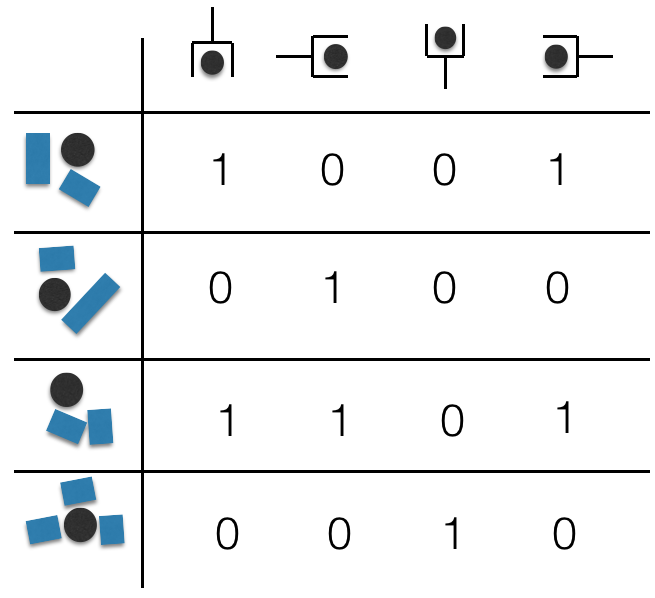
(a) Score matrix, $\mathbf{D}$

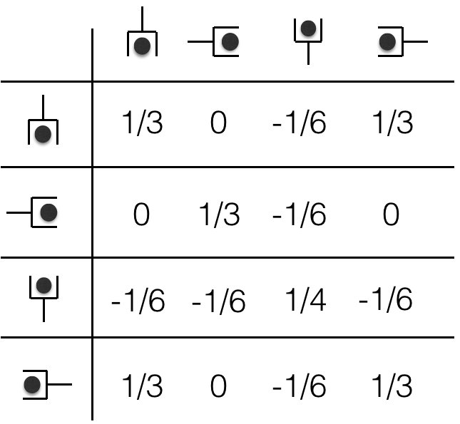
(b) Covariance matrix, $\hat{\Sigma}$

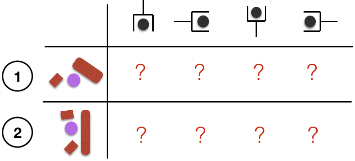
(c) Two new problem instances

Figure 6: Score and covariance matrices for running box, and two new problem instances

(a) Evolution of $\mu$ and UCBs for the first problem instance

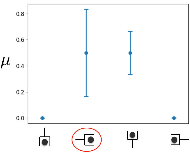
(b) Evolution of $\mu$ and UCBs for the second problem instance

Figure 7: Illustration of how UCBs change as box uses constraints in two different problem instances

4 4. Theoretical analysis of box

In this section, we analyze how the difference between the score of the best constraint in our constraint set $\Theta$ and the score of the best evaluated constraint changes over the iterations of box for a given problem instance $\omega$. We first describe our notation and assumptions.

Since we focus on analyzing box for a new $\omega$, with slight abuse of notation we denote the scores of all the constraints on problem instance $\omega$ as $J=[J(\omega,\theta_{i})]_{i=1}^{m}\in\mathbb{R}^{m}$. We assume that $J\sim\mathcal{N}(\hat{\mu},\hat{\Sigma})$. In other words, this assumption means that there exist a multi-variate Gaussian parameterized by $\hat{\mu}$ and $\hat{\Sigma}$ such that $J$ is a sample drawn from $\mathcal{N}(\hat{\mu},\hat{\Sigma})$. The Gaussian parameters $\hat{\mu}$ and $\hat{\Sigma}$ are defined in in Eq. (1) and Eq. (2). We use the shorthand $\hat{\Sigma}_{A}$ to denote the submatrix $\hat{\Sigma}_{A,A}$ for any subset of constraints $A\subset\Theta$.

We are also going to assume that the diagonal terms of $\hat{\Sigma}$ are bounded, meaning that there exists a constant $c>0$ such that $\hat{\Sigma}_{\theta}<c,\forall\theta\in\Theta$. This assumption limits the variance of the scores of each constraint to be finite. It is a valid assumption in practice because the scores themselves are typically bounded both above and below.

We use regret as the performance measure for box, as typically done in the Bayesian optimization literature. The regret of a black-box function maximization algorithm is defined as the difference between the score of the best constraint selected within the given budget $k$ and the optimal score $J_{\theta_{*}}$ evaluated at the best constraint $\theta_{*}$ in the pre-built finite constraint set $\Theta$; that is

$$r_{k}=J_{\theta_{*}}-\max_{t\in[k]}J^{(t)},$$

where $[k]=\{1,2,\cdots,k\}$ for any positive integer $k\leq m$.

4.0.1 Theoretical results

We first state our main theorem, and then explain its implications and the proof strategy.

Theorem 1.

Pick $\delta\in(0,1)$ and $\sigma>0$ such that $\hat{\Sigma}-\sigma^{2}\bm{I}$ is positive semi-definite. Assume that for $c>0,\ \hat{\Sigma}_{\theta}<c,\ \forall\theta\in\Theta.$ Then with probability at least $1-\delta$, the regret of box with $\zeta=(2\log\frac{1}{\delta})^{\frac{1}{2}}$ satisfies

$$r_{k}\leq 2\sqrt{2\log(\frac{1}{\delta})\left(\frac{2(c-\sigma^{2})\rho_{k}}{k\log(c\sigma^{-2})}+\sigma^{2}\right)},$$

where $\rho_{k}=\max_{A\subseteq\Theta,|A|=k}\frac{1}{2}\log\det(\sigma^{-2}\hat{\Sigma}_{A})$.

On a high level, Theorem 1 shows that boxcan achieve almost zero regret with high probability, under some mild assumptions on the score vector $J$ and its distribution. As long as the score vector $J$ is a sample from $\mathcal{N}(\hat{\mu},\hat{\Sigma})$ and $\hat{\Sigma}$ has decaying spectrum, boxis guaranteed to converge to a constraint whose score is almost the same as the best possible score. We explain in more details below.

In the proof of this theorem, we use a data augmentation trick (Van Dyk and Meng,, 2001) that adds an auxiliary random variable $f\in\mathbb{R}^{m}$ to the graphical model of $J$. Fig. 9 illustrates our problem setup where the generative model is simply $J\sim\mathcal{N}(\hat{\mu},\hat{\Sigma})$. Fig. 9 illustrates the new augmented graphical model and the relation between $f$ and $J$, where the new generative model is,

1. Draw $f\sim\mathcal{N}(\hat{\mu},\hat{\Sigma}-\sigma^{2}\bm{I})$;

2. Draw $J\sim\mathcal{N}(f,\sigma^{2}\bm{I})$.

Notice that we can integrate out $f$ in Fig. 9 and arrive at the same distribution of $J$ as Fig. 9, $J\sim\mathcal{N}(\hat{\mu},\hat{\Sigma})$.

Figure 8: The graphical model of $J$ with Gaussian parameters $\hat{\mu}$ and $\hat{\Sigma}$.

Figure 9: The augmented graphical model of $f$ and $J$ with Gaussian parameters $\hat{\mu}$, $\hat{\Sigma}$ and $\sigma$. The free parameter $\sigma>0$ is chosen such that $\hat{\Sigma}-\sigma^{2}\bm{I}$ is positive semi-definite.

Then, $\rho_{k}$ can be interpreted as the maximum mutual information gain of observations of size $k$ (Srinivas et al.,, 2010):

$$\rho_{k}=\max_{A\subseteq\Theta,|A|=k}I(J_{A};f_{A}).$$

We make the relation clear in Lemma 2. In particular, the mutual information gain is closely related to the predictive variances of the observations.

Lemma 2.

Let $A\subseteq\Theta$, $|A|=k$ and suppose $\hat{\Sigma}-\sigma^{2}\bm{I}$ is positive semi-definite. Then the mutual information between the augmented variable $f_{A}$ and the observation $J_{A}$ satisfy

$$I(f_{A};J_{A})=\frac{1}{2}\log\det(\sigma^{-2}\hat{\Sigma}_{A}),$$

and the information gain of the observations selected by box satisfies

$$I(f_{\Theta_{k}};J_{\Theta_{k}})=\frac{1}{2}\sum_{t=1}^{k}\log(\sigma^{-2}\hat{\Sigma}^{(t-1)}_{\theta^{(t)}}).$$

The exact quantity of $\rho_{k}$ depends on $\hat{\Sigma}$ and how fast the spectrum of $\hat{\Sigma}-\sigma^{2}\bm{I}$ decays. For example, if the off-diagonal terms in $\hat{\Sigma}$ are all 0, there is no correlation between constraints, in which case $\rho_{k}=O(k)$. Theorem 1 shows that the regret is bounded by $O(1)$ which does not decrease as $k$ increases. This is because the scores of all the constraints are independent, so that when some constraints are evaluated, there is no information gained about the scores of other constraints. For robotic domains that we consider, constraints are usually correlated: a constraint on the approach vector of a grasp for an object, for example, would have similar scores across different problem instances if the directions are similar.

Suppose that our original constraint space has dimension $d$; that means, for any constraint $\theta\in\Theta$, it holds that $\theta\in\mathbb{R}^{d}$ and $\Theta\in\mathbb{R}^{m\times d}$. If the covariance matrix satisfies $\hat{\Sigma}\propto\Theta\Theta^{\textrm{T}}+\sigma^{2}\bm{I}$, we have $\rho_{k}=O(d\log(k))$ by (Srinivas et al.,, 2010, Theorem 5). That means our regret bound yields

$$r_{k}\lesssim O\Big{(}\sqrt{\frac{d(\log k)^{2}}{k}}\Big{)}$$

which decreases toward 0 as $k$ increases. We use “$\lesssim$”, approximately less than, to reflect that the bound on $r_{k}$ also depends on a free parameter $\sigma>0$, which can be very small but is always non-zero.

The proof of Theorem 1 depends on the proof of (Srinivas et al.,, 2010, Theorem 3.1), which shows that the cumulative regret of GP-UCB with noisy observations increases sublinearly in the number of evaluations. Srinivas et al., (2010) assume that the diagonal terms of the covariance matrix are all smaller than 1 in their Theorem 3.1. However, in our problem formulation, the score function is noise-free. Moreover, the diagonal terms of our covariance matrix are not bounded by 1. We use the data augmentation trick (Van Dyk and Meng,, 2001) that adds the auxiliary random variable $f$ to introduce artificial noise to our observations. More importantly, we adapt the artificial noise to the scale of the covariance matrix and the number of evaluations. Then, the proof strategy of Srinivas et al. can be reshaped to prove Theorem 1.

The additional artificial noise is critical to the proof of Theorem 1 because it enabled the mutual information to bound the regret. If the artificial noise is 0, the mutual information is not well bounded. The proofs of both Theorem 1 and Lemma 2 can be found in the appendix.

5 5. Constructing a minimal set

In this section, we propose an algorithm for box which tries to reduces the cardinality of $\Theta$ while maintaining important properties, such as the probability that the set will contain a constraint that is applicable to a new problem instance.

We begin with the problem formulation. We wish that, for all problem instances, there is at least one solution in our set. We define a constraint to be feasible for a problem instance if we can find a solution that satisfies it. We will say a constraint covers a problem instance if it is feasible for a problem instance. Given a set of constraints, $\Theta$, we are interested in a minimum cardinality subset of the original constraint set that covers all the problem instances in the training data. We will call such subset a minimal set, and denote it with $\Theta_{min}$.

Out of all the minimal sets, we are interested in those whose probability of success is maximized, so that the set can be applied to a wide range of problem instances. The probability of success is measured by

$$P(\Theta_{min}\text{ succeeds on }\omega)=1-\prod_{\theta\in\Theta_{min}}^{k}(1-p_{\theta})$$

where $k$ is the cardinality of the minimal set, and $p_{\theta}$ is the probability of constraint $\theta_{i}$ in the minimal set being feasible. Notice that $p_{\theta}$ can be approximated by empirical counts of successes divided by the number of problem instances from our training data. We will call a minimal set whose probability of success is maximum a maximally successful minimal set.

Out of all the maximally successful minimal sets, we are interested in those that give maximum information on the values of the scores of other constraints, in order to minimize the number of evaluations. First note that the differential entropy $h$ of the multivariate Gaussian distribution $\mathcal{N}(\mu,\Sigma_{\Theta_{min}})$ over a random vector $\Theta_{min}$ is defined by

$$h(\Theta_{min})=\frac{|\Theta_{min}|}{2}\Big{[}1+\log(2\pi)\Big{]}+\frac{1}{2}\log\det\Sigma_{\Theta_{min}}$$

where $n$ is $|\Theta_{min}|$ and $|\Sigma_{\Theta_{min}}|$ is a determinant of the covariance matrix $\Sigma_{\Theta_{min}}$. Now, using this, we can define the gain function, $g$, which characterizes the information gain for scores of other constraints given an evaluation of a constraint $\theta_{i}$

$$g(\Sigma_{\Theta_{min}},\theta_{i}) =h(\Theta_{min})-h(\Theta_{min}|\theta_{i})$$

$$=\log(|\Sigma_{\Theta_{min}}|)-\log(|\Sigma_{\Theta_{min}|\theta_{i}}|)$$

where $|\Sigma_{\Theta_{min}}|$ is the determinant of the covariance matrix of the minimal set $\Theta_{min}$, and $|\Sigma_{\Theta_{min}|\theta_{i}}|$ is the determinant of the covariance matrix of the minimal set after evaluating the constraint $\theta_{i}$ in $\Theta_{min}$. We will call a maximally successful minimal set that maximizes the gain function an optimally minimal set (OMS) and denote it with $\Theta_{min}^{*}$.

We now formulate the optimally minimal set construction problem as follows. Given an original constraint set $\Theta$, construct a minimal set $\Theta_{min}$ that maximizes the function

$$c(\Theta_{min})=\sum_{\theta\in\Theta_{min}}p_{\theta}+\lambda\cdot g(\Sigma_{\Theta_{min}},\theta)$$

The first term is responsible for maximizing the probability of success for $\Theta_{min}$, and the second term is responsible for maximizing the sum of information gain of each constraint in $\Theta_{min}$. Now the optimally minimal set is defined as

$$\Theta_{min}^{*}=\arg\max_{\Theta_{min}\in 2^{\Theta}}c(\Theta_{min})$$

Clearly, constructing $\Theta_{min}^{*}$ is an NP-complete problem This motivates us to devise a greedy approach that approximately optimizes the function $c$, as described in Algorithm 3.

This algorithm takes as inputs: the experience matrix $\mathbf{D}$, the original constraint set $\Theta$, the approximated parameters of a distribution of score vectors $\hat{\mu}$ and $\hat{\Sigma}$, the number of problem instances $n$ and the number of constraints of the original set $m$, and outputs an approximation of an OMS, $L$.

It operates by progressively constructing a list of constraints, $L$, using the gain function and probability of success of a constraint, which is measured by the mean score function $\mu$.

It begins by first adding the index of the constraint that has the maximum mean score value. Then, it checks the number of problem instances covered by the current list of constraints $L$, using the helper function $nCoveredBy$. It then computes the uncovered problem instance indices, $U$. The algorithm then computes the set of next candidate constraint to add to $L$, $\Theta_{cand}$, by taking the constraint that maximally covers the currently uncovered indices $U$. This maximal coverage step is to ensure that we are minimizing the cardinality of $L$.

From this set, the algorithm updates $\Theta_{cand}$ by considering only those constraints whose mean score is the maximum; it is still a set, since there may be a tie in mean scores. From this set, the algorithm chooses the next constraint to add to $L$, by taking the one that has the maximum gain function value. We update the number of problem instances covered, and repeat until we cover all the problem instances. Lastly the algorithm returns $L$, the set of constraints that approximates the OMS.

Algorithm 3 ConstructOMS($\mathbf{D},\Theta,\hat{\mu},\hat{\Sigma},n,m$)

  $\theta_{next}=\arg\max_{\theta\in\Theta}\mu_{\theta}$

  $L=CreateList(\theta_{next})$

  $C_{\max}=nCoveredBy(L,\{1,\cdots,n\})$

  while  $C_{\max}\neq n$  do

     $U=\{1,\cdots,n\})\setminus CoveredBy(L,\{1,\cdots,n\})$

     $\Theta_{\text{cand}}=\{i|\max_{i\in{1,\cdots,m}}len(CoveredBy(\{L,i\},U))\}$

     $\Theta_{\text{cand}}=\{i|i=\arg\max_{i\in I_{\text{cand}}}\mu_{i}\}$

     $\theta_{next}=\arg\max_{\theta\in\Theta_{\text{cand}}}g(\Sigma_{L},\theta)\}$

     $L=\{L,\theta_{next}\}$

     $C_{\max}=nCoveredBy(L,\{1,\cdots,n\})$

  end while

  return $L$

6 6. Experiments

We demonstrate the effectiveness of score-space algorithms static and box in four robotic planning domains: grasp-selection, grasp-and-base-selection, pick-and-place, and conveyor-belt unloading. Each of these domains has several decision variables and different types of solution constraints. For all the problems, a problem instance varies in the sizes of the objects being manipulated, and the poses of obstacles.

In each of these domains, $\pi(\cdot,\theta)$ finds values of decision variables that are not specified in $\theta$. For example, for the grasp-and-base-selection domain $\pi(\cdot,\theta)$ consists of an IK solver and a path planner, and $\theta$ specifies values such as a robot base pose or a grasp for picking an object that is relevant for achieving a goal. To implement rawplanner, $\pi(\omega)$, we first uniformly sample $\theta$ from their original space, such as $\mathbb{R}^{2}$ for robot base pose, instead of from $\Theta$, and then use $\pi(\omega,\theta)$ with the sampled constraints.

We are interested in both running time and solution quality. We compare score-space algorithms, static and box, with rawplanner as well as two other methods that generate plans by selecting a subset of size $k$ of the solution constraints from $\Theta$ and return the highest scoring one. As previously mentioned, static sequentially selects constraints based on their average score values, without considering their correlation information. rand selects $k$ of the $\theta_{i}$ values at random from $\hat{\Theta}$; doo is an adaptation of doo (Munos,, 2011) to optimization of a black-box function over a discrete set, which is $\Theta$ in our case. Like box, it alternates between evaluating $\theta_{j}$ and constructing upper bounds on the unevaluated $\theta_{i}$ for $k$ rounds. It assumes that the function is Lipschitz continuous with constant $\lambda$, and uses the bound $J^{\omega}(\theta_{i})\leq J^{\omega}(\theta_{j})+\lambda\cdot l(\theta_{i},\theta_{j})$ for some semi-metric $l$, $\lambda\in\mathbb{R}$. We use the Euclidean metric for $l$, and $\lambda=1$.

To show that score-space algorithms can work with different planners, we show results using two different planners: bidirectional RRT with path smoothing implemented in OpenRAVE (Diankov,, 2010), seeded with a fixed randomization seed value, and Trajopt (Schulman et al.,, 2014). In the pick-and-place and conveyor-belt unloading domains, where there is a narrow-passage path planning problem, Trajopt cannot find feasible paths without being given a good initial solution, so we omit it.

In each domain, we report the results using two plots, the first showing the time to find the first feasible solution and the second showing how the solution quality improves as the algorithms are given more time. Each data point on each plot is produced using leave-one-out cross-validation. That is, given a total data set of $n$ problem instances and associated solutions, we report the average of $n$ experiments, in which $n-1$ of the instances are used as training data and the remaining one is used as a test problem instance.

Grasp-selection, grasp-and-base-selection, and pick-and-place problems are satisficing problems in which we are mainly interested in finding a feasible solution. So, a binary score function that specifies the feasibility of a given plan would be sufficient to use box. However, in many problems, we want to find a low-cost plan, rather than just a feasible one, using box’s ability to seek optimal solutions from its library of constraints.

To do this, we design a score function that measures the trajectory length for a feasible plan, and that assigns a large cost if the plan is infeasible in the given problem instance. So, given a plan $\pi(\omega)=(q_{1},\cdots,q_{l})$ where $q_{i}$ denotes a configuration of the robot, our score function is

$$J^{\omega}(x)=\begin{cases}-\sum_{i=1}^{l-1}||q_{i+1}-q_{i}||\text{ if $x$ feasible in $\omega$}\\ d,\text{ otherwise}\end{cases}$$ (4)

where $||\cdot||$ denotes a suitable distance metric between configurations and $d=min(\mathbf{D})-mean(\mathbf{D})$. This is our strategy for finding a domain dependent minimum score for failing to solve a problem. Conveyor-belt unloading domain, on the other hand, is not a satisficing problem: we are interested in maximizing the number of objects that a robot packs into a tight room. The Conveyor-belt unloading domain, is not a satisficing problem: we are interested in maximizing the number of objects that the robot packs into a tight room. Therefore, naturally, our score function is defined as the number of objects packed by a plan $\pi(\omega)$.

6.1 6.1 Grasp-selection domain

Our first problem domain is to find an arm motion to grasp an object that lies randomly either on a desk or a bookshelf, where there also are randomly placed obstacles. Neither the grasp of the object nor the final configuration of the robot is specified, so the complete planning problem includes choosing a grasp, performing inverse kinematics to find a pre-grasp configuration for the chosen grasp, and then solving a motion planning problem to the computed pre-grasp configuration.

A planning problem instance for this domain is defined by an arrangement of several objects on a table. Figure 2 shows two instances of this problem, which are also part of the training data. There are up to 20 obstacles in each problem instance. The robot’s active degrees of freedom (DOF) are its left and right arms, each of which has 7 DOFs, and torso height with 1 DOF, for a total of 15 DOF. $\Theta$ consists of 81 different grasps per each arm, computed using OpenRAVE’s grasp model function. $\Theta$ would be all possible grasps for an object. Notice that since our search space for solution constraints is discrete, rawplanner is equivalent to rand.

Given a solution constraint $\theta$, which is a grasp (pose of robot hand with respect to the object) and an arm to pick the object with, it remains for $\pi(\omega,\theta)$ to find an IK solution and motion plan, which can be expensive, but predicting a good grasp makes the overall process much more efficient. The trajectory of the arm to the pre-grasp configuration, with the base fixed, is scored according to eqn. 4, with a score of $d$ assigned to problem instances and constraints for which no solution is found within a fixed amount of computation.

The experiments were run on a data set of 1800 problem instances. Figure 10(a) compares the time required by each method to find the first feasible plan with RRT as the path planner, and Figure 10(d) compares the time with TrajOpt as the path planner. In both of the plots, we can observe that the score-space algorithms static and box outperform all other algorithms in terms of finding a good solution with a given amount of time. box performs about three times faster than static, showing the advantage of using the correlation information. Compared to doo and rand, box is more than nine times faster. doo does only slightly better than rand, which illustrates that in the space of grasps, the Euclidean metric is not effective.

Figure 11(a) compares the solution quality vs time when RRT is used; figure 11(d) compares the same quantities when TrajOpt is used. Here, the score-space algorithms again outperform the other algorithms, with box outperforming static.

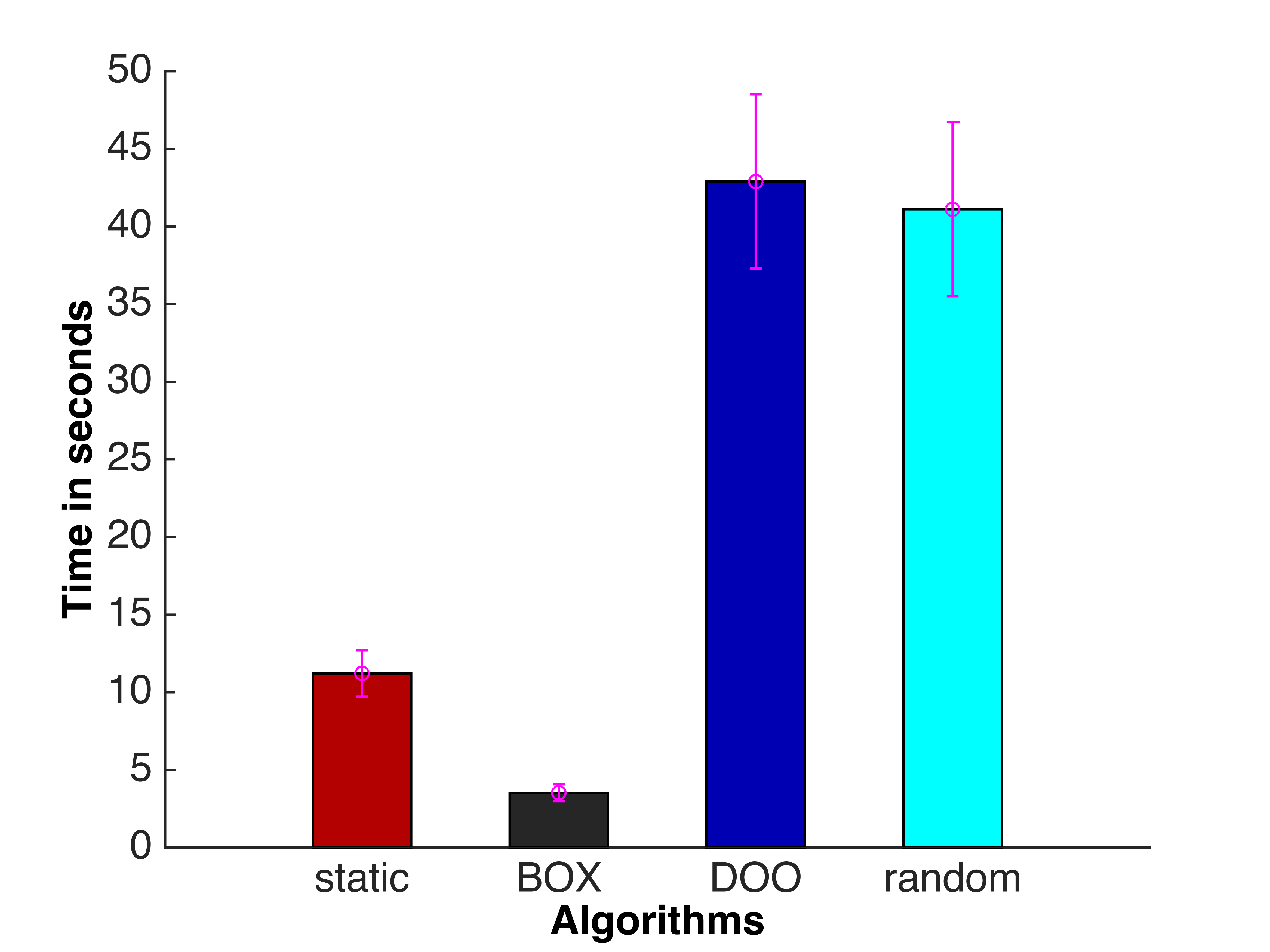
(a) Grasp-selection (RRT)

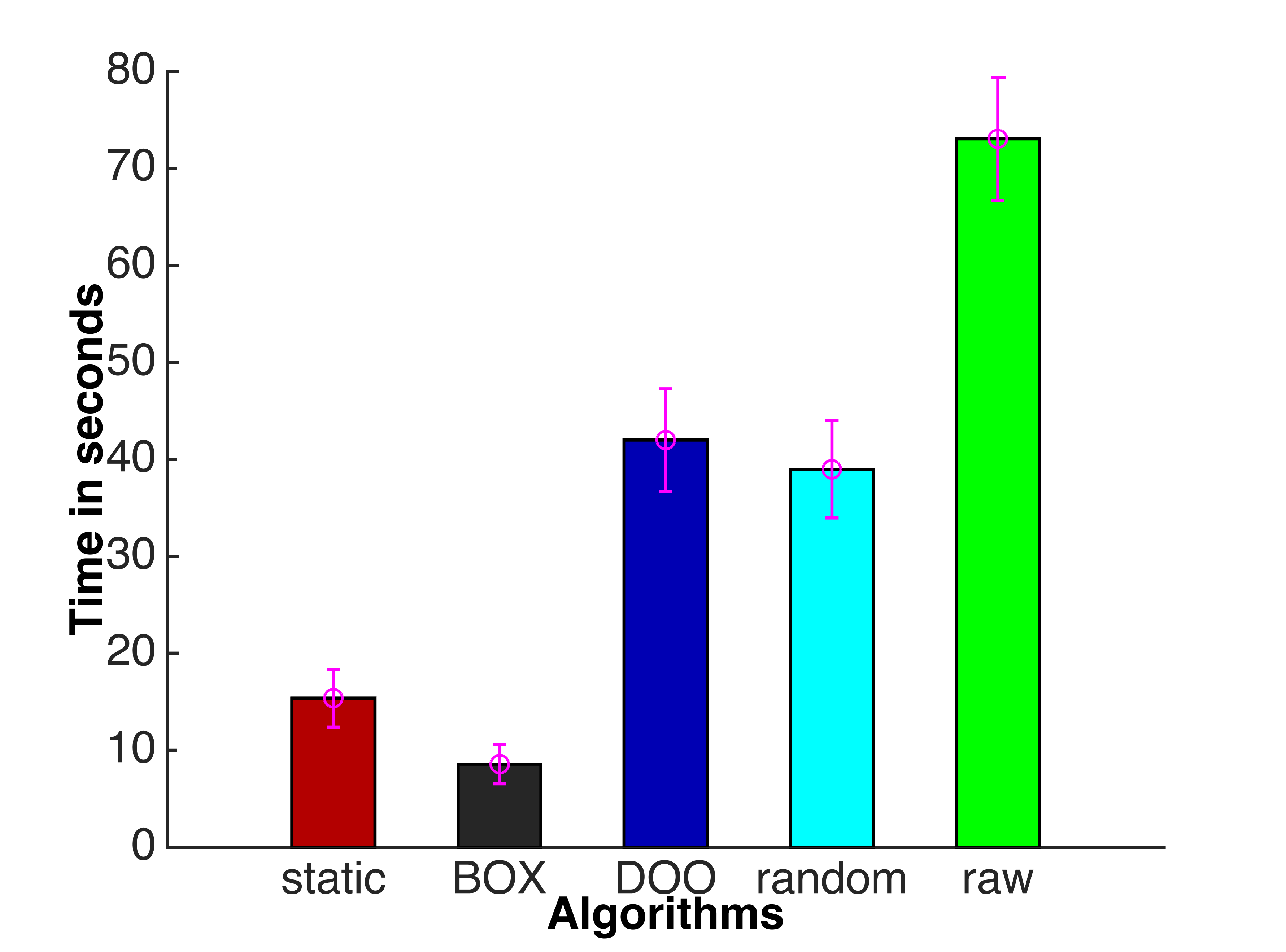
(b) Grasp-and-base selection (RRT)

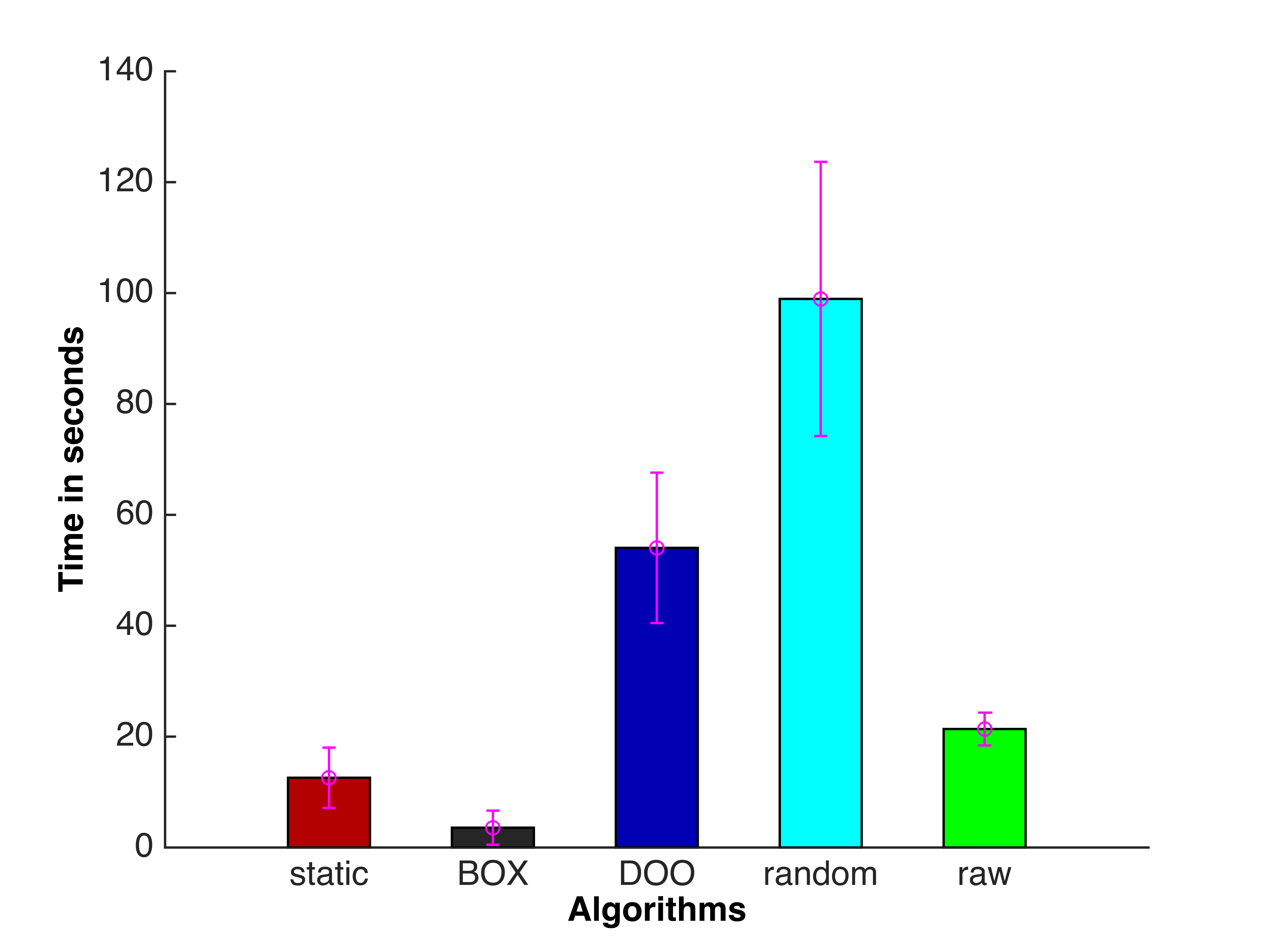
(c) Pick-and-place (RRT)

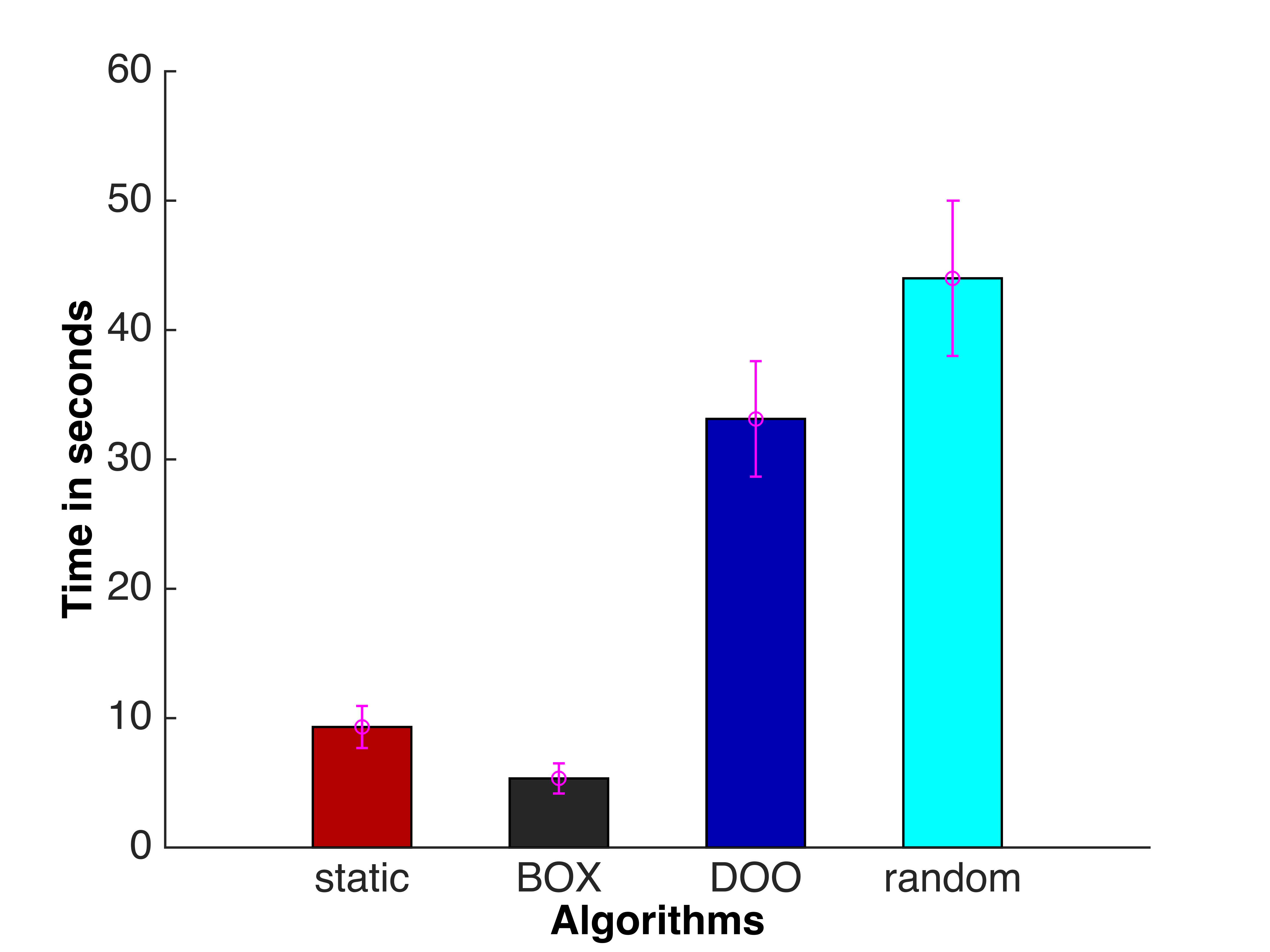
(d) Grasp-selection (TrajOpt)

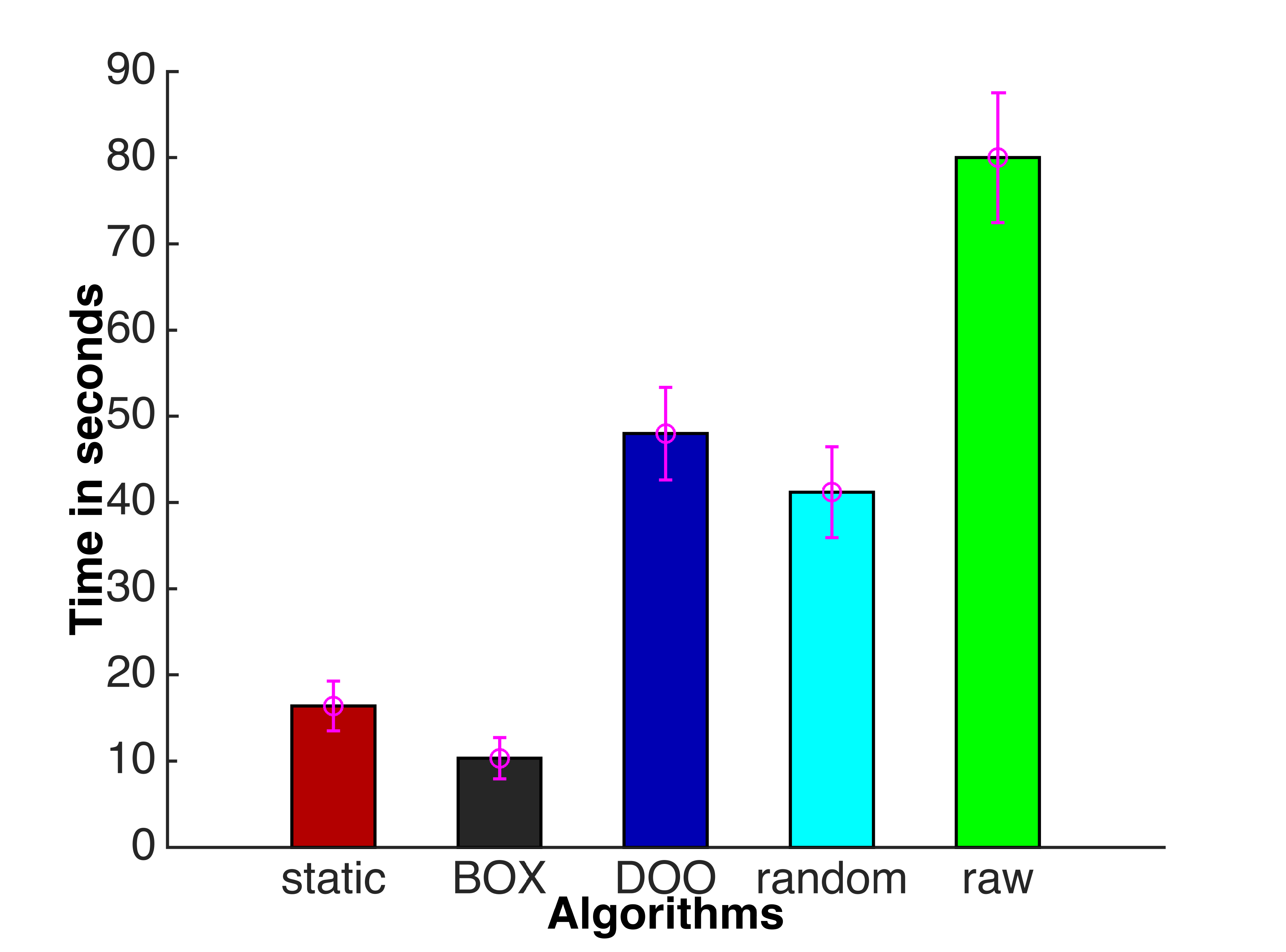
(e) Grasp-and-base selection (TrajOpt)

Figure 10: LOOCV estimate of time to find first feasible solution, for each method in different domains. Whiskers indicate 95% confidence interval on mean. The top row uses RRT and the bottom row uses TrajOpt

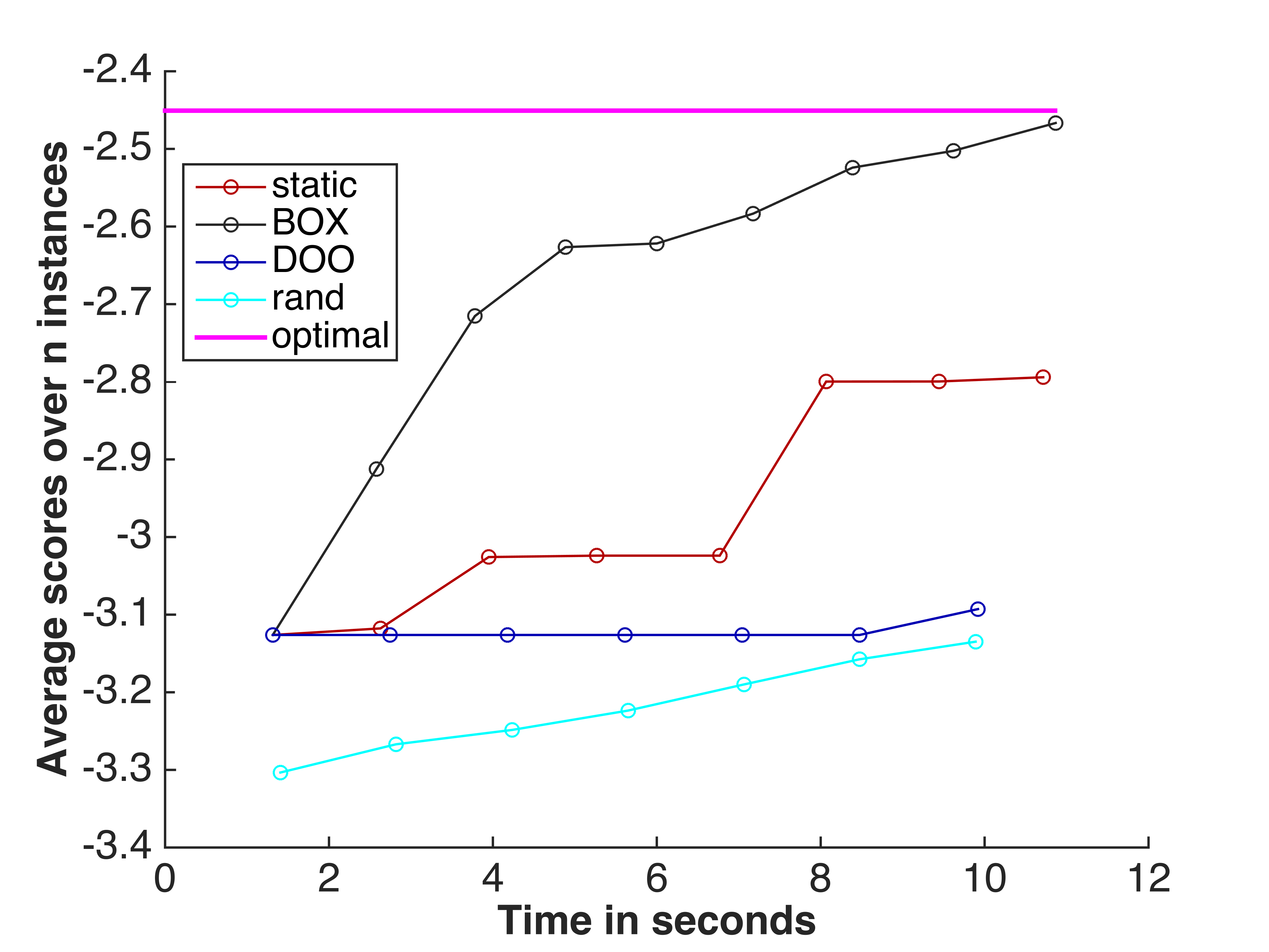
(a) Grasp-selection (RRT)

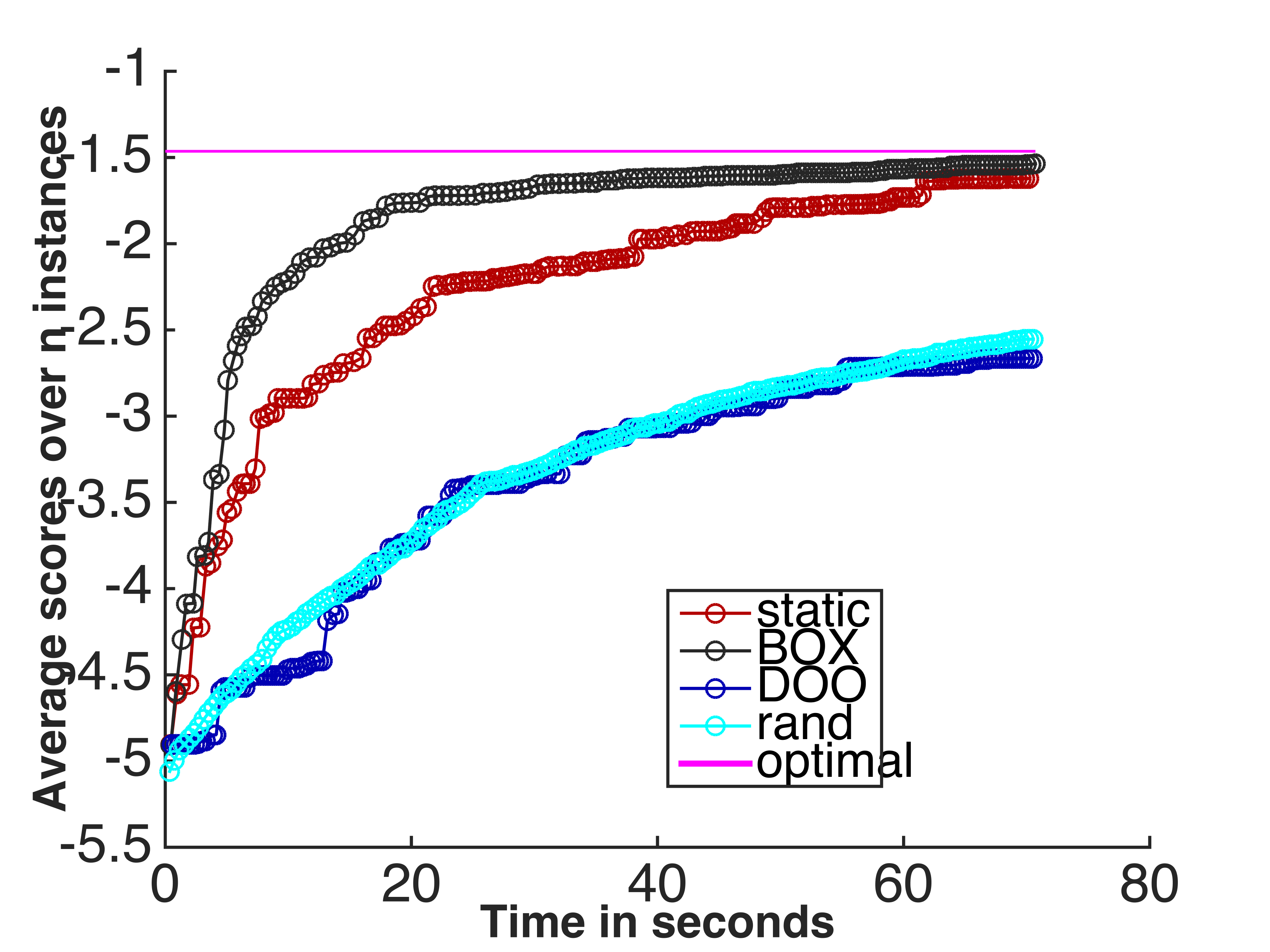
(b) Grasp-and-base selection (RRT)

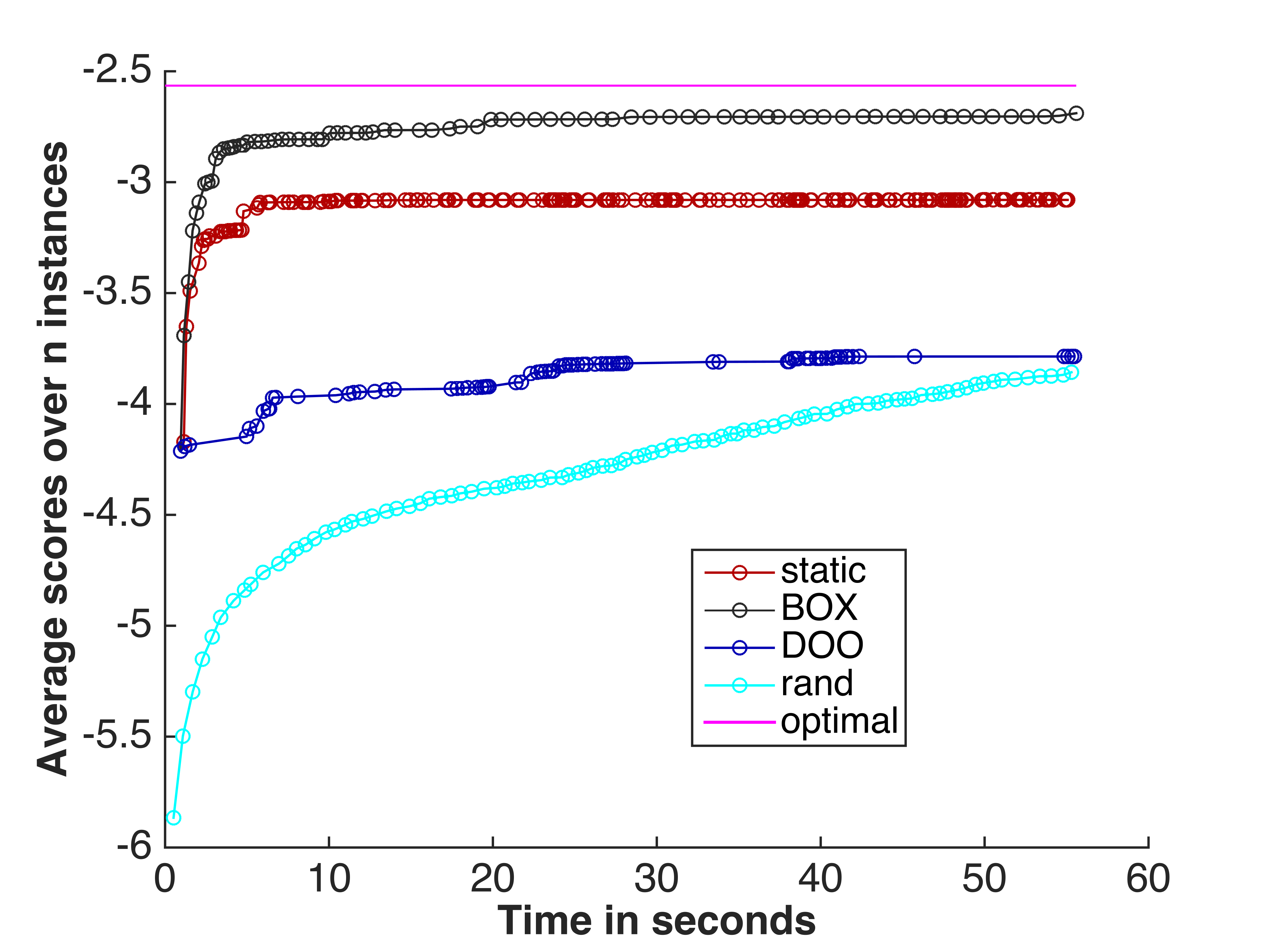
(c) Pick-and-place (RRT)

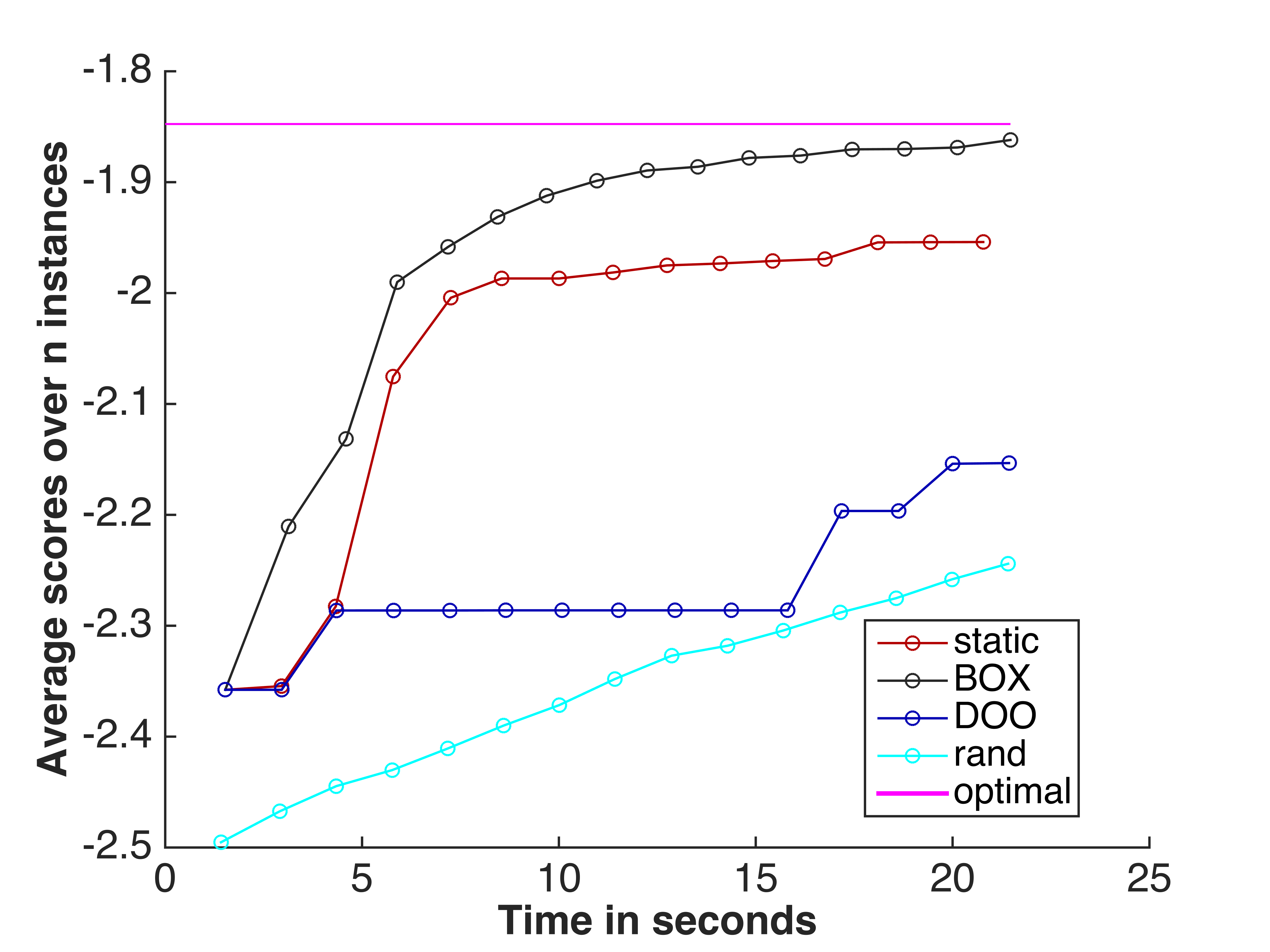
(d) Grasp-selection (TrajOpt)

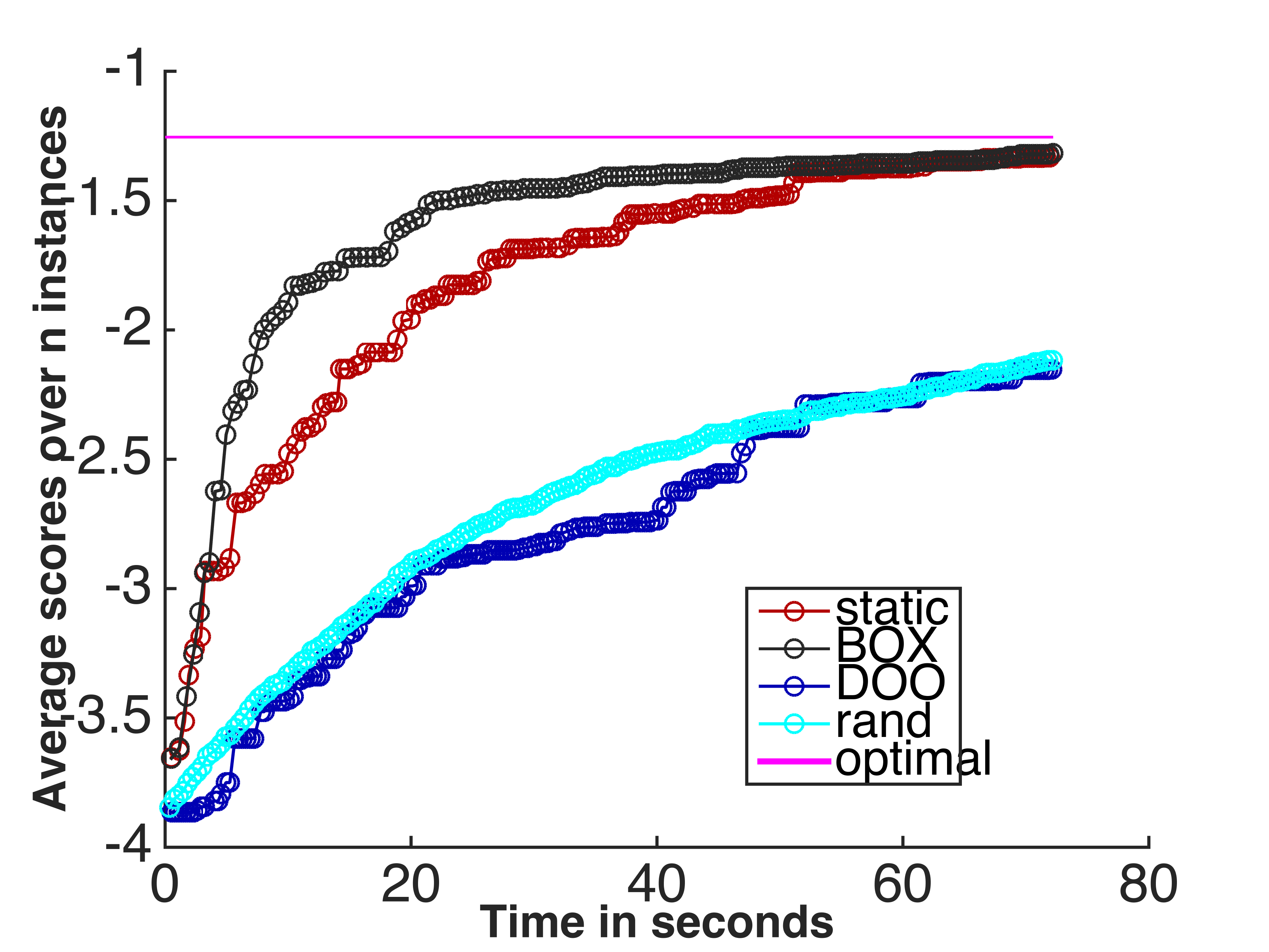
(e) Grasp-and-base (TrajOpt)

Figure 11: Solution score versus run time for different algorithms in various domains. The time axis goes until the first algorithm reaches 95% of the optimal score, marked with magenta. This optimal line is obtained by taking the $\theta$ from $\Theta$ that achieved maximum score for each problem instance. The top row uses RRT and the bottom row uses TrajOpt.

6.2 6.2 Grasp-and-base selection domain

In this experiment, we evaluate how the score-space algorithms perform when we construct the matrix $\Theta$ by sampling from a continuous space. Here, the robot needs to search for a base configuration, a left arm pre-grasp configuration, and a feasible path between these configurations to pick an object.

A planning problem instance is again defined by the arrangement of objects. Figure 12 shows three different training problem instances. We have 20 rectangular boxes as obstacles, all resting on the two tables both of which remain fixed in all instances. For each of the red obstacles and the blue target object, the $(x,y)$ location and orientation in the plane of the table are randomly chosen subject to the constraint that they are not in collision. It is possible that the problem instances will be infeasible (the target object is too occluded or kinematically unreachable by the robot). The robot always starts at the same initial configuration.

The robot’s active DOFs include its base configuration, torso height, and left arm configuration, for a total of 11 DOF. A solution constraint for this domain consists of the robot base configuration to pick the target object, $(x,y,\psi)$, where $\psi$ is an orientation of the robot, as well as one of 81 grasps from the previous section.

Figure 12: Three instances in which the robot must select base configuration, grasp, and paths, to pick the target object (blue). The poses of the objects are randomly varied between instances.

The solution constraints in this case are the grasp $g$, and the base configuration $k$. Given a planning problem instance with no constraints, the rawplanner for this domain performs three sampling procedures, using a uniform random sampler, backtracking among them as needed to find a feasible solution:

1. Sample a base configuration, $k=(x,y,\psi)$, from a circular region of free configuration space, with radius equal to the length of the robot’s arm, centered at the location of the object.

2. Sample, without replacement, from the 81 grasps until a legal one is found, i.e. one for which there is an IK solution in which the robot is holding the target object using that grasp in a collision-free configuration.

3. Use bidirectional RRT or TrajOpt to find a path for the arm and torso between the configurations found in steps 1 and 2.

We assume that the configuration from step 1 is reachable from the initial configuration. To extract a solution constraint from the resulting plan, we simply return the base configuration from step 1 and the grasp from step 2.

Unlike rawplanner, which has to search for $k$ and $g$, $\pi(\omega,\theta)$ simply solves the inverse kinematics and motion planning problems as in the previous example. The trajectory of the arm to the pre-grasp configuration, with the base fixed according to the constraint, is scored according to equation 4, with a score of $d$ assigned to problem instances and constraints for which no feasible solution is found within a fixed number of iterations of the RRT. The experiments were run on a data set of 1000 problem instances. The set $\Theta$ contained 1000 pairs of grasp and robot base configuration, each extracted from a different problem instance.

Figures 10(b) and 10(e) show the time required by each method to find the first feasible plan, using RRT and TrajOpt as the planner. The score-space algorithms perform orders of magnitude better than the other algorithms, with box again outperforming static. doo and rand do provide some advantage by using previously stored solution constraints compared to rawplanner. rawplanner has to sample in the continuous space of base configurations and check whether an IK solution and feasible path exist by running IK and path planning. This causes a significant increase in time to find a solution.

Figure 11(b) compares the solution quality vs time when RRT is used and Figure 11(e) compares the same quantities when TrajOpt is used. Again, the score-space approaches outperform all other methods, with box performing better than static, by using the correlation information from the score space. doo and rand perform similarly, mainly because that simple Euclidean distance is not effective for the hybrid space of base configuration and grasps.

6.3 6.3 Pick-and-place domain

In this experiment, with problem instances as shown in figure 13, we introduce solution constraints involving the placements of objects. Here, the robot needs to pick a large object (shown in black) up off of a table in one room, carry it through a narrow door, and place the object on a table. The initial poses of the target object and the robot are fixed, but problem instances vary in terms of the initial poses of 28 obstacles on both the starting and final tables, which are chosen uniformly at random on the table-tops subject to non-collision constraints, and the length of the target object, which is chosen at random from three fixed sizes.

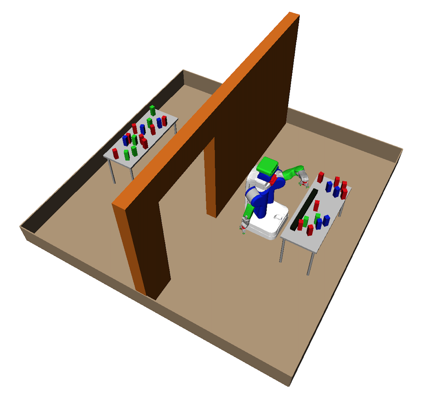
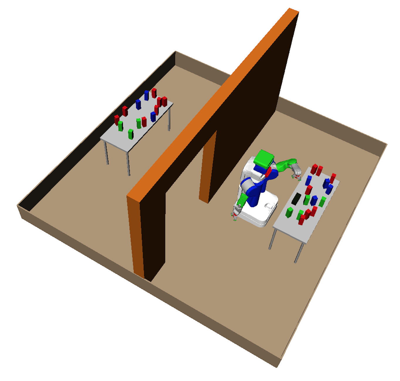
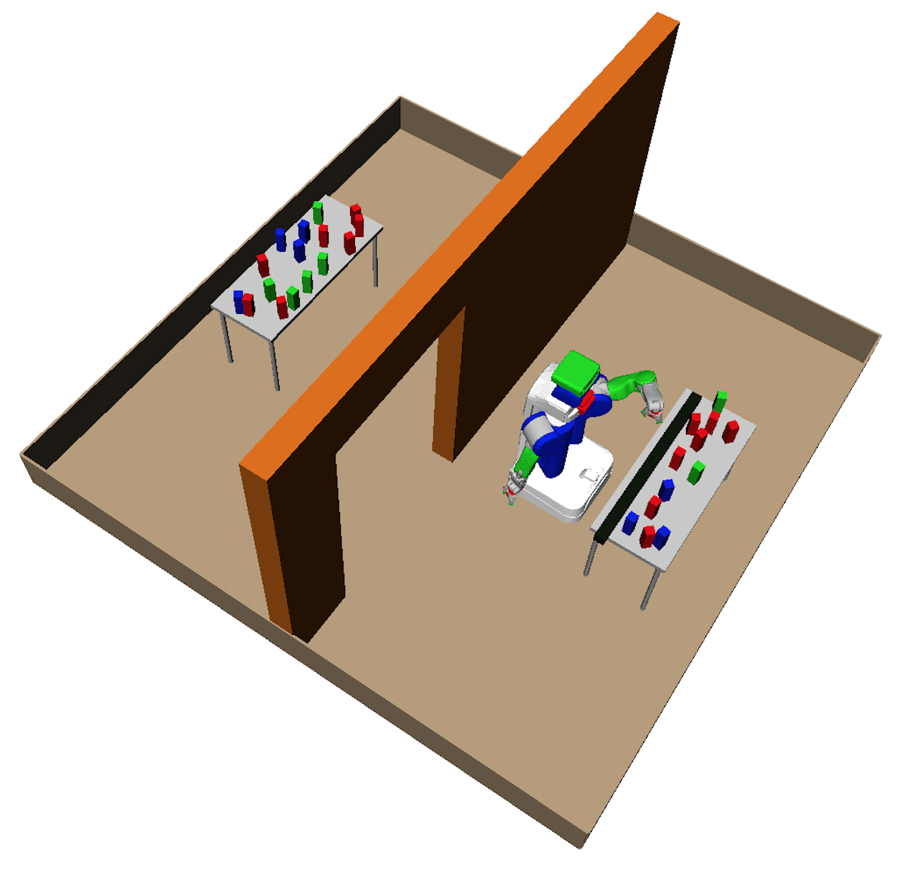
Figure 13: Three problem instances from the pick-and-place domain. The robot’s initial configuration and the black object’s initial pose are fixed across different planning scenes, but other objects’ poses and the black object’s length vary.

The robot’s active DOFs are the same 11 DOFs as in the previous problem domain. The solution constraints in this domain consists of grasp $g$ to pick the object, $o$, the placement pose of the object on the table in the back room, $k_{b}$, the pre-placement base configuration of the robot for placing the object at pose $o$, and $k_{sg}$, the subgoal base configuration for path planning through the narrow passage to $k_{b}$ from the initial configuration.

Given a problem instance with no constraint, rawplanner performs six sampling procedures, similarly to the previous domain, using a uniform random sampler:

1. Sample a grasp $g$, without replacement, from the 81 grasps until a legal one is found.

2. Plan a path for the arm and torso to the pre-grasp configuration found in step 1. If none is found, choose another grasp.

3. Sample a collision-free object pose $o$ on the table in the other room.

4. Sample $k_{b}$, the pre-placement base configuration, from a circular region of free configuration space around $o$, with radius equal to the length of the robot’s arms. If none is found, go back to the previous step.

5. Plan a path from the initial configuration to $k_{b}$. If none is found, go back to the previous step.

6. Plan a path from $k_{b}$ to a place configuration for putting the object down at $o$. If none is found, go back to the previous step.

In contrast, given a solution constraint, $\pi(\omega,\theta)$ simply solves for inverse kinematics and path plans.

The experiments were run on a data set of $1500$ problem instances, with 500 instances per rod size. The set $\hat{\Theta}$ contained 1000 tuples of solution-constraint values, obtained first by running Algorithm 2 and then randomly subsampling them to reduce the size to 1000.

Figure 10(c) shows the time required by each method to find the first feasible plan. Again, the score-space algorithms significantly outperform the other algorithms and box outperforms static. One noticeable difference between this domain and the previous two is that an ineffective solution constraint takes a long time to evaluate, because computing a path plan or IK solution for an infeasible constraint is computationally expensive. This is evident in performance of rand and doo which perform worse than rawplanner as they tend to choose solution constraints that are infeasible and expensive to evaluate.

Figure 11(c) shows the average solution score as a function of computation time. The graphs show a similar trend as in the previous experiments, with score-space algorithms outperfoming the other algorithms, and box performing better than static. The fact that this domain requires a significant amount of time to try an ineffective solution constraint is again evident in doo’s plot, where consecutive dots have a large gap between them. box and static are able to avoid this problem by exploiting the score-space information.

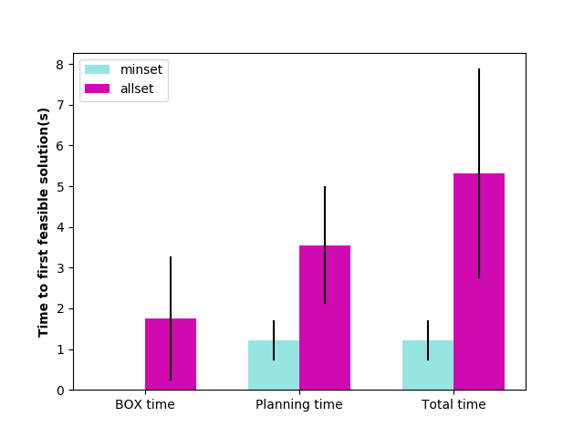
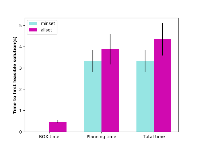
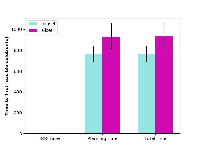
Figure 14: A comparison of time to find a first feasible solution for grasp-and-base-selection domain (left), pick-and-place domain (middle), and conveyor belt domain (right). minset refers to running box with the constraint set found by Algorithm 3, and allset refers to running BOX using the original set $\Theta$. box time refers to time spent (mostly) inverting the covariance matrix, and planning time refers to time spent on planning using chosen constraints.

6.4 6.4 Conveyor belt unloading domain

In this domain, the robot has to manipulate box-shaped objects using two-handed grasps. The robot’s objective is to receive five box-shaped objects with various sizes from a conveyor belt and pack them into a room with a narrow entrance. A problem instance is defined by the shapes and order of the objects that arrive on the conveyor belt. Examples of problem instances are shown in Figure 15, and a solved problem instance is shown in Figure 16.

The robot must make a plan for handling all the boxes, including a grasp for each box, a placement for it in the room, and all of the robot trajectories. The initial base configuration is always fixed at the conveyor belt. After it decides the object placement, which uniquely determines the robot base configuration, a call to an RRT is made to find, if possible, a collision-free path from its fixed initial configuration at the conveyor belt to the selected placement configuration. The robot cannot move an object once it has placed it.

The three previous problems involve an infinite branching factor, but a relatively shorter planning horizon than this problem: if we assume that a call to a motion planner is a “step” in our plan, since we are using it as a primitive planner, the grasp-selection domain has a horizon of one, the grasp-base-selection domain is a has a horizon of two (for base planning and arm planning for picking an object), and the pick-and-place domain has a horizon of three (for picking an object, moving robot’s base, and then to place the held object). The conveyor-belt domain requires a horizon of ten, for picking and placing five objects in total.

Further, this domain is particularly challenging compared to the previous experiments for two reasons. First, the robot is operating in an environment with tight free-space, in which there may or may not be a collision-free path from one robot configuration to another. If the object placements are not carefully chosen, calls to the motion planner will be extremely expensive, either because they are infeasible and will have to run until a time-out is reached, or because the tolerances are tight and so even if the problem is feasible, it may run for a long time or time out. Second, they contain a large volume of “dead-end” states that require the task-level planner to backtrack. For example, if the planner greedily places early objects near the door, then it will eventually find that it is infeasible to place the rest of the objects and will have to backtrack to find different placements of those objects.

As mentioned, we have a significantly longer horizon planning problem than the previous domains. Therefore, we use graph-search with the sampled operators as our rawplanner. It proceeds as follows:

1. Place the root node on the search agenda.

2. Pop the node from the agenda with the lowest heuristic value (estimated cost to reach the goal)

3. Expand the popped node by generating three operator instances by sampling their parameters, and add their successor states on the search agenda.

4. If the popped node is a root node, add it back to the queue after expansion

5. If at the current node we cannot sample any feasible operators, then we discard the node and continue with the next node in the agenda.

6. Go to step 2 and repeat until we arrive at a goal state.

We have two operators: pick and place. To sample parameters for the pick operation, the raw planner rawplanner executes the following steps:

1. Sample a collision-free base configuration, $(x,y,\psi)$, uniformly from a circular region of free configuration space, with radius equal to the length of the robot’s arm, centered at the location of the object, using a uniform sampler.

2. With the base configuration fixed at $(x,y,\psi)$, sample $(d,h,\gamma)$, where $d$ and $h$ are in the range $[0.5,1]$, and $\gamma$ is in the range $[\frac{\pi}{4},\pi]$, uniformly. If an inverse kinematics (IK) solution exists for both arms for this grasp, proceed to step 3, otherwise restart.

3. A linear path from the current arm configuration to the IK solution found in step 2 is planned.

At each stage, if a collision is detected, this means that the sampled parameters are infeasible, so sampling proceeds from the step 1

We assume that the conveyor belt drops objects into the same pose, and the robot can always reach them from its initial configuration near the conveyor belt, so we omit step 3. From a state in which the robot is holding an object, it can place it at a feasible location in a particular region. To sample parameters for place, rawplanner executes following steps:

1. Sample a collision-free base configuration, $(x,y,\psi)$, uniformly from a desired region $R$.

2. Use bidirectional RRT from the current robot base configuration to $(x,y,\psi)$.

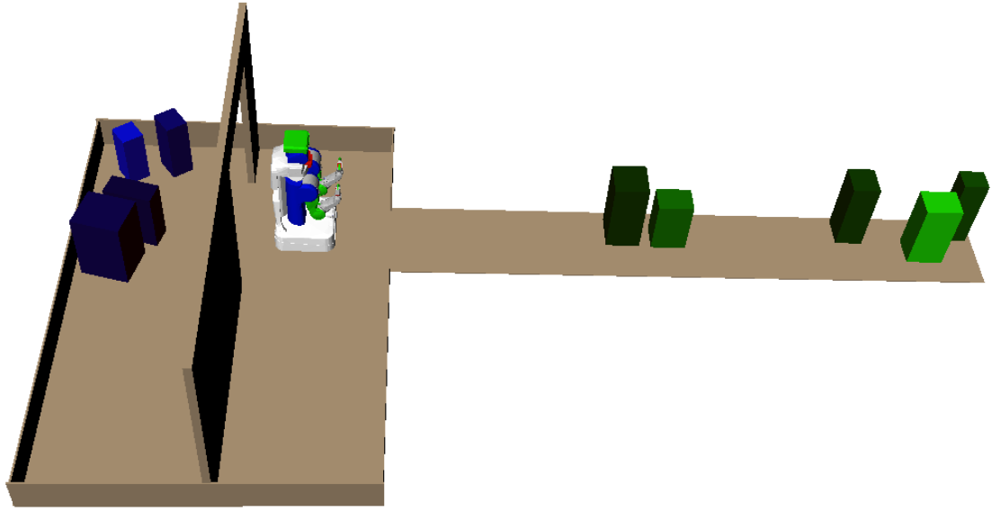
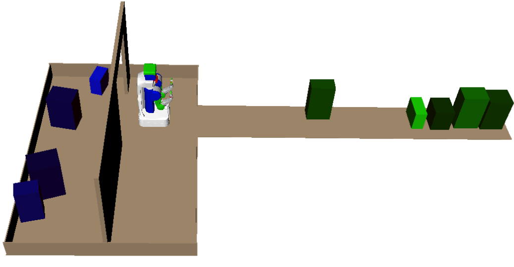
Figure 15: Two instances of the conveyor belt domain

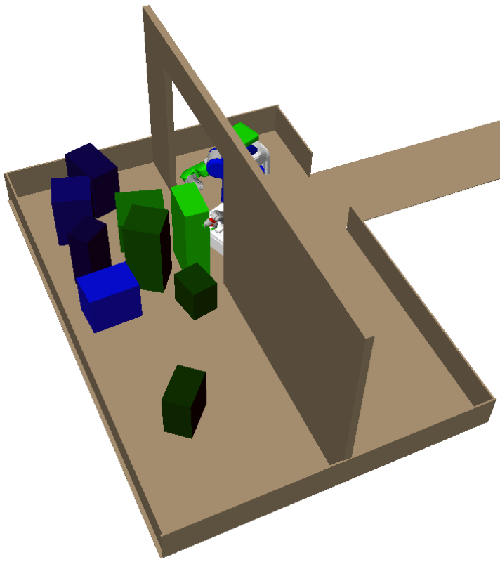
Figure 16: A solution for the conveyor belt domain

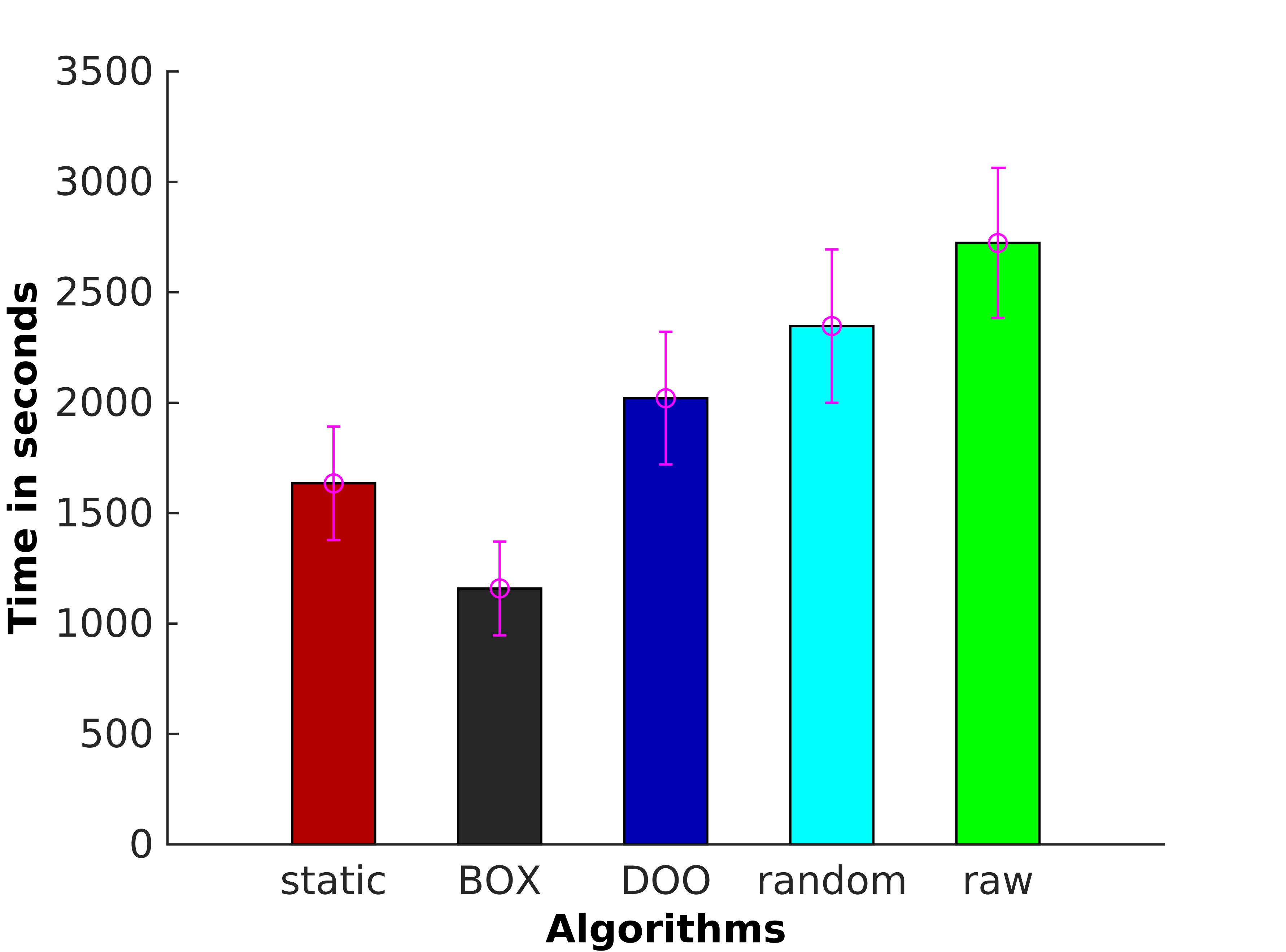
(a) Time to pack four objects for the conveyor belt domain using RRT

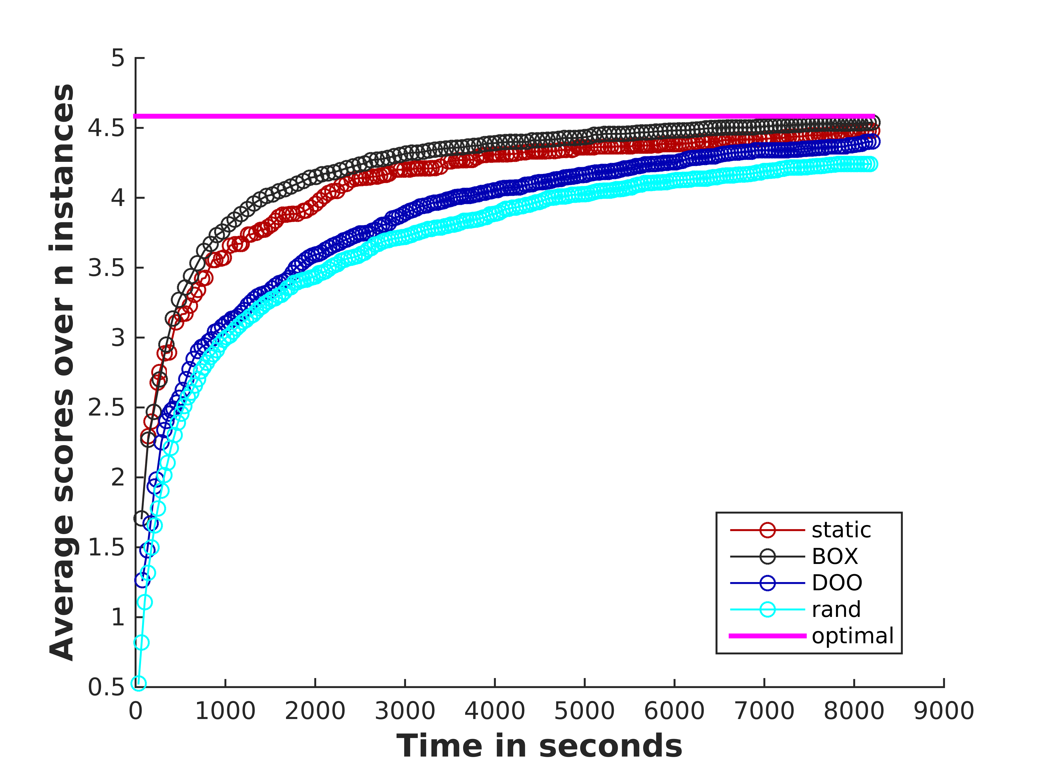
(b) Solution score vs run time for the conveyor belt domain using RRT

Figure 17: LOOCV estimates of different performance metrics for the conveyor belt domain

The experiments were run on a dataset of 468 problem instances. The solution constraints in this domain consists of the base configuration for the pick operator, and the base configuration for place operator. The size of $\Theta$ was 400, obtained by running Algorithm 2 on total of 468 problem instances and then randomly subsampling them to reduce the size to 400.

Figure 17(a) shows the time required by each method to pack four objects. Again, the score-space algorithms significantly outperform the other algorithms and box outperforms static. In this domain, each evaluation of a constraint is significantly longer than in the previous domains, because trying a constraint involves calls to an RRT up to ten times, some of which may be an infeasible motion planning problem. We also notice that doo does not perform as badly as in the previous domains, because the constraints are defined on the base poses of robots, in which Euclidean distance is a reasonable metric.

Figure 11(c) shows the average solution score as a function of computation time. The graphs show a similar trend as in the previous experiments, with score-space algorithms outperfoming the other algorithms, and box performing better than static. Compared to the previous domains, the difference between box and static is much smaller. This is because in this domain, any strategy that packs objects inside first and then gradually towards the narrow entrance will tend to have high scores. Therefore, static, which uses the mean of the scores, works reasonably well, although box generally does better.

6.5 6.5 Experiments with optimally minimal set

The purpose of this experiment is to verify our hypothesis that reducing the size of the constraint set reduces the time for matrix inversion involved in updating the mean and covariance matrix in box, as well as the time to find the first feasible solution. We test Algorithm 3 in the first three problems previously solved using box with full constraints, the grasp-and-base-selection domain, pick-and-place domain, and conveyor-belt domain, and provide comparisons. We omit the grasp-selection domain because it already has a small constraint set of size 162, compared to 1500,1000, and 500 for the other three domains.

Using Algorithm 3, we were able to reduce the constraint set size significantly. For the grasp-and-base-selection domain, the algorithm reduced it to 41 from 1500 for the pick-and-place domain it reduced the constraint set size to 69 from 1000, and for the conveyor-belt domain it reduced from 500 to 76.

Figure 14 shows the times to find a first-feasible solution for these domains using the reduced constraint set. As we can see, it reduces both planning time and box time, which confirms our hypothesis. In fact, in all of the domains, it reduced the box time, which mostly consists of covariance matrix inversion time, to almost zero. In terms of reduction in planning times, the reduction was approximately a factor of around 3 for the grasp-and-base-selection domain. The reduction is smaller in the pick-and-place and conveyor belt domains, although there is a notable reduction. The reason that the reduction is smaller in these two domains is because there generally is a smaller reduction in variance of scores of other constraints compared to the grasp-and-base-selection domain when one constraint is evaluated.

7 7. Discussion and future work

In this paper, we proposed an algorithm for learning to guide a planner for task-and-motion planning problems by addressing three important questions: what to predict, how to represent a planning problem instance, and how to transfer planning knowledge from one instance to another.

In order to trade-off between the burden on the learning algorithm and the planner, we proposed to predict constraints on the planning process rather than a complete solution. To eliminate the bias and cumbersome feature design, we introduced a score-space representation, in which we construct a representation of a problem instance using a set of scores of plans that satisfy a pre-built discrete set of constraints on-line. To transfer knowledge, we proposed box, an algorithm that tries to both accurately construct a score-space representation of the given problem instance and choosing a constraint to try next from the given set.

As an extension to our original work, we also proposed an approach for reducing the constraint-set size. This is motivated by the fact that box requires inverting a matrix, which gets larger as the size of the constraint-set increases. This algorithm effectively reduced the constraint-set size, which lead to reduced covariance matrix inversion time and reduced number of evaluations of constraints. We demonstrated effectiveness of these algorithms in four challenging TAMP domains. We now discuss limitations of the current approach and future work.

7.1 7.1 Fixed plan skeletons

In this work, we focused on TAMP problems such that even for a fixed sequence of operators, also known as plan skeletons (Lozano-Pérez and Kaelbling,, 2014), the planner would yield a solution even for different problem instances. For example for the grasp-and-base selection domain, the sequence MoveBase,Pick was sufficient, and for the pick-and-place domain the sequence Pick,MoveBase,Place was sufficient for different problem instances. As noted by Lozano-Pérez and Kaelbling, (2014), the same plan skeleton can solve a large number of problem instances for some TAMP problems.

However, there are more general TAMP problems in which a fixed plan skeleton would not work. For example, consider the problem of making a cup of coffee, where a problem instance is defined by the number of spoons of sugar to put in. For such variation in problem instances, we would need different plan skeletons depending on the request.

To deal with this limitation, we are currently working on learning high-level constraints that constrains the search space of plan skeletons from planning experience. Since the number of plan skeletons is discrete, if we can find a good set of constraints that reduces the space of plan skeletons to a small but promising set, then we can construct $\Theta$ for each skeleton, and then use box appropriately.

7.2 7.2 Discrete constraints

To make use of the correlation information among scores of constraints, our approach builds a discrete set of constraints and evaluates them on training problem instances during the training phase. For some applications, however, finding a solution that conforms to one of the constraints from a selected discrete set might be insufficient to cope with changes in problem instances. For instance, consider the task of moving objects to clear a path to the target object. Depending on the arrangement of moveable obstacles, we would need different object placements each time, and covering all possible such placements in a discrete set would be difficult.

For this problem, we are currently looking into generative models for generating promising constraints from the original space $\Theta$. The idea is to use the recent advancement in generative model learning (Goodfellow et al.,, 2014) to generate constraints with high scores, by training a generative model for constraints using successful plans. The main challenge would be how to incorporate score information appropriately to generative adversarial network.

Appendix A Appendix A: Proofs in Section 4

We first prove Lemma 2.

Proof.

(Lemma 2). Mutual information can be expressed as the difference between entropies,

$$I(f_{A};J_{A}) =H(J_{A})-H(J_{A}\mid f_{A})$$

$$=\frac{1}{2}\log\det(2\pi e\hat{\Sigma}_{A})-\frac{1}{2}\log\det(2\pi e\sigma^{2}\bm{I})$$

$$=\frac{1}{2}\log\det(\sigma^{-2}\hat{\Sigma}_{A}).$$

For the constraints evaluated by box, we have

$$I(f_{\Theta_{k}};J_{\Theta_{k}}) =H(J_{\Theta_{k}})-H(J_{\Theta_{k}}\mid f_{\Theta_{k}})$$

$$=\sum_{t=2}^{k}H(J_{\theta^{(t)}}\mid J_{\Theta_{t-1}})+H(J_{\Theta_{1}})-\frac{1}{2}\log\det(2\pi e\sigma^{2}\bm{I})$$

$$=\sum_{t=1}^{k}\frac{1}{2}\log(2\pi e\hat{\Sigma}^{(t-1)}_{{\theta^{(t)}}})-\frac{1}{2}k\log(2\pi e\sigma^{2})$$

$$=\sum_{t=1}^{k}\frac{1}{2}\log(\sigma^{-2}\hat{\Sigma}^{(t-1)}_{{\theta^{(t)}}})\qed$$

Before we continue to the proof of Theorem 1, we introduce some useful lemmas in the following.

Lemma 3.

Let $\sigma>0$. If $\hat{\Sigma}-\sigma^{2}\bm{I}$ is positive semi-definite, for any $t\in[k]$, $\hat{\Sigma}^{(t-1)}_{\theta^{(t)}}-\sigma^{2}\geq 0$.

Proof.

Define $\hat{\Sigma}^{\prime}=\hat{\Sigma}-\sigma^{2}\bm{I}\succeq 0$. By Eq. (3), for any $t\in[k]$,

$$\hat{\Sigma}^{(t-1)}_{\theta^{(t)}} =\hat{\Sigma}_{\theta^{(t)}}-\hat{\Sigma}_{\theta^{(t)},\Theta_{t-1}}(\hat{\Sigma}_{\Theta_{t-1}})^{-1}\hat{\Sigma}_{\Theta_{t-1},\theta^{(t)}}$$

$$=\hat{\Sigma}^{\prime}_{\theta^{(t)}}+\sigma^{2}-\hat{\Sigma}_{\theta^{(t)},\Theta_{t-1}}(\hat{\Sigma}^{\prime}_{\Theta_{t-1}}+\sigma^{2}\bm{I})^{-1}\hat{\Sigma}_{\Theta_{t-1},\theta^{(t)}}$$

$$\geq\sigma^{2}.$$

The last inequality is because $\hat{\Sigma}^{\prime}_{\theta^{(t)}}-\hat{\Sigma}_{\theta^{(t)},\Theta_{t-1}}(\hat{\Sigma}^{\prime}_{\Theta_{t-1}}+\sigma^{2}\bm{I})^{-1}\hat{\Sigma}_{\Theta_{t-1},\theta^{(t)}}\geq 0$ is a Schur complement of a positive semi-definite matrix

$$\begin{bmatrix}\hat{\Sigma}^{\prime}_{\theta^{(t)}}&\hat{\Sigma}_{\theta^{(t)},\Theta_{t-1}}\\ \hat{\Sigma}_{\Theta_{t-1},\theta^{(t)}}&\hat{\Sigma}^{\prime}_{\Theta_{t-1}}+\sigma^{2}\bm{I}\end{bmatrix}.\qed$$

Corollary 4 (Corollary of Bernoulli’s inequality).

For any $0\leq x\leq c$ and $a>0$, we have $x\leq\frac{c\log(1+\frac{ax}{c})}{\log(1+a)}$.

Proof.

By Bernoulli’s inequality, $(1+a)^{\frac{x}{c}}\leq 1+\frac{ax}{c}$. Because $\log(1+a)>0$, by rearranging, we have $x\leq\frac{c\log(1+\frac{ax}{c})}{\log(1+a)}$. ∎

Corollary 5 (Wang et al., (2017)).

Let $\delta_{0}\in(0,1)$. For any Gaussian variable $x\sim\mathcal{N}(\mu,\sigma^{2}),x\in\mathbb{R},$ with probability at least $1-\delta_{0}$,

$$|x-\mu|\leq\zeta_{0}\sigma,$$

where $\zeta_{0}=(2\log(\frac{1}{\delta_{0}}))^{\frac{1}{2}}$.

Proof.

Let $z=\frac{\mu-x}{\sigma}\sim\mathcal{N}(0,1)$. We have

$$\Pr[z>\zeta_{0}] =\int_{\zeta_{0}}^{+\infty}\frac{1}{\sqrt{2\pi}}e^{-z^{2}/2}\mathop{}\!\mathrm{d}z$$

$$=\int_{\zeta_{0}}^{+\infty}\frac{1}{\sqrt{2\pi}}e^{-(z-\zeta_{0})^{2}/2-\zeta_{0}^{2}/2-z\zeta_{0}}\mathop{}\!\mathrm{d}z$$

$$\leq e^{-\zeta_{0}^{2}/2}\int_{\zeta_{0}}^{+\infty}\frac{1}{\sqrt{2\pi}}e^{-(z-\zeta_{0})^{2}/2}\mathop{}\!\mathrm{d}z$$

$$=\frac{1}{2}e^{-\zeta_{0}^{2}/2}.$$

Similarly, $\Pr[z<-\zeta_{0}]\leq\frac{1}{2}e^{-\zeta_{0}^{2}/2}.$ Hence, by union bound, $\Pr[|z|>\zeta_{0}]\leq e^{-\zeta_{0}^{2}/2};$ and so, $\Pr[|x-\mu|\leq\zeta_{0}\sigma]>1-\delta_{0}$. ∎

Finally, we prove Theorem 1.

Proof.

(Theorem 1). By Corollary 5, with probability at least $1-\delta$,

$$r_{k} =J_{\theta_{*}}-\max_{t\in[k]}J^{(t)}$$

$$\leq J_{\theta_{*}}-J^{(\tau)}$$

$$\leq J_{\theta_{*}}-\hat{\mu}^{(\tau-1)}_{\theta^{(\tau)}}+\hat{\mu}^{(\tau-1)}_{\theta^{(\tau)}}-J_{\theta^{(\tau)}}$$

$$\leq\hat{\mu}^{(\tau-1)}_{\theta_{*}}+\zeta\sqrt{\hat{\Sigma}^{(\tau-1)}_{\theta_{*}}}-\hat{\mu}^{(\tau-1)}_{\theta^{(\tau)}}+\zeta\sqrt{\hat{\Sigma}^{(\tau-1)}_{\theta^{(\tau)}}},$$

where $\tau=\operatorname{arg\,min}_{t\in[T]}\hat{\Sigma}^{t-1}_{\theta^{(t)}}$ and $\zeta=(2\log(\frac{1}{\delta}))^{\frac{1}{2}}$. Because of how constraints are selected in each iteration of box,

$$\hat{\mu}^{(\tau-1)}_{\theta_{*}}+\zeta\sqrt{\hat{\Sigma}^{(\tau-1)}_{\theta_{*}}}\leq\hat{\mu}^{(\tau-1)}_{\theta^{(\tau)}}+\zeta\sqrt{\hat{\Sigma}^{(\tau-1)}_{\theta^{(\tau)}}}.$$

Hence we have

$$r_{k} \leq 2\zeta\sqrt{\hat{\Sigma}^{(\tau-1)}_{\theta^{(\tau)}}}.$$

Applying Corollary 4, we get

$$\hat{\Sigma}^{(\tau-1)}_{\theta^{(\tau)}} \leq\frac{1}{k}\sum_{t=1}^{k}\hat{\Sigma}^{(t-1)}_{\theta^{(t)}}$$

$$\leq\frac{1}{k}\sum_{t=1}^{k}(\hat{\Sigma}^{(t-1)}_{\theta^{(t)}}-\sigma^{2})+\sigma^{2}$$

$$\leq\frac{1}{k}\sum_{t=1}^{k}\frac{(c-\sigma^{2})\log(1+\frac{(c\sigma^{-2}-1)(\hat{\Sigma}^{(t-1)}_{\theta^{(t)}}-\sigma^{2})}{c-\sigma^{2}})}{\log(c\sigma^{-2})}+\sigma^{2}$$

$$=\frac{c-\sigma^{2}}{k\log(c\sigma^{-2})}\sum_{t=1}^{k}\log(\sigma^{-2}\hat{\Sigma}^{(t-1)}_{\theta^{(t)}})+\sigma^{2}.$$

Notice that here Corollary 4 applies because $0\leq\hat{\Sigma}^{(t-1)}_{\theta^{(t)}}-\sigma^{2}\leq\hat{\Sigma}_{\theta^{(t)}}-\sigma^{2}<c-\sigma^{2}$ by assumption and Lemma 3. Moreover, it is clear that $c\sigma^{-2}-1>0$.

By Lemma 2, $I(f_{\Theta_{k}};J_{\Theta_{k}})=\frac{1}{2}\sum_{t=1}^{k}\log(\sigma^{-2}\hat{\Sigma}^{(t-1)}_{\theta^{(t)}})\leq\rho_{k}$, so

$$\hat{\Sigma}^{(\tau-1)}_{\theta^{(\tau)}}\leq\frac{2(c-\sigma^{2})\rho_{k}}{k\log(c\sigma^{-2})}+\sigma^{2},$$

which implies

$$r_{k} \leq 2\zeta\sqrt{\frac{2(c-\sigma^{2})\rho_{k}}{k\log(c\sigma^{-2})}+\sigma^{2}}$$

$$\leq 2\sqrt{2\log(\frac{1}{\delta})\left(\frac{2(c-\sigma^{2})\rho_{k}}{k\log(c\sigma^{-2})}+\sigma^{2}\right)}.\qed$$

References

- Berenson et al., (2012) Berenson, D., Abbeel, P., and Goldberg, K. (2012). A robot path planning framework that learns from experience. IEEE Conference on Robotics and Automation.
- Dantam et al., (2017) Dantam, N. T., Kingston, Z., Chaudhuri, S., and Kavraki., L. (2017). Incremental task and motion planning: A constraint-based approach. Robotics: Science and Systems.
- (3) Dey, D., Liu, T. Y., Sofman, B., and Bagnell, J. A. (2012a). Efficient optimization of control libraries. AAAI Conference on Artificial Intelligence.
- (4) Dey, D., Liu, T. Y., Sofman, B., Hebert, M., and Bagnell, J. A. (2012b). Contextual sequence prediction with application to control library optimization. Robotics: Science and Systems.
- Diankov, (2010) Diankov, R. (2010). Automated Construction of Robotic Manipulation Programs. PhD thesis, CMU Robotics Institute.
- Dragan et al., (2011) Dragan, A., Gordon, G. J., and Srinivasa, S. S. (2011). Learning from experience in manipulation planning: Setting the right goals. International Symposium on Robotics Research.
- Finney et al., (2007) Finney, S., Kaelbling, L. P., and Lozano-Pérez, T. (2007). Predicting partial paths from planning problem parameters. Robotics: Science and Systems.
- Goodfellow et al., (2014) Goodfellow, I., Pouget-Abadie, J., Mirza, M., Xu, B., Warde-Farley, D., Ozair, S., Courville, A., and Bengio, Y. (2014). Generative adversarial nets. Advances in Neural Information Processing Systems.
- Gravot et al., (2005) Gravot, F., Cambon, S., and Alami, R. (2005). asymov: A planner that deals with intricate symbolic and geometric problems. International Symposium on Robotics Research.
- Hodál and Dvořák, (2008) Hodál, J. and Dvořák, J. (2008). Using case-based reasoning for mobile robot path planning. Journal of Engineering Mechanics.
- Jetchev and Toussaint, (2013) Jetchev, N. and Toussaint, M. (2013). Fast motion planning from experience: trajectory prediction for speeding up movement generation. Autonomous Robots.
- Kaelbling and Lozano-Pérez, (2013) Kaelbling, L. P. and Lozano-Pérez, T. (2013). Integrated task and motion planning in belief space. International Journal of Robotics Research.
- Kim et al., (2017) Kim, B., Kaelbling, L. P., and Lozano-Pérez, T. (2017). Learning to guide task and motion planning using score-space representation. IEEE Conference on Robotics and Automation.
- Kroemer and Sukhatme, (2016) Kroemer, O. and Sukhatme, G. S. (2016). Meta-level priors for learning manipulation skills with sparse features. International Symposium on Experimental Robotics.
- Kroemer and Sukhatme, (2017) Kroemer, O. and Sukhatme, G. S. (2017). Feature selection for learning versatile manipulation skills based on observed and desired trajectories. IEEE International Conference on Robotics and Automation.
- Lien and Lu, (2009) Lien, J. and Lu, Y. (2009). Planning motion in environments with similar obstacles. Robotics: Science and Systems.
- Lozano-Pérez and Kaelbling, (2014) Lozano-Pérez, T. and Kaelbling, L. (2014). A constraint-based method for solving sequential manipulation planning problems. International Conference on Intelligent Robots and Systems.
- Munos, (2011) Munos, R. (2011). Optimistic optimization of a deterministic function without the knowledge of its smoothness. Advances in Neural Information Processing Systems.
- Munos, (2014) Munos, R. (2014). From bandits to Monte-carlo Tree Search: the optimistic principle applied to optimization and planning. Foundations and Trends in Machine Learning.
- Pandya and Hutchinson, (1992) Pandya, S. and Hutchinson, S. (1992). A case-based approach to robot motion planning. IEEE International Conference on Systems, Man, and Cybernetics.
- Phillips et al., (2012) Phillips, M., Cohen, B., Chita, S., and Likhachev, M. (2012). E-graphs: Bootstrapping planning with experience graphs. Robotics: Science and Systems.
- Schulman et al., (2014) Schulman, J., Duan, Y., Ho, J., Lee, A., Awwal, I., Bradlow, H., Pan, J., Patil, S., Goldberg, K., and Abbeel, P. (2014). Motion planning with sequential convex optimization and convex collision checking. International Journal of Robotics Research.
- Snoek et al., (2012) Snoek, J., Larochelle, H., and Adams, R. P. (2012). Practical Bayesian optimization of machine learning algorithms. Advances in Neural Information Processing Systems.
- Srinivas et al., (2010) Srinivas, N., Krause, A., Kakade, S., and Seeger, M. (2010). Gaussian process optimization in the bandit setting: No regret and experimental design. International Conference on Machine Learning.
- Srivastava et al., (2014) Srivastava, S., Fang, E., Riano, L., Chitnis, R., Russell, S., and Abbeel, P. (2014). Combined task and motion planning through an extensible planner-independent interface layer. IEEE Conference on Robotics and Automation.
- Toussaint, (2015) Toussaint, M. (2015). Logic-geometric programming: An optimization-based approach to combined task and motion planning. International Joint Conference on Artificial Intelligence.
- Van Dyk and Meng, (2001) Van Dyk, D. A. and Meng, X.-L. (2001). The art of data augmentation. Journal of Computational and Graphical Statistics, 10(1):1–50.
- Wang et al., (2017) Wang, Z., Zhou, B., and Jegelka, S. (2017). Optimization as estimation with Gaussian processes in bandit settings. International Conference on Artificial Intelligence and Statistics.
- Zhu et al., (2017) Zhu, Y., Gordon, D., Kolve, E., Fox, D., Fei-Fei, L., Gupta, A., Mottaghi, R., and Farhadi, A. (2017). Visual semantic planning using deep successor representations. International Conference on Computer Vision.