A Data-Efficient Approach to Precise and Controlled Pushing

Abstract

Decades of research in control theory have shown that simple controllers, when provided with timely feedback, can control complex systems. Pushing is an example of a complex mechanical system that is difficult to model accurately due to unknown system parameters such as coefficients of friction and pressure distributions. In this paper, we explore the data-complexity required for controlling, rather than modeling, such a system.

Results show that a model-based control approach, where the dynamical model is learned from data, is capable of performing complex pushing trajectories with a minimal amount of training data (<10 data points). The dynamics of pushing interactions are modeled using a Gaussian process (GP) and are leveraged within a model predictive control approach that linearizes the GP and imposes actuator and task constraints for a planar manipulation task.

Keywords: Model Predictive Control, Planar Manipulation, Learning

1 Introduction

Control theory has a rich history of designing reactive, reliable, and accurate controllers by leveraging simple and approximate dynamical models of the real world. Due to the nature of feedback, which reevaluates the state of the system in real-time, approximate dynamical models that capture the essential properties of the system can be effective at applying corrective decisions. In contrast to traditional model-based control approaches, a growing trend in the robotics community is to learn control policies directly from experience, which typically rely on a very large quantity of training data to achieve good performance. This paper explores the data-complexity required to control manipulation tasks with a model-based approach, where the model is learned from data. We employ this methodology to the problem of pushing an object on a planar surface, and find that we can design effective control policies with small data requirements (less than $10$ datapoints) while achieving accurate closed-loop performance.

We are particularly interested in contact-rich robotic tasks where the dynamics are largely dominated by frictional interactions. Such tasks remain challenging for both model-based and learning-based control approaches. Classical physics-based control methods struggle to control such systems due to the non amenable nature of their motion equations which include hybridness and underactuation. While model-free approaches do not require a description of the motion model, they typically rely on large quantities of data that make their generalization to more complex tasks challenging.

In this paper, we investigate a planar manipulation problem where the goal is to control the pose of an object using a robotic pusher. Planar pushing is a minimal example of an underactuated manipulation task where the object motion is dominated by frictional interactions [1]. The accurate modeling of planar pushing from first principles has proved difficult, due to unknown coefficients of friction and indeterminacies in the pressure distribution between the object and the surface where it slides.

This paper aims to show that it is possible to accurately control a mechanical system such as planar pushing, with a very small amount of experimental data, through a flexible control architecture that combines GP regression with MPC. While each of these pieces has been separately studied in the context of planar pushing, the novelty of the paper lies in: 1) the combination of both; and 2) the insight that a very small amount of data is sufficient to control the system (less than 10 data points). The contributions of the paper are:

1. Model-based control policy where the pushing model is learned directly from data. We show that a model learned with Gaussian processes can be effectively used in an MPC framework.

2. Performance comparison between analytical and data-driven controllers. We combine both analytical and learned model of pushing within an MPC framework.

3. Study of the data-complexity requirements needed to achieve stable control.

A key result is that while around $200$ datapoints are sufficient to match the performance of the analytical controller, a much smaller number, in the order of $10$, already produces functional stable tracking behavior. A video showing our approach and the experiments can be found at https://youtu.be/Z45O480pij0.

This paper is structured as: planar pushing modeling, controller design, experimental results, and discussion. Both theory and results are presented for two different modeling strategies: analytical and data-driven. The analytical model refers to a pushing model derived from first principles using Newtonian and frictional mechanics. This approach leads to hybrid dynamics that makes feedback control design difficult [1]. The data-driven approach is based on a smooth Gaussian process model learned from data, which proves effective for control purposes.

2 Related Work

The problem of planar pushing has a rich literature due to its theoretical and practical importance as one of the simplest nonprehensile manipulation problems. Since Mason [2] introduced the problem in 1986, there has been a wealth of research on its modeling, planning, and control.

Early work on pushing focused on first principles models of planar pushing interactions. Due to indeterminacies in the pressure distribution between an object and its support surface, Mason [2] introduced the voting theorem that can resolve the direction of rotation of an object under an external pushing action without explicit knowledge of the pressure distribution. Following Mason’s seminal work, several researchers have proposed practical models, most notably Goyal et al. [3], who introduced the concept of limit surface and Lynch et al. [4] that used it to model the dynamics of planar pushing.

In recent years, researchers have turned to data-driven techniques to improve the accuracy of pushing interactions [5, 6, 7, 8, 9]. Of particular interest is Zhou et al. [9], that presents a physics-inspired data-driven model for systems with planar contacts. The algorithm approximates the limit surface as the level set of a convex polynomial.

The limit surface has proven to be a valuable tool for simulation [4] and planning [10], but has remained challenging for controller design due to its hybrid nature, i.e. contacts can stick or slide. To address this issue, recent work has either restricted the control to predefined dynamical regimes [11] or applied heuristic methods to plan through different contact modes in real-time. Another approach has been to deploy data-driven methods to control pushing tasks [12, 13, 14, 15, 16, 17].

3 Planar Pushing Modeling

The dynamics of planar pushing are notoriously difficult to model due to uncertainties in the system’s coefficients of friction and the indeterminacy in pressure distribution between the object and the support surface. By assuming quasi-static interactions (negligible inertial forces) and an ellipsoidal limit surface, Lynch et al. [4] derive an analytical mapping between pusher and object velocities. To circumvent the approximations made in Lynch et al. [4], Bauza and Rodriguez [18] have recently employed a data-driven approach to capture the dynamics of the system without relying on uncertain parameters such as pressure distributions or coefficients of friction. This section details both the analytical and data-driven models used in subsequent sections for controller design.

3.1 Analytical Model

Figure 1(a) illustrates the planar pushing system, where $x,y,\theta$ denote the geometric center of the object and its orientation in the world frame. The term $p_{y}$ relates the tangential distance between the pusher and the center-line of the object in the body frame.

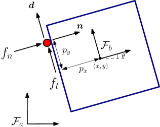
(a) Planar pushing system with world frame $\mathcal{F}_{a}$ and body frame $\mathcal{F}_{b}$. We denote the length of the square as $a$.

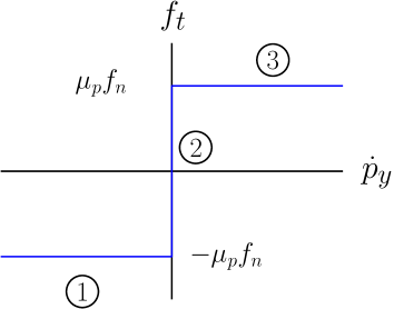
(b) Coulomb’s frictional law. Three contact modes are defined with $\mu_{p}$ the coefficient of friction between the pusher and the object. 1. Sliding right: Friction acts as a force constraint, 2. Sticking: Friction acts as a kinematic constraint, 3. Sliding left: Friction acts as a force constraint.

Figure 1: Problem description for the analytical pushing model. A key difficulty with the analytical model is that it exhibits different hybrid dynamics regimes due to the nature of Coulomb’s friction. This complicates the feedback controller design.

When the pusher interacts with the object, it impresses a normal force $f_{n}$, a tangential frictional force $f_{t}$, and torque $\tau$ about the center of mass. Assuming quasi-static interactions, the applied force causes the object to move in the perpendicular direction to the limit surface, $H(\mbf{w})$, as defined by Zhou et al. [9]. As a result the object twist in the body frame is given by $\mbf{t}={\bm{\nabla}}H(\mbf{w})$ where the applied wrench $\mbf{w}=[f_{n}\,\,f_{t}\,\,\tau]$ can be written as $\mbf{w}=\mbf{J}^{\mathsf{T}}\left(\mbf{n}f_{n}+\mbf{d}{f}_{t}\right)$ with $\mbf{n}=[1\,\,0]^{\mathsf{T}}$, $\mbf{d}=[0\,\,1]^{\mathsf{T}}$, and $\mbf{J}=\left[\begin{array}[]{ccc}1&0&-p_{y}\\ 0&1&p_{x}\end{array}\right]$. The system’s motion equations are

$$\dot{\mbf{x}}=\mbf{f}_{m}(\mbf{x},\mbf{u}_{m})=\left[\begin{array}[]{cc}\mbf{R}\,\mbf{t}\\ \dot{p}_{y}\end{array}\right],\hskip 8.53581pt\mbf{R}=\left[\begin{array}[]{ccc}\cos\theta&-\sin\theta&0\\ \sin\theta&\cos\theta&0\\ 0&0&1\end{array}\right],$$ (1)

where $\mbf{x}=[x\,\,y\,\,\theta\,\,p_{y}]^{\mathsf{T}}$ is the state vector and $\mbf{u}_{m}=[f_{n}\,\,f_{t}\,\,\dot{p}_{y}]^{\mathsf{T}}$ the control input. Due to the nature of physical interactions, the applied forces $f_{n}$, $f_{t}$ and the relative contact velocity $\dot{p}_{y}$ must obey frictional contact laws. Coulomb’s frictional model is depicted in Fig. 1(b), where three different regimes between the pusher and the object are identified: sliding right, sticking, and sliding left. The Coulomb’s frictional model can be expressed using the mathematical constraints $\dot{p}_{y}=0$ and $\left|f_{t}\right|<\mu_{p}\left|f_{n}\right|$ when the pusher is sticking relative to the object, $\dot{p}_{y}>0$ and $f_{t}=\mu_{p}f_{n}$ when the pusher is sliding left relative to the object, and $\dot{p}_{y}<0$ and $f_{t}=-\mu_{p}f_{n}$ when the pusher is sliding right relative to the object. As investigated in Hogan and Rodriguez [1], these discontinuous constraints in the dynamics lead to a hybrid system that makes controller design challenging.

3.2 Data Driven Model

As an alternative to the analytical model, we consider the data-driven approach proposed by Bauza and Rodriguez [18] that better captures the complex frictional interactions between pusher, object, and support surface. Bauza and Rodriguez [18] showed that as few as $100$ samples are enough to train a Gaussian process (GP) to surpass the accuracy of the analytical model.

We train a GP to model for each output using a zero mean prior and the Automatic Relevance Determination (ARD) squared exponential kernel function ${k}(\mbf{x},\mbf{x}^{\prime})={\sigma}_{f}^{2}\text{exp}(-(\mbf{x}-\mbf{x}^{\prime})^{T}{\bm{\Lambda}}^{-1}(\mbf{x}-\mbf{x}^{\prime}))$ where $\sigma_{f}^{2}$ is the signal variance and ${\bm{\Lambda}}$ is a diagonal matrix with the estimated characteristics lengths of each input dimension [19].

To collect data, the robot executes pushes with random initial contact position $p_{y}$ and direction $\beta$ as in Yu et al. [20]. The angle $\beta$ describes the orientation of the pusher relative to the object body frame where $\tan{\beta}=\frac{v_{n}}{v_{t}}$, and $v_{n}$, $v_{t}$ denote the pusher velocity in the body frame. The learning problem is defined as:

Inputs: $[p_{y}\,\,\beta]^{\mathsf{T}}$, as defined above.

Outputs: $\Delta\mbf{x}_{b}=[\Delta x_{b}\,\,\Delta y_{b}\,\,\Delta\theta_{b}]^{\mathsf{T}}$, where $\Delta x_{b}$, $\Delta y_{b}$, and $\Delta\theta_{b}$ represent the displacement of the object’s center and change in orientation in the body frame for the duration of the push $\Delta t$. Figure 2 shows the model obtained for $\Delta\theta_{b}$ depending on the training datapoints.

By leveraging the quasi-static assumption, which neglects inertial effects, the model is learned for a predetermined velocity $V_{nom}$ and scaled proportionally with the velocity of the pusher to recover the object velocity in the body frame as $\dot{\mbf{x}}_{b}=\frac{\left\|\mbf{v}_{p}\right\|}{V_{nom}\Delta t}\Delta\mbf{x}_{b}$, where $\mbf{v}_{p}=[v_{n}\,\,v_{t}]^{\mathsf{T}}$ is the pusher velocity in the body frame.

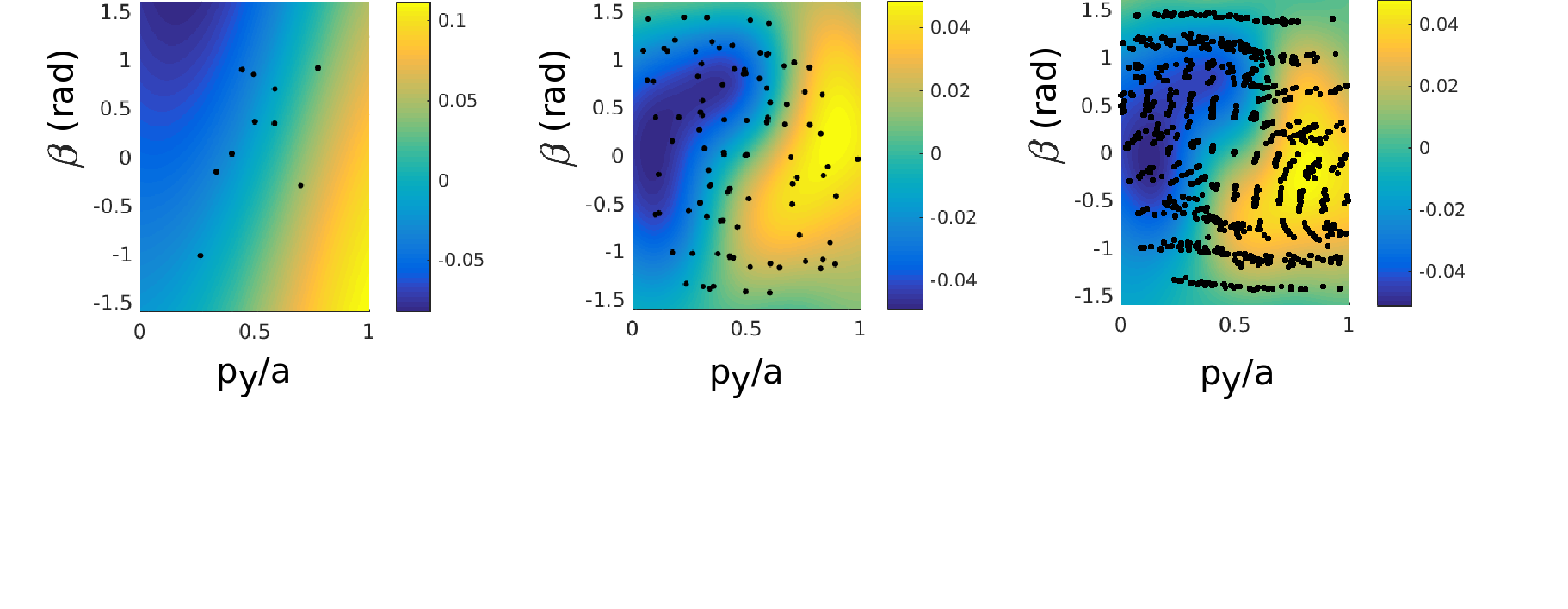
Figure 2: Training data (dots) and learned model for the object’s change in orientation, $\Delta\theta_{b}$ (rad). From left to right the number of datapoints is 10, 100 and 1000. We observe that the model complexity and accuracy increases with the number of training data.

We write the data-driven motion equations in a similar form to (1). The velocity of the pusher relative to the object is resolved in the body frame as

$$\left[\begin{array}[]{cc}\dot{p}_{x}\\ \dot{p}_{y}\end{array}\right]=\mbf{v}_{p}-\mbf{J}\dot{\mbf{x}}_{b}.$$ (2)

The data-driven motion equations are

$$\dot{\mbf{x}}=\mbf{f}_{d}(\mbf{x},\mbf{u}_{d})=\left[\begin{array}[]{cc}\mbf{R}\dot{\mbf{x}}_{b}\\ \dot{p}_{y}\end{array}\right],$$ (3)

where the control input for the data-driven model is $\mbf{u}_{d}=\mbf{v}_{p}$.

4 Controller Design

This section presents the feedback policy design used for real-time control of planar pushing. We control both the analytical and the learned models with a model predictive control (MPC) framework due to its flexibility to the algebraic form of the model, and the possibility to enforce state and action constrains. The model predictive controller acts by simulating the model forward and finding an open loop sequence of control inputs that brings the system close to a desired trajectory. By resolving this optimization in real-time and applying the first action determined in the control sequence, this strategy can act as an effective closed-loop stabilizing policy.

Model Predictive Control (MPC): Given the current error state ${\bar{\mbf{x}}}_{0}$ and a nominal trajectory ($\mbf{x}_{i}^{\star}$, $\mbf{u}_{i}^{\star}$), solve

$$\underset{{\bar{\mbf{x}}}_{i},\hskip 2.84526pt{\bar{\mbf{u}}}_{i}}{\text{min}} {\bar{\mbf{x}}}_{N}^{\mathsf{T}}\mbf{Q}_{N}{\bar{\mbf{x}}}_{N}+\sum_{i=0}^{N-1}\left({\bar{\mbf{x}}}_{i+1}^{\mathsf{T}}\mbf{Q}{\bar{\mbf{x}}}_{i+1}+{\bar{\mbf{u}}}_{i}^{\mathsf{T}}\mbf{R}{\bar{\mbf{u}}}_{i}\right)$$ (4)

subject to $${{\bar{\mbf{x}}}}_{i+1}={{\bar{\mbf{x}}}}_{i}+h\left[\mbf{A}_{i}{{\bar{\mbf{x}}}}_{i}+\mbf{B}_{i}{{\bar{\mbf{u}}}}_{i}\right]\,\hskip 14.22636pt\text{(Linearized Motion Equations)},$$

$$\mbf{x}_{i}\in\,\text{{$\mathcal{X}$} \,\,(State Constraints)},$$

$$\mbf{u}_{i}\in\text{{$\mathcal{U}$} \,\,(Input Constraints)},$$

with integration time step $h$, ${\bar{\mbf{x}}}_{i}=\mbf{x}_{i}-\mbf{x}_{i}^{\star}$ and ${\bar{\mbf{u}}}_{i}=\mbf{u}_{i}-\mbf{u}_{i}^{\star}$. The terms $\mbf{Q}$, $\mbf{Q}_{N}$, and $\mbf{R}$ denote weight matrices associated with the error state, the final error state, and the control input. The optimization is performed by linearizing the dynamics of the system about a desired nominal trajectory with $\mbf{A}_{i}=\frac{\partial\dot{\mbf{x}}}{\partial\mbf{x}}|_{\mbf{x}_{i}^{\star},\mbf{u}_{i}^{\star}}$ and $\mbf{B}_{i}=\frac{\partial\dot{\mbf{x}}}{\partial\mbf{u}}|_{\mbf{x}_{i}^{\star},\mbf{u}_{i}^{\star}}$. The nominal trajectory is computed using the analytical model with sticking interactions to avoid hybridness as done in Zhou and Mason [21].

The model predictive approach offers the flexibility to test the same controller design on both the analytical and the data-driven model. The controller design formulation for both settings is described below.

4.1 Analytical Model

The analytical model uses the control input $\mbf{u}_{m}=[f_{n}\,\,f_{t}\,\,\dot{p}_{y}]$ along with the motion equations (1). We include a constraint on $\left|p_{y}\right|$ to keep the pusher within the object’s edge.

Due to the nature of frictional contacts, as described earlier in Section 3.1, the input constraints are hybrid and not amenable to conventional MPC designed for continuous systems. In this paper, we follow the Family of Modes (FOM) heuristic, as introduced in Hogan and Rodriguez [1], to address this problem.

4.2 Data Driven Model

The data-driven model is more amenable than the analytical model for MPC as it presents continuous differential equations. As such, no particular care needs to be taken with regard to system hybridness and selecting mode sequences. The control input is given directly by the velocity of the pusher in the body frame of the object $\mbf{u}_{d}=\mbf{v}_{p}$ along with the motion equations (3) linearized about the nominal trajectory.

To address the stochastic nature of GPs, we make use of the certainty equivalent approximation [22], which acts by settings random values with their expected value during the optimization process. In the case of the pusher-slider system modeled with GPs, this implies that the mean of the dynamics are propagated forward by setting the state noise value to $0$. This approximation is computationally beneficial since it converts a stochastic optimization problem into a deterministic one. This approximation has been shown to produce good results for linear systems, where the certainty principle is optimal for systems with additive Gaussian noise.

5 Results

This section evaluates the performance of the analytical and data-driven controllers based on their ability to follow a given track. The purpose of the task is to accurately control the motion the object using a point robotic pusher about a desired timed trajectory.

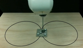
(a) 8-track. Two identical circles of radius $150$mm that intersect. This trajectory is tested at target velocities of $20$mm/s and $80$mm/s.

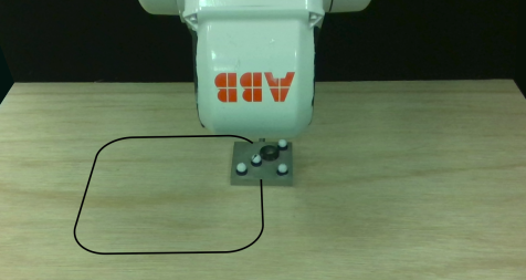
(b) Square track. Four straight lines where the borders between adjacent lines are connected with quarter circles of $80$mm radius. This trajectory is performed at a test velocity of $50$mm/s.

Figure 3: Experimental setup. A metallic rod is attached to an ABB IRB 120 industrial robotic arm to push an object. The pose of the slider is tracked using a Vicon camera system.

5.1 Experimental Setup

Figure 3 depicts the robotic setup and the two target trajectories investigated during the experiments. We use an industrial robotic manipulator (ABB IRB 120) along with a Vicon camera system to track the position of the object as in [23]. The material used for the support surface is plywood with an estimated frictional coefficient of $\mu_{g}=0.35$. The estimated coefficient of friction of the pusher-object interactions is $\mu_{p}=0.3$ and the object is a square of length $90$mm and $0.827$ kg of mass.

The parameters of each controller are tuned to obtain their best performance on the 8-track trajectory at $80$ mm/s. For the data-driven controller, the parameters are only optimized for the model with 5000 data points. The MPC parameters for the analytical model are $\mbf{Q}=[6000,3000,10,0]$, $\mbf{Q}_{N}=\mbf{Q}$, associated with the state $\mbf{x}=[x\,\,y\,\,\theta\,\,p_{y}]^{\mathsf{T}}$ and $\mbf{R}=[0.1,0.001,0.001]$ associated with $\mbf{u}_{m}=[f_{n}\,\,f_{t}\,\,\dot{p}_{y}]^{\mathsf{T}}$. For the learned model, we use $\mbf{Q}=[6000,3000,10,3000]$, $\mbf{Q}_{N}=\mbf{Q}$, and $\mbf{R}=[10,0.001]$, associated with $\mbf{x}=[x\,\,y\,\,\theta\,\,p_{y}]^{\mathsf{T}}$ and $\mbf{u}_{d}=\mbf{v}_{p}$, respectively. Both controllers consider time increments of $h=0.01$s and $N=35$ time steps.

5.2 Model comparison

Table 1 compares the performance of the analytical and the data-driven controller designs on a series of trajectory tracking problems. The performance of each controller is measured by computing the average mean squared error over the duration of the experiment between the desired trajectory and the actual motion of the object’s geometric center (see Fig.4). In this section, we conduct four benchmark experiments for each controller: 1. low tracking velocity ($20$ mm/s) without external perturbations, 2. high tracking velocity ($80$mm/s) without external perturbations, 3. high tracking velocity ($80$mm/s) with external perturbations, and 4. square tracking at $50$mm/s. Two perturbations types are considered in order to test the robustness of the controllers: tangential and normal. Tangential perturbations are applied laterally to the motion of the object by perturbing the initial position of the contact point from its desired position. Normal disturbances are applied orthogonal to the object’s motion by detaching the object away from the robotic pusher by $30$mm.

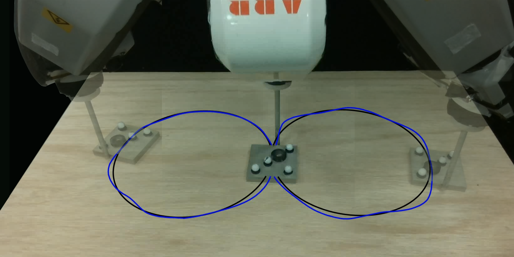
(a) 8-track.

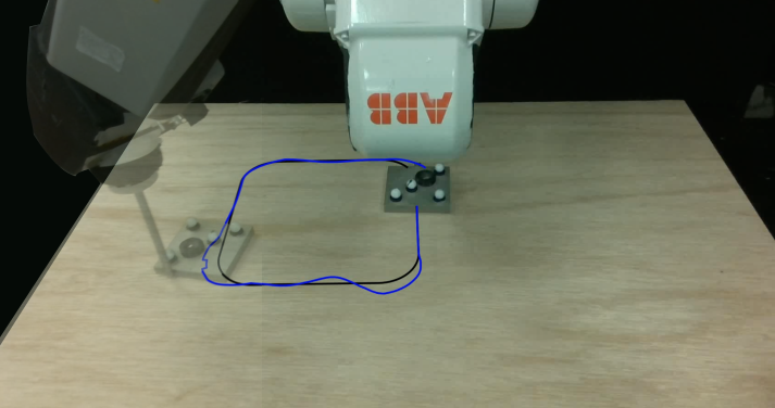
(b) Square track.

Figure 4: Desired trajectory (black) compared with the motion followed by the object’s geometric center (blue) using the analytical controller at 80 and 50 mm/s respectively. The average error for the 8-track example is 9.00mm and 6.05mm for the square.

Table 1: Controller performance comparison

Trajectory	Error (Analytical)	Error (Data-Driven)
8-track no perturbation, v$=80$mm/s	$9.56$ mm	$8.50$ mm
8-track no perturbation, v$=20$mm/s	$2.89$ mm	$6.53$ mm
8-track normal perturbation, v$=80$mm/s	$11.10$ mm	$8.52$ mm
8-track tangential perturbation, v$=80$m/s	$12.37$ mm	$9.28$ mm
Square trajectory, v$=50$mm/s	$4.95$ mm	$6.60$ mm

Table 1 summarizes the tracking performance results for the analytical and data-driven (5000 datapoints) controllers. Both controller designs successfully achieve closed-loop tracking within $10$mm accuracy when no external perturbations are applied. It is worth noting that although the data-driven model only performs marginally better than its model-based counterpart, its controller design is much simpler to implement as it relies on a continuous dynamical model and doesn’t suffer from discontinuous dynamics.

5.3 Influence of data

To evaluate the amount of data required to perform the trajectory tracking task, we run the controller for the data-driven model with an increasing quantity of training data: $N=\{10,20,50,100,200,500,1000,2000,5000\}$. We consider the case of high velocity ($80$mm/s) as it is the most challenging for the controller design. Figure 5 shows that around two hundred points are sufficient to get an accuracy equivalent to that of the analytical model.

When decreasing the amount of data, the control parameters are tuned for the model with $5000$ data points and kept equal across models. The data for the reduced datasets takes subsets such that smaller datasets are always contained within bigger ones.

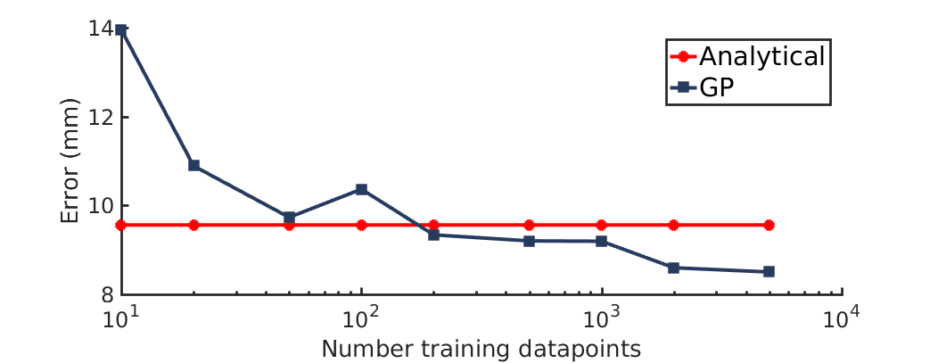
Figure 5: Average error on the 8-track at $80$mm/s depending on the model and the number of training points.

Figure 5 reports the effect of increasing the size of the data to train the GP model. Results show that the tracking performance increases as the model accuracy improves. Perhaps most surprising is that closed-loop performance was possible for the data-driven model with as few as $10$ data points with an accuracy of $14$ mm. This illustrates that feedback control can work with very simple dynamical models that capture the essential behavior of the dynamics. By continuously reassessing the state of the object and recomputing the control action in real-time, the controller can act as to correct previous mistakes and track the desired trajectory.

For GP models trained on random datasets with less than $10$ points, the controller was unstable, i.e., unable to complete the entire lap while remained in contact with the pusher. The data generated for training the GP model in Fig. 5 is at random within the available dataset of experimental pushes. However, interestingly, as later discussed in Section 6, when we carefully select the data used for training the GP, the controller can work with as few as $5$ training points. This result on the lower limit for closed-loop stable tracking was unexpected and shows that data-efficiency can be achieved through a model-based control approach, where the model is directly learned from data.

6 Discussion

This paper explores a data-driven approach to control planar pushing tasks. Results show that learning the dynamics of the system from data and controlling the resulting model can be a data-efficient approach, and can achieve reactive and accurate robot/object interactions. We choose an algebraic form for the model that is continuously differentiable (GP), which is more amenable to apply tools from control theory. The hyperparametrization of the GP model as a function of the data ensures that even if the task has hybrid dynamics, the hybridness is only explicit in the data distribution but not in the algebraic form. In practice, we have found that a minimal amount of data can lead to a stable controller, implying that approximate models of contact interactions can be effective when combined with feedback. Given a set of fixed control parameters, the presented data-driven controller design was able to track both the 8-track and square trajectories show in Fig. 3 at varying speeds, and for different amounts of data and perturbations for the case of the 8-track. This ability to generalize to new tasks is an advantage of model-based control formulations where the model learned can be adapted to new scenarios by leveraging physics.

In this paper, we aimed to answer questions regarding the learning and control representations that are more appropriate for reactive manipulation tasks. What is the level of complexity that should be captured by the motion model? How much data is required? Should system hybridness be explicitly included in the motion model? Our key findings are:

1. Learning a model for control is easier than learning a model for accurate simulation. We are able to get high performance control using a model trained on as little as $5$ hand-selected datapoints or $10$ datapoints selected at random. This result indicates what it is not surprise to the control community, that approximate simple models can enable powerful control mechanisms. We have shown that this simple models can be learned from data.

2. The combination of GP model learning and model predictive control yields a practical and data-efficient framework to learn and control motion models. By stabilizing the motion of an object about a predetermined trajectory, MPC only requires the learned model to be accurate to first order by exploiting feedback.

3. By formulating the model in velocity space, the hybridness inherent of frictional contacts (see Fig.1(b)) softens as the implicit dependence on reaction forces is hidden. This smoothing of the dynamics offers major controller design advantages without compromising the accuracy of the resulting controllers.

A limitation of the proposed methodology is that it relies on tracking a nominal trajectory both in state and actuation spaces. These are required when linearizing the system’s dynamics and are obtained in this paper by relying on planning with respect to the analytical model. Another limitation is that the contact state between the object and the robot is always assumed to be in a contact phase. As such, the controller cannot reason about separation and does not have the ability to switch sides to have better controllability on the object. These generalization would yield a combinatorial input space which would be difficult to handle by a regular GP.

To further improve the performance of the system, we believe that online adaptation of the nominal trajectory (feedforward control) by performing iterative learning control [24] can achieve more aggressive and accurate pushing actions. Most importantly, we are interested in applying the learning control methodology presented in this paper to manipulation problems of higher complexity, with more contact formations and higher degrees of freedom.

References

- Hogan and Rodriguez [2016] F. Hogan and A. Rodriguez. Feedback Control of the Pusher-Slider System: A Story of Hybrid and Underactuated Contact Dynamics. In WAFR, 2016.
- Mason [1986] M. T. Mason. Mechanics and Planning of Manipulator Pushing Operations. IJRR, 5(3), 1986.
- Goyal et al. [1991] S. Goyal, A. Ruina, and J. Papadopoulos. Planar Sliding with Dry Friction Part 1 . Limit Surface and Moment Function. Wear, 143, 1991.
- Lynch et al. [1992] K. M. Lynch, H. Maekawa, and K. Tanie. Manipulation and active sensing by pushing using tactile feedback. In IROS, 1992.
- Salganicoff et al. [1993] M. Salganicoff, G. Metta, A. Oddera, and G. Sandini. A vision-based learning method for pushing manipulation. Technical report, IRCS-93-47, U. of Pennsylvania, Department of Computer and Information Science, 1993.
- Walker and Salisbury [2008] S. Walker and J. K. Salisbury. Pushing Using Learned Manipulation Maps. In ICRA, 2008.
- Lau et al. [2011] M. Lau, J. Mitani, and T. Igarashi. Automatic Learning of Pushing Strategy for Delivery of Irregular-Shaped Objects. In ICRA, 2011.
- Meric et al. [2015] T. Meric, M. Veloso, and H. Akin. Push-manipulation of complex passive mobile objects using experimentally acquired motion models. Autonomous Robots, 38(3), 2015.
- Zhou et al. [2016] J. Zhou, R. Paolini, J. A. Bagnell, and M. T. Mason. A Convex Polynomial Force-Motion Model for Planar Sliding: Identification and Application. In ICRA, 2016.
- Chavan-Dafle and Rodriguez [2017] N. Chavan-Dafle and A. Rodriguez. Sampling-based planning for in-hand manipulations with external pushes. International Symposium on Robotics Research (ISRR). Under Review., 2017.
- Zhou et al. [2017] J. Zhou, R. Paolini, A. M. Johnson, J. A. Bagnell, and M. T. Mason. A probabilistic planning framework for planar grasping under uncertainty. IEEE Robotics and Automation Letters, 2(4):2111–2118, Oct 2017. doi:10.1109/LRA.2017.2720845.
- Arruda et al. [2017] E. Arruda, M. J. Mathew, M. Kopicki, M. Mistry, M. Azad, and J. L. Wyatt. Uncertainty averse pushing with model predictive path integral control. In 2017 IEEE-RAS 17th International Conference on Humanoid Robotics (Humanoids), pages 497–502, Nov 2017. doi:10.1109/HUMANOIDS.2017.8246918.
- Pinto and Gupta [2017] L. Pinto and A. Gupta. Learning to push by grasping: Using multiple tasks for effective learning. In 2017 IEEE International Conference on Robotics and Automation (ICRA), pages 2161–2168, May 2017. doi:10.1109/ICRA.2017.7989249.
- Zeng et al. [2018] A. Zeng, S. Song, S. Welker, J. Lee, A. Rodriguez, and T. A. Funkhouser. Learning synergies between pushing and grasping with self-supervised deep reinforcement learning. CoRR, abs/1803.09956, 2018.
- Finn et al. [2016] C. Finn, I. Goodfellow, and S. Levine. Unsupervised learning for physical interaction through video prediction. In Proceedings of the 30th International Conference on Neural Information Processing Systems, NIPS’16, pages 64–72, USA, 2016. Curran Associates Inc. ISBN 978-1-5108-3881-9. URL http://dl.acm.org/citation.cfm?id=3157096.3157104.
- Ebert et al. [2017] F. Ebert, C. Finn, A. X. Lee, and S. Levine. Self-supervised visual planning with temporal skip connections. arXiv preprint arXiv:1710.05268, 2017.
- Agrawal et al. [2016] P. Agrawal, A. V. Nair, P. Abbeel, J. Malik, and S. Levine. Learning to poke by poking: Experiential learning of intuitive physics. In Advances in Neural Information Processing Systems, pages 5074–5082, 2016.
- Bauza and Rodriguez [2017] M. Bauza and A. Rodriguez. A probabilistic data-driven model for planar pushing. In Robotics and Automation (ICRA), 2017 IEEE International Conference on, pages 3008–3015. IEEE, 2017.
- Rasmussen and Williams [2006] C. Rasmussen and C. Williams. Gaussian Processes for Machine Learning. MIT Press, 2006.
- Yu et al. [2016] K.-T. Yu, M. Bauza, N. Fazeli, and A. Rodriguez. More than a Million Ways to be Pushed. A High-Fidelity Experimental Data Set of Planar Pushing. In IROS, 2016.
- Zhou and Mason [2017] J. Zhou and M. T. Mason. Pushing revisited: Differential flatness, trajectory planning and stabilization. In Proceedings of the International Symposium on Robotics Research (ISRR), 2017.
- Bertsekas [1995] e. a. Bertsekas, Dimitri P. Dynamic Programming and Optimal Control. Athena scientific, 1995.
- Hogan et al. [2018] F. R. Hogan, E. R. Grau, and A. Rodriguez. Reactive Planar Manipulation with Convex Hybrid MPC. In ICRA, 2018.
- Bristow et al. [2006] D. A. Bristow, M. Tharayil, and A. G. Alleyne. A survey of iterative learning control. IEEE Control Systems, 26(3):96–114, 2006.