We review how the AdS/CFT correspondence is motivated within string theory, and discuss how it is generalized to gauge/gravity duality. In particular, we highlight the relation to quantum information theory by pointing out that the Fisher information metric of a Gaussian probability distribution corresponds to an Anti-de Sitter space. As an application example of gauge/gravity duality, we present a holographic Kondo model. The Kondo model in condensed matter physics describes a spin impurity interacting with a free electron gas: At low energies, the impurity is screened and there is a logarithmic rise of the resistivity. In quantum field theory, this amounts to a negative beta function for the impurity coupling and the theory flows to a non-trivial IR fixed point. For constructing a gravity dual, we consider a large $N$ version of this model in which the ambient electrons are strongly coupled even before the interaction with the impurity is switched on. We present the brane construction which motivates a gravity dual Kondo model and use this model to calculate the impurity entanglement entropy and the resistivity, which has a power-law behaviour. We also study quantum quenches, and discuss the relation to the Sachdev-Ye-Kitaev model.

Lectures given at the Theoretical Advanced Study Institute (TASI) Summer School 2017 "Physics at the Fundamental Frontier", 4 June - 1 July 2017, Boulder, Colorado.

1 Introduction

Gauge/gravity duality is one of the major developments in theoretical physics over the last two decades. Based on string theory, it provides a new relation between a quantum field theory without gravity and a gravity theory itself. At a fundamental level within theoretical physics, this has provided new insight into the nature of quantum gravity. Moreover, since in a certain limit gauge/gravity duality maps strongly coupled quantum field theories to classical gravity theories, it has provided a new way for calculating observables in these strongly coupled theories which are generically hard to solve. Gauge/gravity thus provides new unexpected links between previously unrelated areas of physics.

What is a duality? Imagine that a physical system is described by two different actions or Hamiltonians that may involve different encodings of the degrees of freedom. Then, these two different theories are said to be related by a duality. This is visualized in figure 1.

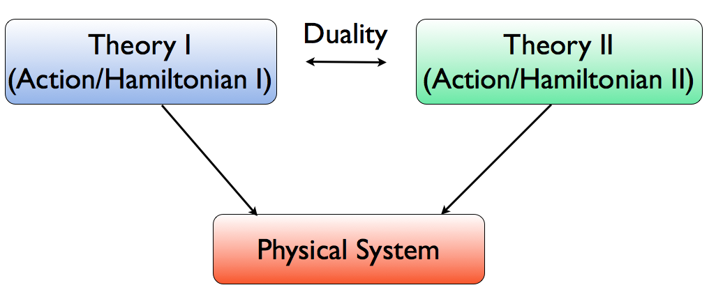
Figure 1: Two physical theories describing the same physical system are related by a duality.

There are many well-known examples for dualities in physics. One of these is the duality between the massive Thirring model and the sine-Gordon model within two-dimensional quantum field theory [1]. This is a boson-fermion duality within quantum field theory. A further example is Montonen-Olive duality of electric and magnetic charges [2], which is an example of a duality between a weakly and a strongly coupled gauge theory or S-duality. This plays also an important role in string theory, together with T-duality [3].

Gauge/gravity duality, as first realized by the AdS/CFT correspondence of Maldacena [4], is a very special duality in the sense that it relates a gravity theory to a gauge theory, i.e. a quantum field theory without gravity. This new relation implies new questions about the nature of gravity itself: How is gravity related to quantum physics? It is equivalent to a non-gravity theory at least in this special context - does this imply that it is non-fundamental? This is an open question which we will not explore in detail here. Nevertheless we note that gauge/gravity duality opens up new issues about the nature of gravity. It is important to emphasize in this context that so far the best understood examples of gauge/gravity duality involve gravity theories with negative cosmological constant, different from the theory describing our Universe in which the cosmological constant is extremely small but positive.

A further important aspect is that generically, gauge/gravity duality relates a quantum gauge theory in flat space to a string theory in curved space. Only in a very particular limit, which we will discuss in detail, this string theory reduces to a classical gravity theory of pointlike particles. On the field theory side, this same limit implies that the quantum gauge theory becomes strongly coupled and the rank of its gauge group goes to infinity.

Applications of gauge/gravity duality. The fact that gauge/gravity duality relates strongly coupled quantum field theories to weakly coupled classical gravity theories provides a new approach to calculating observables in these strongly coupled quantum field theories. Generically, such theories are hard to study since there is no universal approach for calculating observables in them. This is crucially different from weakly coupled quantum field theories, for which perturbation theory is the method of choice and provides very accurate results. An example for an approach to strongly coupled gauge theories is lattice gauge theory, in which space-time is discretized and advanced numerical methods are used. Lattice gauge theory is very successful in calculating observables such as bound state masses, however it is afflicted by the sign problem which renders the description of transport properties very complicated, in particular at finite temperature and density. It is thus desirable to have an alternative approach at hand which allows for comparison. Gauge/gravity duality provides such an approach.

Strongly coupled quantum field theories appear in all areas of physics, including condensed matter physics. Weakly coupled theories may successfully be described in a quasiparticle approach. Quasiparticles are quantum excitationd in one-to-one correspondence with the states in the corresponding free (non-interacting) theory. In strongly-coupled systems however, this map is no longer present. In general, the excitations in these systems are collective modes of the individual degrees of freedom. Gauge/gravity duality provides an elegant way of describing these modes by mapping them to quasinormal modes of the gravity theory. These modes are complex eigenfrequencies of the fluctuations about the gravity background: Their real part is related to the mass of the fluctuations and their complex part to the decay width.

Before we proceed, it is important to stress that to the present day, gauge/gravity duality is a conjecture which has not been proved. The proof is hard in particular since it would require a non-perturbative understanding of string theory in a curved space background, which is not available so far.

These lecture notes only give an outline of the most important concepts. Detailed information on gauge/gravity duality, the AdS/CFT correspondence and its applications may be found for instance in the books [5, 6, 7, 8, 9]. There are also very useful lecture notes of previous TASI schools, see for instance [10, 11]. Further lecture notes on AdS/CFT include [12, 13, 14].

In the present notes, we also include comments on recent developments relating the AdS/CFT correspondence to concepts from quantum information. In the second part of these lectures, we focus on the Kondo model and a variant of it with a gravity dual. This provides a new example for constructing a gravity dual, and its applications. This provides a further entry in the list of examples of gauge/gravity duality. Related further lectures at TASI 2017 are those by Harlow [15] and DeWolfe [16] in particular.

2 AdS/CFT correspondence

2.1 Statement of the correspondence

Let us begin by considering the best understood example of gauge/gravity duality, the AdS/CFT correspondence. Here, ‘AdS’ stands for ‘Anti-de Sitter space’ and and ‘CFT’ for ‘conformal field theory. The Dutch physicist Willem de Sitter was a friend of Einstein. The prefix ‘Anti’ refers to the fact that a crucial sign changes from plus to minus. In fact, Anti-de Sitter space is a hyperbolic space with a negative cosmological constant.

In this example a four-dimensional CFT, ${\cal N}=4$ $SU(N)$ Super Yang-Mills theory, is conjectured to be dual to gravity in the space AdS${}_{5}\times$ S⁵. This was proposed along with other examples for AdS/CFT by Maldacena in his seminal paper [4] in 1997. As we will see, the two theories have the same amount of degrees of freedom per unit volume and the same global symmetries. We will first state the duality and then explain it in detail. The AdS/CFT correspondence states that

$\mathcal{N}=4$ Super Yang-Mills (SYM) theory with gauge group $SU(N)$ and Yang-Mills coupling $g_{\mathrm{YM}}$

is dynamically equivalent to
Type IIB superstring theory on AdS${}_{5}\times S^{5}$, with string length $l_{s}=\sqrt{\alpha^{\prime}}$ and coupling constant $g_{s}$. The radius of curvature of both AdS₅ and $S^{5}$ is $L$, and there are $N$ units of $F_{(5)}$ flux on $S^{5}.$

The two free parameters on the field-theory side, i.e. $g_{\mathrm{YM}}$ and $N$, are related to the free parameters $g_{s}$ and $L/\sqrt{\alpha^{\prime}}$ on the string theory side by

$$g_{\mathrm{YM}}^{2}=2\pi g_{s}\quad\mbox{and}\quad 2g_{\mathrm{YM}}^{2}N=L^{4}/\alpha^{\prime 2}.$$

For understanding this duality and its motivation in detail, let us first recall some properties of the ingredients involved. We begin with the field theory side and introduce conformal field theories and ${\cal N}=4$ supersymmetry.

2.2 Prerequisites for AdS/CFT

2.2.1 Conformal symmetry

An essential aspect for the AdS/CFT correspondence is that the quantum field theory involved is a conformal field theory (CFT). Such a theory consists of fields that transform covariantly under conformal coordinate transformation. These leave angles invariant (locally) and in flat $d$-dimensional spacetime are defined by the following transformation law of the metric,

$$dx^{\prime}_{\mu}dx^{\prime\mu}=\Omega^{-2}(x)dx_{\mu}dx^{\mu}\,.$$ (2.1)

Infinitesimally, with $\Omega(x)=1-\sigma(x)$ and $x^{\prime\mu}=x^{\mu}+v^{\mu}(x)$, this gives rise to the conformal Killing equation

$${\partial}_{\mu}v_{\nu}+{\partial}_{\nu}v_{\mu}=2\sigma(x)\eta_{\mu\nu}\,,\qquad\sigma(x)=\frac{1}{d}{\partial}\cdot v\,.$$ (2.2)

In $d=2$ dimensions, this reduces to the Cauchy-Riemann equations, which are solved by any holomorphic function. This implies that in $d=2$, conformal symmetry is infinite dimensional and thus leads to an infinite number of conserved quantities. In more than two dimensions however, conformal symmetry is finite dimensional and the only solutions to the conformal Killing equation (2.2) are

$$v^{\mu}(x)=a^{\mu}+\omega^{\mu}{}_{\nu}x^{\nu}+\lambda x^{\mu}+b^{\mu}x^{2}-2(b\cdot x)x^{\mu}\,;\quad\omega_{\mu\nu}=-\omega_{\nu\mu}\,,\sigma(x)=\lambda-2b\cdot x\,.$$ (2.3)

In $d>2$, the conformal Killing vector $v_{\mu}(x)$ is at most quadratic in $x$. It contains translations (of zeroth order in $x$), rotations and scale transformations (both linear in $x$) and special conformal transformations (quadratic in $x$). The scalar $\lambda$, the vectors $a_{\mu}$ and $b_{\mu}$ and the antisymmetric matrix $\omega_{\mu\nu}$ contain a total of

$$1+2d+d(d-1)/2=(d+1)(d+2)/2$$ (2.4)

free parameters. In Euclidean signature, the symmetry group generated by these transformations is $SO(d+1,1)$, while in Lorentzian signature, it is $SO(d,2)$. Let us examine the algebra associated to the infinitesimal transformations (2.3) with parameters $(a^{\mu},\omega^{\mu\nu},\lambda,b^{\mu})$ for the Lorentzian case. The generator for translations is the momentum operator $P_{\mu}$. The generator for Lorentz transformations is denoted by $L_{\mu\nu}$. The generator for scale transformations is $D$ and the generator for special conformal transformations is $K_{\mu}$. The conformal algebra consists of the Poincaré algebra supplemented by the relations

$$[L_{\mu\nu},K_{\rho}] =i(\eta_{\mu\rho}K_{\nu}-\eta_{\nu\rho}K_{\mu})\,,\qquad[D,P_{\mu}]=iP_{\mu}\,,$$ (2.5)

$$[D,K_{\mu}] =-iK_{\mu}\,,\qquad[D,L_{\mu\nu}]=0\,,\qquad[K_{\mu},K_{\nu}]=0\,,$$ (2.6)

$$[K_{\mu},P_{\nu}] =-2i(\eta_{\mu\nu}D-L_{\mu\nu})\,.$$ (2.7)

For the representations we postulate

$$[D,\phi(0)]=-i\Delta\phi(0)$$ (2.8)

for any field $\phi(x)$. This implies

$$\phi(x)\rightarrow\phi^{\prime}(x^{\prime})=\lambda^{-\Delta}\phi(x)$$ (2.9)

for $x\rightarrow x^{\prime}=\lambda x$. $\Delta$ is the scaling dimension of the field $\phi$. For an infinitesimal transformation this gives

$$\delta_{D}\phi\equiv[D,\phi(x)]=-i\Delta\phi(x)-ix^{\mu}{\partial}_{\mu}\phi(x)\,,$$ (2.10)

with similar relation for the other conformal transformations $\delta_{P}\phi$, $\delta_{L}\phi$, $\delta_{K}\phi$.

For organising the representations, it is useful to define the quasiprimary fields which satisfy

$$[K_{\mu},\phi(0)]=0\,.$$ (2.11)

This defines the fields of lowest scaling dimension in an irreducible representation of the conformal algebra. All other fields in this multiplet, the conformal descendents of $\phi$, are obtained by acting with $P_{\mu}$ on the quasiprimary fields.

The infinitesimal transformations $\delta\phi$ give rise to the conformal Ward identities

$$\sum\limits_{i=1}^{n}\langle\phi_{1}(x_{1})\dots\delta\phi_{i}(x_{i})\dots\phi_{n}(x_{n})\rangle=0\,.$$ (2.12)

For scalar conformal fields this implies

$$\langle\phi_{1}(x_{1})\phi_{2}(x_{2})\rangle=\begin{cases}\frac{c}{(x_{1}-x_{2})^{2\Delta}}&\text{if}\;\;\Delta_{1}=\Delta_{2}=\Delta\,,\\ 0&\text{otherwise.}\end{cases}$$ (2.13)

For fields with spin, the conformal transformation acts also on the spacetime indices and reads

$$\delta_{v}\mathcal{O}(x)=-{\cal L}_{v}\mathcal{O}(x)\,,\qquad{\cal L}_{v}\equiv v\cdot{\partial}_{x}+\frac{\Delta}{d}{\partial}\cdot v-\frac{i}{2}{\partial}^{[\mu}v^{\nu]}L_{\mu\nu}\,,$$ (2.14)

for an operator $\mathcal{O}(x)$ of arbitrary spin. The Lorentz generator $L_{\mu\nu}$ acts on the spin indices. For these operators, the conformal correlation functions are more involved. However, conformal symmetry still fixes the two- and three point functions up to a small number of independent contributions [17, 18].

2.2.2 ${\cal N}=4$ Supersymmetry

The ${\cal N}=4$ $SU(N)$ Super-Yang-Mills theory has some very special properties which are at the origin of it possessing a gravity dual. First of all, it was shown [19, 20] that this theory is conformally invariant even when quantised; its beta function vanishes to all orders in perturbation theory and also non-perturbative contributions are absent. A further important property is that this theory has a global $SU(4)$ symmetry, which is isomorphic to $SO(6)$. We will see that both the $SO(4,2)$ conformal symmetry as well as $SU(4)$ are also realized as isometries in the dual gravity theory. We also note that ${\cal N}=4$ Super Yang-Mills theory is invariant under S-duality [21].

For the ${\cal N}=4$ theory, the global $SU(4)$ symmetry is realized as an R symmetry of the supersymmetry algebra. This algebra has four supersymmetry generators which satisfy the anticommutation relations

$$\{Q^{a}_{\alpha},\bar{Q}_{b\dot{\beta}}\}=2\sigma^{\mu}{}_{\alpha\dot{\beta}}P_{\mu}\delta^{a}{}_{b}\,,\qquad a=1,2,3,4\,,$$ (2.15)

with $\sigma^{\mu}{}=(\mathbbm{1},\vec{\sigma})$ and $\vec{\sigma}$ the three Pauli matrices. (2.15) is invariant under $SU(4)$ rotations. This algebra may be combined with the conformal algebra into a superconformal algebra. This requires the introduction of further fermionic generators, the special superconformal generators $S^{a}_{\alpha}$ that satisfies

$$\{S^{a}_{\alpha},\bar{S}_{b\dot{\beta}}\}=2\sigma^{\mu}{}_{\alpha\dot{\beta}}K_{\mu}\delta^{a}{}_{b}\,,\qquad a=1,2,3,4,$$ (2.16)

with $K_{\mu}$ the generator of special conformal transformations. We note that the anticommutation relation for the generators $S^{a}_{\alpha}$ (2.16) is formally similar to the one for the generators $Q^{a}_{\alpha}$ given by (2.15), with the momentum operator $P_{\mu}$ replaced by the special conformal transformations $K_{\mu}$. The operators $P_{\mu},L_{\mu\nu},D,K_{\mu}$ together with the $Q^{a}_{\alpha},S^{a}_{\alpha}$ form the superconformal algebra associated to the superconformal group $SU(2,2|4).$

Fields		$SU(4)$ rep.
Gauge field	$A_{\mu}$	$\mathbf{1}$
Complex fermions	$\lambda^{a}_{\alpha}$	$\mathbf{4}$
Real scalars	$X^{i}$	$\mathbf{6}$

Table 1: Supermultiplet of N=4 Supersymmetry.

The elementary fields of ${\cal N}=4$ Super Yang-Mills theory are organized in a single multiplet of $SU(4)$, as shown in table 1. The $SU(N)$ gauge field is a singlet of $SU(4)$. Moreover, the supermultiplet involves four complex Weyl fermions $\lambda^{a}_{\alpha}$ in the fundamental representation ${\bf 4}$ of $SU(4)$ and six real scalars $X^{i}$ in the representation ${\bf 6}$ of $SU(4)$. Note that due to the supersymmetry, both the Weyl fermions and the scalars are in the adjoint representation of the gauge group $SU(N)$ since they are in the same multiplet as the gauge field.

The action of ${\cal N}=4$ Super Yang-Mills theory reads

$$S =\mathrm{tr}\int\!d^{4}x\left(-\frac{1}{2g_{\mathrm{YM}}{}^{2}}F_{\mu\nu}F^{\mu\nu}-i\sum\limits_{a=1}^{4}\bar{\lambda}^{a}\bar{\sigma}^{\mu}D_{\mu}\lambda_{a}-\sum\limits_{i=1}^{6}D_{\mu}\phi^{i}D^{\mu}\phi^{i}\right.$$

$$\;\hskip 14.22636pt\left.+g_{\mathrm{YM}}{}\sum\limits_{a,b,i}C^{ab}{}_{i}\lambda_{a}[\phi^{i},\lambda_{b}]+g_{\mathrm{YM}}{}\sum\limits_{a,b,i}\bar{C}_{iab}\bar{\lambda}^{a}[\phi^{i},\bar{\lambda}^{b}]+\frac{g_{\mathrm{YM}}{}^{2}}{2}\sum\limits_{i,j}[\phi^{i},\phi^{j}]^{2}\right)\,,$$ (2.17)

with $gg_{\mathrm{YM}}$ the Yang-Mills coupling. The $C^{ab}_{i}$ are Clebsch-Gordan coefficients that couple two $\bf 4$ representations to one $\bf 6$ representation of the algebtra of $SU(4)_{R}$. We note that in addition to the kinetic terms, this action contains interactions between three and four gauge fields via the non-abelian gauge-field commutators in $F^{\mu\nu}$, as well as Yukawa interaction terms between two fermions and a scalar, and a quartic scalar interaction.

2.2.3 Large $N$ limit

The large $N$ limit plays an essential role for the AdS/CFT correspondence. It corresponds to a saddle point approximation. As realized by ’t Hooft in 1974 [22], the perturbative expansion of fields in the adjoint representation of the $SU(N)$ gauge group may be reorganized using a double-line notation.

A field $\phi$ in the adjoint representation may be written as

$$\phi=\phi^{A}T^{A}\;\Leftrightarrow\;(\phi)^{i}{}_{j}=\phi^{A}(T^{A})^{i}{}_{j}\,,$$ (2.18)

where the $T^{A}$ are the $N^{2}-1$ generators of $SU(N)$. These are matrices with indices $i,j$. If $\phi$ is a scalar field in 3+1 dimensions, then its propagator in configuration space is given by

$$\langle\phi^{i}{}_{j}(x)\phi^{k}{}_{l}(y)\rangle\,=\,\delta^{i}{}_{l}\delta^{k}{}_{j}\frac{g^{2}}{4\pi^{2}(x-y)^{2}}\,,$$ (2.19)

where $g$ is a typical coupling in the theory. The Kronecker deltas enter from the $SU(N)$ completeness relation

$$\sum\limits_{A=1}^{N^{2}-1}(T^{A})^{i}{}_{j}(T^{A})^{k}{}_{l}=\delta^{i}{}_{l}\delta^{k}{}_{j}-\frac{1}{N}\delta^{i}{}_{j}\delta^{k}{}_{l}\,,$$ (2.20)

in which the second term is suppressed for $N\rightarrow\infty$. For scalar fields, $g$ in (2.19) may be the coupling of a cubic interaction term; a quartic interaction term may then enter with coefficient $g^{2}$. In Yang-Mills theory, $g$ will be the gauge coupling. It will turn out to be extremely useful to define the ’t Hooft coupling

$$\lambda=g^{2}N\,.$$ (2.21)

Let us now count how the contributions corresponding to Feynman diagrams scale with $N$ and with $\lambda$. Note that in the normalization for the propagators chosen in (2.19), the vertices scale as $1/g^{2}$. Also, the sum over traces of indices contributes a factor of $N$ for every closed loop. Assembling all the ingredients, we find that the Feynman diagrams scale as

$$f(\lambda,N)\sim N^{V-E+F}\lambda^{E-V}=N^{\chi}\lambda^{E-V}\,,$$ (2.22)

where $V$, $E$ and $F$ are the numbers of vertices, edges and faces of the surfaces created by the Feynman diagrams, respectively. $\chi$ is the Euler characteristic given by

$$\chi=V-E+F=2-2G\,,$$ (2.23)

with $G$ the genus of the surface. We see that the leading order in $N$ is given by $G=0$, i.e. by the planar diagrams. Two examples for double-line vacuum Feynman diagrams are given in figure 2: The planar diagram scales as $N^{2}$ while the non-planar diagrams is $1/N^{2}$ suppressed and scales as $N^{0}$. We note that the Feynman diagrams shown look like string-theory diagrams with strings splitting and joining. This provides a hint that large $N$ quantum field theories are related to string theories. In the simple example with scalar fields considered here, it is not possible to determine exactly which string theory is given by the collection of large $N$ field-theory Feynman diagrams. The AdS/CFT correspondence however provides a map between well-defined field theories and string theories.

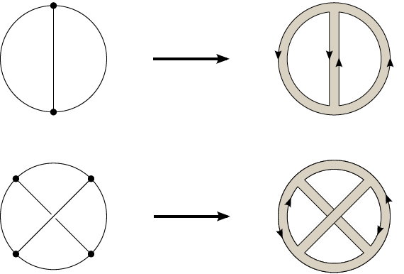
Figure 2: Replacing single-line by double-line Feynman diagrams. Top: Planar diagram of genus zero. Bottom: Non-planar diagram of genus one.

2.2.4 AdS spaces

Anti-de Sitter (AdS) spaces play an important role in the AdS/CFT correspondence. This has several reasons: First of all, the isometries of AdS space in $d+1$ dimensions form the group $SO(d,2)$, which corresponds to the conformal group of a CFT in $d$ dimensions. Moreover, AdS space has a constant negative curvature and a boundary at which we may imagine this CFT to be defined.

The embedding of $(d+1)$-dimensional AdS space into $(d+2)$-dimensional flat Minkowski spacetime is provided by the surface satisfying

$$X_{1}{}^{2}+X_{2}{}^{2}+\dots+X_{d}{}^{2}-X_{0}{}^{2}-X_{d+1}{}^{2}=-L^{2}\,,$$ (2.24)

where $X_{0}$, $X_{1}$, $\dots$ $X_{d+1}$ are the coordinates of $(d+2)$-dimensional Minkowski space. $L$ is referred to as the AdS radius. We note that in Lorentzian signature, the symmetry of the isometries of AdS_d+1 is thus $SO(d,2)$, which coincides with the symmetry of a CFT_d, i.e. a conformal field theory in $d$ dimensions with Lorentzian signature. In Euclidean signature, the sign in front of $X_{0}{}^{2}$ becomes a plus and the symmetry is $SO(d+1,1)$.

The boundary of AdS_d+1 is located at the limit of all coordinates $X_{M}$ becoming asymptotically large. For large $X_{M}$, the hyperboloid given by (2.24) approaches the light-cone in $\mathbbm{R}^{d,2}$, given by

$$-X_{0}{}^{2}+\sum\limits_{i=1}^{d}X_{i}{}^{2}-X_{d+1}{}^{2}=0\,.$$ (2.25)

The boundary corresponds to the set of all lines on the light cone given by (2.25) which originate from the origin of $\mathbbm{R}^{d,2}$, i.e. $0\in\mathbbm{R}^{d,2}$. This space corresponds to a conformal compactification of Minkowski space.

A set of coordinates that solves (2.24) is

$$X^{0} =\ L\,\cosh\rho\,\cos\tau\,,$$ (2.26)

$$X^{d+1} =\ L\,\cosh\rho\,\sin\tau\,,$$

$$X^{i} =\ L\,\Omega_{i}\,\sinh\rho\,,\qquad\mbox{for}\;i=1,\dots,d\,,$$

where $\Omega_{i}$ with $i=1,\ldots,d$ are angular coordinates satisfying $\sum_{i}\Omega_{i}^{2}=1.$The remaining coordinates take the ranges $\rho\in\mathbbm{R}_{+}$ and $\tau\in[0,2\pi[.$ The coordinates $(\rho,\tau,\Omega_{i})$ are referred to as global coordinates of AdS_d+1. It is convenient to introduce a new coordinate $\theta$ by $\tan\theta=\sinh\rho.$ Then the metric associated to the parametrization (2.26) becomes that of the Einstein static universe $\mathbbm{R}\times S^{d}$,

$$ds^{2}=\frac{L^{2}}{\cos^{2}\theta}\;\big{(}-\,d\tau^{2}\ +\ d\theta^{2}\ +\ \sin^{2}\theta\,d\Omega_{d-1}^{2}\big{)}\,.$$ (2.27)

Since $0\leq\theta<\frac{\pi}{2}$, this metric covers half of $\mathbbm{R}\times S^{d}$.

It is often useful to consider a metric in local coordinates on AdS_d+1. This is obtained from the parametrization, with $\vec{x}=(x^{1},\dots,x^{d-1})$,

$$X_{0} =\frac{L^{2}}{2r}\left(1+\frac{r^{2}}{L^{4}}(\vec{x}^{2}-t^{2}+L^{2})\right)\,,$$

$$X_{i} =\frac{rx_{i}}{L}\;\;\mathrm{for}\;\;i\in\{1,\dots,d-1\}\,,$$

$$X_{d} =\frac{L^{2}}{2r}\left(1+\frac{r^{2}}{L^{4}}(\vec{x}^{2}-t^{2}-L^{2})\right)\,,$$

$$X_{d+1} =\frac{rt}{L}\,.$$ (2.28)

This covers only one half of the AdS spacetime since $r>0$. The corresponding metric is referred to as Poincaré metric and reads

$$ds^{2}=\frac{L^{2}}{r^{2}}dr^{2}+\frac{r^{2}}{L^{2}}\eta_{\mu\nu}dx^{\mu}dx^{\mu}\,.$$ (2.29)

The boundary is located at $r\rightarrow\infty$. The embedding of the Poincaré patch into global AdS is shown in figure 3.

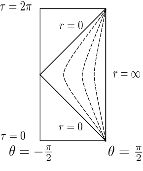
Figure 3: Within AdS₂, the Poincaré coordinates cover the triangular region shown. The dashed lines correspond to fixed constant values of $r$. The boundary is at $r=\infty$. $\theta$ and $\tau$ are as defined in (2.27); for AdS₂, the coordinate $\theta$ ranges from $-\pi/2\leq\theta\leq\pi/2$ since the sphere $S^{0}$ consists of two points.

A further choice of coordinates is obtained by introducing the coordinate $z\equiv L^{2}/r$, for which the Poincaré metric (2.29) becomes

$$ds^{2}=\frac{L^{2}}{z^{2}}\left(dz^{2}+\eta_{\mu\nu}dx^{\mu}dx^{\nu}\right)\,.$$ (2.30)

In this case, the boundary is located at $z\rightarrow 0$. There is a coordinate singularity at the boundary, but the space remains regular there since the curvature remains finite.

Note that the Ricci scalar and cosmological constant for Anti-de Sitter space are both negative,

$$R=-\frac{d(d+1)}{L^{2}}\,,\qquad\Lambda=-\frac{d(d-1)}{2L^{2}}\,.$$ (2.31)

2.3 Fisher information metric

In the preceding section we have collected all the necessary ingredients for formulating the AdS/CFT correspondence. Before now proceding to see how the AdS/CFT conjecture arises within string theory, we take a step back and for further motivation consider the concept of Fisher information. This concept from statistical mechanics gives rise to a metric on the space of probability distributions. This provides a link between geometry and quantum-mechanical probability densities in particular. We will use this to show how a Gaussian probability distribution, which arises naturally for a quantum field theory in the large $N$ limit, leads to an Anti-de Sitter metric [23, 24, 25]. Relating AdS/CFT to concepts from information theory is a new research direction which currently triggers a wealth of developments, as discussed also in further lectures at this TASI 2017 School, see for instance [15].

Consider a normalized probability density with $x$ as stochastic variable and $\vec{\theta}$ a set of external parameters A probability distribution $p(x,\vec{\theta})$ is normalized to one,

$$\int\!dxp(x,\vec{\theta})=1\,,$$ (2.32)

and the expectation value of an operator $\mathcal{O}$ is given by

$$\langle\mathcal{O}\rangle=\int\!dx\,p(x,\vec{\theta})\mathcal{O}(x)\,.$$ (2.33)

We define the spectrum $\gamma(x,\vec{\theta})=-\ln p(x,\vec{\theta})$, which allosw us to write the von Neumann entropy as

$$S(\vec{\theta}) =-\int\!dxp(x,\vec{\theta})\ln p(x,\vec{\theta})$$

$$=\int\!dxp(x,\vec{\theta})\gamma(x,\vec{\theta})=\langle\gamma\rangle\,.$$ (2.34)

The Fisher metric is then defined as

$$g_{\mu\nu}(\vec{\theta})=\int dxp(x,\vec{\theta})\frac{{\partial}\gamma(x,\vec{\theta})}{{\partial}\theta^{\mu}}\frac{{\partial}\gamma(x,\vec{\theta})}{{\partial}\theta^{\nu}}=\langle{\partial}_{\mu}\gamma{\partial}_{\nu}\gamma\rangle\,.$$ (2.35)

Now let us evaluate this general expression for a Gaussian distribution $p_{G}(x,\vec{\theta})$ as relevant for a saddle point approximation arising for instance in the large $N$ limit,

$$p_{G}(x,\vec{\theta})=p(x,\bar{x},\sigma)=\frac{1}{\sqrt{2\pi}\sigma}\exp\left(-\frac{(x-\bar{x})^{2}}{2\sigma^{2}}\right)\,,$$ (2.36)

where $\bar{x}$ is the mean of the distribution and $\sigma$ its standard deviation. For the Gaussian, the Fisher metric (2.35) becomes

$$g_{\mu\nu}d\theta^{\mu}d\theta^{\nu}=\frac{1}{\sigma^{2}}(d\bar{x}^{2}+2\,d\sigma^{2})\,.$$ (2.37)

Subject to a suitable rescaling of the coordinates, this is the metric of Euclidean AdS₂, with the standard deviation $\sigma$ playing the role of the radial coordinate. The higher-dimensional case is obtained from a distribution with several variables $x_{1}$, $\dots$, $x_{d}$, for which

$$p_{G}(x_{1},\dots,x_{d},\bar{x}_{1},\dots,\bar{x}_{d},\sigma)=\frac{1}{\sqrt{2\pi}\sigma^{d}}\exp\left(-\frac{\sum\limits_{i=1}^{d}(x_{i}-\bar{x}_{i})^{2}}{2\sigma^{2}}\right)\,.$$ (2.38)

The Fisher metric for a Gaussian distribution is thus an AdS metric! This is an interesting fact, however, so far we do not know what determines the dynamics of this metric - there is no action on the gravity side. So the relation found is not an example of a gauge/gravity duality.

With this additional motivation, let us now return to our example where the dynamics is determined explicitly on both sides of the duality, i.e. the AdS/CFT correspondence as proposed by Maldacena.

2.4 String theory origin of the AdS/CFT correspondence

Given the motivation presented in the preceding subsection, let us return to the duality example where the dynamics of the gravitational theory is determined, i.e. the duality proposed by Maldacena in 1997 [4]. Let us consider this duality for D3-branes within string theory. In full generality, the conjecture states that ${\cal N}=4$ $SU(N)$ Super-Yang-Mills theory is dual to type IIB string theory on AdS₅ $\times$ $S^{5}$ for all values of $N$ and $\lambda$. While this is a very beautiful idea, performing actual explicit calculations for testing this proposal requires to consider particular low-energy limits which we will discuss in detail. This is due to the fact that quantum string theory on curved backgrounds has not yet been formulated. This is also a reason why it is hard to provide an actual proof for the AdS/CFT proposal.

2.4.1 Motivating AdS/CFT from string theory

As a particular limit, we consider weakly coupled string theory with string coupling $g_{s}\ll 1$, keeping $L/{\sqrt{\alpha^{\prime}}}$ fixed. The leading order is the classical string theory with $g_{s}=0$, which means to only tree-level string diagrams are taken into account. On the CFT side, since $g_{\mathrm{YM}}^{2}=2\pi g_{s}$ this implies $g_{YM}^{2}=\lambda/N\rightarrow 0$. This in turn implies that $N\rightarrow\infty$ since $\lambda=L^{4}/(2\alpha^{\prime 2})$ remains finite. We are thus considering the ’t Hooft limit. The duality conjectured in this limit, where $\lambda$ is fixed but may be small, and the dual field theory contains classical strings, is often referred to as the strong form of the AdS/CFT correspondence. There is also the weak form of AdS/CFT in which additionally, $\lambda$ is taken to be very large such that the CFT involved becomes strongly coupled. In this case, the strongly coupled CFT is mapped to a classical gravity theory of pointlike particles, since $\alpha^{\prime}=\ell_{s}^{2}$ (with $\ell$ the string length) becomes asymptotically small. The gravity theory involved is type IIB supergravity in the example considered. Type IIB supergravity admits D3-brane solutions. The possible limits of the AdS/CFT correspondence are collected together in table 2.

	${\cal N}=4$ SYM theory	IIB theory on $AdS_{5}$ $\times$ $S^{5}$
Strongest form	any $N$ and $\lambda$	Quantum string theory, $g_{s}\neq 0$, $\alpha^{\prime}\neq 0$
Strong form	$N\rightarrow\infty$, $\lambda$ fixed but arbitrary	Classical string theory, $g_{s}\rightarrow 0$, $\alpha^{\prime}\neq 0$
Weak form	$N\rightarrow\infty$, $\lambda$ large	Classical supergravity, $g_{s}\rightarrow 0$, $\alpha^{\prime}\rightarrow 0$

Table 2: Different forms of the AdS/CFT correspondence

Let us now consider D3-branes to motivate the weak form of the AdS/CFT correspondence. These branes may be viewed from two different perspectives: The open and the closed string perspective. It is crucial for the correspondence that in the low-energy limit where only massless degrees of freedom contribute, open strings give rise to gauge theories while closed strings give rise to gravity theories.

Open string perspective. We begin with the open string perspective on D3-branes. For $g_{s}N\ll 1$, D-branes may be visualised as higher-dimensional charged objectd on which open strings may end. The ‘D’ stands for Dirichlet boundary condition. Consider a stack of $N$ D3-branes embedded in 9+1 flat spacetime dimensions. (Recall that in 9+1 dimensions, superstring theory is anomaly free and thus consistent.) Neumann and Dirichlet boundary conditions are imposed on the string modes according to table 3.

	0	1	2	3	4	5	6	7	8	9
$N\,D3$	$\bullet$	$\bullet$	$\bullet$	$\bullet$	-	-	-	-	-	-

Table 3: Embedding of $N$ coincident D3–branes in flat ten-dimensional spacetime.

For $N$ coincident D3-branes, the open strings are described by a Dirac-Born-Infeld (DBI) action with gauge group $U(N)$, with integration over the 3+1-dimensional worldvolume of the branes. In flat ten-dimensional space, the DBI action is given by

$$S_{\mathrm{DBI}}= -T_{3}\,\mathrm{tr}\,\int\!d^{4}xe^{-\varphi}\sqrt{-\mathrm{det}(P[g]+2\pi\alpha^{\prime}F)}\;$$

$$+\,\mathrm{fermionic\;partners}\,,$$ (2.39)

where $T_{3}\equiv 2/((2\pi)^{3}\alpha^{\prime 2}g_{s})$ is the brane tension, $\varphi$ is the dilaton, and $P[g]$ is the pullback of the metric to the worldvolume of the branes. $F$ is the field strength tensor of the gauge field associated to the brane charge. We now consider low-energy excitations with $E\ll\alpha^{\prime}{}^{-1/2}$, such that only massless excitations are taken into account. In this limit, the DBI action reduces to

$$S_{\mathrm{DBI}} =-\frac{1}{2\pi g_{s}}\;\mathrm{tr}\,\int\!d^{4}x\,\left(\frac{1}{2}F_{\mu\nu}F^{\mu\nu}+\sum\limits_{i=1}^{6}{\partial}^{\mu}\phi^{i}{\partial}_{\mu}\phi^{i}-\pi g_{s}\sum\limits_{i,j=1}^{6}[\phi^{i},\phi^{j}]^{2}\right)$$

$$\hskip 14.22636pt\,+\,\mathrm{fermions}\,+\,{\cal O}(\alpha^{\prime})\,,$$ (2.40)

where the six scalars $\phi^{i}=\phi^{iA}T^{A}$ in the adjoint representation of $U(N)$ arise from the pull-back of the metric to the world-volume of the $N$ D3-branes. They are given by $X^{i+3}=2\pi\alpha^{\prime}\phi^{i}$ with the $X^{i+3}$ the coordinates in the directions perpendicular to the brane.

The total action for the D3-branes is

$$S_{D3}=S_{\mathrm{DBI}}+S_{\mathrm{closed}}+S_{\mathrm{int}}\,,$$ (2.41)

where $S_{\mathrm{closed}}$ describes the closed string excitations in the ten-dimensional space and $S_{\mathrm{int}}$ the interaction between open and closed string modes. In the low-energy limit $\alpha^{\prime}\rightarrow 0$, the open strings decouple from any closed string excitations in the 9+1-dimensional space: In (2.41), $S_{\mathrm{closed}}$ becomes a free theory of massless metric fluctuations, and $S_{\mathrm{int}}$ goes to zero. In this limit we are thus left with the low-energy modes in the DBI action as given by (2.40), plus free massless gravity excitations about flat space. The low-energy modes described by the DBI action coincide with the field-theory action of ${\cal N}=4$ Super Yang-Mills theory as given by (2.2.2),

$$\lim\limits_{\alpha^{\prime}\rightarrow 0}S_{\mathrm{DBI}}=S_{{\cal{N}}=4\,\mathrm{SYM}}\,,$$ (2.42)

subject to identifying $2\pi g_{s}=g_{YM}^{2}$. We thus recover the action of $\mathcal{N}=4$ Super Yang-Mills theory in this limit. By modding out the center of the gauge group, we may reduce the $U(N)$ gauge symmetry to $SU(N)$. Note that the limit taken is $\alpha^{\prime}\rightarrow 0$ while keeping $u=r/\alpha^{\prime}$ fixed, with $r$ any length scale. This is referred to as the Maldacena limit.

Closed string perspective. We now turn to the closed string perspective on D-branes. In the limit $g_{s}N\gg 1$, the $N$ D3-branes may be viewed as massive extended charged objects sourcing the fields of type IIB supergravity. Closed strings will propagate in this background. The supergravity solution of $N$ D3-branes preserving $SO(3,1)\times SO(6)$ symmetry in 9+1 dimensions is given by

$$ds^{2} =H(r)^{-1/2}\eta_{\mu\nu}dx^{\mu}dx^{\nu}+H(r)^{1/2}\delta_{ij}dy^{i}dy^{j}\,,$$ (2.43)

$$e^{\varphi(r)}=g_{s}\,,\qquad C_{(4)}=\left(1-H(r)^{-1}\right)dx^{0}\wedge dx^{1}\wedge dx^{2}\wedge dx^{3}+\dots\,,$$

with $\mu\nu\in\{0,1,2,3\}$ and $i,j\in\{1,2,\dots,6\}$. Here, $r^{2}=y_{1}^{2}+y_{2}^{2}+\dots+y_{6}^{2}$ and the terms denoted by the dots $\dots$ in the expression for the four-form $C_{(4)}$ ensure self-duality of $F_{(5)}=dC_{(4)}$, i.e. the five-form given by the exterior derivative of $C_{(4)}$. Inserting the ansatz (2.43) into the Einstein equations of motion in 9+1 dimensions, we find that $H(r)$ must be harmonic, i.e.

$$\bigtriangleup H(r)=0\,,\;\mathrm{for}\;r\neq 0\,,$$ (2.44)

with $\bigtriangleup$ the Laplace operator in six Euclidean dimensions. The Laplace equation is solved by

$$H(r)=1+\left(\frac{L}{r}\right)^{4}\,.$$ (2.45)

We will determine $L$ below.

Similarly to the open string case considered before, we now investigate low-energy limits within the closed string perspective. First we note that asymptotically for $r\rightarrow\infty$, we have $H(r)\rightarrow 1$, i.e. asymptotically for large $r$ we recover flat 9+1-dimensional space. On the other hand, there is the near-horizon limit in which $r\ll L$. Then, $H(r)\sim L^{4}/r^{4}$ and the D3-brane metric becomes

$$ds^{2} =\frac{r^{2}}{L^{2}}\eta_{\mu\nu}dx^{\mu}dx^{\nu}\,+\,\frac{L^{2}}{r^{2}}\delta_{ij}dy^{i}dy^{j}\,,$$

$$=\frac{L^{2}}{z^{2}}\left(\eta_{\mu\nu}dx^{\mu}dx^{\nu}+dz^{2}\right)+L^{2}d\Omega_{5}^{2}\,,$$ (2.46)

where in the second line we define the new radial coordinate $z\equiv L^{2}/r$ and introduced polar coordinates on the space spanned by the six $y^{i}$ coordinates, $dy^{i}dy^{i}=dr^{2}=r^{2}d\Omega_{5}^{2}$ with $d\Omega_{5}^{2}$ the angular element on $S^{5}$. We see that in the near-horizon limit, the D3-brane metric becomes AdS₅ $\times$ $S^{5}$!

$L$, i.e. the radius of both the AdS₅ and the $S^{5}$, may be determined from string theory. For this we note that the flux of $F_{(5)}$ through the $S^{5}$ has to be quantized. The sphere $S^{5}$ surrounds the six Euclidean dimensions perpendicular to the D3-branes at infinity. The charge $Q$ of the D3-branes is determined by

$$Q=\frac{1}{16\pi G_{10}}\int\limits_{S^{5}}{}^{*}F_{(5)}\,.$$ (2.47)

The charge has to coincide with the number of D-branes, i.e. $Q=N$. This implies the important relation

$$L^{4}=4\pi g_{s}N\alpha^{\prime 2}\,,$$ (2.48)

since $16\pi G_{10}=2\kappa_{10}^{2}=(2\pi)^{7}\alpha^{\prime 4}g_{s}^{2}$.

For stating the correspondence, we note that asymptotically, we observe two kinds of closed strings: Those in flat space at $r\rightarrow\infty$, and those in the near-horizon region. Both kinds decouple in the low-energy limit. For an observer at infinity, the energy of fluctuations in the near-horizon region is redshifted,

$$E_{\infty}\sim\frac{r}{L}E_{r}\rightarrow 0\,.$$ (2.49)

Recall that $\sqrt{\alpha^{\prime}}$ is fixed, but $r\ll L$. This implies that for an observer at infinity, the energy of fluctuations in the near-horizon region is very small. We thus have two types of massless excitations: Massless modes in flat space at $r\rightarrow\infty$ and the modes in the near-horizon region, which appear as massless too.

Combining open and closed string perspectives. The AdS/CFT correspondence is now motivated by identifying the massless modes in the open and closed string perspectives. First we note that as discussed above, both in the open and closed string pictures there are massless modes corresponding to free gravity in flat 9+1-dimensional space. Moreover, in the open string picture further massless modes are given by the Lagrangian of 3+1-dimensional $\mathcal{N}=4$ $SU(N)$ Super Yang-Mills theory. On the other hand, in the closed string picture we have gravity in the near-horizon region, which is given by IIB supergravity on AdS₅ $\times$ $S^{5}$. Identifying these second types of massless modes in the open and closed string pictures gives rise to the AdS/CFT conjecture.

As a final remark in this section, we note that in the near-horizon limit of the closed string picture, it is not possible to locate the D3-branes. In particular, it is not correct to state that they sit at $r=0$. Rather, the D3-brane is a solitonic solution to 10d supergravity which extends over all values of $r$ and which gives rise to AdS₅ $\times$ $S^{5}$ in the near-horizon limit.

2.4.2 Holographic principle

An important feature of the AdS/CFT correspondence is that it is based on the holographic principle [26, 27]. Within semiclassical considerations for quantum gravity, the holographic principle states that the information stored in a spatial volume $V_{d}$ is encoded in its boundary area $A_{d-1}$, measured in units of the Planck area $l_{p}^{d-1}$. This is motivated by the fact that the Bekenstein bound applies to systems in which there is at most one degree of freedom per Planck area. The Bekenstein bound states that the maximum amount of entropy stored in a volume is given by $S=A_{d-1}/(4G_{d+1})$, with its surface $A_{d-1}$ measured in Planck units and $G_{d+1}$ the Newton constant of the $(d+1)$-dimensional volume theory, including time. This leads in particular to the famous result that the entropy of a black hole is proportional to the area of its Schwarzschild horizon. The name ‘holographic principle’ asserts that this principle is similar to a hologram as known from optics, in which the information contained in a volume is stored on a surface.

2.4.3 Field-operator map

The argument given in section 2.4 motivates the conjectured duality between a quantum field theory and a gravity theory. The map between these two theories may be refined to a one-to-one map between individual operators, i.e. between gauge invariant operators in ${\cal N}=4$ $SU(N)$ Super Yang-Mills theory and classical gravity fields in AdS₅ $\times$ $S^{5}$. Each pair is given by identifying entries transforming in the same representation of the superconformal group $SU(2,2|4).$ The most prominent example are the 1/2 BPS or chiral primary operators in the $[0,\Delta,0]$ representation of the algebra of $SU(4)$. Here, the three entries are the Dynkin labels, with $\Delta$ the conformal dimension of the corresponding operator. The corresponding gauge invariant field theory operators are

$$\mathcal{O}_{\Delta}(x)=\mathrm{Str}\left(X^{(i_{1}}(x)X^{i_{2}}(x)\dots X^{i_{\Delta})}(x)\right)=C^{\Delta}_{i_{1}\dots i_{\Delta}}\mathrm{tr}\left(X^{(i_{1}}(x)X^{i_{2}}(x)\dots X^{i_{\Delta})}(x)\right)\,,$$ (2.50)

with the elementary real scalar fields $X^{i}$ as in (2.2.2). $\mathrm{Str}$ denotes the symmetrized trace over the indices $(a,b)$ of the $SU(N)$ representation matrices $T^{A}{}_{a}{}^{b}$. The symmetrization involves the totally symmetric $SU(4)$ rank $\Delta$ tensor representation $C^{\Delta}_{i_{1}\dots i_{\Delta}}$. An important property of the 1/2 BPS operators is that their two- and three-point functions in ${\cal N}=4$ Super Yang-Mills theory are not renormalized and thus independent of the ’t Hooft coupling $\lambda$. The perturbative small $\lambda$ results for these two- and three-point functions may then directly be compared to their counterparts calculated from the gravity side, which apply to large $\lambda$. However, since these correlation functions are independent of $\lambda$, an exact matching of the field theory and gravity results is expected and was indeed obtained in explicit computations [28, 29]. This provides a non-trivial test of the AdS/CFT proposal.

To obtain the corresponding fields on the supergravity side of the correspondence, a Kaluza-Klein reduction is performed on $S^{5}$, i.e. the fields in ten dimensions are expanded in spherical harmonics on $S^{5}$, which for a general scalar reads

$$\phi(x,z,\Omega_{5})=\sum\limits_{l=0}^{\infty}\phi^{l}(x,z)Y^{l}(\Omega_{5})\,,$$

$$\Box_{S^{5}}Y^{l}(\Omega_{5})=-\frac{1}{L^{2}}l(l+4)Y^{l}(\Omega_{5})\,.$$ (2.51)

This Kaluza-Klein reduction of type IIB supergravity on $S^{5}$ was already performed in 1985 in [30]. From the Kaluza-Klein modes of the supergravity metric and five-form, we may construct five-dimensional scalars $s^{l}(x,z)$ that are in the same representation $[0,l,0]$ as the field-theory operators $\mathcal{O}_{\Delta}$ of dimension $\Delta$ defined in (2.50), subject to identifying $l=\Delta$. These scalars satisfy

$$\Box_{AdS_{5}}s^{l}(z,x)=-\frac{1}{L^{2}}l(l-4)s^{l}(x,z)\,.$$ (2.52)

Asymptotically, near the AdS boundary at $z\rightarrow 0$, the solutions to this equation satisfy

$$s^{l}(z,x)\sim s^{l}_{(0)}z^{4-l}+\langle\mathcal{O}_{l}\rangle z^{l}+\,\mathrm{subleading\;terms}\,,$$ (2.53)

According to [31], the leading term $s^{l}_{(0)}$ may be identified with a source for the 1/2 BPS operator $\mathcal{O}_{l}$, while the subleading term involves the vacuum expectation value of this operator.

For writing the AdS/CFT conjecture in terms of an equation, we add sources for any gauge invariant composite operators to the CFT action,

$$S^{\prime}=S-\int\!d^{4}x\phi_{(0)}(x)\mathcal{O}(x)\,.$$ (2.54)

Wick rotating to Euclidean time, the generating functional for these operators then reads

$$Z[\phi_{(0)}]=e^{-W[\phi_{(0)}]}=\left\langle\exp\left(\int\!d^{d}x\,\phi_{(0)}(x)\mathcal{O}(x)\right)\right\rangle_{\mathrm{CFT}}\,.$$ (2.55)

The AdS/CFT conjecture may then be stated as

$$W[\phi_{(0)}]=S_{\mathrm{SUGRA}}[\phi]\Big{|}_{\lim\limits_{z\rightarrow 0}\left(\phi(x,z)z^{\Delta-4}\right)=\phi_{(0)}(x)}\,,$$ (2.56)

where $\Delta$ is the conformal dimension of the dual operator $\mathcal{O}$. The boundary values of the supergravity fields are identified with the sources of the dual field theory. Within AdS/CFT, the operator sources of the CFT become dynamical classical fields propagating into the AdS space in one dimension higher. Note also that AdS/CFT has elements of a saddle point approximation since the CFT functional is given by a classical action on the gravity side. This is expected in the large $N$ limit which also amounts to a saddle point approximation.

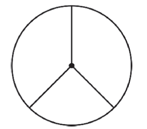
Figure 4: Witten diagram for a three-point function.

From the proposal (2.56) we may calculate connected Green’s functions in the CFT by taking functional derivatives with respect to the sources on both sides of this equation. On the field theory side we have

$$\langle\mathcal{O}_{1}(x_{1})\dots\mathcal{O}_{n}(x_{n})\rangle=-\frac{\delta^{n}W}{\delta\phi^{1}_{(0)}(x_{1})\dots\delta\phi^{n}_{(0)}(x_{n})}\Big{|}_{\phi^{i}_{(0)}=0}\,.$$ (2.57)

Using (2.56) we may thus calculate CFT correlation functions from the propagation of the source fields through AdS space. Since the gravity action is classical, only tree diagrams contribute. The classical propagators on the gravity side are given by the Green’s functions of the operator $\Box_{\mathrm{AdS_{5}}}$, while the vertices are obtained from higher order terms in the Kaluza-Klein reduction of the ten-dimensional gravity fields on $S^{5}$. The corresponding Feynman diagrams are referred to as Witten diagrams [32] . These are usually drawn as a circle depicting the boundary of AdS space, with the interior of the circle corresponding to the AdS bulk space. An example for a Witten diagram leading to a three-point function is shown in figure 4. Here, each of the three lines in the bulk of AdS corresponds to bulk-to-boundary propagator, i.e. to the appropriate Green’s function of $\Box_{\mathrm{AdS_{5}}}$ with one endpoint at the boundary. For scalar operators, the bulk-to-boundary propagator is given by

$$K_{\Delta}(z_{0},\vec{z};\vec{x})=\frac{\Gamma(\Delta)}{\pi^{d/2}\Gamma(\Delta-\frac{d}{2})}\left(\frac{z_{0}}{z_{0}^{2}+(\vec{z}-\vec{x})^{2}}\right)^{\Delta}$$ (2.58)

in Euclidean AdS space with five-dimensional coordinates $z\equiv(z_{0},\vec{z})$ with $z_{0}$ the radial coordinate and $\vec{z}$ the four coordinates parallel to the boundary. For the second coordinate, $x_{0}=0$ since $x$ is located at the boundary. The index $\Delta$ corresponds to the dimension of the dual scalar operator. Moreover, the vertex in the Witten diagram corresponds to a cubic coupling obtained from the Kaluza-Klein reduction of the type IIB supergravity action on $S^{5}$. For four-point functions or even higher correlation functions, there are contributions involving bulk-to-bulk propagators that link two vertices in the bulk of AdS space. The calculation of two- and three point functions of 1/2 BPS operators in ${\cal N}=4$ Super Yang-Mills theory and in IIB supergravity on AdS₅ $\times$ $S^{5}$ provides an impressive test of the AdS/CFT conjecture: The results for the three-point function in field theory and gravity coincide, subject to an appropriate normalization using the expressions for the two-point function [28, 29].

2.5 Finite temperature

Let us now consider how the AdS/CFT correspondence may be generalized to quantum field theory at finite temperature. In fact, there is a natural way to proceed, which is based on the following. In thermal equilibrium, quantum field theories may be described in the imaginary time formalism. This means that the ensemble average of an operator at temperature $T$ is given by

$$\langle{\cal O}\rangle_{\beta}=\mathrm{tr}\left(\frac{\exp(-\beta H)}{Z}\cal{O}\right)\,,\quad Z=\mathrm{tr}\exp(-\beta H)\,,$$ (2.59)

where $\beta=1/(k_{B}T)$ and we set $k_{B}=1$. $H$ is the Hamiltonian of the theory considered. Formally, $\beta$ corresponds to an imaginary time, $t=i\tau$. An important point is that the analyticity properties of thermal Green’s functions require $\tau\in[0,\beta]$. This implies that the imaginary time $\tau$ is compactified on a circle.

Let us consider the gravity dual thermodynamics of ${\cal N}=4$ Super Yang-Mills theory on $I\!\!R^{3}$. We note that the compactification of the time direction breaks supersymmetry, since antiperiodic boundary conditions have to be imposed on the fermions present in the field theory Lagrangian.

The essential point for constructing the gravity dual is that on the gravity side, the field theory described above is identified with the thermodynamics of black D3-branes in Anti-de Sitter space. The solitonic solution for these branes is given by the metric

$$ds^{2}=H(r)^{-1/2}\left(-f(r)dt^{2}+d\vec{x}^{2}\right)\,+\,H(r)^{1/2}\left(\frac{dr^{2}}{f(r)}+r^{2}d\Omega_{5}{}^{2}\right)\,,$$ (2.60)

$$f(r)=1-\left(\frac{r_{H}}{r}\right)^{4}\,,\qquad H(r)=1+\frac{L^{4}}{r^{4}}\,,$$ (2.61)

The blackening factor $f(r)$ vanishes at the Schwarzschild horizon $r_{h}$ of the black brane. The difference between a black brane and a black hole is that the black brane is infinitely extended in the spatial $\vec{x}$ directions, which span $I\!\!R^{3}$. Setting $z=L^{2}/r$, Wick rotating to imaginary time and taking the near-horizon limit as before, this gives

$$ds^{2}=\frac{L^{2}}{z^{2}}\left(\left(1-\frac{z^{4}}{z_{H}^{4}}\right)d\tau^{2}+d\vec{x}^{2}+\frac{1}{1-\frac{z^{4}}{z_{H}^{4}}}dz^{2}\right)+L^{2}d\Omega_{5}^{2}\,,$$ (2.62)

with $z_{H}$ the Schwarzschild radius. As for a black hole, we note that $g_{\tau\tau}\rightarrow 0$, $g_{zz}\rightarrow\infty$ for $z\rightarrow z_{H}$. Let us now introduce a further variable

$$z=z_{H}\left(1-\frac{\rho^{2}}{L^{2}}\right)\,.$$ (2.63)

Here, $\rho$ is a measure for the distance from the horizon at $z_{H}$, outside the black hole. We expand about the horizon. To lowest order in $\rho$, the $(\tau,z)$ contribution to the Euclidean metric becomes

$$ds^{2}\simeq\frac{4\rho^{2}}{z_{H}^{2}}d\tau^{2}+d\rho^{2}\,.$$ (2.64)

With $\phi\equiv 2\tau/z_{H}$, this becomes $ds^{2}=d\rho^{2}+\rho^{2}d\phi^{2}$. For regularity at $\rho=0$, we have to impose that $\phi$ is periodic with period $2\pi$, such that we have a plane rather than a conical singularity. This implies that $\tau$ becomes periodic with period $\Delta\tau=\pi z_{H}$. From the field-theory side we know that $\Delta\tau=\beta=1/T$, which implies

$$z_{H}=\frac{1}{\pi T}.$$ (2.65)

Thus the field-theory temperature is identified with the Hawking temperature of the black brane!

We may now compute the field-theory thermal entropy from the Bekenstein-Hawking entropy of the black brane [33]. In general, the Bekenstein-Hawking entropy is given by the famous result

$$S_{\mathrm{BH}}=\frac{A_{d-1}}{4G_{d+1}}\,,$$ (2.66)

where $A_{d-1}$ is the area of the black brane horizon and $G_{d+1}$ is the Newton constant. For a black D3-brane, the horizon area is given by

$$A_{3} =\int\!d^{3}x\,\sqrt{g_{3d}\Big{|}_{z=z_{H}}}\cdot\mathrm{Vol}(S^{5})\,,\qquad g_{3d}=g_{11}g_{22}g_{33}=\frac{L^{6}}{z^{6}}\,,$$

$$=\pi^{6}L^{8}T^{3}\mathrm{Vol}(\mathbbm{R}^{3})\,,$$ (2.67)

where we used the useful formulae Vol$(S^{5})=\pi^{3}L^{5}$,

$$G_{5}=\frac{G_{10}}{\mathrm{Vol(S^{5})}}=\frac{\pi L^{3}}{2N^{2}}\,,$$ (2.68)

$2\kappa_{10}=16\pi G_{10}=(2\pi)^{7}\alpha^{\prime 4}g_{s}^{2}$ and $L^{4}=4\pi g_{s}N\alpha^{\prime 2}$. Combining all results, we find

$$S_{\mathrm{BH}}=\frac{\pi^{2}}{2}N^{2}T^{3}\mathrm{Vol}(\mathbbm{R}^{3})\,.$$ (2.69)

This result, valid at strong coupling, differs just by its prefactor from the free field theory result

$$S_{\mathrm{free}}=\frac{2\pi^{2}}{3}N^{2}T^{3}\mathrm{Vol}(\mathbbm{R}^{3})\,.$$ (2.70)

We note that the result at strong coupling is smaller by a factor of $3/4$.

3 Holographic Kondo model

As an example of how to generalize the original example of the AdS/CFT correspondence to more general cases, we will now study how to obtain a gravity dual of the well-known Kondo model of condensed matter physics.

The original Kondo model [34] describes the interaction of a free electron gas with a localized magnetic spin impurity. A crucial feature is that at low energies, the impurity is screened by the electrons. The Kondo model is in agreement with experiments involving metals with magnetic impurities, as it correctly predicts a logarithmic rise of the resistivity as the temperature approaches zero.

The significance of the Kondo model goes far beyond its origin as a model for metals with magnetic impurities. In particular, it played a crucial role in the devopment of the renormalization group (RG). The impurity coupling in the Kondo model has a negative beta function and perturbation theory breaks down at low energies, a property it shares with quantum chromodynamics (QCD). In some respects the Kondo model may thus be viewed as a toy model for QCD. Moreover, the Kondo model corresponds to a boundary RG flow connecting two RG fixed points. These correspond to a UV and a IR CFT, respectively. CFT techniques have proved very useful in studying the Kondo model, as reviewed in [35]. Moreover, the Kondo model has a large $N$ limit in which it may be exactly solved using the Bethe ansatz [36, 37, 38].

The holographic Kondo model we will introduce below differs from the original condensed matter model in that the ambient electrons are strongly coupled among themselves even before the interaction with the magnetic impurity isturned on. Moreover, the impurity is an $SU(N)$ spin with $N\rightarrow\infty.$ The ambient degrees of freedom are dual to a gravity theory in an AdS₃ geometry at finite temperature. The impurity degrees of freedom are dual to an AdS₂ subspace. As we will see in detail below, the dual gravity model corresponds to a holographic RG flow dual to a UV fixed point perturbed by a marginally relevant operator, which flows to an IR fixed point. In addition, in the IR a condensate forms, such that the model has some similarity to a holographic superconductor [39]. For this model, we may calculate spectral functions and compare their shape to what is expected for the original Kondo model. This may be relevant for the physics of quantum dots. Including the backreaction of the impurity geometry on the ambient geometry allows to calculate the entanglement entropy. Quantum quenches of the Kondo coupling may also be considered.

3.1 Kondo model within field theory and condensed matter physics

Let us begin by considering the original model of Kondo [34], which describes the interaction of a free electron gas with a $SU(2)$ spin impurity. The electrons are also in the spin 1/2 representation of a second $SU(2)$. Using field-theory language, the corresponding Hamiltonian may be written as

$$H=\frac{v_{F}}{2\pi}i\psi^{\dagger}{\partial}_{x}\psi\,+\,\frac{v_{F}}{2}\lambda_{K}\delta(x)\vec{J}\cdot\vec{S}\,.$$ (3.1)

Here, $v_{F}$ is the Fermi velocity, and $\vec{S}$ is the magnetic impurity satisfying

$$\left[S^{a},S^{b}\right]=i\epsilon^{abc}S^{c}\,,$$ (3.2)

which takes values in the internal $SU(2)$ spin space. The spin impurity interacts with the electron current

$$J^{a}=\psi^{\dagger}\sigma^{a}\psi\,,$$ (3.3)

with $\sigma^{a}$ the Pauli matrices. The Hamiltonian consists of a kinetic term for the electrons and an interaction localized at the site of the impurity. Hence the interaction term involves a delta distribution.

The Kondo model is simplified in the s-wave approximation, where the problem becomes spherically symmetric. We thus introduce polar coordinates $(r,\theta,\phi)$. The dependence on the two angles becomes trivial and we are left with a 1+1-dimensional theory in the space spanned by $(r,t)$. The radial coordinate $r$ runs from zero to infinity. The impurity sits at the origin and provides a boundary condition. The electrons separate into left- and right movers. It is now convenient to analytically continue $r$ to negative values. Then, the previous right-movers become left-movers travelling at negative values of $r$, i.e. $\psi_{R}(r)\rightarrow\psi_{L}(-r)$, as shown in figure 5.

Figure 5: Analytic continuation to negative values of $r$. The right-movers become left-movers travelling at negative values of $r$.

The Hamiltonian (3.1) was proposed and solved perturbatively by Jun Kondo [34]. To first order in perturbation theory, the quantum correction to the resistivity is

$$\rho(T)=\rho_{0}\left[\lambda_{K}+\nu\lambda_{K}^{2}\ln\frac{D}{T}+\dots\right]^{2}\,,$$ (3.4)

where $\nu$ is the density of states and $D$ a UV cut-off, for instance the bandwidth. The corresponding Feynman graph is shown in figure 6.

Figure 6: One-loop Feynman graph contributing to the renormalization of the Kondo coupling, with an electron (solid line) scattering off the impurity (dashed line).

This correction explains the experimental result for a logarithmic rise at low temperatures. From a theoretical perspective, we note that perturbation theory breaks down at a temperature scale

$$T_{K}=D\,\exp\left(-\frac{1}{\nu\lambda_{K}}\right)\,,$$ (3.5)

which defines the Kondo temperature $T_{K}$. At this scale, the first order perturbative correction is of the same order as the zeroth order term, which implies that perturbation theory breaks down.

For the coupling itself, the first order perturbative correction gives the beta function

$$\beta(\lambda_{K})_{\mathrm{one-loop}}=T\frac{d\lambda_{K}}{dT}=-\nu\lambda_{K}^{2}\,.$$ (3.6)

So the beta function is negative. This is analogous to the gauge beta function in QCD, which is also negative - a property associated with asymptotic freedom in the UV. By analogy, we see that the Kondo temperature $T_{K}$ plays a similar role as the scale $\Lambda_{\mathrm{QCD}}$ in QCD, at which perturbation theory breaks down.

A resummation of (3.6) leads to the effective coupling

$$\lambda_{\mathrm{eff}}(T)=\frac{\lambda_{K}}{1-\nu\lambda_{K}\ln(D/T)}\,.$$ (3.7)

$\lambda_{\mathrm{eff}}(T)$ diverges at $T\sim T_{K}=D\exp(-1/(\nu\lambda_{K}))$. In the IR for $T\rightarrow 0$, the theory has a strongly coupled fixed point where the effective coupling vanishes. In fact, the impurity is screened: The impurity spin forms a singlet with the electron spin,

$$|\psi\rangle=\frac{1}{\sqrt{2}}\left(|\Uparrow\downarrow\rangle-|\Downarrow\uparrow\rangle\right)\,.$$ (3.8)

This is reminiscent of the formation of meson bound states in QCD.

The theories at the UV and IR fixed points of the flow are described by boundary conformal field theories (bCFT). Using the analytic continuation described above, In the UV, the theory is free, and we may impose the boundary condition $\psi_{L}(0)=\psi_{R}(0)$ for the left- and right moving electrons introduced above. In the IR however, due to the screening it costs energy to add a further electron to the singlet at $r=0$. The probability for an electron to be at $r=0$ in the ground state is zero. This observation is encoded in the antisymmetric boundary condition $\psi_{R}(0)=-\psi_{L}(0)$. Within bCFT, the Kondo model was analyzed extensively by Affleck and Ludwig [40], making non-trivial use of the appropriate representations of the conformal and the spin Kac-Moody algebra.

Both the UV and the non-trivial IR fixed point of the Kondo RG flow may be described using CFT techniques. Essentially, the interaction may be translated into a boundary condition at $r=0$. Let us sketch this approach, considering a general $SU(N)$ spin group instead of the $SU(2)$ considered above, as well as $k$ species (also called channels or flavours) of electrons. In the UV, the boundary condition relating the left- and right movers is just $\psi_{L}(0)=\psi_{R}(0)$. In the IR, a bound state involving the impurity spin forms, which is a singlet when $N=k=2$. This implies that it costs energy to add another electron at $r=0$, and the probability of finding another electron there is zero. This is described by an antisymmetric wave function as provided by the boundary condition $\psi_{L}(0)=-\psi_{R}(0)$.

It may be shown [35] that by introducing the currents

$$J_{\mathrm{charge}}=:\psi^{\dagger\,\alpha i}\psi_{\alpha i}:\,,\qquad J^{a}_{\mathrm{spin}}=:\psi^{\dagger\alpha i}T^{a}_{\alpha}{}^{\beta}\psi_{\beta i}:\,,\qquad J^{A}_{\mathrm{channel}}=:\psi^{\dagger\alpha i}\tau^{A}_{i}{}^{j}\psi_{\alpha j}:\,,$$ (3.9)

where the colon denotes normal ordering, $T^{a}_{\alpha}{}^{\beta}$ are $SU(N)$ generators and $\tau^{A}_{i}{}^{j}$ are $SU(k)$ generators, the Kondo Hamiltonian may be written as

$$H=\frac{1}{2\pi(N+k)}J^{a}_{\mathrm{spin}}J^{a}_{\mathrm{spin}}+\frac{1}{2\pi(k+N)}J^{A}_{\mathrm{channel}}J^{A}_{\mathrm{channel}}+\frac{1}{4\pi Nk}(J_{\mathrm{charge}})^{2}+\lambda_{K}\delta(r)S^{a}J^{a}_{\mathrm{spin}}\,.$$ (3.10)

In the IR, by writing

$$\mathcal{J}^{a}_{\mathrm{spin}}=J^{a}_{\mathrm{spin}}+\lambda_{K}\delta(r)S^{a}\,,$$ (3.11)

the interaction term may be absorbed into a new current $\mathcal{J}^{a}_{\mathrm{spin}}$. Written in terms of this new current, the Hamiltonian again reduces to the Hamiltonian of the free theory without interaction. The interaction is thus absorbed and replaced by the non-trivial boundary condition discussed above.

At the conformal fixed points, the spin, channel and charge currents may be expanded in a Laurent series,

$$J^{a}(z)=\sum\limits_{n\in\mathbbm{Z}}z^{-n-1}J^{a}_{n}\,.$$ (3.12)

The mode expansions then satisfy Kac-Moody algebras,

$$[J^{a}_{n},J^{b}_{m}]=if^{abc}J^{c}_{n+m}+\frac{n}{2}k\delta^{ab}\delta_{m+n,0}\,,$$ (3.13)

as shown here for the spin current with $SU(N)_{k}$ symmetry, where $k$ denotes the level of the Kac-Moody algebra. Similarly, for the channels we have a $SU(k)_{N}$ symmetry. The total symmetry of the model is $SU(N)_{k}\times SU(k)_{N}\times U(1)$. The representations of the two Kac-Moody algebras are fused in a tensor product. The two different boundary conditions in the UV and in the IR lead to different representations and thus operator spectra for the total theory.

In the simplest example when the spin is $s=1/2$ and there is only one species of electrons, $k=1$, then in the IR a singlet forms. More generally, a singlet is present when $2s=k$, which is referred to as critical screening. When $k<2s$, however, the impurity has insufficient channels to screen the impurity completely, and there is a residual spin of size $|s-k/2|$. This is referred to as underscreening. On the other hand, when $k>2s$ there are too many electron species for a critical screening of the spin, which leads to non-Fermi liquid behaviour, a situation called overscreening.

3.2 Large $N$ Kondo model

As was found by condensed matter physicists in the eighties [41, 42], the Kondo model simplifies considerably when the rank $N$ of the spin group is taken to infinity. In this limit, the interaction term $\vec{J}\cdot\vec{S}$ reduces to a product $\mathcal{OO}^{\dagger}$ involving as scalar operator $\mathcal{O}$, and the screening corresponds to the condensation of $\mathcal{O}$. For comparison to gauge/gravity duality, it will be useful to consider this large $N$ solution in which the Kondo screening appears as a condensation process in $0+1$ dimensions. In the large $N$ limit, a phase transition is possible in such low dimensions since long-range fluctuations are suppressed. Moreover, there is an alternative large $N$ solution of the Kondo model using the Bethe ansatz [36, 37].

The large $N$ limit of the Kondo model involves $N\rightarrow\infty$, $\lambda\rightarrow 0$ with $\lambda N$ fixed. The vector large $N$ limit of the Kondo model provides information about the spectrum, thermodynamics and transport properties everywhere along the RG flow, even away from the fixed points. $1/N$ corrections may be calculated.

We consider totally antisymmetric representations of $SU(N)$ given by a Young tableau consisting of one column with $q$ boxes, $q<N$. We write the spin in terms of Abrikosov pseudo-fermions $\chi$, which means that we consider

$$S^{a}=\chi^{\dagger}{}^{i}T^{a}{}_{i}{}^{j}\chi_{j}\,,\qquad a=1,2,\dots,N^{2}-1\,,$$ (3.14)

with $\chi$ in the fundamental representation of $SU(N)$. A state in the impurity Hilbert space is obtained by acting on the vacuum state with $q$ of the $\chi^{\dagger}$. This gives rise to a totally antisymmetric tensor product with rank $q$. Since (3.14) is invariant under phase rotations of the $\chi$’s, there is an additional new $U(1)$ symmetry. This implies that we need to impose a constraint since considering the $\chi$’s instead of $S^{a}$ should not introduce any new degrees of freedom. We impose

$$\chi^{\dagger}\chi=q\,,$$ (3.15)

i.e. the charge density of the Abrikosov fermions is given by the size of the totally antisymmetric representation. Together with the fermions $\psi$ of the Kondo model, we have a $SU(N)$ singlet operator

$$\mathcal{O}(t)\equiv\psi^{\dagger}\chi\,,\qquad\Delta_{\mathcal{O}}=\frac{1}{2}\,.$$ (3.16)

Now in the large $N$ limit, the Kondo interaction $\vec{J}\cdot\vec{S}$ simplifies considerably as follows. We make use of the Fierz identity (2.20). For the Kondo interaction this implies

$$\lambda\delta(x)J^{a}S^{a}=\lambda\delta(x)(\psi^{\dagger}T^{a}\psi)(\chi^{\dagger}T^{a}\chi)=\frac{1}{2}\lambda\delta(x)\left(\mathcal{O}\mathcal{O}^{\dagger}-\frac{q}{N}(\psi^{\dagger}\psi)\right)\,,$$ (3.17)

where for sufficiently small $q$ we may neglect the last term in the limit $N\rightarrow\infty$.

In the large $N$ limit, the Kondo coupling is thus the coupling of a‘double-trace’ deformation $\mathcal{OO}^{\dagger}$, with two separately gauge invariant operators $\mathcal{O}$ and $\mathcal{O}^{\dagger}$. This is similar to double-trace operators where two separately gauge-invariant operators are multiplied to each other. For operators involving fields in the adjoint representation, traces have to be taken to generate gauge-invariant operators. Here however, $\mathcal{O}$ is gauge invariant without trace, since both $\psi$ and $\chi$ are in the fundamental of $SU(N)$. The operator $\mathcal{OO}^{\dagger}$ is of engineering dimension one. As defect operator, it is marginally relevant, i.e. it is marginal at the classical level, but quantum corrections make it relevant.

In the large $N$ limit, the solution of the field-theory saddle point equations reveals a second order mean-field phase transition in which $\mathcal{O}$ condenses: There is a critical temperature $T_{c}$ above which $\langle\mathcal{O}\rangle=0$ and below which $\langle\mathcal{O}\rangle\neq 0$. The critical temperature $T_{c}$ is slightly smaller than the Kondo temperature $T_{K}$ and may be calculated analytically. The condensate spontaneously breaks the $U(1)$ symmetry of the $\chi$ fermions. $1/N$ corrections smoothen this transition to a cross-over.

At large $N$, the Kondo model thus has similarity with superconductivity that is triggered by a marginally relevant operator. This observation provides a guiding principle for constructing a gauge/gravity dual of the large $N$ Kondo model.

3.3 Gravity dual of the Kondo model

The motivation of establishing a gravity dual of the Kondo model is twofold: On the one hand, this provides a new application of gauge/gravity duality of relevance to condensed matter physics. On the other hand, this provides a gravity dual of a well-understood field theory model with an RG flow, which may provide new insights into the working mechanisms of the duality. It is important to note that our holographic Kondo model will have some features that are distinctly different from the well-known field theory Kondo model described above. Most importantly, the 1+1-dimensional electron gas will be strongly coupled even before considering interactions with the impurity. This has some resemblance with a Luttinger liquid coupled to a spin impurity. Moreover, the $SU(N)$ spin symmetry will be gauged. The holographic Kondo model has provided insight into the entanglement entropy of this system. Moreover, quenches of the Kondo coupling in the holographic model provide a new geometric realization of the formation of the Kondo screening cloud. It is conceivable that further work will also lead to new insight into the Kondo lattice that involves a lattice of magnetic impurities. The Kondo lattice is a major unsolved problem within condensed matter physics. Preliminary results in this direction that were obtained using holography may be found in [43]. Further holographic studies of holographic Kondo models include [44].

Here we aim at constructing a holographic Kondo model realizing similar features to the ones of the large $N$ field theory Kondo model described in the previous section, including a RG flow triggered by a doulbe-trace operator [45]. For this purpose, consider an appropriate configuration of D-branes which allows us to realize the field theory operators needed. The field theory involves fermionic fields $\psi$ in 1+1 dimensions in the fundamental representation of $SU(N)$, as well as Abrikosov fermion fields $\chi$ localized at the 0+1-dimensional defect. These transform in the fundamental representation of $SU(N)$ as well. From these we will construct the required operators. For the brane configuration we will use probe branes, which means that a small number of coincident branes are embedded into a D3-brane background, neglecting the backreaction on the geometry. For a holographic Kondo model, a suitable choice of probe branes consists of D7- and D5-branes embedded as shown in table 4.

	0	1	2	3	4	5	6	7	8	9
$N$ D3	X	X	X	X
$1$ D7	X	X			X	X	X	X	X	X
$1$ D5	X				X	X	X	X	X

Table 4: Brane configuration for a holographic Kondo model.

Fields in the fundamental representation are obtained from strings stretching between the D3-, D5- and D7-branes. The D7-brane probe extends in 1+1 dimensions of the worldvolume of the D3-branes. As we discuss below, strings stretching between the D3- and D7-branes give rise to chiral fermions, which we identify with the electrons of the Kondo model. On the other hand, since the D5-brane only shares the time direction with the D3-branes, the D3-D5 strings give rise to the 0+1 dimensional Abrikosov fermions.

We note that in a in absence of the D5-branes, the D3/D7-brane system has eight ND directions, such that half of the original supersymmetry is preserved. However, the D5/D7-system has only two ND directions, such that supersymmetry is broken. This leads to the presence of a tachyon potential and a condensation as required for the large $N$ Kondo model. The tachyon, a complex scalar field $\Phi$, is identified as the gravity dual of the operator $\mathcal{O}=\psi^{\dagger}\chi$.

As discussed in [46, 47], the D7-brane gives rise to an action

$$S_{7}=\frac{1}{\pi}\int d^{2}x\psi_{L}^{\dagger}(i{\partial}_{-}-A_{-})\psi_{L}$$ (3.18)

of chiral fermions which are coupled to the ${\cal N}=4$ supersymmetric gauge theory in 3+1 dimensions. $A_{-}$ is a restriction of a component of the ${\cal N}=4$ Super Yang-Mills gauge field to the subspace of the fermions. These fermions are in the fundamental representation of the gauge group $SU(N)$. For simplicity, from now on we drop the label $L$ for left-handed. The gauge field $A_{-}$ is a component of the ${\cal N}=4$ theory gauge field on the 1+1-dimensional subspace spanned by the D7-brane. We identify the $\psi_{L}$ with the electrons of the Kondo model.

Similarly, for the Abrikosov fermions $\chi$ we obtain from the D3/D5-brane system the action

$$S_{5}=\int dt\chi^{\dagger}(i{\partial}_{t}-A_{t}-\Phi_{9})\chi\,.$$ (3.19)

Here, $\Phi_{9}$ is the adjoint scalar of ${\cal N}=4$ Super Yang-Mills theory whose eigenvalues represent the positions of the D3-branes in the $x^{9}$ direction. In (3.19), both $A_{t}$ and $\Phi_{9}$ are restricted to the subspace of the $\chi$ fields. Note that unlike the original Kondo model, the $SU(N)$ spin symmetry is gauged in this approach. Also, the background ${\cal N}=4$ theory is strongly coupled in the gravity dual approach and provides strong interactions between the electrons.

Let us now turn to the gravity dual of this configuration. The $N$ D3-branes provide an AdS₅ $\times$ $S^{5}$ supergravity background as before. The probe D7-brane wraps an AdS₃ $\times$ $S^{5}$ subspace of this geometry, while the probe D5-branes wraps AdS₂ $\times$ $S^{4}$. The Dirac-Born-Infeld action for the D5-brane contains a gauge field $a_{\mu}$ on the AdS₂ subspace spanned by $(t,r)$, with $t$ the time coordinate and $r$ the radial coordinate in the AdS geometry. The $a_{t}$ component of this gauge field is dual to the charge density of the Abrikosov fermions, $q=\chi^{\dagger}\chi$. The D7-brane action contains a Chern-Simons term for a gauge field $A_{\mu}$ on AdS₃. As noted before, the D5-D7 strings lead to a complex scalar tachyon field.

We may thus establish the holographic dictionary for the operators of the field-theory large $N$ Kondo model given in table 5. The electron current in 1+1 dimensions is dual to the Chern-Simons field in 2+1 dimensions. The Abrikosov fermion charge density $q$ in 0+1 dimensions is dual to the gauge field component $a_{t}$ in 1+1 dimensions. Finally, the operator $\mathcal{O}=\psi^{\dagger}\chi$ in 0+1 dimensions is dual to the complex scalar field $\Phi$ in 1+1 dimensions.

Operator		Gravity field
Electron current $J^{\mu}=\bar{\psi}\gamma^{\mu}\psi$	$\Leftrightarrow$	Chern-Simons gauge field $A$ in $AdS_{3}$
Charge density $q=\chi^{\dagger}\chi$	$\Leftrightarrow$	2d gauge field $a$ in $AdS_{2}$
Operator ${\cal O}=\psi^{\dagger}\chi$	$\Leftrightarrow$	2d complex scalar $\Phi$ in AdS2

Table 5: Field-operator map for the holographic Kondo model.

The brane picture has allowed us to neatly establish the required holographic dictionary. Unfortunately, it is extremely challenging to derive the full action describing the brane construction given. In particular, the exact form of the tachyon potential is not known.

For making progress towards describing a variant of the Kondo model holographically, we thus turn to a simplified model consisting of a Chern-Simons field in AdS₃ coupled to a Yang-Mills gauge field and a complex scalar in AdS₂. This simplification still allows us to use the holographic dictionary established above. The information we lose though is about the full field content of the strongly coupled field theory. On the other hand, this simplifield model allows for explicit calculations of observables such as two-point functions and the impurity entropy, as we discuss below. It is instructive to compare the results of these calculations with features of the field-theory large $N$ Kondo model, as we shall see.

The simplified model we consider is

$$S= \frac{1}{8\pi G_{N}}\int dzdxdt\sqrt{-g}\,(R-2\Lambda)-\frac{N}{4\pi}\int\limits_{\mathrm{AdS}_{3}}A\wedge{d}A$$

$$-N\int dxdt\sqrt{-g}\left(\frac{1}{4}\mathrm{tr}f^{mn}f_{mn}+(D^{m}\Phi)^{\dagger}(D_{m}\Phi)-V(\Phi)\right)\,.$$ (3.20)

Here, $z$ is the radial AdS coordinate, $x$ is the spatial coordinate along the boundary and $t$ is time. The defect sits at $x=0$. The first term is the standard Einstein-Hilbert action with negative cosmological constant $\Lambda$. The second term is a Chern-Simons term involving the gauge field $A_{\mu}$ dual to the electron current $J^{\mu}$. We take $A_{\mu}$ to be an Abelian gauge field, which implies that we consider only one flavour of electrons, or - in condensed matter vterms - only one channel. $f_{mn}$ is the field strength tensor of the gauge field $a_{m}$ with $m\in\{t,z\}$, which we take to be Abelian too. Its time component $a_{t}$ is dual to the charge density $\psi^{\star}\psi$, which at the boundary takes the value $Q=q/N$ with $q$ the dimension of the antisymmetric prepresentation of the spin impurity. $D_{m}$ is a covariant derivative given by $D_{m}={\partial}_{m}+iA_{m}\Phi-ia_{m}\Phi$. For the complex scalar, we assume its potential to take the simple form

$$V(\Phi^{\dagger}\Phi)=M^{2}\Phi^{\dagger}\Phi\,.$$ (3.21)

We write the complex field as $\Phi=\phi\exp{i\delta}$ with $\phi=|\Phi|$. We choose $M^{2}$ in such a way that $\Phi^{\dagger}\Phi$ is a relevant operator in the UV limit. It becomes marginally relevant when perturbing about the fixed point. Moreover, for the time being we consider the matter fields as probes, such that they do not influence the background geometry. For this background geometry we take the solution to the gravity equations of motion which corresponds to the AdS BTZ black hole, i.e.

$$ds^{2}_{\mathrm{BTZ}}=\frac{1}{z}\left(\frac{1}{h(z)}dz^{2}-h(z)dt^{2}\right)\,,$$

$$h(z)=1-\frac{z^{2}}{z_{h}^{2}}\,,$$ (3.22)

where we set the AdS radius to one, $L=1$, and $z_{h}$ is related to the temperature by

$$T=\frac{1}{2\pi z_{h}}\,.$$ (3.23)

The non-trivial equations of motion for the matter fields are given by

$${\partial}_{z}A_{x}=4\pi\delta(x)\sqrt{g}g^{tt}a_{t}\phi^{2}\,,$$

$${\partial}_{z}(\sqrt{-g}g^{zz}g^{tt}{\partial}_{z}a_{t})=2\sqrt{-g}g^{tt}a_{t}\phi^{2}\,,$$

$${\partial}_{z}(\sqrt{-g}g^{zz}{\partial}_{z}\phi)=\sqrt{-g}g^{tt}a_{t}^{2}\phi+\sqrt{-g}M^{2}\phi\,.$$ (3.24)

The three-dimensional gauge field $A_{\mu}$ is non-dynamical, but will be responsible for a phase shift similar to the one observed in the field-theory Kondo model.

Above the critical temperature $T_{c}$ where $\mathcal{O}$ dual to the scalar field condenses, we have $\phi=0$. Then, asymptotically near the boundary, we have $a_{t}(z)\sim\frac{Q}{z}+\mu$, where $\mu$ is a chemical potential for the spurious $U(1)$ symmetry rotating the $\chi$’s. The charge density is given by $\chi^{\dagger}\chi=NQ$, with $Q=q/N$.

For generating the Kondo RG flow, we need to turn on the marginally relevant ‘double-trace’ operator ${\mathcal{O}}{\mathcal{O}^{\dagger}}$. We choose the mass $M$ in the potential such that the field $\phi(z)$ is at the Breitenlohner-Freedman stability bound [48]. The asymptotic behaviour of $\phi(z)$ near the boundary is then

$$\phi(z)=\alpha z^{1/2}\ln(\Lambda z)-\beta z^{1/2}+{\cal O}(z^{3/2}\ln(\Lambda z)\,.$$ (3.25)

Following [49, 50], the gravity dual of a double-trace perturbation is obtained by imposing a linear relation between $\alpha$ and $\beta$,

$$\alpha=\kappa\beta\,.$$ (3.26)

We choose $\alpha$ to correspond to a source for the operator ${\cal O}$, while $\beta$ is related to is vacuum expectation value. The physical coupling $\phi(z)$ should be a RG invariant, i.e. invariant under changes of the cut-off $\Lambda$. This implies

$$\kappa=\frac{\kappa_{0}}{1+\kappa_{0}\ln(\Lambda_{0}/\Lambda)}\,.$$ (3.27)

At finite temperature, we obtain the analogous result

$$\kappa_{T}=\frac{\kappa_{0}}{1+\kappa_{0}\ln(\Lambda z_{h})}$$ (3.28)

This expression for the coupling $\kappa_{T}$ diverges at the temperature

$$T_{K}=\frac{1}{2\pi}\Lambda e^{1/\kappa_{0}}\,,$$ (3.29)

where $T_{K}$ is the Kondo temperature. A similar behaviour is observed in the condensed matter Kondo models. Moreover, this behaviour bears some similarity to QCD, where the coupling becomes strong at a scale $\Lambda_{\mathrm{QCD}}$, below which bound states provide the natural description of the degrees of freedom. Of course, in the holographic Kondo model there are two couplings, one between the electrons themselves and secondly the Kondo coupling $\kappa_{T}$. While the first is strong along the entire flow, $\kappa_{T}$ diverges at the Kondo temperature and then becomes small again at lower temperatures, where the condensate forms.

For determining the physical properties of the model considered, we have to resort to numerics to solve the equations of motion (3.24). We find a mean-field phase transition as expected for a large-$N$ theory, as shown in figure 7. In the screened phase, a condensate of the operator ${\cal O}=\psi^{\dagger}\chi$ forms. We note that for very small temperatures, the numerical solution of the equations of motion becomes extremely time-consuming and thus our results are less accurate in this regime. We expect that in the limit $T\rightarrow 0$, to obtain a stable constant solution for $\langle\mathcal{O}\rangle$ requires to add a quartic term to the potential (3.21).

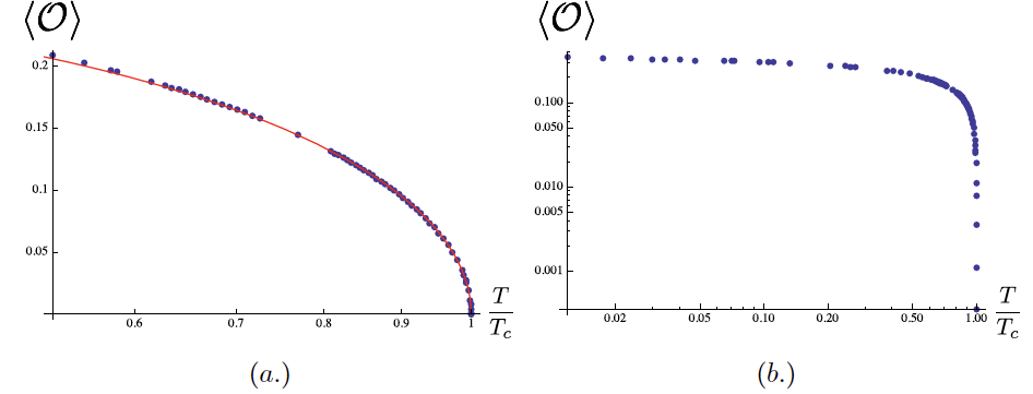
Figure 7: Expectation value of the operator $\mathcal{O}=\psi^{\dagger}\chi$ as function of the temperature. Below $T_{c}$, a condensate forms. (a.) Close to the transition temperature, displaying that the phase transition is mean-field; (b.) Log-log plot showing a larger temperature range. The VEV appears to approach a constant at low temperatures, however further stabilisation by a quartic potential contribution is expected to be required in the limit $T\rightarrow 0$. Figures from [45].

Our holographic model allows for a geometrical description of the screening mechanism in the dual strongly-coupled field theory. For this we consider the electric flux $\mathcal{F}$ of the AdS₂ gauge field $a_{t}(z)$. At the boundary of the holographic space, this flux encodes information about the impurity spin representation,

$$\lim\limits_{z\rightarrow 0}{\cal F}=\lim_{z\rightarrow 0}\sqrt{-g}f^{zt}=a^{\prime}_{t}(z)|_{z\rightarrow 0}=Q\,,$$ (3.30)

with $Q=q/N$ and $q$ as in (3.15). When $\phi=0$, this flux is a constant and takes the same value at the black hole horizon. However for $T<T_{c}$, the non-trivial profile $\phi(z)$ draws electric charge away from $a_{t}(z)$, reducing the electric flux at the horizon. This implies that the effective number of impurity degrees of freedom is reduced, which corresponds to screening. This is shown in figure 8 which shows the flux ${\cal F}_{z\rightarrow z_{h}}$ at the horizon as a function of temperature. The numerical solution of the equations of motion yields a decreasing flux when the temperature is decreased.

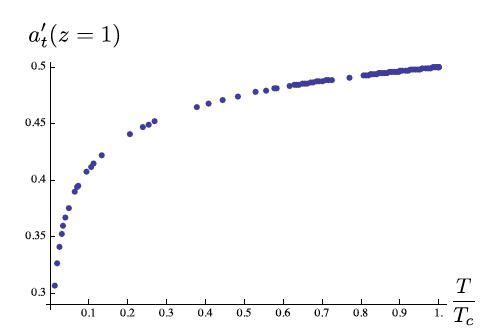
Figure 8: Electric flux through the boundary of AdS₂ at the black hole horizon. This is a measure for the number of degrees of freedom. Its decrease at low temperatures indicates that the impurity is screened. For $T/T_{c}\lesssim 0.2$, the decrease is only logarithmic. The radial variable is normalized such that $z=1$ at the horizon. Figure from [45].

The temperature dependence of the resistivity may be obtained by an analysis of the leading irrelevant operator at the IR fixed point, i.e. by perturbing about the IR fixed point by this operator. This gives $\rho(T)\propto T^{\gamma}$ with $\gamma\in\mathbbm{R}$ a real number. A similar behaviour occurs also in Luttinger liquids [51]. The model thus does not reproduce the logarithmic rise of the resistivity with decreasing temperature observed in the original Kondo model. This behaviour is expected since the model is at large $N$ and the ambient electrons are strongly coupled.

Let us emphasize again the differences between the holographic Kondo model considered here and the large $N$ Kondo model of condensed matter physics: Here, the electrons are strongly coupled among themselves even before coupling them to the spin defect. The system thus has two couplings: the electron-electron coupling which is always large, and the Kondo coupling to the defect that triggers the RG flow. Moreover, we point out that in our model, the $SU(N)$ symmetry is gauged, while it is a global symmetry in the condensed matter models.

To conclude, let us consider different applications of the holographic Kondo model we introduced. These involve three aspects: the impurity entropy, quantum quenches and correlation functions.

3.4 Applications of the holographic Kondo model

3.4.1 Entanglement entropy

The concept of holographic entanglement entropy introduced by Ryu and Takayanagi in 2006 has proved to be an important ingredient to the holographic dictionary [52], opening up new relations between gauge/gravity duality and quantum information. In general, the entanglement entropy is defined for two Hilbert spaces $\mathcal{H}_{A}$ and $\mathcal{H}_{B}$. In the AdS/CFT correspondence, it is useful to consider $A$ and $B$ to be two disjunct space regions in the CFT. Defining the reduced density matrix to be

$$\rho_{A}={\mathrm{tr}}_{B}\rho\,,$$ (3.31)

where $\rho$ is the density matrix of the entire space, the entanglement entropy is given by its von Neumann entropy

$$S=-{\mathrm{tr}}_{A}\rho_{A}\ln\rho_{A}\,.$$ (3.32)

The entanglement entropy bears resemblance with the black hole entropy since it quantifies the lost information hidden in $B$. Ryu and Takayanagi proposed the holographic dual of the entanglement entropy to be

$$S=\frac{\mathrm{Area}\gamma_{A}}{4G_{d+1}}\,,$$ (3.33)

where $G_{d+1}$ is the Newton constant of the dual gravity space and $\gamma_{A}$ is the area of the minimal bulk surface whose boundary coincides with the boundary of region A. For a field theory in 1+1 dimensions, the region A may be taken to be a line of length $\ell$, and the bulk minimal surface $\gamma_{A}$ becomes a bulk geodesic joining the two endpoints of this line, as shown for the holographic Kondo model in figure 9. We note that for a 1+1-dimensional CFT at finite temperature, with the BTZ black hole as gravity dual, it is found both in the CFT [53] and on the gravity side [52] that the entanglement entropy for a line of length $\ell$ is given by

$$S_{\mathrm{BH}}(\ell)=\frac{c}{3}\ln\left(\frac{1}{\pi\epsilon T}\sinh(2\pi\ell T)\right)\,,$$ (3.34)

with $\epsilon$ a cut-off parameter.

For the Kondo model, a useful quantity to consider is the impurity entropy which is given by the difference of the entanglement entropies in presence and in absence of the magnetic impurity,

$$S_{\mathrm{imp}}=S_{\mathrm{impurity\;present}}-S_{\mathrm{impurity\;absent}}\,.$$ (3.35)

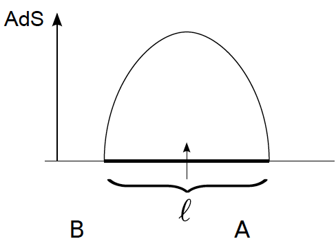
Figure 9: The impurity entropy in the holographic Kondo model is obtained from the entanglement entropy. The entanglement area is a line of length $\ell$ in the dual field theory. The holographic minimal surface is a geodesic. For the impurity entropy, the entanglement entropy in absence of the defect is subtracted from the one in presence of the defect.

In the previous sections, we considered the probe limit of the holographic Kondo model, in which the fields on the AdS₂ defect do not backreact on the AdS₃ geometry. However, including the backreaction is necessary in order to calculate the effect of the defect on the Ryu-Takayanagi surface. A simple model that achieves this [54, 55] consists of cutting the 2+1-dimensional geometry in two halves at the defect at $x=0$ and joining these back together subject to the Israel junction condition [56]

$$K_{\mu\nu}-\gamma_{\mu\nu}K=-\frac{\kappa_{G}}{2}T_{\mu\nu}\,,$$ (3.36)

This procedure is shown in figure 10. We refer to the joining hypersurface as ‘brane’. In (3.36), $\gamma$ and $K$ are the induced metric and extrinsic curvature at the joining hypersurface extending in $(t,z)$ directions. $T_{\mu\nu}$ is the energy-momentum tensor for the matter fields $a$ and $\Phi$ at the defect, and $\kappa_{G}$ is the gravitational constant with $\kappa_{G}^{2}=8\pi G_{N}$.

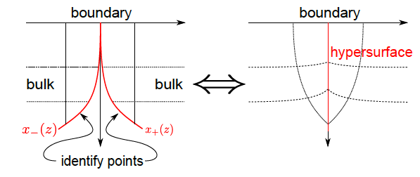
Figure 10: Cutting and joining of two halves of the AdS BTZ geometry subject to the Israel junction at the defect. Figure by Mario Flory.

The matter fields $\Phi$ and $a$ lead to a non-zero tension on the brane, which varies with the radial coordinate. The higher the tension on this brane, the longer the geodesic joining the two endpoints of the entangling interval will be, as shown in figure 11. A numerical solution of the Israel junction condition reveals that the brane tension decreases with decreasing temperature, which leads to a shorter geodesic. This in turn leads to a decrease of the impurity entropy (3.35). This decreases is expected and in agreement with the screening of the impurity degrees of freedom.

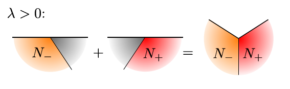
Figure 11: Geometry in a vicinity of the backreacting defect brane at positive brane tension. The horizontal black line corresponds to the boundary of the deformed AdS space, as in figure 10. The volume is increased in a given region around the defect as compared to the case when the brane tension vanishes. This will lead to a longer geodesic for a given entanglement interval and thus to a non-zero positive impurity entropy. Figure by Mario Flory.

In the holographic Kondo model, the brane is actually curved since the brane tension depends on the radial coordinate. For large entangling regions $\ell$, we may approximate the impurity entropy to linear order by noting that the length decrease of the Ryu-Takayanagi geodesic $\gamma_{A}$ translates into a decrease of the entangling region $\ell$ itself. To linear order, this implies that the entangling region is given by $\ell+D$ in the UV and by $\ell$ in the IR, for $D\ll\ell$. Using (3.34) we may thus write for the difference of the impurity between its UV and IR values

$$\Delta S_{\mathrm{imp}} =S_{\mathrm{BH}}(\ell+D)-S_{\mathrm{BH}}(\ell)$$

$$\simeq D\cdot{\partial}_{\ell}S_{\mathrm{BH}}(\ell)=\frac{2\pi DT}{3}\coth(2\pi\ell T)\,.$$ (3.37)

It is a non-trivial result that subject to identifying the scale $D$ with the Kondo correlation length of condensed matter physics, $D\propto\xi_{K}$, then the result agrees with previous field-theory results for the Kondo impurity entropy [57, 58].

3.4.2 Quantum quenches

A quantum quench corresponds to introducing a time dependence of the Kondo coupling. On the gravity side, this implies that the equations of motion become partial differential equations (PDEs), since both the dependence on the AdS radial coordinate and on time are relevant. Quenches of the holographic ‘double trace’ Kondo coupling $\kappa_{T}$ were considered in [59]. Figure 12 shows a quench from the unscreened to the screened phase. The system reacts to this quenchof the coupling by forming a condensate. There is a certain time lapse before this happens. It is also noteworthy that the reaction is overdamped, i.e. there are no oscillations around the new equilibrium value. This behaviour follows from the structure of the quasinormal modes, i.e. the eigenmodes of the gravity system. The leading eigenmode is purely imaginary in this system. This is in agreement with the behaviour of the correlation functions discussed in the next section.

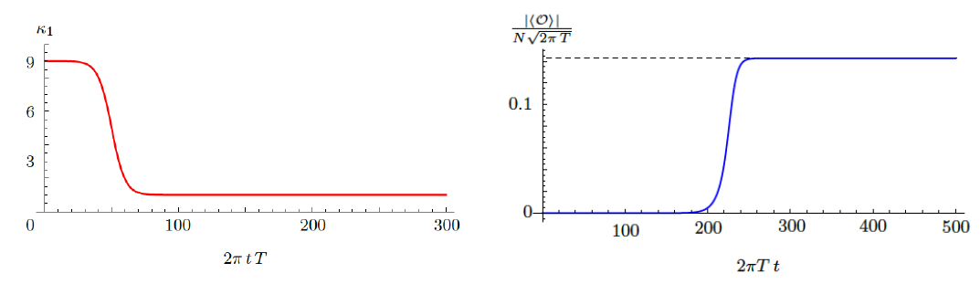
Figure 12: Left: Quench of the ‘double-trace’ Kondo coupling from the unscreened to the screened phase. Right: Reaction of the system to this quench: A condensate forms. There are no oscillations about the new equilibrium configuration. Figure from [59].

3.4.3 Correlation functions

AdS/CFT allows to calculate retarded Green’s functions by adapting the methods presented in section 2.4.3 to Lorentzian signature [60]. The required causal structure is obtained by imposing infalling boundary conditions on the gravity field fluctuations at the black hole horizon. Moreover, a careful regularization using the methods of holographic regularization [61] is essential. This approach was used in [62, 63] to calculate spectral functions for the Kondo operator $\mathcal{O}=\psi^{\dagger}\chi$ of (3.16). Spectral functions are generally obtained from the retarded Green’s function by virtue of

$$\rho(\omega)=-2\,\mathrm{Im}\,G_{R}(\omega)\,.$$ (3.38)

The spectral function measures the number of degrees of freedom present at a given energy. The results for the holographic Kondo model obtained in [62, 63] are shown in figure 13.

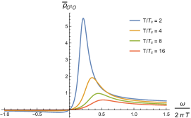
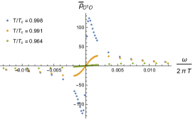
Figure 13: Spectral function $\rho(\omega)$ for the Kondo operator $\mathcal{O}$ at the defect, as function of the frequency $\omega$. a) Left: In the unscreened phase above $T_{c}$. The spectral function corresponds to a Fano resonance with a spectral asymmetry. b) Right: In the screened phase below $T_{c}$. The spectral function is antisymmetric. The Green’s functions’ poles leading to the extrema in $\rho(\omega)$ are determined by the size of the condensate for $\mathcal{O}$. Figures from [62].

Above the critical temperature, these spectral functions show a spectral asymmetry related to a Fano resonance [64]. In the holographic case, this asymmetry is characteristic of the interaction between the ambient strongly coupled CFT and the localized impurity degrees of freedom. A similar spectral asymmetry also appears in the condensed-matter large $N$ Kondo model (which involves free electrons) at vanishing temperature [65]. In the screened phase, the holographic spectral function displayed in figure 13 is antisymmetric, consistent with the relation

$$\omega_{P}\propto-i|\langle\mathcal{O}\rangle|^{2}$$ (3.39)

between the condensate and the leading pole $\omega_{P}$ in the retarded Green’s function. This relation is also satisfied by the condensed matter large-$N$ Kondo model involving free electrons [66].

A similar spectral asymmetry also arises in the context of the Sachdev-Ye-Kitaev (SYK) model that received a lot of attention recently [67, 68]. In fact, the original variant of this model due to Sachdev and Ye [67] involves Weyl fermions, as opposed to the Majorana fermions of the SYK model. This Sachdev-Ye may be obtained from the Ising model by the same mechanism as discussed in (3.14) above, i.e. by writing the Ising spin in terms of a bilinear of auxiliary fermions. In this case, the Ising model is given by

$$H_{S}=-\frac{1}{\sqrt{N}}\sum\limits_{A<B}J_{A,B}{S}^{aA}{S}^{aB}\,,\qquad S^{a}=\psi^{\dagger}T^{a}\psi\,,$$ (3.40)

where the $A,B$ label the different sites of the Ising lattice, and the index $a$ refers to spin space as in (3.14). We see that inserting the fermion bilinear expression for $S^{a}$ into the Ising model will give rise to a four-fermion model. Indeed, as explained in [67, 69], reducing (3.40) to a single-site model by averaging over disorder, and taking the large $N$ limit, gives rise to the Sachdev-Ye model

$$H_{SY}=\frac{1}{(2N)^{3/2}}\sum\limits_{i,j,k,l=1}^{N}\overline{J_{ij,kl}}\,\chi^{\dagger i}\chi^{j}\chi^{\dagger k}\chi^{l}-\mu\sum_{i}\chi^{\dagger i}\chi^{i}\,,$$ (3.41)

where the second term involving the chemical potential $\mu$ is added to fix the representation $q$ of the spin impurity. As discussed in [70], the Sachdev-Ye model also displays a spectral asymmetry. This asymmetry is of an analogous form to the one found above for the holographic Kondo model. In [70], it is shown that the spectral asymmetry in the Sachdev-Ye model may be mapped to the entropy of a black hole in AdS₂ space. A similar mechanism is expected to be at work in the holographic Kondo model introduced above.

4 Conclusion and outlook

Though the concept of duality has existed for some time within theoretical physics, the AdS/ CFT correspondence and its generalizations to gauge/gravity duality are truly remarkable since they relate a theory with gravity to a quantum theory without gravity. This certainly added many new viewpoints on fundamental questions such as the nature of quantum gravity. On this basis, further significant progress is expected within the next couple of years, one particular avenue being the quantum physics of black holes and its relation to quantum information. This provides a striking example of new developments in physics triggered by joining different research areas that previously appeared as unrelated. Equally striking is the new relation between fundamental and practical questions provided by gauge/gravity duality, as it provides a new approach for studying questions in strongly coupled quantum systems. This has been applied to fields as diverse as elementary particle, nuclear and condensed matter physics.

The holographic Kondo model demonstrates nicely how the original concept of the AdS/CFT conjecture may be applied to more involved configurations, in this case involving a marginally relevant perturbation by a ‘double-trace’ operator and a condensation process. It also demonstrates that holographic models may be linked to previous results, in this case the large $N$ Kondo model of condensed matter physics. On the other hand, they also add new features, in this case the coupling of the magnetic impurity to a strongly coupled electron system, leading in particular to new features in quantum quenches and in the spectral function.

The AdS/CFT correspondence and gauge/gravity duality are undoubtedly one of the most exciting developments in physics within the last twenty years. As discussed, new avenues are opening up and are expected to lead to further important discoveries in the future.

5 Acknowledgements

I am grateful to the organizers of TASI 2017, Mirjam Cvetic and Igor Klebanov, for the opportunity to lecture at this lively and inspiring School, and to the participants of TASI 2017 for pertinent questions. Moreover, I would like to thank my co-author Martin Ammon for the joint writing of the book [5] that proved essential for preparing these lectures. I am also grateful to my collaborators on the holographic Kondo project for enjoyable and fruitful joint work: Mario Flory, Carlos Hoyos, Ioannis Papadimitriou, Jonas Probst, Max Newrzella, Andy O’Bannon and Jackson Wu. Last but not least I would like to thank TASI 2017 participant Raimond Abt for proofreading these lecture notes.

References

- [1] S. Coleman, “Quantum sine-Gordon equation as the massive Thirring model,” Phys. Rev. D 11 (1975) 2088–2097.
- [2] C. Montonen and D. Olive, “Magnetic monopoles as gauge particles?,” Physics Letters B 72 (1977) 117–120.
- [3] P. Candelas, G. T. Horowitz, A. Strominger, and E. Witten, “Vacuum configurations for superstrings,” Nuclear Physics B 258 (1985) 46–74.
- [4] J. M. Maldacena, “The Large N limit of superconformal field theories and supergravity,” Int. J. Theor. Phys. 38 (1999) 1113–1133, arXiv:hep-th/9711200 [hep-th]. [Adv. Theor. Math. Phys.2,231(1998)].
- [5] M. Ammon and J. Erdmenger, Gauge/gravity duality: Foundations and applications. Cambridge University Press, Cambridge, 2015.
- [6] H. Nastase, Introduction to the ADS/CFT Correspondence. Cambridge University Press, 2015.
- [7] M. Natsuume, “AdS/CFT Duality User Guide,” Lect. Notes Phys. 903 (2015) pp.1–294, arXiv:1409.3575 [hep-th].
- [8] J. Casalderrey-Solana, H. Liu, K. Mateos, D.and Rajagopal, and U. Wiedemann, Gauge/String Duality, Hot QCD and Heavy Ion Collisions. Cambridge University Press, Cambridge, 2014.
- [9] J. Zaanen, Y.-W. Sun, Y. Liu, and K. Schalm, Holographic Duality in Condensed Matter Physics. Cambridge Univ. Press, 2015.
- [10] I. R. Klebanov, “TASI lectures: Introduction to the AdS / CFT correspondence,” in Strings, branes and gravity. Proceedings, Theoretical Advanced Study Institute, TASI’99, Boulder, USA, May 31-June 25, 1999, pp. 615–650. 2000. arXiv:hep-th/0009139 [hep-th].
- [11] J. M. Maldacena, “TASI 2003 lectures on AdS / CFT,” in Progress in string theory. Proceedings, Summer School, TASI 2003, Boulder, USA, June 2-27, 2003, pp. 155–203. 2003. arXiv:hep-th/0309246 [hep-th].
- [12] A. V. Ramallo, “Introduction to the AdS/CFT correspondence,” Springer Proc. Phys. 161 (2015) 411–474, arXiv:1310.4319 [hep-th].
- [13] J. L. Petersen, “Introduction to the Maldacena conjecture on AdS / CFT,” Int. J. Mod. Phys. A14 (1999) 3597–3672, arXiv:hep-th/9902131 [hep-th].
- [14] O. Aharony, S. S. Gubser, J. M. Maldacena, H. Ooguri, and Y. Oz, “Large N field theories, string theory and gravity,” Phys. Rept. 323 (2000) 183–386, arXiv:hep-th/9905111 [hep-th].
- [15] D. Harlow, “TASI Lectures on the Emergence of the Bulk in AdS/CFT,” arXiv:1802.01040 [hep-th].
- [16] O. DeWolfe, “TASI Lectures on Applications of Gauge/Gravity Duality,” in Theoretical Advanced Study Institute in Elementary Particle Physics: Physics at the Fundamental Frontier (TASI 2017) Boulder, CO, USA, June 5-30, 2017. 2018. arXiv:1802.08267 [hep-th].
- [17] H. Osborn and A. C. Petkou, “Implications of conformal invariance in field theories for general dimensions,” Annals Phys. 231 (1994) 311–362, arXiv:hep-th/9307010 [hep-th].
- [18] J. Erdmenger and H. Osborn, “Conserved currents and the energy momentum tensor in conformally invariant theories for general dimensions,” Nucl. Phys. B483 (1997) 431–474, arXiv:hep-th/9605009 [hep-th].
- [19] P. S. Howe, K. S. Stelle, and P. C. West, “A Class of Finite Four-Dimensional Supersymmetric Field Theories,” Phys. Lett. 124B (1983) 55–58.
- [20] P. S. Howe, K. S. Stelle, and P. K. Townsend, “Miraculous Ultraviolet Cancellations in Supersymmetry Made Manifest,” Nucl. Phys. B236 (1984) 125–166.
- [21] H. Osborn, “Topological Charges for N=4 Supersymmetric Gauge Theories and Monopoles of Spin 1,” Phys. Lett. 83B (1979) 321–326.
- [22] G. ’t Hooft, “A Planar Diagram Theory for Strong Interactions,” Nucl. Phys. B72 (1974) 461. [,337(1973)].
- [23] H. Matsueda, “Emergent General Relativity from Fisher Information Metric,” arXiv:1310.1831 [gr-qc].
- [24] E. Malek, J. Murugan, and J. P. Shock, “The Information Metric on the moduli space of instantons with global symmetries,” Phys. Lett. B753 (2016) 660–663, arXiv:1507.08894 [hep-th].
- [25] M. Blau, K. S. Narain, and G. Thompson, “Instantons, the information metric, and the AdS / CFT correspondence,” arXiv:hep-th/0108122 [hep-th].
- [26] G. ’t Hooft, “Dimensional reduction in quantum gravity,” Conf. Proc. C930308 (1993) 284–296, arXiv:gr-qc/9310026 [gr-qc].
- [27] L. Susskind, “The world as a hologram,” Journal of Mathematical Physics 36 (Nov., 1995) 6377–6396, hep-th/9409089.
- [28] D. Z. Freedman, S. D. Mathur, A. Matusis, and L. Rastelli, “Correlation functions in the CFT(d) / AdS(d+1) correspondence,” Nucl. Phys. B546 (1999) 96–118, arXiv:hep-th/9804058 [hep-th].
- [29] S. Lee, S. Minwalla, M. Rangamani, and N. Seiberg, “Three point functions of chiral operators in D = 4, N=4 SYM at large N,” Adv. Theor. Math. Phys. 2 (1998) 697–718, arXiv:hep-th/9806074 [hep-th].
- [30] H. J. Kim, L. J. Romans, and P. van Nieuwenhuizen, “The Mass Spectrum of Chiral N=2 D=10 Supergravity on S**5,” Phys. Rev. D32 (1985) 389.
- [31] S. S. Gubser, I. R. Klebanov, and A. M. Polyakov, “Gauge theory correlators from noncritical string theory,” Phys. Lett. B428 (1998) 105–114, arXiv:hep-th/9802109 [hep-th].
- [32] E. Witten, “Anti-de Sitter space and holography,” Adv. Theor. Math. Phys. 2 (1998) 253–291, arXiv:hep-th/9802150 [hep-th].
- [33] S. S. Gubser, I. R. Klebanov, and A. W. Peet, “Entropy and temperature of black 3-branes,” Phys. Rev. D54 (1996) 3915–3919, arXiv:hep-th/9602135 [hep-th].
- [34] J. Kondo, “Resistance minimum in dilute magnetic alloys,” Progress of Theoretical Physics 32 no. 1, (1964) 37–49.
- [35] I. Affleck, “Conformal field theory approach to the Kondo effect,” Acta Phys. Polon. B26 (1995) 1869–1932, arXiv:cond-mat/9512099 [cond-mat].
- [36] N. Andrei, “Diagonalization of the Kondo Hamiltonian,” Phys. Rev. Lett. 45 (Aug, 1980) 379–382.
- [37] P. Wiegmann, “Towards an exact solution of the Anderson model,” Physics Letters A 80 (11, 1980) 163–167.
- [38] N. Andrei, K. Furuya, and J. H. Lowenstein, “Solution of the Kondo Problem,” Rev. Mod. Phys. 55 (1983) 331.
- [39] S. A. Hartnoll, C. P. Herzog, and G. T. Horowitz, “Building a Holographic Superconductor,” Phys. Rev. Lett. 101 (2008) 031601, arXiv:0803.3295 [hep-th].
- [40] I. Affleck and A. W. W. Ludwig, “The Kondo effect, conformal field theory and fusion rules,” Nucl. Phys. B352 (1991) 849–862.
- [41] N Read and D M Newns, “On the solution of the Coqblin-Schrieffer Hamiltonian by the large-N expansion technique,” Journal of Physics C: Solid State Physics 16 no. 17, (1983) 3273.
- [42] P Coleman and N Andrei, “Diagonalisation of the generalised Anderson model,” Journal of Physics C: Solid State Physics 19 no. 17, (1986) 3211.
- [43] S. Harrison, S. Kachru, and G. Torroba, “A maximally supersymmetric Kondo model,” Class. Quant. Grav. 29 (2012) 194005, arXiv:1110.5325 [hep-th].
- [44] P. Benincasa and A. V. Ramallo, “Holographic Kondo Model in Various Dimensions,” JHEP 06 (2012) 133, arXiv:1204.6290 [hep-th].
- [45] J. Erdmenger, C. Hoyos, A. O’Bannon, and J. Wu, “A Holographic Model of the Kondo Effect,” JHEP 12 (2013) 086, arXiv:1310.3271 [hep-th].
- [46] E. I. Buchbinder, J. Gomis, and F. Passerini, “Holographic gauge theories in background fields and surface operators,” JHEP 12 (2007) 101, arXiv:0710.5170 [hep-th].
- [47] J. A. Harvey and A. B. Royston, “Gauge/Gravity duality with a chiral N=(0,8) string defect,” JHEP 08 (2008) 006, arXiv:0804.2854 [hep-th].
- [48] P. Breitenlohner and D. Z. Freedman, “Stability in Gauged Extended Supergravity,” Annals Phys. 144 (1982) 249.
- [49] E. Witten, “Multitrace operators, boundary conditions, and AdS / CFT correspondence,” arXiv:hep-th/0112258 [hep-th].
- [50] O. Aharony, M. Berkooz, and E. Silverstein, “Multiple trace operators and nonlocal string theories,” JHEP 08 (2001) 006, arXiv:hep-th/0105309 [hep-th].
- [51] J. M. Luttinger, “An exactly soluble model of a many-fermion system,” Journal of Mathematical Physics 4 no. 9, (1963) 1154–1162.
- [52] S. Ryu and T. Takayanagi, “Holographic derivation of entanglement entropy from AdS/CFT,” Phys. Rev. Lett. 96 (2006) 181602, arXiv:hep-th/0603001 [hep-th].
- [53] P. Calabrese and J. L. Cardy, “Entanglement entropy and quantum field theory,” J. Stat. Mech. 0406 (2004) P06002, arXiv:hep-th/0405152 [hep-th].
- [54] J. Erdmenger, M. Flory, and M.-N. Newrzella, “Bending branes for DCFT in two dimensions,” JHEP 01 (2015) 058, arXiv:1410.7811 [hep-th].
- [55] J. Erdmenger, M. Flory, C. Hoyos, M.-N. Newrzella, and J. M. S. Wu, “Entanglement Entropy in a Holographic Kondo Model,” Fortsch. Phys. 64 (2016) 109–130, arXiv:1511.03666 [hep-th].
- [56] W. Israel, “Singular hypersurfaces and thin shells in general relativity,” Nuovo Cim. B44S10 (1966) 1. [Nuovo Cim.B44,1(1966)].
- [57] E. S. Sørensen, M.-S. Chang, N. Laflorencie, and I. Affleck, “Quantum impurity entanglement,” Journal of Statistical Mechanics: Theory and Experiment 2007 no. 08, (2007) P08003.
- [58] E. Eriksson and H. Johannesson, “Impurity entanglement entropy in kondo systems from conformal field theory,” Phys. Rev. B 84 (Jul, 2011) 041107.
- [59] J. Erdmenger, M. Flory, M.-N. Newrzella, M. Strydom, and J. M. S. Wu, “Quantum Quenches in a Holographic Kondo Model,” arXiv:1612.06860 [hep-th].
- [60] D. T. Son and A. O. Starinets, “Minkowski space correlators in AdS / CFT correspondence: Recipe and applications,” JHEP 09 (2002) 042, arXiv:hep-th/0205051 [hep-th].
- [61] S. de Haro, S. N. Solodukhin, and K. Skenderis, “Holographic reconstruction of space-time and renormalization in the AdS / CFT correspondence,” Commun. Math. Phys. 217 (2001) 595–622, arXiv:hep-th/0002230 [hep-th].
- [62] J. Erdmenger, C. Hoyos, A. O’Bannon, I. Papadimitriou, J. Probst, and J. M. S. Wu, “Holographic Kondo and Fano Resonances,” Phys. Rev. D96 no. 2, (2017) 021901, arXiv:1611.09368 [hep-th].
- [63] J. Erdmenger, C. Hoyos, A. O’Bannon, I. Papadimitriou, J. Probst, and J. M. S. Wu, “Two-point Functions in a Holographic Kondo Model,” JHEP 03 (2017) 039, arXiv:1612.02005 [hep-th].
- [64] U. Fano, “Effects of Configuration Interaction on Intensities and Phase Shifts,” Phys. Rev. 124 (1961) 1866–1878.
- [65] O. Parcollet, A. Georges, G. Kotliar, and A. Sengupta, “Overscreened multichannel SU(N) Kondo model: Large-N solution and conformal field theory,” Phys. Rev. B58 no. 7, (1998) 3794, arXiv:cond-mat/9711192 [cond-mat.str-el].
- [66] P. Coleman, Introduction to Many-Body Physics. Cambridge University Press, 2015.
- [67] S. Sachdev and J. Ye, “Gapless spin fluid ground state in a random, quantum Heisenberg magnet,” Phys. Rev. Lett. 70 (1993) 3339, arXiv:cond-mat/9212030 [cond-mat].
- [68] J. Maldacena and D. Stanford, “Remarks on the Sachdev-Ye-Kitaev model,” Phys. Rev. D94 no. 10, (2016) 106002, arXiv:1604.07818 [hep-th].
- [69] A. Georges, O. Parcollet, and S. Sachdev, “Quantum fluctuations of a nearly critical heisenberg spin glass,” Phys. Rev. B 63 (Mar, 2001) 134406.
- [70] S. Sachdev, “Bekenstein-Hawking Entropy and Strange Metals,” Phys. Rev. X5 no. 4, (2015) 041025, arXiv:1506.05111 [hep-th].