APOGEE Data Releases 13 and 14: Data and Analysis

Abstract

Data and analysis methodology used for the SDSS/APOGEE Data Releases 13 and 14 are described, highlighting differences from the DR12 analysis presented in Holtzman et al. (2015). Some improvement in the handling of telluric absorption and persistence is demonstrated. The derivation and calibration of stellar parameters, chemical abundances, and respective uncertainties are described, along with the ranges over which calibration was performed. Some known issues with the public data related to the calibration of the effective temperatures (DR13), surface gravity (DR13 and DR14), and C and N abundances for dwarfs (DR13 and DR14) are highlighted. We discuss how results from a data-driven technique, The Cannon (Casey et al., 2016), are included in DR14, and compare those with results from the APOGEE Stellar Parameters and Chemical Abundances Pipeline (ASPCAP). We describe how using The Cannon in a mode that restricts the abundance analysis of each element to regions of the spectrum with known features from that element leads to Cannon abundances can lead to significantly different results for some elements than when all regions of the spectrum are used to derive abundances.

1 Introduction

The fourth phase of the Sloan Digital Sky Survey (SDSS-IV; Blanton et al. 2017) includes APOGEE-2, an extension of the Apache Point Observatory Galactic Evolution Experiment (APOGEE; Majewski et al. 2017). APOGEE-2 continues observations with the APOGEE spectrograph (Wilson et al., 2018) using the SDSS 2.5m telescope (Gunn et al., 2006) at Apache Point Observatory, and will extend to observations from the southern hemisphere with a second APOGEE spectrograph at the 2.5m duPont telescope at the Las Campanas Observatory. A main goal of the APOGEE surveys is to obtain high-resolution spectra of red giants to map out the kinematical and chemical structure of stars across the entire Milky Way.

SDSS Data Release 12 (DR12, Holtzman et al. 2015) made public the data from the SDSS-III/APOGEE survey (September 2011- July 2014). It presented, for the first time, chemical abundances of 15 individual elements from the APOGEE spectra. The first SDSS-IV data release, DR13, occurred in August 2016; it included the same APOGEE data released in SDSS-III DR12, but with revised reduction and analysis. DR14 (Abolfathi et al., 2017), released in August 2017, includes a re-reduction and re-analysis of the original APOGEE data, but also includes the first two years of APOGEE-2 data (September 2014 - July 2016). While the overall goals of SDSS-IV/APOGEE-2 are mostly an extension of those of SDSS-III/APOGEE, there were some modifications made to the targeting strategy: these are described in detail in Zasowski et al. (2017). The APOGEE-2 data also include a significant number of observations of stars at high Galactic latitude taken as “piggyback” observations when SDSS/MaNGA primary observations (see Abolfathi et al. 2017) are being made. Subsequent data releases will include a re-analysis of these data as well as additional observations, including those taken with the APOGEE-S instrument at the duPont telescope that started in February 2017.

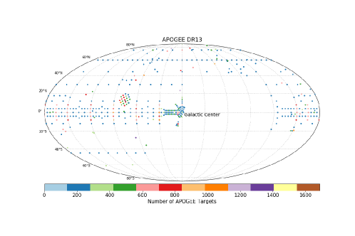
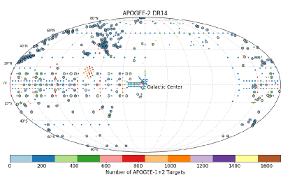
Figures 1 and 2 show the locations of APOGEE data released in DR13 and DR14, respectively. For a more general description of the full SDSS DR13, see SDSS Collaboration et al. (2016), and for DR14, see Abolfathi et al. (2017).

In this paper, we describe the APOGEE DR13 and DR14 data, focusing on changes that were made since the DR12 release (as reported in Holtzman et al. 2015). These include revisions to the APOGEE data reduction pipeline (§3), the APOGEE stellar parameters and abundances pipeline (ASPCAP, §4), the calibrations (§6), and the data that are released (§9). We also assess the modifications made to reduce the impact of persistence (§7) and describe and analyze the results from The Cannon (§8). In addition, we also discuss a few known issues with both DR13 and DR14 that were discovered after the data releases were frozen and made public.

A companion paper (Jönsson et al., 2018) presents assessments of the quality of the DR13 and DR14 stellar parameters and abundances by comparison with independent measurements made from optical spectra of a subsample of APOGEE targets.

Figure 1: Location of fields released in DR13. Different colors represent the number of target stars in different fields.

Figure 2: Location of fields released in DR14. Different colors represent the number of target stars in different fields.

2 The APOGEE spectrograph

All of the data released in DR13 and DR14 were taken with the APOGEE instrument (Wilson et al., 2018) at the Apache Point Observatory (APO), mostly with the SDSS 2.5m telescope (Gunn et al., 2006), but with a few observations taken with an APOGEE instrument feed from the NMSU 1.0m telescope.

As a brief review, the APOGEE instrument is a fiber-fed spectrograph, recording spectra from 300 individual objects in the near-IR (1.51$\mu$m-1.7$\mu$m) at a resolution of $R\sim 22,500$. The spectra are imaged onto three Hawaii-2RG detectors, where each detector records spectra of all 300 objects over roughly a third of the wavelength range, with small wavelength gaps between detectors.

The APOGEE spectrograph at APO was very stable over the course of the SDSS-III survey: it was kept under vacuum and cold continuously for the entire period of operation. During the summer of 2014, the instrument was opened for routine maintenance and to replace one of the three detectors (the so-called “blue” detector that records the shortest wavelength end of the APOGEE spectra). This detector was replaced because it exhibited significant “superpersistence,” as discussed by Nidever et al. (2015). We note that the “green” detector also exhibits some of the same phenomenon at a lower level, but it was not replaced, since we did not have access to an additional detector. The new “blue” detector is of the same Hawaii-2 format as the old one, and therefore it was a simple detector swap with no other associated changes required.

Subsequent to the instrument maintenance, it was pumped and cooled, after which it was refocused. The instrument remained stable under vacuum and cold from then until the summer of 2017.

3 Revisions to the data reduction

The APOGEE data reduction pipeline is described in detail in Nidever et al. (2015). A few modifications in the DR13 and DR14 processing have been implemented as compared with DR12. Changes include an attempt to make some correction for the persistence that occurs over a portion of the APOGEE detectors, improvements in the LSF characterization, a small change in the sky subtraction, improvements in telluric correction, and modified handling of pixels affected by persistence during the construction of the final combined stellar spectra. Details are given in the following subsections.

3.1 Persistence correction

As discussed by Nidever et al. (2015), one of the three original APOGEE detectors (the short wavelength, or “blue” detector) suffers from significant persistence over about a third of its area, and a second detector (the middle wavelength, or “green” detector) shows persistence at a lower level around its periphery. Persistence manifests itself as elevated counts whose amplitude is related to previous exposure on the affected pixels. In DR12, no attempt was made to mitigate the effects of persistence, but data affected by persistence were flagged. Holtzman et al. (2015) present a discussion suggesting that persistence may not impact the derivation of stellar parameters too severely, but does impact the derivation of stellar abundances.

For DR13 and DR14, several modifications were made in an attempt to improve the data with regard to persistence. At the individual exposure level, we implemented a correction to subtract persistence resulting from previous exposures. Significant effort was put into parameterizing the amplitude of the persistence as a function of the previous exposure history. It was found that this is a complex function that depends not only on the previous exposure level and elapsed time, but also on the brightness of the previous source. A complete characterization proved difficult to obtain with extant data, but a first order correction was derived that depends only on the previous exposure level and elapsed time. Specifically, based on an analysis of illuminated frames followed by a series of long dark frames, a double-exponential fit for the amplitude of the persistence was derived for all pixels.

For each science frame, this model was used, along with all of the previous exposures on a given night, to predict the amplitude of persistence in each frame. For most of the science frames, the sequence of science exposures is preceded by two short dark frames (apart from the first plate of the night). The persistence model was also calculated for these frames, and a correction factor was derived to make the predicted persistence better match the observed persistence in these dark frames. This correction factor was then applied to the predicted persistence for the subsequent science frames, in an effort to achieve a more reliable correction. This model was used to try to subtract persistence in both the “blue” and “green” chips.

Subsequent to the production of the DR13 files, we determined that the persistence corrections had been calculated without subtracting the true dark current first. This is not an issue for the “blue” array since it has relatively low dark current, but there are a few regions on the “green” array that have significant dark current and, as a result, the persistence correction resulted in an oversubtraction in these regions. As a result, we disabled the persistence correction for the “green” chip in DR14.

Another, probably more important, persistence amelioration at the visit combination level is discussed below (Section 3.5.2). An evaluation of the effectiveness of these improvements on stellar parameter and abundance determination is presented in Section 7.

3.2 The line spread function

The point-spread function of the APOGEE instrument depends on the location in the spectrograph focal plane, leading to both wavelength and slit/fiber dependence of the line-spread function (LSF). The LSF enters the APOGEE analysis in two ways:

• A fiber-dependent LSF is convolved with an atmospheric model to correct the observed spectra for the effects of telluric absorption.

• The large synthetic library (Zamora et al., 2015) used to derive stellar parameters and abundances in ASPCAP (García Pérez et al., 2016) is convolved with an LSF before comparison with the observed spectra.

The fiber-by-fiber LSF is derived from observations of night sky lines.

For DR13 and DR14, several improvements were made with regard to the LSF. First, it was discovered that one of the OH lines being used for LSF determination had not been appropriately identified as a doublet, leading to an incorrect LSF at the long wavelength end of the “blue” chip, which happens to be where there is significant CO₂ telluric absorption. Second, the functional form of the wavelength dependence of the LSF characterization was modified to provide a better LSF in the same wavelength regime.

Modifications related to the LSF in the stellar parameters and abundances pipeline are discussed in section §4.2.3.

3.3 Night sky subtraction

Emission from the night sky is recorded on a set of “sky” fibers. The reduction pipeline attempts a subtraction of the sky emission using the spectra from sky fibers close in position both in the sky and on the detector. Most of this emission is in bright OH emission lines, and these are generally significantly brighter than the underlying spectra of the objects. As a result, we have not invested significant effort in high precision sky subtraction, because even perfect sky subtraction would still result in a spectrum dominated by the Poisson noise of the sky at the wavelengths of bright OH lines. Instead, we do a simple, highly imperfect subtraction, and flag pixels in the regions around significant sky lines.

The imperfect sky subtraction leads to reduced spectra that are not cosmetically appealing, but the regions near bright lines are ignored in the subsequent analysis. Users of the spectra should be aware of the poor regions of the spectra around sky lines, which are flagged in the data mask that accompanies the spectra.

For DR14, we made one small modification to the sky subtraction, namely we reject spectra from sky fibers that are adjacent to spectra of very bright stars on the detector, since these have the possibility of having inaccurate measurements of any sky continuum. This happens only rarely because our fiber management scheme is designed to avoid it, but there are a handful of observations in which it still occurs.

3.4 Telluric correction

In addition to the improvements in the LSF, a few minor additional modifications were made to the telluric correction routines. These include masking of the regions affected by hydrogen absorption when determining the telluric correction factors, and small modifications in the handling of outliers in the derived correction factors.

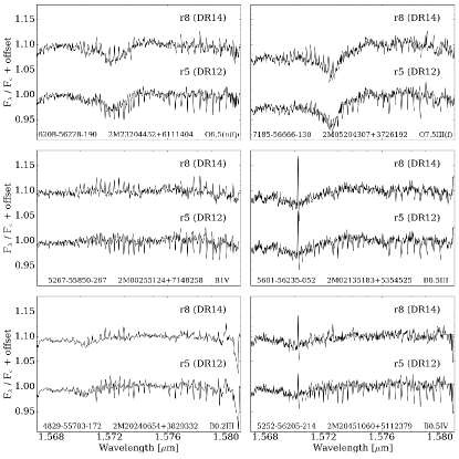
The LSF modifications (§3.2) had the largest impact on the quality of the telluric corrections, and the improvements from these can clearly be seen in essentially all of the hot star spectra and in the quality of the fits to the cooler star spectra. Figure 3 show some example spectra of hot stars that should have nearly featureless continua, in a region of the spectrum with significant CO₂ absorption. Spectra from both DR12 and DR14 are shown that demonstrate, for the most part, significant improvement in the telluric absorption correction with the modifications that were implemented.

Figure 3: A demonstration of the improvement in removal of telluric absorption, comparing DR12 and DR14 visit spectra for a sample of bright OB telluric standard stars. This section of the APOGEE spectra is the most problematic section in terms of telluric features, due to CO₂ telluric absorption. The stellar absorption features visible in some of the spectra are a hydrogen Brackett series line at 1.5704 $\mu$m and a He ii line at 1.5723 $\mu$m.

3.5 Spectra combination

The majority of APOGEE observations consist of multiple visits so radial velocity (RV) variables can be identified while accumulating signal. All of the visit spectra (apVisit files), after shifting to zero RV, are combined into a single final spectrum (apStar files) before the ASPCAP analysis is performed.

3.5.1 Radial velocities

The combination of spectra from multiple visits requires a measurement of the observed velocity shift in each visit, which includes a component from the barycentric correction as well as any RV variation in the object. In DR12 and DR13, the relative RVs were determined iteratively by cross-correlating each visit against the combined spectrum, in an effort to avoid any effects of template mismatch. Once the relative RVs are determined, the final combined spectrum is cross-correlated against a grid of model template spectra to determine the absolute RV.

For DR14, several modifications were made to this scheme. First, in the iterative stage, RVs were determined both by cross-correlation against the summed observed spectra (as before) and also by cross-correlation against a best matching template. The final set of RVs are chosen to be those from whichever of these two methods provides a better result, as quantified by the scatter in the derived individual visit RVs.

In addition, instead of cross-correlating against a full grid of template spectra, the template grid is restricted to include only models with effective temperatures within 750 K of the effective temperature implied by the observed $J-K$ color, using the photometric color-temperature relation of González Hernández & Bonifacio (2009). This was implemented to prevent the choice of an inappropriate template, allowing for some uncertainty in the observed color and extinction, as well as uncertainties in the color-temperature relation.

The modification to the RV determination resulted in slight improvement in the precision of the RVs, as judged by the scatter in the individual visit RVs. As discussed in Nidever et al. (2015), the precision is a function of $T_{\rm eff}$, $\log{g}$, [M/H], and S/N, with a typical value of 100 m/s.

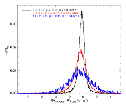
Nidever et al. (2015) suggest an accuracy of $\sim$ 0.35 km/s from APOGEE DR12 based on a comparison of the RVs for 41 stars with literature values. In Figure 4, we compare the APOGEE RVs for over 92,000 stars with RVs from the recent GAIA DR2 (Katz et al. 2018). We find small median offsets between the APOGEE RVs and the GAIA RVs that appear to be a function of mag- nitude, ranging from 0.18 km/s for stars with $6<H<9$ to 0.44 km/s for stars with $11<H<14$. We note that the GAIA RVs are expected to have lower precision than the APOGEE RVs, with precision between 0.2 and 2 km/s, depending on the brightness, $T_{\rm eff}$, etc., of the stars, but that the scatter in the comparison is a bit larger than expected from the combination of the GAIA and APOGEE RV uncertainties. Katz et al. (2018) dis- cuss comparison between the GAIA DR2 RVs and sev- eral catalogs (including APOGEE) and find that other surveys show comparable offsets, but with different de- tails, e.g., as a function of magnitude, making it hard to know what is the correct absolute RV scale at the level of a few hundred m/s.

Figure 4: Comparison of APOGEE DR14 RVs with those from GAIA DR2. Stars are binned in three ranges of H- band magnitude. The scatter is expected to be dominated by uncertainties in the GAIA RVs, but is a bit larger than expected from the GAIA uncertainty estimates.

3.5.2 Weighting of individual visits

For DR13 and DR14, the combination of the spectra was modified in an attempt to reduce the impact of persistence on the derived stellar parameters and abundances, recognizing that the persistence correction (discussed above) is imperfect. Pixels affected by persistence are given reduced weight in the spectral combination process, with several consequences:

• For stars in which only some visit spectra were recorded in the regions affected by persistence, the final resulting spectra are dominated by the unaffected visits, with somewhat larger uncertainties than would have been achieved by weighting all visits equally; the improvement in systematic uncertainties resulting from persistence was judged to be worth the increase in random uncertainties.

• For stars in which all of the visit spectra were recorded in regions affected by persistence, the uncertainty in the pixels/wavelengths affected by persistence are significantly inflated. This has the effect of downweighting them in the ASPCAP fits relative to pixels/wavelengths that are not affected by persistence. Since the S/N that characterizes the combined spectra is the median S/N of all of the pixels, the standard S/N reported for these stars is reduced. To provide a better S/N estimate, we have also calculated an alternate S/N, SNREV, that is determined over a wavelength region in the middle chip that should not have many pixels that can be affected by persistence. SNREV is the recommended quantity to use for S/N assessment.

An analysis of the effect of the modifications in our treatment of persistence is presented in Section 7, and suggests that the modifications resulted in significant improvements.

Another change to the weights in the star combination was made to reduce the impact and inflate the uncertainties of areas of the spectrum affected by sky lines. Regions of individual visit spectra in the vicinity of sky lines were reduced in weight by a factor of 100 in the combination. Unfortunately, there was an implementation error in this for DR13: pixels flagged with PERSIST_LOW were downweighted instead of the SIG_SKYLINE-flagged pixels. This was corrected in DR14.

4 Improvements to the ASPCAP pipeline

The ASPCAP pipeline automatically derives stellar parameters and chemical abundances for the stars observed by APOGEE. The pipeline is described in García Pérez et al. (2016) and Holtzman et al. (2015). In summary, ASPCAP determines the best matching syntheses to the observed spectra, interpolating in previously computed libraries of synthetic spectra (Zamora et al., 2015). A multi-dimensional fit is first done over the entire spectrum to derive stellar parameters, and these parameters are then adopted to do single-parameter fits over limited windows to derive abundances for individual elements.

When we fit for the stellar parameters, we include a [M/H] and an [$\alpha$/M] dimension, plus a [C/M] and [N/M] dimension for giants. As a result, an impact of abundances on stellar parameters only occurs to the extent to which individual elements depart from the abundance ratios in the grid (i.e., deviations from solar abundance ratios in non-$\alpha$ elements, and deviations from [$\alpha$/M] for $\alpha$-elements). When these deviations are small, as they are for most stars, there is not a large effect on stellar parameters. In the cases where there are very atypical abundance ratios, e.g., for second generation stars in globular clusters, we can erroneous stellar parameters, but this is a small fraction of stars.

4.1 Linelist

Several changes were made to the line list adopted for DR12; for details on the construction of the DR12 line list, see Shetrone et al. (2015). New lines were added from NIST and other literature publications, including hyperfine splitting components for Al and Co.

As the synthetic grids were extended to cooler temperatures (see below), lines from H₂O  were added to the line list using the energy levels from Barber et al. (2006). The APOGEE wavelength interval contains more than 26 million H₂O lines and this large number of lines makes computation of the entire spectral libraries with these lines prohibitively expensive in computing time. Tests were carried out that found that H₂O did not contribute significant absorption ($\lesssim$1%) for $T_{\rm eff}$$\geq$4000K, so H₂O lines were not included at these higher effective temperatures. In the cooler library spectra, the H₂O line list was pared down to a computationally manageable number by including a subset of the strongest lines. Tests were done with various cuts in the line strengths, as defined by log (gf$\lambda$) - $\theta$$\chi$_lo (where $\theta$=5040/T and $\chi$_lo=lower excitation potential). Synthetic spectra were computed using increasingly smaller numbers of lines until changes between the complete and reduced line lists produced differences of less than $\sim$1% in flux. After this procedure, we ended up using a list containing 443448 lines for for 3250$<$$T_{\rm eff}$$<$4000K or [M/H]+[$\alpha$/M]$<$-1.5, and a list with 1891110 lines for $T_{\rm eff}$$<$ 3250 and [M/H]+[$\alpha$/M]$>$-1.5.

Astrophysical gf values for the atomic lines were derived adopting the same methodology as for DR12 (Shetrone et al., 2015). One change implemented for DR13/14 was the use of the synthesis code Turbospectrum (Alvarez & Plez 1998, Plez 2012) to generate synthetic spectra with varying oscillator strengths and damping values to fit the solar and Arcturus spectra, respectively. The use of Turbospectrum provides consistency with the calculation of the synthetic libraries described below. For DR12 the code MOOG (Sneden 1974) was used, while the computation of the spectral libraries was done using ASS$\epsilon$T (Koesterke, 2009).

When deriving astrophysical $\log gf$ values, the DR13/DR14 line list used a different weighting scheme to combine the results from the Sun and Arcturus than that described in Shetrone et al. (2015): the astrophysical solutions were weighted according to line depth in Arcturus and in the Sun, which usually gives more weight to the Arcturus solution since the lines are generally stronger in the cooler, low surface gravity star, Arcturus, despite it being more metal-poor. When comparing with the center-of-disk solar spectra, a center-of-disk spectral synthesis with a microturbulence of 0.7 km s^-1 was used (correcting a previous error for the DR12 line list where a full-disk synthesis was used).

The adopted abundances for Arcturus were also updated and modified slightly, based on new, careful comparisons with the literature, while retaining the Asplund et al. (2005) abundances for the Sun. For the DR12 line list, Arcturus abundances of [$\alpha$/Fe]=0.4 for the $\alpha$ elements, [Ca/Fe]=0.1, [Al/Fe]=0.3, and [X/Fe]=0. for all others were adopted, assuming values typical of thick disk stars, but with Al and Ca adjusted based on measurements by Ramírez & Allende Prieto (2011). For DR13/14, we adopted the abundances from Ramírez & Allende Prieto (2011) exactly. For the underlying atmospheric model used to do the Arcturus synthesis, a model with [X/H]=-0.50 and [$\alpha$/Fe]=0.25 was adopted, i.e. roughly, but not exactly, consistent with the abundances used in the synthesis. The adopted stellar parameters and abundances for Arcturus for both the model atmosphere and synthesis are given in Table 1; we include for reference the values adopted for the DR12 synthesis.

Table 1: Adopted Arcturus parameters/abundances

Quantity	DR13/14 model	DR12	DR13/DR14
	atmosphere	synthesis	synthesis
Teff	4286	4286	4286
$\log{g}$	1.66	1.66	1.66
[M/H]	-0.50	-0.52	-0.52
C	7.89	7.96	7.96
N	7.28	7.64	7.66
O	8.41	8.64	8.62
Na	5.67	5.65	5.86
Mg	7.28	7.41	7.38
Al	5.87	6.15	6.25
Si	7.26	7.39	7.32
P	4.86	4.84	4.91
S	6.89	7.02	6.97
K	4.58	4.80	4.76
Ca	6.06	5.89	5.88
Sc	2.55	2.53	2.72
Ti	4.65	4.78	4.63
V	3.50	3.48	3.64
Cr	5.14	5.12	5.07
Mn	4.89	4.87	4.75
Fe	6.95	6.93	6.93
Co	4.42	4.40	4.44
Ni	5.73	5.71	5.74
Cu	3.71	3.69	3.64

4.2 Synthetic spectral grids

The ASPCAP pipeline determines stellar parameters and abundances by finding the best match between observed spectra and a large grid of synthetic spectra, using the FERRE code (Allende Prieto et al., 2006) to determine the best match. The synthetic spectral grid is multi-dimensional, since the main features in the near-IR portion of the spectra can depend on multiple quantities, including $T_{\rm eff}$, $\log{g}$, [M/H], [$\alpha$/M], [C/M], [N/M], microturbulent velocity, macroturbulent velocity, and stellar rotation.

Several modifications were made for the spectral grids used in DR13 and DR14, and these are discussed below.

4.2.1 Inclusion of a cool grid

For DR12, we used grids covering two temperature ranges: the GK grid (3500-6000 K), and the F grid (5500-8000K). For DR13/DR14, we added cooler (M) grids for giants and dwarfs. However, we could not compute the M grids using Kurucz model atmospheres as we did for the warmer grids, since Kurucz atmospheres are not available below 3500 K. In addition, very cool giants are expected to have large radii where sphericity effects are likely to be important. As a result, we used a set of self-consistent MARCS model atmospheres (Gustafsson et al., 2008) computed specifically for the APOGEE project by B. Edvarsson for the M grid. While it would be preferable to use a homogeneous set of model atmospheres in all calculations, Kurucz atmospheres are not available at cooler temperatures, and MARCS atmospheres were only available in a coarser grid at warmer temperatures. For subsequent data releases, we are planning on using a homogeneous grid, with a spacing in stellar parameters similar to the Kurucz grid, based on a new grid of MARCS model atmospheres.

The M grid of model atmospheres covers the range between 2500-4000 K in steps of 100K, $\log{g}$  from -0.5 to 5 in steps of 0.5, [M/H] from -2.5 to 0.5 in steps of 0.5 dex, and [$\alpha$/M] and [C/M] from -1.0 to 1.0 in steps of 0.5 dex. Unfortunately, a significant fraction ($\sim$ 20%) of the model atmospheric structures could not be computed because of convergence issues; while many of these failures were on a grid edge in one or more dimensions, there are some that fall within the grid. To complete the rectangular grid needed for the FERRE analysis, we filled in the missing models with the “nearest” adjacent models, where the following metric was adopted:

$$dist=0.7|\Delta\textrm{[M/H]}|+0.4X|\Delta\textrm{[$\alpha$/M]}|+\\ 0.17X|\Delta\textrm{[C/M]}|+0.62|\Delta\textrm{$T_{\rm eff}$}|/100.+\\ 1.5|\Delta\textrm{$\log{g}$}|$$ (1)

where $X$ was taken to be unity for models where [C/M]-[$\alpha$/M] had the same sign as [C/M]-[$\alpha$/M] of the missing model, and $X=4$ for those where [C/M]-[$\alpha$/M] had an opposite sign. This prescription was developed in an effort to choose those neighboring model atmospheres that are expected to be most similar to the missing ones: a change in [C/M] is probably less significant than a change in [$\alpha$/M], which is less significant than a change in $T_{\rm eff}$, etc. After adopting the nearest model atmosphere, the appropriate abundances for the grid location were used in the synthesis.

In practice, the presence of the missing models is most significant for the coolest giants and for cooler dwarfs. Figure 5 shows the location in an HR diagram of stars in DR14 for which there is a missing model within one grid point in any of the dimensions in the relevant grids. More locations are affected that have a missing model within two grid points, i.e., are still relevant for the cubic interpolation that is used.

Figure 5: Location in an HR diagram of DR14 stars that have parameters within one grid point (ATMOS_HOLE_BAD bit set) of the best fit solution in any of the dimensions of the fit. Color indicates the overall metallicity of the stars.

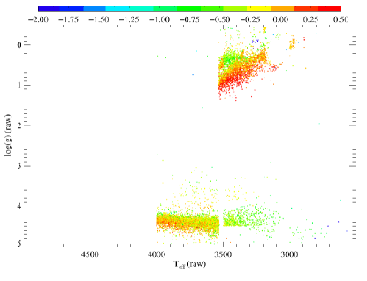
While DR13 and DR14 do include results from the M grid, there are a number of issues that warrant caution in the use of resulting parameters and chemical abundances for M dwarfs and giants:

• The MARCS grids are coarser than the Kurucz grids, with a spacing of 0.5 in [M/H], [$\alpha$/M], as opposed to 0.25 for the Kurucz grids.

• Inaccuracies may occur because of the missing models that have been filled as described above. This is especially severe given the coarseness of the MARCS grid, which results in only five points in the [$\alpha$/M] and [C/M] dimensions, since the cubic interpolation used by FERRE considers four points in each dimension of the grid. For DR14, we implemented a flag to warn when the interpolation includes a point for which a neighboring model atmosphere was used in the solution for a given star.

• In the transition region between the cool and warm grids ($T_{\rm eff}$$\sim$ 3500 K) for giants, there are significant discontinuities in the sets of results from the Kurucz and MARCS models (see 5). Some discontinuity is expected because of the different geometries of the two sets of models.

4.2.2 Spectral synthesis

For DR13/DR14, we adopted the publicly available Turbospectrum code (Plez, 2012), rather than the ASS$\epsilon$T (Koesterke, 2009) synthesis code that was used for DR12 and previous versions. On top of the self-consistency mentioned in §4.1, an additional motivation for this change included the public availability and the related ability to run the synthesis on the SDSS computer cluster with different input parameters, reducing the need for transfer of large data sets.

For previous releases, a single set of grids, covering different temperature ranges, were used to get parameters and abundances for both giants and dwarfs. For DR13, we have split the grids to allow giants and dwarfs to be treated differently, in several respects:

• For the giant grids, we adopt carbon isotopic ratios more appropriate for low surface gravity stars (${}^{12}C/^{13}C=15$); for the dwarf grids, we use solar isotopic ratios (${}^{12}C/^{13}C=90$). For DR12, solar isotopic ratios were used for all grids.

• For the dwarf grids, we allowed for the non-negligible stellar rotation that is observed in a substantial fraction of dwarfs; previous data releases only used grids without rotation. To allow for the storage required by this extra dimension, we eliminated the [C/M] and [N/M] dimensions and set [C/M]$=$[N/M]$=0$ at the parameter fitting stage (but see below); the need for these dimensions in dwarfs is reduced because the mixing that leads to significant variations in [C/M] and [N/M] in giants is not present in dwarfs.

Spectra were calculated at a fixed wavelength spacing of 0.05 Å, but were subsequently resampled (after LSF convolution) to a uniform spacing in $\log\lambda$, with $d\log\lambda=6.e-6$ (corresponding to 1.8 km/s/pixel), and split into three sections corresponding to the wavelengths covered by the three APOGEE detectors. For the DR13/DR14 libraries, we also expanded the wavelength range stored for each detector slightly compared with the DR12 libraries, to allow for the inclusion of a few additional lines. However, data for all stars may not be available in the expanded region because of different radial velocity shifts. To ensure that the same wavelengths are used for the determination of stellar parameters in all stars, the trimmed wavelength range that was used for the DR12 libraries was adopted in the global parameter fit via an input mask, and the extended spectra were only used for the fits for individual element abundances. Table 2 gives the wavelength ranges that were used.

Table 2: Wavelengths stored for synthetic grids

Detector	$\log\lambda_{0}$	npixels	d$\log\lambda$	wavelength range
DR12
blue	4.180932	2920	6.e-6	15168.13 - 15792.32
green	4.200888	2400	6.e-6	15881.37 - 16416.55
red	4.217472	1894	6.e-6	16499.55 - 16936.75
DR13/DR14
blue	4.180476	3028	6.e-6	15152.21 - 15799.31
green	4.200510	2495	6.e-6	15867.55 - 16423.81
red	4.217064	1991	6.e-6	16484.05 - 16943.53

4.2.3 Separate grids for different LSFs

Subsequent to DR12, we recognized that the variable LSF across the detector results in small systematic differences in stellar parameters and abundances depending on where spectra were recorded on the instrument detectors, when analyzed using a single synthetic grid calculated with an average LSF (see also Ness et al. 2017).

To partially account for the fact that the LSF varies with location on the detector, for DR13/DR14 we constructed and used five different versions of each grid, one for an average LSF, and four others for four different fiber ranges that capture the main variations of the LSF with fiber. We determined the different fiber ranges using a clustering analysis of the LSF’s FWHM at three representative wavelengths: $15450\,\AA$, $16130\,\AA$, and $16740\,\AA$ in the blue, green, and red detectors, respectively. We clustered the FWHMs at these three wavelengths using a Gaussian mixture (using the XD code; Bovy et al. 2011) and we determined with a cross-validation test set of 60 fibers that four fiber groupings suffices to capture the variation of the LSF with fiber at these wavelengths. These fiber ranges are: 1-38, 39-150, 151-250, 251-300. Within each of these, LSFs from five fibers were averaged and used to create each spectral grid.

While this change in LSF strategy should be an improvement over the single average LSF used for the DR12 grids, it is still an approximation because:

• The LSF varies continuously, even within the adopted ranges.

• Most stars are obtained on multiple visits where different fibers are used in different visits. Generally, the fibers from different visits lie relatively near one another on the slit, but this is not always the case; we adopt the LSF grid appropriate to the mean fiber position of the fibers in which observations were obtained. However, the typical dispersion in FWHM of a single star over different visits is only $\approx$ 20% of the full dispersion of FWHM over all 300 fibers.

4.2.4 Spectral synthesis grid management

Because of the separation of giant/dwarf grids, the addition of the cool grids, and the multiple LSF grids, the DR13 and DR14 analyses involves a large number of grids: F dwarf, GK dwarf and giant, and M dwarf and giant, with five different LSFs for each, leading to 25 total grids. To avoid having to run FERRE on all stars through all of the temperature grids, we perform initial coarse characterization fits with the F dwarf grid, the GK giant grid, and the M giant grid. In these fits, [C/M] and [N/M] are set to solar, and an average LSF is used for all stars. Based on the derived $T_{\rm eff}$ and $\log{g}$ from this coarse characterization, full fits are done in the different grids according to:

• stars with $T_{\rm eff}$$>$ 5000K are fit with the F grid

• stars with 3000 $<$ $T_{\rm eff}$$<$ 6000K and $\log{g}$$<$ 4 are fit with the GK giant grid

• stars with 3000 $<$ $T_{\rm eff}$$<$ 6000K and $\log{g}$$>$ 3.5 are fit with the GK dwarf grid

• stars with $T_{\rm eff}$$<$ 4000K and $\log{g}$$<$ 4 are fit with the M giant grid

• stars with $T_{\rm eff}$$<$ 4000K and $\log{g}$$>$ 3.5 are fit with the M dwarf grid

For stars that are fit with multiple grids (note that there is overlap in the ranges), we adopt the fit with the lowest $\chi^{2}$. We avoid mixing MARCS and Kururcz results above 3500K by severely penalizing the MARCS grid above 3500K (by increasing the $\chi^{2}$ by a factor of ten). We also penalize fits within 1/8 of a grid step of any grid edge (by increasing $\chi^{2}$ by 25%). The parameters from the adopted fit are used to derive the stellar abundances.

As described in §9, we record and release information on which was the best grid for each star, and also release the parameters from all grids that were used for a given star.

4.3 Pseudo-continuum normalization

Before the observed spectra can be compared with model spectra, they must be continuum-normalized to remove instrument/reduction signatures (e.g., fiber-dependent and wavelength-dependent sensitivities) and continuum slope introduced by interstellar absorption. To ensure a correct comparison, both observed and model spectra are normalized in the same way. In DR13 and prior data releases, a polynomial fit with an iterative asymmetric rejection scheme (preferentially rejecting low pixels to high pixels) was used to do this normalization, in an effort for the normalization continuum to more closely approximate the true continuum, i.e. by rejecting absorption lines in the continuum fit.

However, the asymmetric rejection causes the derived continuum to be a function of S/N, especially at lower S/N, because pixels with larger statistical fluctuations that are below the continuum are rejected in the fit, biasing the fit high. This is apparent, e.g., in metal-poor stars that have weaker absorption features, in which statistical fluctuations in the continuum in lower S/N spectra may be rejected. To remove this bias, DR14 adopts a continuum normalization that is just a straight 4th order polynomial fit to the spectrum, with no iterative rejection. To avoid contamination of the fit from bad pixels, e.g., those with imperfect sky subtraction, pixels marked as bad or in the vicinity of sky lines in the observed spectra are masked in the fit. It is not possible to use the same masks for the model as for the observed spectra because sky features appear at different rest wavelengths in stars with different radial velocities, so no pixels are masked in the fits to the model spectra. Since the fit is low order, however, applying masks to the model spectra would have little effect.

Because of the new normalization scheme, the pseudo-continuum normalized spectra in DR14 have a noticeably different mean level than for spectra in previous data releases; in DR14 pseudo-normalized spectra, there is a significant number of pixels with values above unity.

4.4 Fitting for stellar parameters

The details of the spectral fitting procedure differed slightly between DR13 and DR14, as described in the following subsections. One new feature, discussed below, for both DR13 and DR14, (as compared with DR12) is that a relation for the macroturbulent velocity as a function of other stellar parameters was derived and adopted (e.g., Massarotti et al. 2008); for DR12, a single value was used for all stars.

4.4.1 DR13

For red giants, the best matching spectral syntheses are obtained from fits in 6D ($T_{\rm eff}$, $\log{g}$, [M/H], [$\alpha$/M], [C/M], and [N/M]), adopting relations for microturbulent and macroturbulent velocities that are a function of the other parameters. These relations were derived as follows.

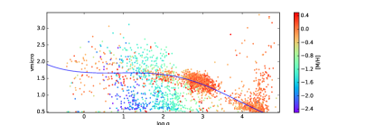
First, a 7D fit ($T_{\rm eff}$, $\log{g}$, microturbulent velocity, [M/H], [$\alpha$/M], [C/M], and [N/M]), adopting a fixed macroturbulent velocity of 4 km/s, was performed on a stellar calibration subsample that was chosen to include stars from across the HR diagram. Figure 6 shows the derived microturbulent velocities as a function of surface gravity, color-coded by metallicity. At lower metallicity, the weaker lines are expected to be less sensitive to microturbulent velocity, perhaps explaining the large scatter seen in these stars. From these results, a cubic fit to surface gravity was derived using stars with [M/H]$>-1$ and $\log{g}$$<3.8$, giving the following relation:

$$v_{micro}=10.^{\left(0.226-0.0228\log g+0.0297(\log g)^{2}-0.0113(\log g)^{3}\right)}$$ (2)

Figure 6 shows this adopted fit.

Figure 6: Derived microturbulent velocity as a function of surface gravity for DR13 calibration sample (points), and adopted relation for microturbulent velocity (line). Color of the points indicate the metallicities of the stars.

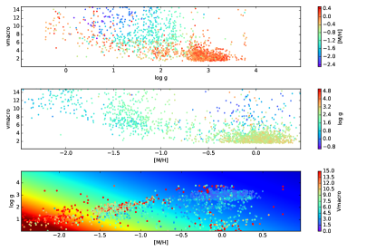
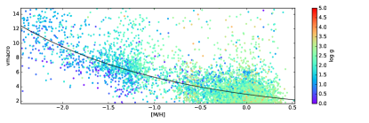
Adopting this relation, we perform another 7D fit, now adding macroturbulent velocity as a free parameter. Figure 7 shows derived macroturbulent velocity as a function of both [M/H]and $\log{g}$. Based on these, we adopted a 2-D fit depending on both quantities:

$$v_{macro}=10.^{\left(0.741-0.0998\log g-0.225[M/H]\right)}$$ (3)

Figure 7 shows the derived macrotubulent velocities and the adopted fit. Since the derived relation is a strong function of metallicity, we cap the maximum macroturbulent velocity at 15 km/s, to avoid extrapolation.

Figure 7: Derived macroturbulent velocity for DR13 calibration sample. Top panel shows $v_{T}$ as a function of surface gravity, middle panel as a function of metallicity, and bottom panel shows adopted 2D fit. Colors of the points encode the metallicity, surface gravity, and macroturbulent velocity, respectively, as indicated by the color bars.

Finally, a 6D grid is generated, adopting the relations for both microturbulent and macroturbulent velocities, and this grid is used to derive stellar parameters and abundances for the entire sample.

For dwarfs, an additional dimension to account for stellar rotation is needed, so the same methodology would require a 7D grid. The effects of stellar rotation and macroturbulence are essentially indistinguishable at the spectral resolution of the APOGEE spectra. To reduce the dimensionality of the fit, we take advantage of the fact that dwarfs do not show the same range of [C/M] and [N/M] variations as is seen in red giants. As a result, we derived stellar parameters setting [C/M]$=$[N/M]$=0$ and using a 6D grid ($T_{\rm eff}$, $\log{g}$, microturbulent velocity, [M/H], [$\alpha$/M], and $v\sin i$) for dwarfs. However, this choice leads to significant problems in the derivation of C and N abundances in dwarfs, as discussed below.

4.4.2 DR14

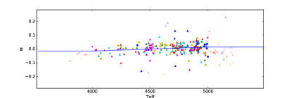
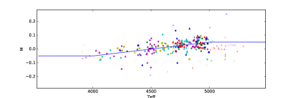
For DR14, a similar scheme was adopted, with one significant change for giants: microturbulent velocity was left as a free parameter in the final fits, i.e., 7D fits in $T_{\rm eff}$, $\log{g}$, microturbulent velocity, [M/H], [$\alpha$/M], [C/M], and [N/M] were done. While this increased the computational analysis time significantly (by roughly a factor of five), it was felt to be warranted for two reasons. First, from the initial calibration sample fit, there was a non-negligible range in derived microturbulent velocity in some regions of $T_{\rm eff}$-$\log{g}$-[M/H] parameter space. Second, the derived metallicities of cluster stars showed less of a trend with effective temperature when the microturbulent velocity was allowed to float as a free parameter than when a fixed relation was adopted; see Figure 8.

Figure 8: Derived raw [M/H] vs $T_{\rm eff}$ for stars in clusters, allowing for microturbulent velocity to float (upper) vs fixing with a relation based on $\log{g}$  (bottom). There is significantly less trend with temperature when microturbulent velocity is left as a free parameter. Different point colors and symbols are used to distinguish different clusters.

Although the basic methodology was the same as for DR13, DR14 adopted a different prescription for macroturbulent velocity, with a dependence only on metallicity (see Figure 9):

$$v_{macro}=10.^{\left(0.471-0.254[M/H]\right)}$$ (4)

Figure 9: Derived macroturbulent velocity relation as a function of [M/H] for DR14 calibration sample; point color encodes the surface gravity, as indicated by the color bar. Line shows the adopted relation.

For dwarfs, the DR14 methodology was the same as the DR13 methodology.

4.5 Fitting for stellar abundances

After the stellar atmospheric parameters are determined for each star, individual elemental abundances are determined using spectral windows located on features of each element, varying the [M/H], [$\alpha$/M], [C/M], or [N/M] dimension of the grid, depending on the element, with other dimensions fixed, i.e., the [$\alpha$/M]  dimension is used to derive abundances for the different $\alpha$-elements (O, Mg, Si, S, Ca, Ti) and the [M/H]  dimension is used for all other elements (except C and N in giants, see below). We note that, as in previous releases, the stellar parameter dimensions are fixed to their fitted values, i.e., before any calibrations (discussed below) are applied. The rationale for this is that these values provide the best match of synthetic spectrum, hence would do the best job in removing blends from lines of interest. In addition, differences between the uncalibrated spectroscopic parameters and independent estimates may be absorbing inaccuracies in some of the assumptions in the models, such as the 1D LTE methodology.

Carbon and nitrogen abundances in giants were determined by varying the C and N dimensions in the grid, which provides an accurate modeling of their abundances. However, as discussed above, the grids for dwarfs do not have separate C and N dimensions. As a result the metallicity dimension was used to solve for C and N in dwarfs. However, it was subsequently realized that this procedure is fundamentally flawed because the C and N abundances come largely from molecular lines. For these lines, the metallicity dimension changes abundances of all constituent species simultaneously, so leads to incorrect results for C and N. So while C and N abundances should be reliable in giants, they are not in dwarfs, and should not be used in the latter.

4.5.1 New elements and revised element windows

DR13/DR14 includes detailed abundances for additional elements that generally have weaker lines than the 15 elements presented in the previous data releases: the newly added elements include P, Co, Cr, Cu, Ge, Rb, Nd (Hasselquist et al., 2016), as well as carbon abundances from atomic lines of C I. We also note that although an abundance labelled Y (yttrium) is provided, the dominant feature in the windows used for this is actually a Yb (ytterbium) line, so no meaningful abundance is provided. As discussed below, the lines from many of these elements are weak and sensitive to blending, and abundances from them should be used with caution, if at all. The current methodology does not produce meaningful results for elements that are derived from a feature that is blended with a line from another element that varies in the same dimension in the grid; we are considering how best to ameliorate this for future analysis.

The procedure used to determine the windows for each element was slightly modified from that used for DR12. The windows were determined by finding regions of the spectrum that are sensitive to variations in the abundance of each element (at the stellar parameters of Arcturus), while at the same time being less sensitive to the variation of other elements within the same grid dimension, and weighting pixels according to these considerations. Within these windows, higher weight was given to features where a model Arcturus spectrum better matches the observed Arcturus spectrum.

The window determination also uses the mean residuals from fits to the full APOGEE sample. In DR12, those pixels with residuals larger than a given threshold were removed by assigning them zero weight. This results in some windows with peculiar shapes; the windows for Al provide a good example. To avoid this, we adopted for DR13/DR14 the same procedure used to identify pixels not well reproduced in the Arcturus spectrum, but instead of simply completely removing those pixels with larger differences, they are scaled from the pixel with the largest residuals, which is assigned a zero value, to the pixels at the threshold, which are not downweighted. Therefore, pixels with residuals near the threshold have weights close to one (i.e., the weights of the pixel are only slightly lowered) and only the pixel with the largest residuals is completely removed.

5 Effect of model atmospheres

As described in section 4.2.1, stellar atmospheres from Kurucz were used for the bulk of the sample, but MARCS stellar atmopheres were used for stars with $T_{\rm eff}$$<$3500 K. However, there was an overlap region between $3500<$$T_{\rm eff}$$<4000$ in which stars were fit by both grids.

Figure 10 shows the uncalibrated spectroscopic HR diagrams in this effective temperature range derived using the Kurucz (left panel) and MARCS (right panel) atmospheres. The transition between the two atmospheres is easily seen at 3500K in the left panel and at 4000 K in the right panel.

Figure 10: Raw spectroscopic HR diagrams at $3500<$$T_{\rm eff}$$<4000$ K derived using Kurucz atmospheres (left) and MARCS atmospheres (right). Point color is used to represent the derived [M/H]. As discussed in the text, results from the Kurucz atmospheres were adopted in this temperature range for DR13 and DR14.

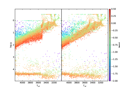
For DR13 and DR14, we have adopted the results from the Kurucz grid in this temperature regime. Several factors contributed to this choice. First, the MARCS grid available at the time was significantly coarser than the Kurucz grid, so this led to a preference for the Kurucz grid, especially for regions in $T_{\rm eff}$ and $\log{g}$ where sphericity effects are not expected to be very significant (i.e., warmer than 4000-4500 K). Given this choice, we felt that it was better to use a homogeneous grid extending to 3500 K rather than to mix results from different sets of atmospheres. On top of this, results from the Kurucz grid seem to show a cleaner trend of stellar parameters with metallicity at $3500<$$T_{\rm eff}$$<4000$ K on the upper giant branch than the results from the MARCS grid (seen as the mix of colors in the upper giant branch in the right panel of Figure 10).

Clearly, this leaves a significant discontinuity at 3500 K, which leads to our recommendation that results below 3500 K be used with extreme caution, and recognition of the fact that there may be systematic uncertainties for stars with $3500<$$T_{\rm eff}$$<4000$ K.

Subsequent to this analysis, a finer grid of MARCS models has been calculated by one of us (BE), which should allow a homogeneous analysis over the full effective temperature range, so future data releases will likely use these atmospheres.

6 Calibrations and uncertainties

In this section, we describe the calibrations that have been derived for the values of stellar parameters and elemental abundances from the spectral fits. We also describe how we derive empirical uncertainties in these quantities. To avoid over-complication and since DR14 supercedes DR13, we present here the DR14 calibrations in detail and only qualitatively describe the DR13 calibrations; additional details on DR13 are presented in an Appendix.

6.1 Effective temperature calibration

In DR12, the spectroscopic temperatures were compared with photometric temperatures from González Hernández & Bonifacio (2009) and a single zero-point correction was applied to provide a “calibrated” effective temperature.

6.1.1 DR13

Subsequent inspection of the different photometric temperature calibrations from the literature highlighted that different photometric scales differ by an amount comparable to the offset applied to DR12. Given the uncertainty in photometric temperature scales, it was decided that no external calibration would be applied to the effective temperatures in DR13.

After the DR13 release was frozen, however, it became apparent that there are trends in the comparison of DR13 spectroscopic temperatures with photometric temperatures, in particular, as a function of metallicity. As a result, we have suggested a “post-calibration” correction to effective temperatures, as described in Appendix A.1.

6.1.2 DR14

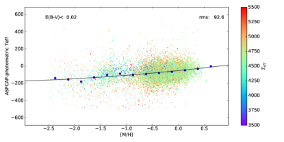
Because of the issues discovered with DR13, a calibration relation for $T_{\rm eff}$  was adopted for DR14. Figure 11 shows the difference between DR14 raw ASPCAP derived effective temperatures and photometric temperatures for a low reddening ($E(B-V)<0.02$) sample. A trend with metallicity exists, but it is not so large as in DR13; the improvement comes from a revised handling of the normalization of the spectrum. It should be kept in mind that the photometric effective temperature scales may also have uncertainties.

We adopted an effective temperature calibration that is a quadratic function of metallicity:

$$T_{eff}(ASPCAP)-T_{eff}(GHB)=A_{Teff}+\\ B_{Teff}[M/H]+C_{Teff}[M/H]^{2}$$ (5)

with separate parameters for giants and dwarfs, as given in Table 3, where we define giants to have:

$$\log g<2./1300(T_{eff}-3500)+2$$ (6)

The adopted calibration relations are shown in Figure 11. These relations were derived from giants with $3750<T_{eff}<5500$ and from dwarfs with $4000<T_{eff}<7500$. They were applied to all stars with $T_{eff}>3532$, pinning the applied correction to the lower and upper ends of the range from which the relations were derived outside of that range.

Table 3: Parameters for DR14 $T_{\rm eff}$ calibration.

Sample	$A_{Teff}$	$B_{Teff}$	$C_{Teff}$
giants	-51.59	61.48	7.176
dwarfs	-36.38	13.16	-26.10

Figure 11: Relation between raw DR14 ASPCAP $T_{\rm eff}$ and photometric $T_{\rm eff}$  from González Hernández & Bonifacio (2009) as a function of metallicity (color-coded by $T_{\rm eff}$) for giants (top) and dwarfs (bottom). Large red and blue points show mean and median difference in bins of metallicity. Curves show derived and adopted DR14 calibration.

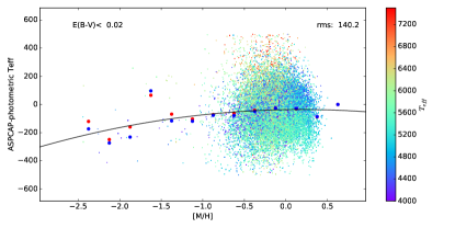
While our relation is derived from a comparison with photometric effective temperatures, we note that Jönsson et al. (2018) provide an independent indication that even the calibrated ASPCAP temperatures have a small remaining metallicity-dependent error with respect to optical spectroscopic $T_{\rm eff}$, highlighting the challenge of achieving a true effective temperature scale.

For an estimate of the uncertainties in $T_{\rm eff}$, we calculate the scatter between the photometric and spectroscopic effective temperatures in bins of $T_{\rm eff}$, [M/H], and S/N, and a linear surface fit was performed to derive coefficients that approximate the observed scatter:

$$\ln(\sigma_{Teff})=A_{\sigma Te}+B_{\sigma Te}(T_{eff}-4500)+\\ C_{\sigma Te}[M/H]+D_{\sigma Te}(S/N-100)$$ (7)

where we fit to the logarithm to ensure that the uncertainty never reaches negative values (i.e., outside of the range of the calibration data). Again, a separate fit was performed for red giants and dwarfs, with parameters as given in Table 4.

Table 4: Parameters for DR14 $T_{\rm eff}$ uncertainties.

Sample	$A_{\sigma Te}$	$B_{\sigma Te}$	$C_{\sigma Te}$	$D_{\sigma Te}$
giants	4.361	0.000604	-0.00196	-0.0659
dwarfs	4.583	0.000290	-0.00130	-0.243

The fit surfaces are shown in Figure 12, which demonstrate that the $T_{\rm eff}$ uncertainties are largely a function of $T_{\rm eff}$, with larger uncertainties at higher temperatures.

Figure 12: Measured scatter in $T_{\rm eff}$ in bins of [M/H], $T_{\rm eff}$, and S/N (different panels): color of points give observed scatter. Background color shows derived fit that was used to determine uncertainties for individual stars.

6.1.3 Raw and calibrated effective temperatures

Both the raw and calibrated temperatures are included in the data release, although, as noted above, the calibrated and uncalibrated effective temperatures are identical in DR13. Raw quantities can be found in the FPARAM array, while calibrated quantities are found in TEFF and in the PARAM array.

6.2 Surface gravities

Spectroscopic surface gravities are challenging to derive accurately. We have taken the approach of calibrating the derived surface gravites using observations of stars in the Kepler field, for which high precision measurements of surface gravity are available from asteroseismic analysis (Pinsonneault et al., 2014); we adopted asteroseismic values from version 3.6.0 of the APOKASC catalog.

For DR12, Holtzman et al. (2015) discuss offsets between the ASPCAP values of $\log{g}$  when compared to those derived from asteroseismology; the differences between asteroseismic and spectroscopic surface gravities was found to be different for red giants and red clump stars. For DR14, the offsets between the ASPCAP and asteroseismic surface gravities have been reduced slightly, which results from the improved treatment of the LSF and macroturbulence. However, differences still remain, including the offset between red giant (RGB) stars and red clump (RC) stars that deserve further study (see, e.g., Masseron & Hawkins 2017).

The surface gravities for dwarf stars are more problematic. The spectroscopic surface gravities for dwarfs generally seem to be too low, especially for cooler stars, based on expectations from stellar isochrones. In addition, we do not have a significant number of asteroseismic calibrator for dwarfs. As a result, we do not provide calibrated surface gravities for dwarf stars at all, and defer improvements on this issue to subsequent analysis.

The following subsections describe the surface gravity calibrations applied to giants for DR13 and DR14.

6.2.1 DR13

For DR13, we adopted a $\log{g}$  correction for red giants that depends both on surface gravity and metallicity. We note that this differs from DR12, where only a surface gravity dependence was found and calibrated. As with DR12, separate corrections were derived for RGB and RC stars. Due to limited availability of asteroseismic data when the calibration was frozen, we chose to clip the metallicity correction to [M/H]$>$-1.5. Subsequent analysis of addditional data demonstrate that this clipping was incorrect, so we recommend a “post-calibration” correction to the DR13 surface gravity for low metallicity stars.

Appendix A.2 provides the details of the DR13 surface gravity calibrations and recommended correction, including the criteria used to distinguish RGB and RC stars.

6.2.2 DR14

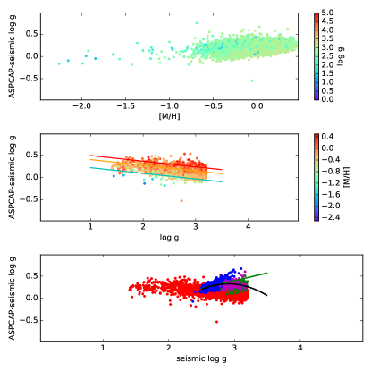
Figure 13 shows the difference between raw DR14 ASPCAP and asteroseismic surface gravities for red giant stars. The top panel of Figure 13 demonstrates a trend with metallicity, the middle panel demonstrates a trend with surface gravity (RGB stars only), and the bottom panels shows the difference between RGB stars (red) and RC stars (blue). From these data, we derived separate calibration relations for RGB and RC stars:

$$\log g=\log g(raw)-(0.528-0.127\log g+\\ 0.183[M/H])$$ (8)

for RGB stars, and, for RC stars:

$$\log g=\log g(raw)-(-0.643+0.346\log g+\\ 0.0147[M/H])$$ (9)

Unfortunately, we discovered after the data release that the RC stars denoted as such in the APOKASC catalog do not include so-called secondary clump stars, which are denoted as 2CL, with transition objects denoted as RC/2CL; these are shown in the bottom panel of Figure 13 as green and magenta points, respectively. As a result, the calibration relation derived and applied for RC stars (green line) is not valid for the RC/2CL and 2CL stars; rather than increasing, the correction should decrease for the higher surface gravity core helium burning stars. We discuss how to do so below.

Figure 13: Comparison of raw ASPCAP surface gravity with asteroseismic surface gravity. Top panel shows difference between spectroscopic and asteroseismic surface gravity as a function of metallicity, color-coded by gravity. Middle panel shows difference as a function of surface gravity, color-coded by metallicity, for red giants only; lines show derived RGB calibration relation for metallicities 0.5, 0, and -1. Bottom panel shows different as a function of surface gravity, with RGB sample in red, RC sample in blue, 2CL sample in green, and 2CL/RC sample in magenta (see text for description); the green line shows the RC calibration relation used for DR14, while the black line show the recommended RC calibration.

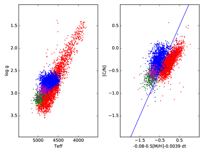
To apply a separate calibration for RGB and RC stars requires some way of distinguishing them for stars without asteroseismic analysis. We revisited the methodology used in DR12 for RC/RGB separation using the asteroseismic sample (which provides an RC/RGB classification from seismology). The basic idea is to use a ridgeline in the $T_{\rm eff}$-$\log{g}$  plane that is a function of metallicity, and supplement this with the measurements of the [C/N] ratio, since this is expected (and observed) to further separate the RGB and RC. We define a difference, $\Delta t$, between ASPCAP $T_{\rm eff}$  and a metallicity-dependent ridgeline:

$$$$\Delta t=T_{eff}(raw)-(4444.14+554.311(\log g(raw)-2.5)-\\ 307.962[M/H](raw))$$$$ (10)

Using these definitions, we then classify stars as RC if $2.38<$$\log{g}$$<3.5$ and

$$\textrm{[C/N]}>-0.08-0.5\textrm{[M/H]}-0.0039\Delta t$$ (11)

where [C/N] = [C/M](raw) - [N/M](raw).

Figure 14 shows the location of the RGB, RC, 2CL/RC, and 2CL stars in a spectroscopic HR diagram (left); the right panels show [C/N] as a function of the right hand side of Equation 11. The line shows the relation used to separate RGB and RC. We note that while this relation was derived to separate RGB and RC stars in the asteroseismic sample, it is not perfect, with about a 5% failure rate for each category. On top of this, different chemistry in different regions of the Galaxy could lead to different [C/N] ratios that might affect the validity of this separation. The effect of misclassifications would be the difference between the RGB and RC surface gravity calibration relations.

Figure 14: Left panel show a spectroscopic HR diagram for stars from the APOKASC catalog, with stars marked by evolutionary state: RGB (red), RC (blue), RC/2CL (magenta), 2CL (green). Right panel shows the separation of RGB/RC using the relation discussed in the text.

Because of the issue with the secondary red clump calibration, users wanting the best estimates of surface gravities for these stars should redo the $\log{g}$  calibration for RC stars (those satisfying Equation 11), instead using:

$$\log g=\log g(raw)-(-6.05+4.39\log g-0.7556(\log g)^{2}$$ (12)

In practice, this is only important for stars with $\log{g}$$>\sim 2.9$, but this still amounts to $\sim$ 13000 stars.

6.3 Elemental abundances

Individual raw elemental abundances are derived using fixed stellar parameters from the full spectrum fit, by performing fits to windows in the spectrum containing lines from the element. As mentioned above, we use the raw parameters rather than the calibrated ones when deriving abundances, because these are the ones that provide the best global fit to the spectrum, and ensure a consistent continuum fit. However, Jönsson et al. (2018) suggest that this may lead to poorer abundances, as compared with independent abundance analysis from the literature, especially for elements whose abundances are strongly dependent on effective temperature. Analysis has shown that this is the case for titanium, but future analysis will investigate this in greater detail.

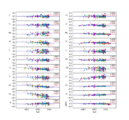
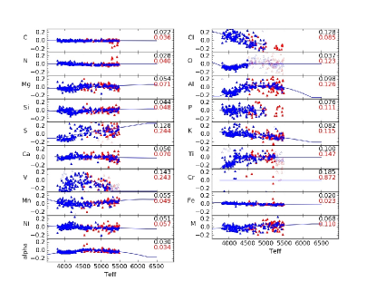
As was the case for DR12, we find that the derived abundances of some of the individual elements show a small dependence on effective temperature for stars within a given star cluster. Assuming that abundances are homogeneous within clusters (e.g., Bovy 2016, De Silva et al. 2006, 2007), such a dependence might result from effects that are not well characterized by our models, such as NLTE effects, or effects from blending that are a function of temperature. Under the assumption of homogeneity, we apply a small internal calibration to the derived abundances as a function of $T_{\rm eff}$, using a set of star clusters to derive this calibration. We have chosen to employ only clusters with metallicity greater than [M/H]$>$ -1, because this is representative of the vast majority of the APOGEE stars; this restricts the sample to mostly open clusters. Unlike DR12, in DR13 and DR14 we fit for a $T_{\rm eff}$  dependence of [X/M] rather than the [X/H] that was used for DR12 because the scatter in the [X/M] vs $T_{\rm eff}$ relations is smaller. As in DR12, no internal calibration is made for C or N because these cannot be assumed to be homogeneous within clusters along the giant branch because of mixing.

The observed cluster stars cover a more limited range of effective temperature than that of the full sample. In an effort to remove effective temperature dependences over a larger range of the APOGEE data, we inspected [X/M] vs $T_{\rm eff}$  diagrams for each element for a subsample of the APOGEE data with $70<l<110$, which limits the stars to be at Galactocentric radii not dramatically different from the solar radius, under the assumption that there should not be a temperature dependence of abundance ratios within this sample. We note that this sample was not used to derive the effective temperature dependence of the calibration relations, but only to inspect what different calibration relations from the cluster fits (different orders and $T_{\rm eff}$  limits for the fit) had an impact on the [X/M] locii; we adopted the calibration that most effectively removed any effective temperature trends.

Separate calibration relations were derived for giants and for dwarfs, where equation 6 was used to classify stars as giants or dwarfs. For most elements, no calibration was applied to stars cooler than 3500 K because of the lack of calibrators and because the extrapolation of the calibration did not appear to work well judging from the solar circle sample, although we do provide calibrated values for a few elements for which the extrapolation looked reasonable.

In addition to internally calibrating the abundances as a function of $T_{\rm eff}$, we also adopted a zeropoint shift to force the mean abundance ratios of all observed stars with -0.1$<$[M/H]$<$0.1, $-5<|b|<5$, and $70<l<110$ to be zero, i.e., we forced the mean abundance ratio of stars near the solar circle within $\pm 0.1$ of the solar abundance to have solar abundance ratios. This is motivated by studies of the solar neighborhood (e.g., Bensby et al. 2014) that suggest that most stars in the solar neighborhood have solar abundance ratios at solar abundance. Such an assumption could be questioned, but given the internal calibration with $T_{\rm eff}$, we have to adopt some [X/M] zeropoint (DR12 simply adopted the raw abundance at $T_{\rm eff}$$=$ 4500 K). The need for zeropoint corrections might result from issues with the astrophysical $\log gf$ values, e.g., from incorrect assumed abundances for Arcturus and/or the Sun.

6.3.1 DR13

Calibration relations for DR13 elemental abundances are presented in Appendix A.3. We note that abundances for Nd and Y show large scatter in clusters for both dwarf and giants, potentially indicating that windows used in determining the chemical abundances are not ideal. These elements are derived from weak, blended features in the spectra that are likely not present in stars with $T_{\rm eff}$ $\gtrsim$ 4200 K (see e.g., Hasselquist et al. 2016). Moreover, it was later discovered that Y abundances were actually derived from a spectral line that was actually due to a transition of Yb (see e.g., Hawkins et al. 2016). While we do provide raw values for Nd and Y, these values do not represent the abundance of these elements and should not be used.

Rb, Cu, and Ge show strong temperature trends, and while calibrated abundances are provided, they should probably not be used. A detailed analysis of the two Rb I lines used for the DR13/DR14 abundances reveals that both lines are almost certainly affected significantly by blends, with the bluer Rb I line blended with a CN line and the redder Rb I line blended with an unclassified, high-excitation Fe I line. Inspection of the single germanium line in the APOGEE spectral window (Ge I at $\lambda$=16759.76Å_Air) finds that this line is very weak.

6.3.2 DR14

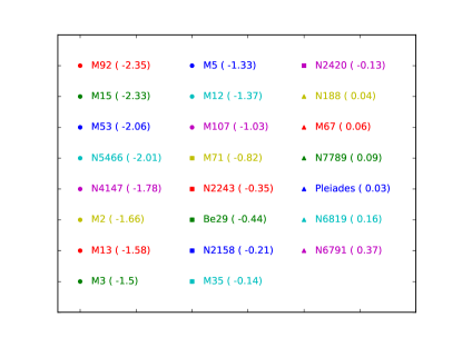
Figures 16 and 17 show the internal calibration relations for red giants and dwarfs for DR14, as derived from cluster stars. Figure 18 lists the clusters that were used and the symbols that represent them in Figures 16 and 17. In general, the trends with $T_{\rm eff}$  are small, with the largest slopes occuring in giants for Na, Ti, Cr, Mn, and Co.

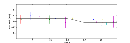
Figure 15 compares the mean derived [M/H] from cluster stars with cluster metallicities from the literature. While different studies do not always agree on cluster metallicities, the raw ASPCAP [M/H] for metal poor clusters is $\sim$ 0.15 dex higher than most literature values. As a result, we applied a simple calibration of a constant offset at [M/H]$<$-1, with a linear ramp to zero correction at [M/H]$>$-0.5. Note that while we applied this external correction to [M/H], we did not apply it to [Fe/H].

Table 5 show the zeropoint offsets applied to each of the individual element abundances based on the solar circle sample, for both giants and dwarfs and for DR13 and DR14. In general these zeropoint shifts are modest ($<0.1$ dex), with the exceptions of Na, Al, Si, and V. Future line list work will attempt to understand whether there are plausible reasons for these that can be addressed.

Figure 15: Mean [M/H] of cluster stars compared with cluster metallicities from the literature, and derived [M/H] calibration. Different point colors and symbols are used to distinguish different clusters.

While raw abundance measurements using the Rb, Cu, Ge, Y (Yb!), and Nd windows were made for DR14, no calibrated abundances of these elements are presented because of the challenges/problems involved with measuring the relevant lines (discussed above), and we do not recommend the use of these abundances with the current analysis.

Similarly, a more in depth analysis of the Na windows have revealed that the Na features are not measurable at [M/H] $<$ -1.0 so, as a result, we do not provide calibrated abundances of Na for metal-poor stars.

Table 5: Elemental abundance zeropoint offsets

Element	DR14		DR13
	giants	dwarfs	giants	dwarfs
C	0.000	0.000	0.000	-0.019
CI	0.000	-0.038	0.000	-0.026
N	0.000	-0.003	0.000	-0.010
O	0.035	0.020	0.060	0.068
Na	0.103	$\cdots$	0.186	0.096
Mg	0.022	-0.035	0.045	-0.003
Al	0.208	0.053	0.108	0.043
Si	0.127	-0.034	0.107	-0.023
P	0.003	0.000	-0.008	0.000
S	0.003	-0.074	-0.092	-0.017
K	-0.046	0.001	-0.026	-0.029
Ca	-0.027	0.045	-0.021	0.023
Ti	0.016	0.049	-0.014	-0.002
TiII	0.090	$\cdots$	0.166	0.000
V	0.142	0.186	0.110	0.002
Cr	-0.137	-0.066	-0.057	-0.044
Mn	0.012	-0.106	0.041	-0.077
Fe	0.003	0.023	-0.005	0.016
Co	-0.061	$\cdots$	0.003	0.000
Ni	-0.005	0.047	-0.001	0.030
Cu	$\cdots$	$\cdots$	0.452	0.026
Ge	$\cdots$	$\cdots$	0.354	0.000
$\alpha$	0.038	0.027	0.056	-0.004

Figure 16: DR14 internal abundance calibrations for giants applied as a function of $T_{\rm eff}$. Each panel shows the results for abundances in calibration clusters along with the adopted calibration relation (line). Different colors and point types are used to distinguish different clusters as denoted in Figure 18. Number in the upper right gives residual scatter around the calibration relation; red number is scatter for M67 stars only.

Figure 17: As Figure 16, but for dwarfs.

Figure 18: List of clusters used for internal calibration, with associated symbols used in Figures 16 and 17.

Estimated uncertainties in abundances were derived using the same methodology as for DR12. We use the abundance derivations in both open and globular cluster stars (removing known second generation stars from the latter) with the underlying assumption that individual element abundances are uniform in all cluster members (apart from C and N). In the selected cluster sample, we measure the element abundance scatter in [X/M] in bins of effective temperature, metallicity, and signal-to-noise (S/N). For each individual element, we fit these values with a simple functional form:

$$log\sigma σ=A+B(T_{eff}-4500)+C(S/N-100)+D[M/H]$$ (13)

where $\sigma$σ is the scatter among cluster stars relative to the mean derived abundance. The $S/N$ used in this relation is capped at $S/N=200$. Note that in the above relation, the fit to log ensures that the derived relation will always yield a positive uncertainty. The values for the coefficients (A, B, C, D) associated with each element for giants are given in Table 6.

The abundance precision for [Fe/H] is underestimated by this methodology since the scatter is computed from [Fe/M], but the measurement of [M/H] is strongly dominated by Fe lines, so [Fe/M] will show very little scatter.

As another estimate of uncertainty, we also include in Table 6 the “global” uncertainties, which represent the total scatter around the effective temperature fits shown in Figures 16 and 17. For Fe, we calculate this in [Fe/H] to avoid the problem mentioned above. However, these global uncertainties do not capture the dependence on $T_{\rm eff}$, [M/H], and S/N.

Table 6: Parameters for DR14 abundance uncertainties.

El	A	B	C	D	$\sigma$	$\sigma_{global}$
C	-3.488	9.42E-04	-1.93E-03	-0.685	0.030	—
C I	-3.010	4.24E-04	-2.82E-03	-0.567	0.049	—
N	-3.138	8.24E-04	-1.20E-03	-0.632	0.043	—
O	-3.454	8.48E-04	-3.15E-03	-0.649	0.031	0.039
Na	-2.413	4.62E-04	-2.84E-03	-0.188	0.089	0.132
Mg	-3.826	-7.13E-05	-2.50E-03	-0.693	0.021	0.039
Al	-2.974	6.91E-04	-2.00E-03	-0.345	0.051	0.081
Si	-3.643	3.17E-04	-1.60E-03	-0.473	0.026	0.037
P	-2.233	3.10E-04	-2.59E-03	-0.149	0.10	0.130
S	-2.704	1.12E-04	-3.68E-03	-0.453	0.066	0.062
K	-2.966	2.52E-04	-5.55E-03	-0.467	0.051	0.061
Ca	-3.510	2.02E-04	-5.21E-03	-0.634	0.029	0.038
Ti	-3.243	5.48E-04	-2.68E-03	-0.508	0.039	0.064
Ti II	-2.386	4.63E-04	-1.49E-03	-0.188	0.092	0.147
V	-2.626	6.87E-04	-2.50E-03	-0.381	0.072	0.117
Cr	-3.100	4.30E-04	-4.13E-03	-0.626	0.045	0.071
Mn	-3.424	3.30E-04	-4.60E-03	-0.582	0.032	0.054
Fe	-4.757	-1.80E-04	-8.32E-04	-0.443	0.009	0.047
Co	-2.469	7.21E-04	-4.16E-03	-0.065	0.084	0.141
Ni	-3.779	2.84E-04	-5.71E-03	-0.659	0.022	0.024
Rb	-2.434	-4.91E-05	-8.50E-04	0.071	0.087	—
M	-3.667	5.80E-04	3.98E-04	-0.568	0.025	0.035
$\alpha$	-4.284	2.10E-05	-1.45E-03	-0.793	0.013	0.014

6.4 Derived parameters and abundances

6.4.1 Comparison of DR12, DR13, and DR14

To illuminate the differences that result from modifications in the analysis, Figure 19 compares the calibrated stellar parameters between DR12, DR13, and DR14, for high S/N ($S/N>150$) stars that overlap between the releases. Figure 20 compares the calibrated elemental abundances.

Figure 19: Comparison of calibrated stellar parameters from DR12, DR13, and DR14 for stars that overlap. Points are color-coded by [M/H].

Figure 20: Comparison of calibrated elemental abundances from DR12, DR13, and DR14 for stars that overlap. Points are color-coded by [M/H].

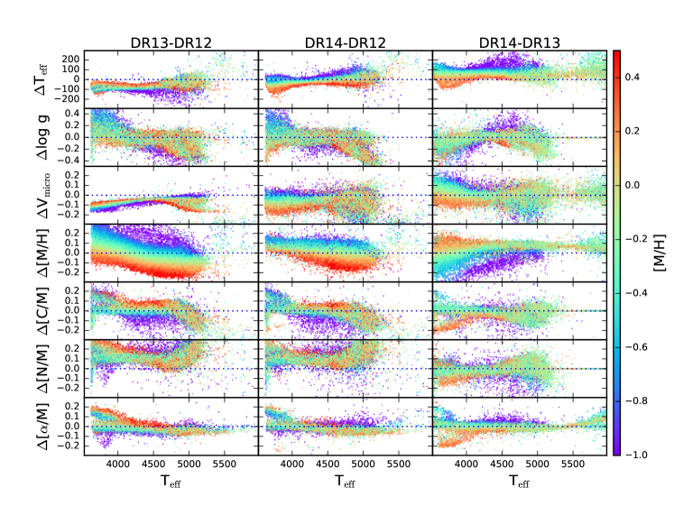
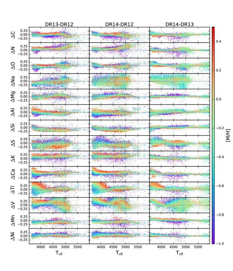
As described in previous sections, differences include changes in the line list (from DR12 to DR13/DR14), changes in the handling of microturbulence, changes in continuum normalization, and changes in calibration. It is apparent that changes in the analysis and calibration make a difference in the derived results; we hope and believe that the changes are in the direction to make things more accurate. In general, there is a larger difference between DR12 and DR13 than there is between DR13 and DR14, which is not surprising given the larger changes in the analysis between DR12 and DR13, e.g., different line list and synthesis. Differences in $T_{\rm eff}$, $\log{g}$, microturbulent velocity, and [M/H] arise from different calibration choices as much as from analysis differences.

6.4.2 Comparison with independent measurements

To provide independent assessment of the accuracy of the DR13 and DR14 parameters and abundances, we compiled a set of independent measurements of stellar parameters and abundances derived from optical spectra and analysis for a subset of APOGEE stars. These are presented and discussed in Jönsson et al. (2018), a companion paper to this work. Here we present a brief summary, and we direct the reader to Jönsson et al. (2018) for a complete description.

Jönsson et al. (2018) find the same trend of APOGEE/ ASPCAP $T_{\rm eff}$ with metallicity as discussed in comparison to the photometric $T_{\rm eff}$ above. As expected, this effect is much smaller for DR14 when a calibration was applied to take care of this problem. However, the optical spectroscopic effective temperatures suggest that even the calibrated DR14 $T_{\rm eff}$  is still about 100 K too high for high-metallicity stars. The other (calibrated) stellar parameters show no trends or systematic offsets for giants.

For most of the abundances – C, Na, Mg, Al, Si, S, Ca, Cr, Mn, Ni – the DR14 ASPCAP analysis have systematic differences to the comparisons samples of less than 0.05 dex (median), and random differences of less than 0.15 dex (standard deviation). Magnesium is the most accurate alpha-element, showing a very clear thin/thick disk separation, and nickel is the most accurate iron-peak element.

Some abundances – N, O, K, Ti I, V, Co – have differences with the optical abundances that are correlated with stellar parameters. Given the systematic trends of $T_{\rm eff}$ with metallicity, some of these abundances might be improved if the calibrated $T_{\rm eff}$  were used instead of the uncalibrated $T_{\rm eff}$, especially for elements where the derived abundances are a strong function of the adopted $T_{\rm eff}$  such as Ti I.

Some elemental abundances – P, Cu, Ge, Rb, Nd, Yb – are not evaluated in Jönsson et al. (2018) due to either lack of comparison samples with overlapping stars/element or due to the APOGEE-analysis of the elements being unreliable in the present analysis.

Future data releases will consider these issues, which will hopefully lead to better stellar parameters as well as abundances.

7 Persistence

As discussed in §3.1 and 3.5.2, several modifications were made to the pipeline to reduce the impact of persistence on the data. Persistence is mostly relevant for the data taken before Fall 2014, when the “blue” chip was replaced (although there is evidence for some persistence in parts of the “green” chip as well).

To assess whether these modifications had an impact on the resulting stellar parameters and abundances, we repeat the same comparison of parameters and abundances for stars unaffected by persistence with stars most affected by persistence that was performed in Holtzman et al. (2015). Persistence is most likely to affect faint stars, so we are probing maximal effects by investigating a subsample with $H>12$. Figures 21, 22, 23, 24 show locii of parameters and abundances for three samples: stars with no persistence flags set (left panel), stars with PERSIST_HIGH flag set for some, but not all visits (middle panel), and stars with PERSIST_HIGH flag set in all visits. As described above, one of the significant changes was to reduce the weight of pixels affected by persistence in the visit combination. Given this procedure, we expect significant improvement for stars in which only some of the visits had persistence, as these will contribute little to the combined spectra; even for stars with persistence in all visits, we expect improvements because the reduced weights mean that persistence-affected pixels will carry less weight in the ASPCAP fits than other pixels.

Figure 21: HR diagrams for 3 subsamples split by persistence behavior: left panel has stars that are not flagged as having significant number of persistence-affected pixels in any of the visits, middle panel has stars that are flagged with significant persistence-affect pixels in some visits, and right panel has stars that are flagged with significant persistence-affected pixels in all visits. Points are color-coded by [M/H].

Figure 22: CNO abundances relative to Fe for the same subsamples presented in Figure 21. Points are color-coded by $T_{\rm eff}$.

Figure 23: Same as Figure 21, but for $\alpha$-element abundances relative to Fe.

Figure 24: Same as Figure 21, but for other element abundances relative to Fe.

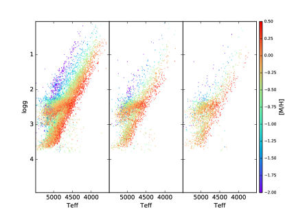
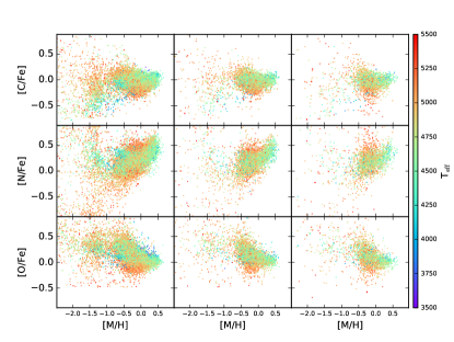
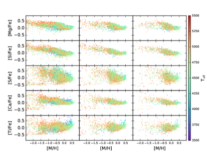
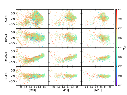
The results presented in Figure 21–24 suggest that there is little difference in the derived parameters and abundances between the different subsets, suggesting that we have significantly reduced the effect of persistence on derived parameters and abundances. Interested readers can compare these plots with Figures 15-18 in Holtzman et al. (2015).

Jahandar et al. (2017) have recently presented data for a few stars that clearly demonstrate very poor results in APOGEE DR12 that result from persistence; they claim that some of the poor results persist in DR13. In general, however, we find no evidence that persistence strongly affects results of a significant fraction of the APOGEE sample in DR14. The low metallicity ([Fe/H] = -0.6), warm temperatures ($T_{\rm eff}$= 4800 K), and faintness (H $>$ 14) of the targets in Jahandar et al. (2017) lead to multiple issues, including problems in the RV determination and ASPCAP pipeline. For a boutique analysis, correction of the persistence and careful RV combination (as was done by Jahandar et al. (2017)) will make a significant difference.

While we believe that significant improvements in persistence handling have been made in DR14, users are reminded that the presence of a significant number of persistence-affected pixels in the spectrum of an object is flagged in the stellar catalog files/tables with the STARFLAG bitmask (significant fraction pixels affected in any of the component visit spectra) and the ANDFLAG bitmask (significant fraction in all of the component visit spectra). In the spectra themselves, pixels known to be affected by persistence are flagged in the PIXMASK.

8 Results from The Cannon

DR14 includes, for the first time, an alternate set of stellar parameters and abundances as derived from a data driven method called The Cannon (Ness et al., 2015; Casey et al., 2016). This technique parameterizes the spectral fluxes as a function of a set of externally-determined stellar parameters and abundances; in principle these could be any physical quantities, so are generically referred to as labels. The method uses a training set of stellar spectra to determine the coefficients of the parameterization that best match the training set spectra, and these are then applied to a broader data set to derive labels for a larger data set. The method has the power of exploiting all of the information that may be present in the stellar spectra. In general, it has been claimed that the method produces higher precision than the ASPCAP results (e.g., Ness et al. 2017). This is plausible because the method can respond to individual features in the spectra that we may not model well with the ASPCAP analysis, e.g., lines with imperfect atomic data, lines missing from the line list, lines that are not well modeled with the 1D LTE approach used by ASPCAP, etc. For more details, refer to the papers listed above.

For DR14, Cannon results have been determined using the Cannon-2 code (Casey et al., 2016), except that we used a different prescription for the uncertainties in the input spectra. Specifically, we adopted the same uncertainties used in the ASPCAP pipeline. In particular, these uncertainties use better knowledge of the sky spectra to mask broader regions around sky lines that are often imperfectly subtracted.

We initially ran The Cannon after training a model on the ASPCAP stellar parameters and abundances and found that it appeared to give higher precision, based on the tightness of locii in, e.g., plots of [X/M] as a function of [M/H]. However, we subsequently used the model to generate spectra, varying individual elemental abundances one at a time, and found that the resulting spectra showed variations where no identified lines of the element in question were found and, in fact, in some cases, where identified lines of other elements were found. As a result, it appeared that The Cannon was training on features of multiple elements that may be well correlated in the bulk of the training set. This is in some sense not surprising, and in some situations might actually be desired: if we were interested in a single label that has a complicated — and not fully described — relationship with other labels (e.g., age), then we might want The Cannon to be building on all information available. If the training set is representative of the test sets, then correlated information can be useful.

This behavior, however, may jeopardize the ability of the model to derive abundances for stars that might have slightly different abundance patterns; in fact, the ability to distinguish these is a key goal of the APOGEE project. To prevent this, for the labels that are associated with individual elemental abundances, we use “censoring” in The Cannon parameterization, which means that we only allow pixels that we expect, based on our line list, to be affected by the abundance of the element. This minimizes the potential issue of having correlations of abundances of different elements in the training set imposing such correlations on the full data set. In practice, we implemented this by only allowing The Cannon to use pixels that have non-zero weight in the windows used by FERRE for the ASPCAP abundances, although we note that these windows may not perfectly include all wavelengths affected by the abundance of any given element.

Using this wavelength sensoring changes The Cannon results significantly. An extreme example of the difference between censored and uncensored results can be seen by comparing Figure 25, which shows Cannon (bottom) and ASPCAP (top) results for [Ca/Fe], with Figure 26, which shows the same thing for the censored results. For calcium, while the uncensored Cannon results look tighter than the ASPCAP results, the censored results look significantly worse. This is not true in general: for some elements, even the censored Cannon results look tighter than the ASPCAP results. For example, Figure 27 and 28 show the same comparison for [Ni/Fe], for which even the censored Cannon results look better. The reasons for both of these extremes (e.g., significantly worse [Ca/Fe] than ASPCAP and significantly better [Ni/Fe] than ASPCAP) are still being fully investigated, and these efforts are expected to improve both approaches.

Figure 25: Uncensored Cannon results for Ca compared with ASPCAP results for stars with 4000 $<$ $T_{\rm eff}$$<$ 4500 at a range of S/N. Points are color-coded by the $\chi^{2}$ of the fit.

Figure 26: Same as Figure 25 but for censored Cannon results.

Figure 27: Uncensored Cannon results for Ni compared with ASPCAP results, for stars with 4000 $<$ $T_{\rm eff}$$<$ 4500 at a range of S/N. Points are color-coded by the $\chi^{2}$ of the fit.

Figure 28: Same as Figure 27 but for censored Cannon results

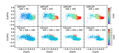
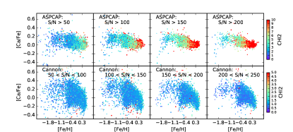
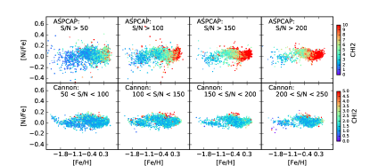
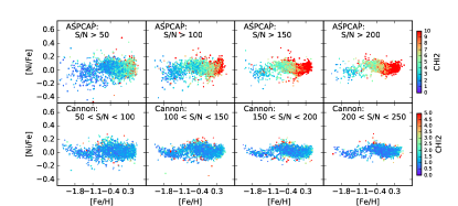
In practice, we apply the following steps to derive Cannon labels:

1. The combined apStar spectra are normalized, following the prescription in Casey et al. (2016).

2. A training set is constructed that attempts to sample a wide range of stellar parameters: we split the $T_{\rm eff}$-$\log{g}$-[M/H]  space into cubes covering the range 3500$<$$T_{\rm eff}$$<$5500, 0$<$$\log{g}$$<$3.9, and -2.5$<$[M/H]$<$0.5, and take the 50 stars with the highest S/N in each cube: this results in a training set of 1464 stars. For the labels of this subsample, we adopt the calibrated ASPCAP $T_{\rm eff}$, $\log{g}$, [M/H], [$\alpha$/M], and [X/H] for 20 different elements. Note that we restrict the training set to giants, both because of increasing uncertainties in (or lack of) the ASPCAP calibration relations, and also because with a broader range of stellar parameter, the quadratic parameterization used by the Cannon-2 is likely to be less accurate.

3. We train The Cannon on this sample, using wavelength censoring for the labels that refer to individual element abundances. We adopt the ASPCAP windows for the individual elemental abundances as the wavelength censors.

4. We apply the derived model to the remainder of the ASPCAP data set for objects whose ASPCAP parameters fall within the range of the parameters adopted for the training set.

8.0.1 Using Cannon labels

All of the issues/caveats associated with ASPCAP apply to The Cannon results, as The Cannon abundances depend on the abundances of the training set which are derived using ASPCAP. The Cannon provides a $\chi^{2}$ value which indicates how well The Cannon model spectrum fits the observed spectrum. Results with higher $\chi^{2}$ are significantly more uncertain.

9 Datamodel revisions

As in previous data releases, APOGEE data are released through files in the science archive server (SAS), including summary data files (allVisit and allStar) that include the main APOGEE derived quantities (radial velocities, stellar parameters, and elemental abundances), and all of the pipeline data products, include the final combined spectra (apStar) and pseudo-continuum normalized spectra (aspcapStar). The derived quantities are also available in the Catalog Archive Server (CAS), an online database.

Several modifications have been made to the derived quantities that are presented in the SAS summary files and the CAS tables.

• Since APOGEE-2 data use a different set of targeting flag bits than APOGEE data (see Zasowski et al. 2017 for details), DR14 includes the APOGEE target flags (APOGEE_TARGET1 and APOGEE_TARGET2) and the APOGEE-2 target flags (APOGEE2_TARGET1, APOGEE2_TARGET2, and APOGEE2_TARGET3); the APOGEE values are zero (no bits set) for APOGEE-2 targets, and vice versa

• Since some stars may have ASPCAP fits from multiple synthetic grids (those near the grid boundaries), the allStar file and CAS table include an ASPCAP_CLASS entry that gives the grid that provided the best fit. The class names include the temperature code (F, GK, or M), a code for giant (g) or dwarf (d) grid, and a code for the LSF used (abcd). In the allStar file, there are arrays, FPARAM_CLASS and CHI2_CLASS, that give the raw parameters and $\chi^{2}$ values for each fit that was performed on a given star.

• In the DR12 allStar file, abundances were provided in arrays labeled FELEM (uncalibrated) and ELEM (calibrated), as well as in labels with individual elemental abundance names. However, the array values were a bit complicated to interpret, since some of the abundances were given as [X/H], while others were given as [X/M], depending on the grid dimension used for the abundance fit. In DR13 and DR14, the FELEM array has been preserved, but the ELEM array has been removed: calibrated abundances are presented in both X_M and X_H arrays (with abundances relative to M and H, respectively), as well as in labels with individual element abundance names, relative to iron (e.g., C_FE, MG_FE, NI_FE).

As before, raw parameters are loaded into the FPARAM array, with calibrated parameters loaded in a PARAM array and also into named tags TEFF, LOGG, VICRO, M_H, ALPHA_M, C_M, N_M, and VSINI (C_M and N_M for giants only, VSINI for dwarfs only). If stars are outside the range for which calibration objects are available, the calibrated and named quantities are set to a value of -9999. One important implication of this is that dwarfs do not have the LOGG tag populated; the raw ASPCAP LOGG is available in the second element of the FPARAM array.

9.0.1 Cannon data products

In the SAS, DR14 includes a summary allStarCannon file, as well as cannonField and cannonStar files, as described in the following paragraphs.

The allStarCannon file bundles up all of The Cannon results in a single file, analogous to the allStar file with ASPCAP results. The allStarCannon file has been constructed to be a line-for-line match with the allStar file, to make it simple to use either ASPCAP or Cannon results, or to compare them. However, the allStarCannon file does not repeat all of the information contained in the allStar file; it simply supplements it with Cannon label results. Note that the allStarCannon files do not have Cannon abundances for many stars, since Cannon results are only provided for stars that fall within The Cannon training parameter space; we carry along empty Cannon values for the other stars to preserve the simple line-to-line matching between the allStar and allStarCannon files.

The cannonField files bundle up all of the results for stars in a given field and are analogous to the aspcapField files. These files contain the spectra and derived best fits, as well as the derived label values, in a FITS table format file (see the cannonField data model).

The cannonStar files contain the results for individual stars, including labels, normalized spectra, uncertainties, and best fit spectra, in a FITS image format (see the cannonStar data model).

For convenience of users who might want to delve deeper into and experiment with The Cannon results, the subset of stars used to train The Cannon are saved in a file (apogee-dr14-giants-xh-censor-training-set.fits) and the model itself is also saved (as a Python pickle file, apogee-dr14-giants-xh-censor.model).

In the CAS, The Cannon results can be found in the cannonStar table.

10 Conclusions

We have described the methodology used for the SDSS/APOGEE Data Releases 13 and 14, concentrating on the areas in which they differ from that of DR12 (Holtzman et al., 2015). Improvements have been made in the data reduction in the areas of telluric correction, persistence, and radial velocity determination. Methods for determining the stellar parameter and abundance determinations were refined.

We describe the calibrations applied to the stellar parameters and abundances in SDSS/APOGEE DR13 and DR14. We also describe some of the shortcomings of these calibrations and suggest alternate calibrations for $T_{\rm eff}$ in DR13, and for $\log{g}$  in both DR13 and DR14.

Analysis of stars within open clusters suggests that the precision of the abundances is typically 0.05 dex. A companion paper (Jönsson et al., 2018) presents a comparison of the calibrated parameters and abundances with independent optical measurements for an overlapping sample, and finds that the systematic differences for most elements in DR14, when compared to the references, are of the order of 0.05 dex.

We demonstrate that the modifications made in the pipeline to reduce the effect of persistence seem to be generally effective.

We have also described and presented results using analysis by the Cannon (Ness et al., 2015). We find that if we allow The Cannon to train without any restriction on what part of the spectrum it uses for elemental abundances, it can use regions where there are not any known features of the element in question and in many cases, seems to be using features of other elements. As a result, we run The Cannon in “censored” mode where we only allow it to use regions of the spectrum for each element where lines of that element are known. In this mode, The Cannon results can have considerably larger scatter than results from uncensored mode, and in some cases, larger scatter than the ASPCAP results.

Future data releases will likely include further improvements. In particular, we are working towards stellar parameter and abundance determination with a homogeneous grid of model atmospheres across the full temperature range. We are improving the line list to include hydrides that are important for cool dwarfs and to include lines of several s-process elements (Hasselquist et al. 2016, Cunha et al. 2017). We are also working to provide better abundance determinations for elements whose lines are blended with other elements in the same element group.

Funding for the Sloan Digital Sky Survey IV has been provided by the Alfred P. Sloan Foundation, the U.S. Department of Energy Office of Science, and the Participating Institutions. SDSS acknowledges support and resources from the Center for High-Performance Computing at the University of Utah. The SDSS web site is www.sdss.org.

SDSS is managed by the Astrophysical Research Consortium for the Participating Institutions of the SDSS Collaboration including the Brazilian Participation Group, the Carnegie Institution for Science, Carnegie Mellon University, the Chilean Participation Group, the French Participation Group, Harvard-Smithsonian Center for Astrophysics, Instituto de Astrofísica de Canarias, The Johns Hopkins University, Kavli Institute for the Physics and Mathematics of the Universe (IPMU) / University of Tokyo, Lawrence Berkeley National Laboratory, Leibniz Institut für Astrophysik Potsdam (AIP), Max-Planck-Institut für Astronomie (MPIA Heidelberg), Max-Planck-Institut für Astrophysik (MPA Garching), Max-Planck-Institut für Extraterrestrische Physik (MPE), National Astronomical Observatories of China, New Mexico State University, New York University, University of Notre Dame, Observatório Nacional / MCTI, The Ohio State University, Pennsylvania State University, Shanghai Astronomical Observatory, United Kingdom Participation Group, Universidad Nacional Autónoma de México, University of Arizona, University of Colorado Boulder, University of Oxford, University of Portsmouth, University of Utah, University of Virginia, University of Washington, University of Wisconsin, Vanderbilt University, and Yale University.

JAH, SRM, and VVS acknowledge support for this research from the National Science Foundation (AST-1109178). SRM also acknowledges NSF grant AST-1616636). JAJ and MP acknowledge support from NSF grant AST-1211673. SzM has been supported by the Premium Postdoctoral Research Program of the Hungarian Academy of Sciences, and by the Hungarian NKFI Grants K-119517 of the Hungarian National Research, Development and Innovation Office. HJ acknowledges support from the Birgit and Hellmuth Hertz’ Foundation (via the Royal Physiographic Society of Lund), the Crafoord Foundation, and Stiftelsen Olle Engkvist Byggmästare.

Appendix A DR13 calibrations

Here we present proposed revisions to the calibrations used for DR13.

A.1 Effective temperature

No calibration was applied to the spectroscopic $T_{\rm eff}$ in DR13. However, Figure 29 shows the difference between the spectroscopic temperature and photometric temperatures derived from the González Hernández & Bonifacio (2009) photometric calibration, as applied to a low-reddening sample that includes all APOGEE stars with $b>30$ and $E(B-V)<0.02$, where $E(B-V)$ is the Schlegel et al. (1998) reddening in the direction of the star. It is apparent that there is a large trend with metallicity, [M/H], with a substantial offset for metal-poor stars. This trend also exists in comparisons with other spectroscopic samples (e.g., Jönsson et al. 2018).

Figure 29: Difference between APOGEE DR13 $T_{\rm eff}$ and photometric $T_{\rm eff}$, demonstrating the problem with the DR13 $T_{\rm eff}$, for which no calibration was applied. Points show mean differences in bins of metallicity, and the line gives the derived fit that is recommended to apply to DR13 values. Points are color-coded by $T_{\rm eff}$.

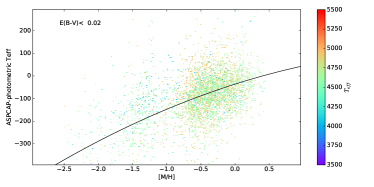
A fit to the low reddening sample yields the relation:

$$T_{eff}(ASPCAP)-T_{eff}(GHB)=-36.17+95.97[M/H]-15.09[M/H]^{2}$$ (A1)

where [M/H]  is the calibrated ASPCAP metallicity, as shown in Figure 29. We suggest that if DR13 users are interested in effective temperatures, equation A1 should be adopted as a post-calibration to the DR13 release values.

For DR13, all stars were assigned a fixed $T_{\rm eff}$ uncertainty, which was determined from the scatter in the relation between $T_{\rm eff}$ and photometric $T_{\rm eff}$, reduced by a factor of $\sqrt{2}$ to account for uncertainties in the photometric effective temperatures: this corresponds to $\sim$ 70 K. This scatter is dominated by stars near solar metallicity, so is not strongly affected by the possible systematics at low metallicity discussed above.

A.2 Surface gravity

Figure 30 shows the difference between the ASPCAP DR13 surface gravities and asteroseismic gravities for stars from the APOKASC 3.6.0 catalog (Pinsonneault et al., 2014), which includes significantly more stars with asteroseismic values than were available for DR12. This comparison suggests that there is a significant trend with metallicity (top panel), not much trend in surface gravity (middle panel), and a notable difference between the RGB and RC (lower panel).

Figure 30: Left plot shows comparison of the DR13 surface gravity with asteroseismic surface gravity. Top panel shows difference as a function of metallicity with points color-coded by surface gravity, middle panel shows difference as a function of surface gravity color-coded by metallicity, and bottom panels shows difference for RGB and RC. Right panel shows calibration of DR13 ASPCAP surface gravities with asteroseismic and physical (clusters) gravities; points are color-coded by temperature. Large points show the median difference with physical gravities in clusters (red before effective temperature correction, green after correction, blue adopting photometric effective temperature. Top panel shows comparison with raw ASPCAP surface gravities; bottom panel after DR13 surface gravity calibration.

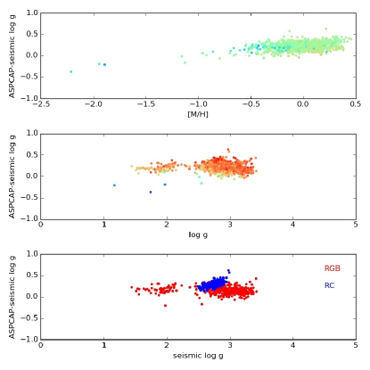
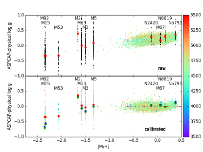
For DR13, we adopted a $\log{g}$ correction that depends both on surface gravity and metallicity. We note that this differs significantly from DR12, where only a surface gravity dependence was found and calibrated.

We also derived a separate correction for the ASPCAP $\log{g}$ values from RGB and RC stars. Based on the asteroseismic sample, we have derived a relation that allows us to classify the stars correctly at 95% level, using $T_{\rm eff}$, [M/H], and [C/N] (Bovy et al. 2014, Pinsonneault, private communication). For every star, we compute the difference between the ASPCAP raw effective temperature and a fiducial metallicity-dependent ridgeline derived by Bovy et al. (2014):

$$T_{ridge}=4468+(\log g-2.5)/0.0018–382.5[M/H]$$ (A2)

Stars cooler than the ridgeline temperature are classified as RGB stars, while stars more than 100 K hotter than the ridgeline temperature are classified as RC stars. For stars in the intermediate region, the observed C/N ratio is used to help to discriminate RGB from RC stars. Stars with

$$[C/N]<-0.113-0.0043(T-T_{ridge})$$ (A3)

are classified as RGB stars, while stars with

$$[C/N]>-0.088-0.0018(T-T_{ridge})$$ (A4)

are classified as RC stars. For stars in an ambiguous region in C/N space, we interpolate between the RGB and RC corrections.

The adopted surface gravity calibrations are then applied as follows. For RGB stars:

$$\log g=\log g(raw)-(0.300-0.048\log g+0.147[M/H])$$ (A5)

For RC stars:

$$\log g=\log g(raw)-(-4.442+3.326\log g+0.147[M/H]-0.581(\log g)^{2})$$ (A6)

Due to limited availability of asteroseismic data when the calibration was frozen, we chose to clip the metallicity correction to [M/H]$>$-1.5, below which the sign of the correction appears to reverse (top panel of left figure in Figure 30. The inclusion of additional data suggests that this reversal is, in fact, correct. The same conclusion is drawn from analysis of clusters for which “physical” gravities can be obtained using:

$$g=4\pi GM\sigma T_{eff}^{4}/L$$ (A7)

where $M$ is the adopted mass of evolved stars in the clusters (from isochrones, based on cluster metallicity and age), and $L$ is their luminosity, which was derived from the $H$ magnitude, a bolometric correction taken from the PARSEC isochrones, and an adopted reddening and distance. The right panel of Figure 30 adds the cluster results to the surface gravity comparison, and demonstrates that the surface gravity correction really does change sign at low metallicity.

As a result of this additional analysis, we believe that the DR13 calibrated gravities are too low at [M/H]$<$ -1.5. A revision to the DR13 surface gravities is recommended for stars with [M/H]$<$ -1.5:

$$logg(\textrm{post calibration})=logg(calibrated)–0.5([M/H]+1.5)$$ (A8)

In DR13, quoted uncertainties for $\log{g}$ are the observed scatter in the relation between raw $\log{g}$ and asteroseismic $\log{g}$, which corresponds to 0.08 for most stars; for stars in the intermediate region where the classification between RGB and RC was more uncertain, we adopted 0.095.

A.3 DR13 elemental abundances

Figure 31 presents the calibration relations that were adopted for the internal calibration relations for red giants and dwarfs in DR13.

Figure 31: DR13 internal abundance calibrations for red giants (left) and dwarfs (right) applied as a function of $T_{\rm eff}$. Different point colors and symbols indicate different clusters.

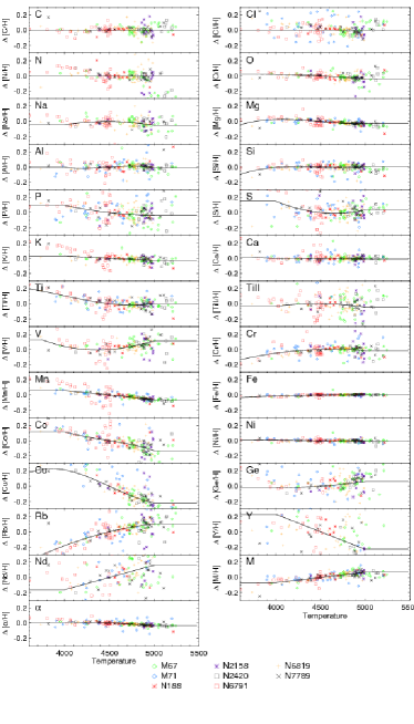
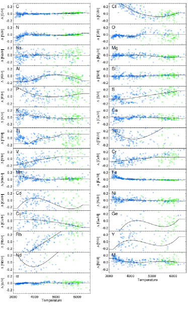
Estimated uncertainties in abundances were derived using the same methodology as for DR12. We use the abundance derivations in both open and globular cluster stars (removing known second generation stars from the latter) with the underlying assumption that individual element abundances are uniform in all cluster members (apart from C and N, which have mixing effects in giants). We have chosen to employ only clusters with metallicity greater than [M/H]$>$ -1, which restricts the sample to mostly open clusters. In the selected cluster sample, we measure the element abundance scatter in bins of temperature, metallicity, and signal-to-noise (S/N). For each individual element, we fit these values with a simple functional form:

$$log\sigma σ=A+B(T_{eff}-4500)/1000.+C[M/H]+D(S/N-100)/100.$$ (A9)

where $\sigma$σ is the scatter among cluster stars relative to the mean derived abundance. Note that in the above relation, the fit to log ensures that the derived relation will always yield a positive uncertainty. The values for the coefficients (A, B, C, D) associated with each element for giants are given in Table 7. Also included are the “Global” uncertainties, which represent the scatter around the temperature fits shown in Figure 31.

Table 7: Parameters for DR13 abundance uncertainties.

Element	A	B	C	D	$\sigma$	$\sigma_{global}$
C	-3.243	0.608	-0.757	-0.257	0.039	—
C I	-2.804	0.403	-0.743	-0.319	0.061	—
N	-2.671	0.373	-0.407	-0.192	0.069	—
O	-3.410	1.471	-0.778	-0.182	0.033	0.045
Na	-2.389	0.140	-0.926	-0.323	0.092	0.059
Mg	-3.980	0.284	-0.949	-0.115	0.019	0.029
Al	-2.616	-0.192	-0.628	-0.399	0.073	0.072
Si	-3.464	0.548	-0.482	-0.212	0.031	0.040
P	-1.988	0.384	-0.568	-0.369	0.137	0.120
S	-2.199	-0.030	-0.402	-0.295	0.111	0.122
K	-3.098	0.208	-0.583	-0.496	0.045	0.048
Ca	-3.520	0.153	-0.895	-0.405	0.030	0.032
Ti	-3.108	0.295	-0.741	-0.185	0.045	0.057
Ti II	-2.192	0.328	-0.538	-0.267	0.112	0.116
V	-2.447	1.030	-1.096	-0.519	0.087	0.089
Cr	-3.191	0.290	-0.775	-0.455	0.041	0.048
Mn	-3.523	0.235	-0.614	-0.488	0.029	0.049
Fe	-5.316	0.202	-0.874	0.019	0.005	0.053
Co	-2.062	1.064	-0.656	-0.523	0.127	0.095
Ni	-4.067	0.442	-0.816	-0.395	0.017	0.015
Cu	-2.140	-0.096	-0.559	-0.426	0.118	0.083
Ge	-1.893	0.258	-0.665	-0.395	0.151	0.107
Rb	-2.325	0.466	-1.117	-0.360	0.098	0.082
M	-3.730	0.232	-0.524	0.013	0.024	0.052
$\alpha$	-4.219	0.053	-0.794	-0.127	0.015	0.017

References

- Abolfathi et al. (2017) Abolfathi, B., Aguado, D. S., Aguilar, G., et al. 2017, ArXiv e-prints
- Allende Prieto et al. (2006) Allende Prieto, C., Beers, T. C., Wilhelm, R., et al. 2006, ApJ, 636, 804
- Alvarez & Plez (1998) Alvarez, R., & Plez, B. 1998, A&A, 330, 1109
- Asplund et al. (2005) Asplund, M., Grevesse, N., & Sauval, A. J. 2005, in Astronomical Society of the Pacific Conference Series, Vol. 336, Cosmic Abundances as Records of Stellar Evolution and Nucleosynthesis, ed. T. G. Barnes, III & F. N. Bash, 25
- Barber et al. (2006) Barber, R. J., Tennyson, J., Harris, G. J., & Tolchenov, R. N. 2006, VizieR Online Data Catalog, 6119
- Bensby et al. (2014) Bensby, T., Feltzing, S., & Oey, M. S. 2014, A&A, 562, A71
- Blanton et al. (2017) Blanton, M. R., Bershady, M. A., Abolfathi, B., et al. 2017, AJ, 154, 28
- Bovy (2016) Bovy, J. 2016, ApJ, 817, 49
- Bovy et al. (2011) Bovy, J., Hogg, D. W., & Roweis, S. T. 2011, Annals of Applied Statistics, 5
- Bovy et al. (2014) Bovy, J., Nidever, D. L., Rix, H.-W., et al. 2014, ApJ, 790, 127
- Casey et al. (2016) Casey, A. R., Hogg, D. W., Ness, M., et al. 2016, ArXiv e-prints
- Cunha et al. (2017) Cunha, K., Smith, V. V., Hasselquist, S., et al. 2017, ApJ, 844, 145
- De Silva et al. (2007) De Silva, G. M., Freeman, K. C., Asplund, M., et al. 2007, AJ, 133, 1161
- De Silva et al. (2006) De Silva, G. M., Sneden, C., Paulson, D. B., et al. 2006, AJ, 131, 455
- García Pérez et al. (2016) García Pérez, A. E., Allende Prieto, C., Holtzman, J. A., et al. 2016, AJ, 151, 144
- González Hernández & Bonifacio (2009) González Hernández, J. I., & Bonifacio, P. 2009, A&A, 497, 497
- Gunn et al. (2006) Gunn, J. E., Siegmund, W. A., Mannery, E. J., et al. 2006, AJ, 131, 2332
- Gustafsson et al. (2008) Gustafsson, B., Edvardsson, B., Eriksson, K., et al. 2008, A&A, 486, 951
- Hasselquist et al. (2016) Hasselquist, S., Shetrone, M., Cunha, K., et al. 2016, ApJ, 833, 81
- Hawkins et al. (2016) Hawkins, K., Masseron, T., Jofré, P., et al. 2016, A&A, 594, A43
- Holtzman et al. (2015) Holtzman, J. A., Shetrone, M., Johnson, J. A., et al. 2015, AJ, 150, 148
- Jahandar et al. (2017) Jahandar, F., Venn, K. A., Shetrone, M. D., et al. 2017, ArXiv e-prints
- Jönsson et al. (2018) Jönsson, H., others, et al. 2018, in preparation
- Koesterke (2009) Koesterke, L. 2009, in American Institute of Physics Conference Series, Vol. 1171, American Institute of Physics Conference Series, ed. I. Hubeny, J. M. Stone, K. MacGregor, & K. Werner, 73–84
- Majewski et al. (2017) Majewski, S. R., Schiavon, R. P., Frinchaboy, P. M., et al. 2017, AJ, 154, 94
- Massarotti et al. (2008) Massarotti, A., Latham, D. W., Stefanik, R. P., & Fogel, J. 2008, AJ, 135, 209
- Masseron & Hawkins (2017) Masseron, T., & Hawkins, K. 2017, A&A, 597, L3
- Ness et al. (2015) Ness, M., Hogg, D. W., Rix, H.-W., Ho, A. Y. Q., & Zasowski, G. 2015, ApJ, 808, 16
- Ness et al. (2017) Ness, M., Rix, H., Hogg, D. W., et al. 2017, ArXiv e-prints
- Nidever et al. (2015) Nidever, D. L., Holtzman, J. A., Allende Prieto, C., et al. 2015, AJ, 150, 173
- Pinsonneault et al. (2014) Pinsonneault, M. H., Elsworth, Y., Epstein, C., et al. 2014, ApJS, 215, 19
- Plez (2012) Plez, B. 2012, Turbospectrum: Code for spectral synthesis, Astrophysics Source Code Library
- Ramírez & Allende Prieto (2011) Ramírez, I., & Allende Prieto, C. 2011, ApJ, 743, 135
- Schlegel et al. (1998) Schlegel, D. J., Finkbeiner, D. P., & Davis, M. 1998, ApJ, 500, 525
- SDSS Collaboration et al. (2016) SDSS Collaboration, Albareti, F. D., Allende Prieto, C., et al. 2016, ArXiv e-prints
- Shetrone et al. (2015) Shetrone, M., Bizyaev, D., Lawler, J. E., et al. 2015, ApJS, 221, 24
- Wilson et al. (2018) Wilson, J., others, et al. 2018, in preparation
- Zamora et al. (2015) Zamora, O., García-Hernández, D. A., Allende Prieto, C., et al. 2015, AJ, 149, 181
- Zasowski et al. (2017) Zasowski, G., Cohen, R. E., Chojnowski, S. D., et al. 2017, AJ, 154, 198