Remote estimation over a packet-drop channel with Markovian state

Abstract

We investigate a remote estimation problem in which a transmitter observes a Markov source and chooses the power level to transmit it over a time-varying packet-drop channel. The channel is modeled as a channel with Markovian state where the packet drop probability depends on the channel state and the transmit power. A receiver observes the channel output and the channel state and estimates the source realization. The receiver also feeds back the channel state and an acknowledgment for successful reception to the transmitter. We consider two models for the source—finite state Markov chains and first-order autoregressive processes. For the first model, using ideas from team theory, we establish the structure of optimal transmission and estimation strategies and identify a dynamic program to determine optimal strategies with that structure. For the second model, we assume that the noise process has unimodal and symmetric distribution. Using ideas from majorization theory, we show that the optimal transmission strategy is symmetric and monotonic and the optimal estimation strategy is like Kalman filter. Consequently, when there are a finite number of power levels, the optimal transmission strategy may be described using thresholds that depend on the channel state. Finally, we propose a simulation based approach (Renewal Monte Carlo) to compute the optimal thresholds and optimal performance and elucidate the algorithm with an example.

I Introduction

I-A Motivation and literature overview

Network control systems are distributed systems where plants, sensors, controllers, and actuators are interconnected via a communication network. Such systems arise in a variety of applications such as IoT (Internet of Things), smart grids, vehicular networks, robotics, etc. One of the fundamental problem in network control system is remote estimation—how should a sensor (which observes a stochastic process) transmit its observations to a receiver (which estimates the state of the stochastic process) when there is a constraint on communication, either in terms of communication cost or communication rate.

In this paper, we consider a remote estimation system as shown in Fig. 1. The system consists of a sensor and an estimator connected over a time-varying wireless fading channel. The sensor observes a Markov process and chooses the power level to transmit its observation to the remote estimator. Communication is noisy and the transmitted packet may get dropped according to a probability that depends on the channel state and the power level. When the packet is dropped the receiver generates an estimate of the state of the source according to previously received packets. The objective is to choose power control and estimation strategies to minimize a weighted sum of transmission power and estimation error.

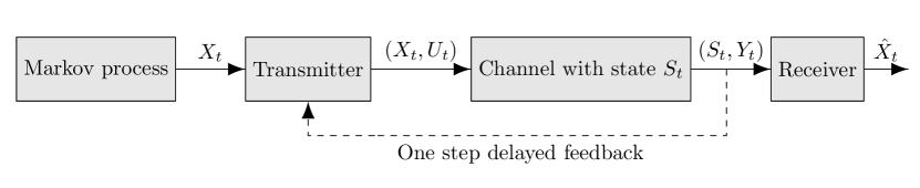
Figure 1: Remote estimation over channel with state.

Several variations of the above model have been considered in the literature. Models with noiseless communication channels have been considered in [1, 2, 3, 4, 5, 6]. Since the channel is noiseless, these papers assume that there are only two power levels: power level 0, which corresponds to not transmitting; and power level 1, which corresponds to transmitting. Under slightly different modeling assumptions, these papers identify the structure of optimal transmission and estimation strategies for first-order autoregressive sources with unimodal noise and for higher order autoregressive sources with orthogonal dynamics and isotropic Gaussian noise. It is shown that the optimal transmission strategy is threshold-based, i.e., the sensor transmits whenever the current error is greater than a threshold. It is also shown that the optimal estimation strategy is like Kalman filter: when the receiver receives a packet, the estimate is the received symbol; when it does not receive the packet, then the estimate is the one-step prediction based on the previous symbol. Quite surprisingly, these results show that there is no advantage in trying to extract information about the source realization from the choice of the power levels. The transmission strategy at the sensor is also called event-triggered communication because the sensor transmits when the event ‘error is greater than a threshold’ is triggered. Models with i.i.d. packet-drop channels are considered in [7, 8, 9], where it is assumed that the transmitter has two power levels: on or off. Remote estimation over additive noise channel is considered in [10].

In this paper we consider a remote estimation problem over packet-drop channel with Markovian state. We assume that the receiver observes the channel state and feeds it back to the transmitter with one step delay. Preliminary results for this model are presented in [11], where attention was restricted to a binary state channel with two input power values (ON or OFF). In the current paper, we consider arbitrary number of channel states and power levels. A related paper is [12], in which a remote estimation over packet-drop channels with Markovian state is considered. It is assumed that the sensor and the receiver know the channel state. It is shown that optimal estimation strategies are like Kalman filter. A detailed comparison with [12] is presented in Section V-A.

Several approaches for computing the optimal transmission strategies have been proposed in the literature. For noiseless channels, these include dynamic programing based approaches [4, 5, 13], approximate dynamic programming based approaches [14], renewal theory based approaches [15]. It is shown in [16] that for event-triggered scheduling, the posterior density follows a generalized closed skew normal (GCSN) distribution. For Markovian channels (when the state is not observed), a change of measure technique to evaluate the performance of an event-triggered scheme is presented in [17]. In this paper, we present a renewal theory based Monte Carlo approach for computing the optimal thresholds. A preliminary version of the results was presented in [9] for a channel with i.i.d. packet drops.

I-B Contributions

In this paper, we investigate team optimal transmission and estimation strategies for remote estimation over time varying packet-drop channels. We consider two models for the source: finite state Markov source and first order autoregressive source (over either integers or reals). Our main contributions are as follows.

1. For finite sources, we identify sufficient statistics for both the transmitter and the receiver and obtain a dynamic programming decomposition to compute optimal transmission and estimation strategies.

2. For autoregressive sources, we identify qualitative properties of optimal transmission and estimation strategies. In particular, we show that the optimal estimation strategy is like Kalman filter and the optimal transmission strategy only depends on the current source realization and the previous channel state (and does not depend on the receiver’s belief of the source). Furthermore, when the channel state is stochastically monotone (see Assumption 1 for definition), then for any value of the channel state, the optimal transmission strategy is symmetric and quasi-convex in the source realization. Consequently, when the power levels are finite, the optimal transmission strategy is threshold-based, where the thresholds only depend on the previous channel state.

3. We show that the above qualitative properties extend naturally to infinite horizon models.

4. For infinite horizon models, we present a Renewal Theory based Monte-Carlo algorithm to evaluate the performance of any threshold-based strategy. We then combine it with a simultaneous perturbation based stochastic approximation algorithm to provide an algorithm to compute the optimal thresholds. We illustrate our results with a numerical example of a remote estimation problem with a transmitter with two power levels and a Gilbert-Elliott erasure channel.

5. We show that the problem of transmitting over one of $m$ available i.i.d. packet-drop channels (at a constant power level) can be considered as special case of our model. We show that there exist thresholds $\{k^{(i)}_{t}\}_{i=1}^{m}$, such that it is optimal to transmit over channel $i$ if the error state $E_{t}\in[k^{(i)}_{t},k^{(i+1)}_{t})$. See Sec. V-C for details.

I-C Notation

We use uppercase letters to denote random variables (e.g, $X$, $Y$, etc), lowercase letters to denote their realizations (e.g., $x$, $y$, etc.). $\mathds{Z}$, $\mathds{Z}_{\geq 0}$ and $\mathds{Z}_{>0}$ denote respectively the sets of integers, of non-negative integers and of positive integers. Similarly, $\mathds{R}$, $\mathds{R}_{\geq 0}$ and $\mathds{R}_{>0}$ denote respectively the sets of reals, of non-negative reals and of positive reals. For any set $\mathbb{A}$, let $\mathds{1}_{\mathbb{A}}$ denote its indicator function, i.e., $\mathds{1}_{\mathbb{A}}(x)$ is $1$ if $x\in\mathbb{A}$, else $0$. $|\mathbb{A}|$ denotes the cardinality of set $\mathbb{A}$. $\Delta(\mathbb{X})$ denotes the space of probability distributions of $\mathbb{X}$. For any vector $v\in\mathds{R}^{n}$, $v_{i}\in\mathds{R}$ denotes the $i$-th component of $v$. For any vector $v$ and an interval $A=[a,b]$ of $\mathds{R}$, $w=[v]_{A}$ means that $w_{i}$ equals $a$ if $v_{i}\leq a$; equals $v_{i}$ if $v_{i}\in(a,b)$; and equals $b$ if $v_{i}\geq b$. Given a Borel subset $A\subseteq\mathds{R}$ and a density $\pi$, we use the notation $\pi(A)\coloneqq\int_{A}\pi(e)de$. For any vector $\mathbf{v}$, $\nabla_{\mathbf{v}}$ denotes the derivative with respect to $\mathbf{v}$.

I-D The communication system

We consider a remote estimation system shown in Fig. 1. The different components of the system are explained below.

I-D1 Source model

The source is a first-order time-homogeneous Markov chain $\{X_{t}\}_{t\geq 0}$, $X_{t}\in\mathbb{X}$. We consider two models for the source.

• Finite state Markov source. In this model, we assume that $\mathbb{X}$ is a finite set and denote the state transition matrix by $P$, i.e., for any $x,y\in\mathbb{X}$, $P_{xy}=\mathds{P}({X_{t+1}=y}\,|\allowbreak\,{X_{t}=x})$.

• First-order autoregressive source. In this model, we assume that $\mathbb{X}$ is either $\mathbb{Z}$ or $\mathbb{R}$. The initial state $X_{0}=0$ and for $t\geq 0$, the source evolves as

  $$X_{t+1}=aX_{t}+W_{t},$$ (1)

  where $a,W_{t}\in\mathbb{X}$ and $\{W_{t}\}_{t\geq 0}$ is an i.i.d. sequence where $W_{t}$ is distributed according to a symmetric and unimodal distribution $\mu$.

I-D2 Channel model

The channel is a packet-drop channel with state. The state process $\{S_{t}\}_{t\geq 0}\in\mathbb{S}$, is a first-order time-homogeneous Markov chain with transition probability matrix $Q$. We assume that $\mathbb{S}$ is finite. This is a standard model for time-varying wireless channels [18, 19].

The input alphabet of the channel is $\mathbb{X}$ and the output alphabet is $\mathbb{Y}\coloneqq\mathbb{X}\cup\{\mathfrak{E}\}$ where the symbols $\mathfrak{E}$ denotes that no packet was received. At time $t$, the channel output is denoted by $Y_{t}$.

The packet drop probability depends on the input power $U_{t}\in\mathbb{U}$, where $\mathbb{U}$ is the set of allowed power levels. We assume that $\mathbb{U}$ is a subset of $\mathds{R}_{\geq 0}$ and $\mathbb{U}$ is either a finite set of the form $\{0,u_{(1)},\dots,u_{\max}\}$ or an interval of the form $[0,u_{\max}]$, i.e., $\mathbb{U}$ is uncountable. When $U_{t}=0$, it means that the transmitter does not send a packet. In particular, for any realization $(x_{0:T},s_{0:T},u_{0:T},y_{0:T})$ of $(X_{0:T},S_{0:T},U_{0:T},Y_{0:T})$, we have

$$\mathds{P}(S_{t}=s_{t}\mid X_{0:t}=x_{0:t},S_{0:t-1}=s_{0:t-1},U_{0:t}=u_{0:t})\\ =\mathds{P}(S_{t}=s_{t}\mid S_{t-1}=s_{t-1})=Q_{s_{t-1}s_{t}},$$ (2)

and

$$\mathds{P}(Y_{t}=y_{t}\mid X_{0:t}=x_{0:t},S_{0:t}=s_{0:t},U_{0:t}=u_{0:t})\\ =\begin{cases}1-p(s_{t},u_{t}),&\mbox{if $y_{t}=x_{t}$}\\ p(s_{t},u_{t}),&\text{if $y_{t}=\mathfrak{E}$}\\ 0,&\mbox{otherwise},\end{cases}$$ (3)

where $p(s_{t},u_{t})$ is the probability that a packet transmitted with power level $u_{t}$ when the channel is in state $s_{t}$ is dropped. We assume that the set $\mathbb{S}$ of the channel states is an ordered set where a larger state means a better channel quality. Then, for all $s\in\mathbb{S}$, $p(s,u)$ is (weakly) decreasing in $u$ with $p(s,0)=1$ and $p(s,u_{\max})\geq 0$. Furthermore, we assume that for all $u\in\mathbb{U}$, $p(s,u)$ is decreasing in $s$.

I-E The decision makers and the information structure

There are two decision makers in the system—the transmitter and the receiver. At time $t$, the transmitter chooses the transmit power $U_{t}$ while the receiver chooses an estimate $\hat{X}_{t}\in\mathbb{X}$. Let $I^{1}_{t}$ and $I^{2}_{t}$ denote the information sets at the transmitter and the receiver respectively.

The transmitter observes the source realization $X_{t}$. In addition, there is one-step delayed feedback from the receiver to the transmitter. Thus, the information available at the transmitter is

$$I^{1}_{t}=\{X_{0:t},U_{0:t-1},S_{0:t-1},Y_{0:t-1}\}.$$

The transmitter chooses the transmit power $U_{t}$ according to

$$U_{t}=f_{t}(I^{1}_{t})=f_{t}(X_{0:t},U_{0:t-1},S_{0:t-1},Y_{0:t-1}),$$ (4)

where $f_{t}$ is called the transmission rule at time $t$. The collection $\bm{f}\coloneqq(f_{0},f_{1},\dots)$ for all time is called the transmission strategy.

The receiver observes $Y_{t}$ and, in addition, observes the channel state $S_{t}$. Thus, the information available at the receiver is

$$I^{2}_{t}=\{S_{0:t},Y_{0:t}\}.$$

The receiver chooses the estimate $\hat{X}_{t}$ is chosen according to

$$\hat{X}_{t}=g_{t}(I^{2}_{t})=g_{t}(S_{0:t},Y_{0:t}),$$ (5)

where $g_{t}$ is called the estimation rule at time $t$. The collection $\bm{g}\coloneqq(g_{0},g_{1},\dots)$ for all time is called the estimation strategy.

The collection $(\bm{f},\bm{g})$ is called a communication strategy.

I-F The performance measures and problem formulation

At each time $t$, the system incurs two costs: a transmission cost $\lambda(U_{t})$ and a distortion or estimation error $d(X_{t},\hat{X}_{t})$. Thus, the per-step cost is

$$c(X_{t},U_{t},\hat{X}_{t})=\lambda(U_{t})+d(X_{t},\hat{X}_{t}).$$

We assume that $\lambda(u)$ is (weakly) increasing in $u$ with $\lambda(0)=0$ and $\lambda(u_{\max})<\infty$. For the autoregressive source model, we assume that the distortion is given by $d({X_{t}-\hat{X}_{t}})$, where $d(\cdot)$ is even and quasi-convex with $d(0)=0$.

We are interested in the following optimization problems:

Problem 1 (Finite horizon).

In the model described above, identify a communication strategy $(\bm{f}^{*},\bm{g}^{*})$ that minimizes the total cost given by

$$J_{T}(\bm{f},\bm{g})\coloneqq\mathds{E}\bigg{[}\sum_{t=0}^{T-1}c(X_{t},U_{t},\hat{X}_{t})\bigg{]}.$$ (6)

Problem 2 (Infinite horizon).

In the model described above, given a discount factor $\beta\in(0,1]$, identify a communication strategy $(\bm{f}^{*},\bm{g}^{*})$ that minimizes the total cost given as follows:

1. For $\beta\in(0,1)$,

   $$J_{\beta}(\bm{f},\bm{g})=(1-\beta)\mathds{E}\bigg{[}\sum_{t=0}^{\infty}\beta^{t}c(X_{t},U_{t},\hat{X}_{t})\bigg{]}.$$ (7)

2. For $\beta=1$,

   $$J_{1}(\bm{f},\bm{g})=\lim_{T\to\infty}\frac{1}{T}\mathds{E}\bigg{[}\sum_{t=0}^{T-1}c(X_{t},U_{t},\hat{X}_{t})\bigg{]}.$$ (8)

Remark 1.

In the above model, it has been assumed that whenever the transmitter transmits (i.e., $U_{t}\neq 0$), it sends the source realization uncoded. This is without loss of generality because the channel input alphabet is the same as the source alphabet and the channel is symmetric. For such models, coding does not improve performance [20].

Problems 1 and 2 are decentralized stochastic control problems. The main conceptual difficulty in solving such problems is that the information available to the decision makers and hence the domain of their strategies grow with time, making the optimization problem combinatorial. One could circumvent this issue by identifying a suitable information state at the decision makers, which do not grow with time. In the following section, we discuss one such method to establish the structural results.

II Main results for finite state Markov sources

II-A Structure of optimal communication strategies

We establish two types of structural results. First, we use person-by-person approach to show that $(X_{0:t-1},U_{0:t-1})$ is irrelevant at the transmitter (Lemma 1); then, we use the common information approach of [21] and establish a belief-state for the common information $(S_{0:t},Y_{0:t})$ between the transmitter and the receiver (Theorem 1).

Lemma 1.

For any estimation strategy of the form (5), there is no loss of optimality in restricting attention to transmission strategies of the form

$$U_{t}=f_{t}(X_{t},S_{0:t-1},Y_{0:t-1}).$$ (9)

The proof proceeds by establishing that the process $\{X_{t},S_{0:t-1},Y_{0:t-1}\}_{t\geq 0}$ is a controlled Markov process controlled by $\{U_{t}\}_{t\geq 0}$. See Appendix A for details.

For any strategy $\bm{f}$ of the form (9) and any realization $(s_{0:T},y_{0:T})$ of $(S_{0:T},Y_{0:T})$, define $\varphi_{t}\colon\mathbb{X}\to\mathbb{U}$ as

$$\varphi_{t}(x)=f_{t}(x,s_{0:t-1},y_{0:t-1}),\quad\forall x\in\mathbb{X}.$$

Furthermore, define conditional probability measures $\pi^{1}_{t}$ and $\pi^{2}_{t}$ on $\mathbb{X}$ as follows: for any $x\in\mathbb{X}$,

$$\pi^{1}_{t}(x) \coloneqq\mathds{P}^{\bm{f}}(X_{t}=x\mid S_{0:t-1}=s_{0:t-1},Y_{0:t-1}=y_{0:t-1}),$$

$$\pi^{2}_{t}(x) \coloneqq\mathds{P}^{\bm{f}}(X_{t}=x\mid S_{0:t}=s_{0:t},Y_{0:t}=y_{0:t}).$$

We call $\pi^{1}_{t}$ the pre-transmission belief and $\pi^{2}$ the post-transmission belief. Note that when $(S_{0:T},Y_{0:T})$ are random variables, then $\pi^{1}_{t}$ and $\pi^{2}_{t}$ are also random variables (taking values in $\Delta(\mathbb{X})$), which we denote by $\Pi^{1}_{t}$ and $\Pi^{2}_{t}$.

For the ease of notation, define $B(\pi^{1},s,\varphi)$ as follows:

$$B(\pi^{1},s_{t},\varphi) \coloneqq\mathds{P}(Y_{t}=\mathfrak{E}\,|\,S_{0:t}=s_{0:t},Y_{0:t-1}=y_{0:t-1})$$

$$=\sum_{x_{t}\in\mathbb{X}}\pi^{1}(x_{t})p(s_{t},\varphi(x_{t})).$$ (10)

Furthermore, define $\pi^{1}|_{\varphi_{t},s}$ as follows:

$$\pi^{1}|_{\varphi,s}(x)\coloneqq\frac{\pi^{1}(x)p(s,\varphi(x))}{B(\pi^{1},s,\varphi)}.$$ (11)

Then, using Baye’s rule one can show the following:

Lemma 2.

Given any transmission strategy $\bm{f}$ of the form (9):

1. there exists a function $F^{1}$ such that

   $$\pi^{1}_{t+1}=F^{1}(\pi^{2}_{t})=\pi^{2}_{t}P.$$ (12)

2. there exists a function $F^{2}$ such that

   $$\pi^{2}_{t}=F^{2}(\pi^{1}_{t},s_{t},\varphi_{t},y_{t})=\begin{cases}\delta_{y_{t}},&\mbox{if $y_{t}\in\mathbb{X}$}\\ \pi^{1}_{t}|_{\varphi_{t},s_{t}},&\mbox{if $y_{t}=\mathfrak{E}$}.\end{cases}$$ (13)

Note that in (12), we are treating $\pi^{2}_{t}$ as a row-vector and in (13), $\delta_{y_{t}}$ denotes a Dirac measure centered at $y_{t}$. The update equations (12) and (13) are standard non-linear filtering equations. See supplementary material for proof.

Theorem 1.

In Problem 1 with finite state Markov source, we have that:

1. Structure of optimal strategies: There is no loss of optimality in restricting attention to transmission and estimation strategies of the form:

   $$U_{t} =f^{*}_{t}(X_{t},S_{t-1},\Pi^{1}_{t}),$$ (14)

   $$\hat{X}_{t} =g^{*}_{t}(\Pi^{2}_{t}).$$ (15)

2. Dynamic program: Let $\Delta(\mathbb{X})$ denote the space of probability distributions on $\mathbb{X}$. Define value functions $V^{1}_{t}\colon\Delta(\mathbb{X})\times\mathbb{S}\to\mathds{R}$ and $V^{2}_{t}\colon\Delta(\mathbb{X})\times\mathbb{S}\to\mathds{R}$ as follows: for any $s_{t}\in\mathbb{S}$,

   $$V^{1}_{T+1}(\pi^{1}_{t},s_{t})=0,$$ (16)

   and for $t\in\{T,\dots,0\}$

   $$V^{1}_{t}(\pi^{1}_{t},s_{t}) =\min_{\varphi_{t}\colon\mathbb{X}\to\mathbb{U}}\big{\{}\Lambda(\pi^{1}_{t},\varphi_{t})+H_{t}(x_{t},\pi^{1}_{t},s_{t},\varphi_{t})\big{\}},$$ (17)

   $$V^{2}_{t}(\pi^{2}_{t},s_{t}) =\min_{\hat{x}\in\mathbb{X}}D(\pi^{2}_{t},\hat{x})+V^{1}_{t+1}(\pi^{2}_{t}P,s_{t}),$$ (18)

   where

   $$\Lambda(\pi^{1},\varphi) \coloneqq\sum_{x\in\mathbb{X}}\lambda(\varphi(x))\pi^{1}(x),$$

   $$H_{t}(x,\pi^{1},s,\varphi) \coloneqq B(\pi^{1},s,\varphi)V^{2}_{t}(\delta_{x},s)$$

   $$\qquad+(1-B(\pi^{1},s,\varphi))V^{2}_{t}(\pi^{1}|_{\varphi,s},s),$$

   $$D(\pi^{2},\hat{x}) \coloneqq\sum_{x\in\mathbb{X}}d(x,\hat{x})\pi^{2}(x).$$

   Let $\Psi_{t}(s,\pi^{1})$ denote the arg min of the right hand side of (17) and $g^{*}_{t}(\pi^{2}_{t})\coloneqq\arg\min_{\hat{x}\in\mathbb{X}}D(\pi^{2},\hat{x})$. Then, the optimal transmission strategy is given by

   $$f^{*}_{t}(\cdot,s,\pi^{1}_{t})=\Psi_{t}(s,\pi^{1}_{t})$$

   and the optimal estimation strategy is given by $g^{*}_{t}$.

The proof follows from the common information approach [21]. See Appendix B for details.

Remark 2.

The first term in (17) is the expected communication cost, the second term is the expected cost-to-go. The first term in (18) is the expected distortion and the second term is the expected cost-to-go.

Remark 3.

In (17) we use $\min$ instead of $\inf$ for the following reasons. Let $\Phi$ denote the set of functions from $\mathbb{X}$ to $\mathbb{U}$, which is equal to $\prod_{x\in\mathbb{X}}\mathbb{U}$ (since $\mathbb{X}$ is finite). When $\mathbb{U}$ is finite, $\Phi$ is also finite and thus we can use $\min$ in (17). When $\mathbb{U}$ is uncountable, $\Phi$ is a product of compact sets and hence is compact and thus we can use $\min$ in (17).

Remark 4.

Note that the dynamic program in Theorem 1 is similar to a dynamic program for a partially observable Markov Decision Process (POMDP) with finite state space and finite or uncountable action space (see Remark 3). Thus, the dynamic program can be extended to infinite horizon discounted cost model after verifying standard assumptions. However, doing so does not provide any additional insight, so we do not present infinite horizon results for this model. We will do so for the autoregressive source model later in the paper, where we provide an algorithm to find the optimal time-homogeneous strategy for infinite horizon criteria.

III Main results for autoregressive sources

III-A Structure of optimal trategies for finite horizon model

We start with a change of variables. Define a process $\{Z_{t}\}_{t\geq 0}$ as follows: $Z_{0}=0$ and for $t\geq 0$,

$$Z_{t}=\begin{cases}aZ_{t-1},&\mbox{if $Y_{t}=\mathfrak{E}$}\\ Y_{t},&\mbox{if $Y_{t}\in\mathbb{X}$}.\end{cases}$$

Next, define processes $\{E_{t}\}_{t\geq 0}$, $\{E^{+}_{t}\}_{t\geq 0}$, which we call the error processes and $\{\hat{E}_{t}\}_{t\geq 0}$ as follows:

$$E_{t}\coloneqq X_{t}-aZ_{t-1},\quad E^{+}_{t}\coloneqq X_{t}-Z_{t},\quad\hat{E}_{t}\coloneqq\hat{X}_{t}-Z_{t}.$$

The processes $\{E_{t}\}_{t\geq 0}$ and $\{E^{+}_{t}\}_{t\geq 0}$ are related as follows: $E_{0}=0$, $E^{+}_{0}=0$, and for $t\geq 0$,

$$E^{+}_{t}=\begin{cases}E_{t},&\mbox{if $Y_{t}=\mathfrak{E}$}\\ 0,&\mbox{if $Y_{t}\in\mathbb{X}$}\end{cases}\quad\text{and}\quad E_{t+1}=aE^{+}_{t}+W_{t}.$$ (19)

The above dynamics may be rewritten as

$$E_{t+1}=\begin{cases}aE_{t}+W_{t},&\hbox{if $Y_{t}=\mathfrak{E}$}\\ W_{t},&\hbox{if $Y_{t}\neq\mathfrak{E}$}.\end{cases}$$ (20)

Since $X_{t}-\hat{X}_{t}=E^{+}_{t}-\hat{E}_{t}$, we have that $d(X_{t}-\hat{X}_{t})=d(E^{+}_{t}-\hat{E}_{t})$. Thus, with this change of variables, the per-step cost may be written as $\lambda(U_{t})+d(E^{+}_{t}-\hat{E}_{t})$.

Note that $Z_{t}$ is a deterministic function of $Y_{0:t}$. Hence, at time $t$, $Z_{t-1}$ is measurable at the transmitter and thus $E_{t}$ is measurable at the transmitter. Moreover, at time $t$, $Z_{t}$ is measurable at the receiver.

Lemma 3.

For any transmission and estimation strategies of the form (9) and (5), there exists an equivalent transmission and estimation strategy of the form:

$$U_{t} =\tilde{f}_{t}(E_{t},S_{0:t-1},Y_{0:t-1}),$$ (21)

$$\hat{X}_{t} =\tilde{g}_{t}(S_{0:t},Y_{0:t})+Z_{t}.$$ (22)

Moreover, for any transmission and estimation strategies of the form (21)–(22), there exist transmission and estimation strategies of the form (9) and (5) that are equivalent.

The proof is given in Appendix C.

An implication of Lemma 3 is that we may assume that the transmitter transmits $E_{t}$ and the receiver estimates

$$\hat{E}_{t}=\hat{X}_{t}-Z_{t}=\tilde{g}_{t}(S_{0:t},Y_{0:t}).$$

For this model, we can further simplify the structures of optimal transmitter and estimator as follows.

Theorem 2.

In Problem 1 with first-order autoregressive source, we have that:

1. Structure of optimal estimation strategy: At each time $t$, there is no loss of optimality in choosing the estimates $\{\hat{E}_{t}\}_{t\geq 0}$ as

   $$\hat{E}_{t}=0,$$

   or, equivalently, choosing the estimates $\{\hat{X}_{t}\}_{t\geq 0}$ as: $\hat{X}_{0}=0$, and for $t>0$,

   $$\hat{X}_{t}=\begin{cases}a\hat{X}_{t-1},&\mbox{if $Y_{t}=\mathfrak{E}$}\\ Y_{t},&\mbox{if $Y_{t}\in\mathds{R}$}\end{cases}$$ (23)

2. Structure of optimal transmission strategy: There is no loss of optimality in restricting attention to transmission strategies of the form

   $$U_{t}=\tilde{f}_{t}(E_{t},S_{t-1}).$$ (24)

3. Dynamic programming decomposition: Recursively define the following value functions: for any $e\in\mathds{R}$ and $s\in\mathbb{S}$,

   $$J_{T+1}(e,s) =0,$$ (25)

   and for $$t\in\{T,\dots,0\}$$,

   $$J_{t}(e,s) =\min_{u\in\mathbb{U}}\bar{H}_{t}(e,s,u),$$ (26)

   where

   $$\bar{H}_{t}(e,s,u)=\lambda(u)+\sum_{s^{\prime}\in\mathbb{S}}Q_{ss^{\prime}}p(s^{\prime},u)d(e)\\ +\mathds{E}[J_{t+1}(E_{t+1},S_{t})\,|\,E_{t}=e,S_{t-1}=s,U_{t}=u].$$

   Let $\tilde{f}^{*}_{t}(e,s)$ denote the arg min of the right hand side of (26). Then the transmission strategy $\bm{\tilde{f}^{*}}=(\tilde{f}^{*}_{0},\dots,\tilde{f}^{*}_{T})$ is optimal.

See Appendix D for the proof.

III-B Monotonicity and quasi-convexity of the optimal solution

For autoregressive sources we can establish monotonicity and quasi-convexity of the optimal solution. To that end, let us assume the following.

Assumption 1.

The channel transition matrix $Q$ is stochastic monotone, i.e., for all $i,j\in\{1,\dots,n\}$ such that $i>j$ and for any $\ell\in\{0,\dots,n-1\}$,

$$\sum_{k=\ell+1}^{n}Q_{ik}\geq\sum_{k=\ell+1}^{n}Q_{jk}.$$

Theorem 3.

For any $t\in\{0,\dots,T\}$, we have the following:

1. For all $s\in\mathbb{S}$, $J_{t}(e,s)$ is even and quasi-convex in $e$.

Furthermore, under Assumption 1,

1. For every $e\in\mathbb{X}$, $J_{t}(e,s)$ is decreasing in $s$.

2. For every $s\in\mathbb{S}$, the transmission strategy $\tilde{f}_{t}(e,s)$ is even and quasi-convex in $e$.

Sufficient conditions under which the value function and the optimal strategy are even and quasi-convex are identified in [22, Theorem 1]. Properties 1 and 3 follow because the above model satisfies these sufficient conditions. Property 2 follows from standard stochastic monotonicity arguments. The details are presented in the supplementary material.

An immediate consequence of Theorem 3 is the following:

Corollary 1.

Suppose that Assumption 1 is satisfied and $\mathbb{U}$ is finite set given by $\mathbb{U}=\{0,u^{(1)},\dots,u^{(m)}\}$. For any $i\in\{0,1,\dots,m\}$, define

$$k^{(i)}_{t}(s)\coloneqq\inf\{e\in\mathds{R}_{\geq 0}:\tilde{f}_{t}(e,s)=u^{(i)}\}.$$

For ease of notation, define $k^{(m+1)}_{t}(s)=\infty$.

Then, the optimal strategy is a threshold based strategy given as follows: for any $s\in\mathbb{S}$, $i\in\{0,\dots,m\}$ and $|e|\in\big{[}k^{(i)}_{t}(s),k^{(i+1)}_{t}(s)\big{)}$,

$$\tilde{f}_{t}(e,s)=u^{(i)}.$$ (27)

Some remarks

1. It can be shown that under the optimal strategy, $\Pi^{2}_{t}$ is symmetric and unimodal ($\mathrm{SU}$) (see Definition 1) around $\hat{X}_{t}$ and, therefore, $\Pi^{1}_{t}$ is $\mathrm{SU}$ around $a\hat{X}_{t-1}$. Thus, the transmission and estimation strategies in Theorem 2 depend on the pre- and post-transmission beliefs only through their means.

2. Since the distortion function is even and quasi-convex, we can write the threshold conditions

   $$k^{(i-1)}_{t}(s)\leq|e|<k^{(i)}_{t}(s)$$

   in (27) as

   $$d(k^{(i-1)}_{t}(s))\leq d(e)<d(k^{(i)}_{t}(s)).$$

   Thus, if we define distortion levels $D^{(i)}_{t}(s)=\big{[}d(k^{(i-1)}_{t}(s)),d(k^{(i)}_{t}(s))\big{)}$, then we can say that the optimal strategy is to transmit at power level $u_{(i)}$ if $E_{t}\in D^{(i)}_{t}(S_{t-1})$.

3. When $Y_{t}=\mathfrak{E}$, the update of the optimal estimate is same as the update equation of Kalman filter. For this reason, we refer to the estimation strategy (23) as a Kalman-filter like estimator.

III-C Generalization to infinite horizon model

Given a communication strategy $(\bm{f},\bm{g})$, let $D_{\beta}^{(f,g)}(e,s)$ and $P_{\beta}^{(f,g)}(e,s)$ denote respectively the expected distortion and expected transmitted prower when the system starts in state $(e,s)$, i.e., for $\beta\in(0,1)$,

$$D_{\beta}^{(f,g)}(e,s) \coloneqq(1-\beta)\mathds{E}^{(f,g)}\Big{[}\sum_{t=0}^{\infty}\beta^{t}d(E_{t})\,|\,E_{0}=e,S_{-1}=s\Big{]},$$

$$P_{\beta}^{(f,g)}(e,s) \coloneqq(1-\beta)\mathds{E}^{(f,g)}\Big{[}\sum_{t=0}^{\infty}\beta^{t}\lambda(U_{t})\,|\,E_{0}=e,S_{-1}=s\Big{]},$$

and for $\beta=1$,

$$D_{1}^{(f,g)}(e,s) \coloneqq\lim_{T\to\infty}\frac{1}{T}\mathds{E}^{(f,g)}\Big{[}\sum_{t=0}^{T-1}d(E_{t})\,|\,E_{0}=e,S_{0}=s\Big{]},$$

$$P_{1}^{(f,g)}(e,s) \coloneqq\lim_{T\to\infty}\frac{1}{T}\mathds{E}^{(f,g)}\Big{[}\sum_{t=0}^{T-1}\lambda(U_{t})\,|\,E_{0}=e,S_{0}=s\Big{]}.$$

Then, the performance of the strategy $(\bm{f},\bm{g})$ when the system starts in state $(e,s)$ is given by

$$J_{\beta}^{(f,g)}(e,s)\coloneqq D_{\beta}^{(f,g)}(e,s)+P_{\beta}^{(f,g)}(e,s).$$

The structure of optimal estimator, as established in Theorem 2, continues to hold for the infinite horizon setup as well. Thus, we can restrict attention to Kalman-filter like estimator given by (23) and look at the problem of finding the best response transmission strategy. This is a single agent stochastic control problem. If the per-step distortion is unbounded, then we need the following assumption—which implies that there exists a strategy whose performance is bounded—for the infinite horizon problem to be meaningful.

Assumption 2.

Let $f^{(0)}$ denote the transmission strategy that always transmits at power level $u_{\max}$ and $g^{*}$ denote the Kalman-filter like strategy given by (23). Then, for given $\beta\in(0,1]$, and for all $e\in\mathbb{X}$ and $s\in\mathbb{S}$, $D^{(f^{(0)},g)}_{\beta}(e,s)<\infty$.

Assumption 2 is always satisfied if $d(\cdot)$ is bounded. For $\beta=1$, $d(e)=e^{2}$ and $\mathbb{S}=\{0,1\}$, the condition $a^{2}(1-Q_{00})<1$ is sufficient for Assumption 2 to hold (see [23, Theorem 8] and [24, Corollary 12]). Similar sufficient conditions are given in [25, Theorem 1] for vector-valued Markov source processes with a Markovian packet-drop channel.

We now state the main theorem of this section.

Theorem 4.

In Problem 2 with first-order autoregressive processes under Assumption 2, we have that

1. Structure of optimal estimation strategy: The time-homogeneous strategy $\bm{\tilde{g}^{*}}=\{\tilde{g}^{*},\tilde{g}^{*},\dots\}$, where $\tilde{g}^{*}$ is given by (23), is optimal.

2. Structure of optimal transmission strategy: There is no loss of optimality in restricting attention to time-homogeneous transmission strategies of the form

   $$U_{t}=\tilde{f}_{\beta}(E_{t},S_{t-1}).$$

3. Dynamic programming decomposition: For $\beta\in(0,1)$, let $J_{\beta}$ be the smallest bounded solution of the following fixed point equation: for all $e\in\mathds{R}$ and $s\in\mathbb{S}$,

   $$J_{\beta}(e,s)=\min_{u\in\mathbb{U}}\bar{H}_{\beta}(e,s,u),$$ (28)

   where

   $$\bar{H}_{\beta}(e,s,u)=(1-\beta)\lambda(u)+\sum_{s^{\prime}\in\mathbb{S}}Q_{ss^{\prime}}p(s^{\prime},u)d(e)\\ +\beta\mathds{E}[J_{\beta}(E_{t+1},S_{t})\,|\,E_{t}=e,S_{t-1}=s,U_{t}=u].$$

   Let $\tilde{f}^{*}_{\beta}(e,s)$ denote the arg min of the right hand side of (28). Then the transmission $\bm{\tilde{f}^{*}_{\beta}}=(\tilde{f}^{*}_{\beta},\tilde{f}^{*}_{\beta},\dots)$ is optimal.

4. Results for $\beta=1$: Let $\tilde{f}^{*}_{1}$ be any limit point of $\{\tilde{f}^{*}_{\beta}\}_{\beta\in(0,1)}$ as $\beta\uparrow 1$. Then, $\tilde{f}^{*}_{1}$ is optimal strategy for Problem 2 with $\beta=1$.

The proof is given in Appendix E.

Remark 5.

We are not asserting that the dynamic program (28) has a unique fixed point. To make such an assertion, we would need to check the sufficient conditions for Banach fixed point theorem. These conditions [26] are harder to check than the sufficient conditions (P1)–(P3) of Proposition 2 that we verify in Appendix E.

Corollary 2.

The monotonicity properties of Theorem 3 hold for the infinite horizon value function $J_{\beta}$ and transmission strategy $\tilde{f}_{\beta}$ as well.

An immediate consequence of Corollary 2 is the following:

Corollary 3.

Suppose that Assumption 1 is satisfied and $\mathbb{U}$ is finite set given by $\mathbb{U}=\{0,u^{(1)},\dots,u^{(m)}\}$. For any $i\in\{0,1,\dots,m\}$, define

$$k^{(i)}_{\beta}(s)\coloneqq\inf\{e\in\mathds{R}_{\geq 0}:\tilde{f}_{(}e,s)=u^{(i)}\}.$$

For ease of notation, define $k^{(m+1)}_{\beta}(s)=\infty$.

Then, the optimal strategy is a threshold based strategy given as follows: for any $s\in\mathbb{S}$, $i\in\{0,\dots,m\}$ and $|e|\in\big{[}k^{(i)}_{\beta}(s),k^{(i+1)}_{\beta}(s)\big{)}$,

$$\tilde{f}_{\beta}(e,s)=u^{(i)}.$$ (29)

IV Computing optimal thresholds for autoregressive sources with finite actions

Suppose the power levels are finite and given by

$$\mathbb{U}=\{0,u^{(1)},\dots,u^{(m)}\},\quad m\in\mathds{Z}_{>0},$$

with $u^{(i)}<u^{(i+1)}$ and $i\in\{0,1,\dots,m-1\}$. From Corollary 3, we know that the optimal strategy for Problem 2 is a time-homogeneous threshold-based strategy of the form (27). Let $\mathbf{k}$ denote the thresholds $\{k^{(i)}_{\beta}(s)\}$ and $f^{(\mathbf{k})}$ denote the strategy (29). In this section, we first derive formulas for computing the performance of a general threshold-based strategy $f^{(\mathbf{k})}_{\beta}$ of the form (27) and then propose a stochastic approximation based algorithm to identify the optimal thresholds.

It is conceptually simpler to work with a post-decision model where the pre-decision state is $E_{t}$ and the post-decision state is $E^{+}_{t}$ given by (19). The timeline of the various system variables is shown in Fig. 2. In this model, the per-step cost is given by $\lambda(U_{t})+d(E^{+}_{t})$.

Figure 2: Timeline for pre- and post-transmission error state.

IV-A Performance of an arbitrary threshold-based strategy

For $\beta\in(0,1]$, pick a reference channel state $s^{\circ}\in\mathbb{S}$. Given an arbitrary threshold-based strategy $f^{(\mathbf{k})}_{\beta}$, suppose the system starts in state $(E^{+}_{-1},S_{-1})=(0,s^{\circ})$ and follows strategy $f^{(\mathbf{k})}_{\beta}$. Then, the process $\{(E^{+}_{t},S_{t})\}_{t\geq 0}$ is a Markov process. Let $\tau^{(0)}=0$ and for $n\in\mathds{Z}_{>0}$ let

$$\tau^{(n)}\coloneqq\{t>\tau^{(n-1)}:(E^{+}_{t-1},S_{t-1})=(0,s^{\circ})\}$$

denote the stopping times when the Markov process $\{(E^{+}_{t},S_{t})\}_{t\geq 0}$ revisits $(0,s^{\circ})$. We say that the Markov process regenerates at times $\{\tau^{(n)}\}_{n\in\mathds{Z}_{\geq 0}}$ and refer to the interval $\{\tau^{(n)},\dots,\tau^{(n-1)}\}$ as the $n$-th regenerative cycle.

Define the following:

• $L^{(\mathbf{k})}_{\beta}$: the expected cost during a regenerative cycle, i.e.,

  $$L^{(\mathbf{k})}_{\beta}\coloneqq\mathds{E}\Big{[}\sum_{t=0}^{\tau^{(1)}-1}\!\!\beta^{t}(\lambda(U_{t})+d(E^{+}_{t}))\Bigm{|}\\ E^{+}_{-1}=0,S_{{-1}}=s^{\circ}\Big{]}.$$ (30)

• $M^{(\mathbf{k})}_{\beta}$: the expected time during a regenerative cycle, i.e.,

  $$M^{(\mathbf{k})}_{\beta}\coloneqq\mathds{E}\Big{[}\sum_{t=0}^{\tau^{(1)}-1}\beta^{t}\,\Bigm{|}\,E^{+}_{-1}=0,S_{-1}=s^{\circ}\Big{]}.$$ (31)

Using ideas from renewal theory, we have the following.

Theorem 5.

For any $\beta\in(0,1]$, the performance of threshold-based strategy $f^{(\mathbf{k})}_{\beta}$ is given by

$$C^{(\mathbf{k})}_{\beta}\coloneqq C_{\beta}(f^{(\mathbf{k})}_{\beta},g^{*})=\frac{L^{(\mathbf{k})}_{\beta}}{M^{(\mathbf{k})}_{\beta}}.$$ (32)

See Appendix F for the proof.

IV-B Necessary condition for optimality

In order to find the optimal threshold, we first observe the following.

Lemma 4.

For any $\beta\in(0,1]$, $L^{(\mathbf{k})}_{\beta}$ and $M^{(\mathbf{k})}_{\beta}$ are differentiable with respect to $\mathbf{k}$. Consequently, $C^{(\mathbf{k})}_{\beta}$ is also differentiable.

The proof of Lemma 4 follows from first principles using an argument similar to that in the supplementary material for [15].

Let $\nabla_{\mathbf{k}}L^{(\mathbf{k})}_{\beta}$, $\nabla_{\mathbf{k}}M^{(\mathbf{k})}_{\beta}$ and $\nabla_{\mathbf{k}}C^{(\mathbf{k})}_{\beta}$ denote the derivatives of $L^{(\mathbf{k})}_{\beta}$, $M^{(\mathbf{k})}_{\beta}$ and $C^{(\mathbf{k})}_{\beta}$ respectively. Then, a sufficient condition for optimality is the following.

Proposition 1.

A necessary condition for thresholds $\mathbf{k}^{*}$ to be optimal is that $N^{(\mathbf{k}^{*})}_{\beta}=0$, where

$$N^{(\mathbf{k}^{*})}_{\beta}\coloneqq M^{(\mathbf{k})}_{\beta}\nabla_{\mathbf{k}}L^{(\mathbf{k})}_{\beta}-L^{(\mathbf{k})}_{\beta}\nabla_{\mathbf{k}}M^{(\mathbf{k})}_{\beta}.$$

Proof:.

The result follows from observing that $\nabla_{\mathbf{k}}C^{(\mathbf{k})}_{\beta}=N^{(\mathbf{k})}_{\beta}/(M^{(\mathbf{k})}_{\beta})^{2}$.

Remark 6.

If $C^{(\mathbf{k})}_{\beta}$ is convex in $\mathbf{k}$, then the condition in Proposition 1 is also sufficient for optimality. Based on numerical calculations we have observed that $C^{(\mathbf{k})}_{\beta}$ is convex in $\mathbf{k}$ but we have not been able to prove it analytically.

IV-C Stochastic approximation algorithm to compute optimal thresholds

In this section we present an iterative algorithm based on simultaneous perturbation and renewal Monte Carlo (RMC) [9, 27] to compute the optimal thresholds. We present this algorithm under the following assumption.

Assumption 3.

There exists a $K\in\mathbb{X}_{\geq 0}$ such that for the optimal transmission strategy

$$k^{(m-1)}(s)\leq K,\quad\forall s\in\mathbb{S}.$$

Remark 7.

Assumption 3 is equivalent to stating that for each channel state $s$, there is a state $e^{*}(s)$ such that for all $e\geq e^{*}(s)$, the optimal transmission strategy transmits at the maximum power level $u_{\max}$ in state $(e,s)$. Assumption 3 is similar to the channel saturation assumption in [14, Assumption 1] and [12, Remark 5].

Under Assumption 3, there is no loss of optimality in restricting attention to threshold strategies in the set

$$\mathcal{K}\coloneqq\{\mathbf{k}:k^{(i)}(s)\leq K,\,\forall s\in\mathbb{S},i\in\{0,\dots,m-1\}\}.$$

The main idea behind RMC is as follows. Given a threshold $\mathbf{k}$, consider the following sample-path based unbiased estimators of $L^{(\mathbf{k})}_{\beta}$ and $M^{(\mathbf{k})}_{\beta}$:

$$\widehat{\mathsf{L}}^{(\mathbf{k})}_{\beta} \coloneqq\frac{1}{N}\sum_{n=0}^{N-1}\sum_{t=\tau^{(n)}}^{\tau^{(n+1)}-1}\beta^{t-\tau^{(n)}}\Big{[}\lambda(U_{t})+d(E^{+}_{t})\Big{]},$$ (33)

$$\widehat{\mathsf{M}}^{(\mathbf{k})}_{\beta} \coloneqq\frac{1}{N}\sum_{n=0}^{N-1}\sum_{t=\tau^{(n)}}^{\tau^{(n+1)}-1}\beta^{t-\tau^{(n)}},$$ (34)

where $N$ is a large non-negative integer.

Then, simultaneous perturbation based unbiased estimators of $\nabla_{\mathbf{k}}L^{(\mathbf{k})}_{\beta}$ and $\nabla_{\mathbf{k}}M^{(\mathbf{k})}_{\beta}$ are given by

$$\widehat{\nabla}\mathsf{L}^{(\mathbf{k})}_{\beta} =\delta(\widehat{\mathsf{L}}^{(\mathbf{k}+c\delta)}_{\beta}-\widehat{\mathsf{L}}^{(\mathbf{k}-c\delta)}_{\beta})/2c,$$ (35)

$$\widehat{\nabla}\mathsf{M}^{(\mathbf{k})}_{\beta} =\delta(\widehat{\mathsf{M}}^{(\mathbf{k}+c\delta)}_{\beta}-\widehat{\mathsf{M}}^{(\mathbf{k}-c\delta)}_{\beta})/2c,$$ (36)

where $\delta$ is an appropriately chosen random variable having the same dimension as $\mathbf{k}$ and $c$ is a small positive constant. Typically, all components of $\delta$ are chosen independetly as either $\mathrm{Rademacher}(\pm 1)$ [28, 29] or $\mathrm{Normal}(0,1)$ [30, 31].

If the estimates $(\widehat{\mathsf{L}}^{(\mathbf{k})}_{\beta},\widehat{\mathsf{M}}^{(\mathbf{k})}_{\beta})$ and $(\widehat{\nabla}\mathsf{L}^{(\mathbf{k})}_{\beta},\widehat{\nabla}\mathsf{M}^{(\mathbf{k})}_{\beta})$ are generated from from independent sample paths, then the unbiasedness and independence of these estimates imply that

$$\widehat{\mathsf{N}}^{(\mathbf{k})}_{\beta}\coloneqq\widehat{\mathsf{M}}^{(\mathbf{k})}_{\beta}\widehat{\nabla}\mathsf{L}^{(\mathbf{k})}_{\beta}-\widehat{\mathsf{L}}^{(\mathbf{k})}_{\beta}\widehat{\nabla}\mathsf{M}^{(\mathbf{k})}_{\beta}$$

is an unbiased estimator of $N^{(\mathbf{k})}_{\beta}$.

Then, the RMC algorithm to compute the optimal threshold is as follows.

1. Let $j=0$ and pick any initial guess $\mathbf{k}_{0}$.

2. For sufficiently large number of iterations do

   1. Generate $\widehat{\mathsf{L}}^{(\mathbf{k}_{j})}_{\beta}$ and $\widehat{\mathsf{M}}^{(\mathbf{k}_{j})}_{\beta}$ according to (33)–(34).

   2. Sample a random direction $\delta$.

   3. Generate $\widehat{\nabla}\mathsf{L}^{(\mathbf{k}_{j})}_{\beta}$ and $\widehat{\nabla}\mathsf{M}^{(\mathbf{k}_{j})}_{\beta}$ according to (35)–(36).

   4. Compute:

      $$\widehat{\mathsf{N}}^{(\mathbf{k}_{j})}_{\beta}\coloneqq\widehat{\mathsf{M}}^{(\mathbf{k}_{j})}_{\beta}\widehat{\nabla}\mathsf{L}^{(\mathbf{k}_{j})}_{\beta}-\widehat{\mathsf{L}}^{(\mathbf{k}_{j})}_{\beta}\widehat{\nabla}\mathsf{M}^{(\mathbf{k}_{j})}_{\beta}.$$

   5. Update:

      $$\mathbf{k}_{j+1}=[\mathbf{k}_{j}-\alpha_{j}\widehat{\mathsf{N}}^{(\mathbf{k}_{j})}_{\beta}]_{\mathcal{K}},$$

      where $[\cdot]_{\mathcal{K}}$ denotes projection on to the set $\mathcal{K}$ and $\{\alpha_{j}\}$ is a sequence of learning rates that satisfy $\sum_{j=1}^{\infty}\alpha_{j}=\infty$ and $\sum_{j=1}^{\infty}\alpha^{2}_{j}<\infty$.

   6. Set $j=j+1$.

We assume the following (which is a standard assumption for stochastic approximation algorithms, see e.g., [31, Assumption 5.6]).

Assumption 4.

The set of globally asymptotically stable equilibrium of the ODE

$$\frac{d\mathbf{k}}{dt}=-N{(\mathbf{k})}_{\beta}$$

is compact.

Theorem 6.

Consider the sequence of iterates $\{\mathbf{k}_{j}\}_{j\geq 0}$ obtained by the RMC algorithm described above. Let $\mathbf{k}^{*}$ be any limit point of $\{\mathbf{k}_{j}\}_{j\geq 0}$. Then, under Assumptions 3 and 4, $N^{(\mathbf{k}^{*})}_{\beta}=0$ and therefore $\nabla_{\mathbf{k}}C^{(\mathbf{k}^{*})}_{\beta}=0$.

Proof:.

The proof follows from [27, Corollary 1].

(a) $\lambda_{1}=100$

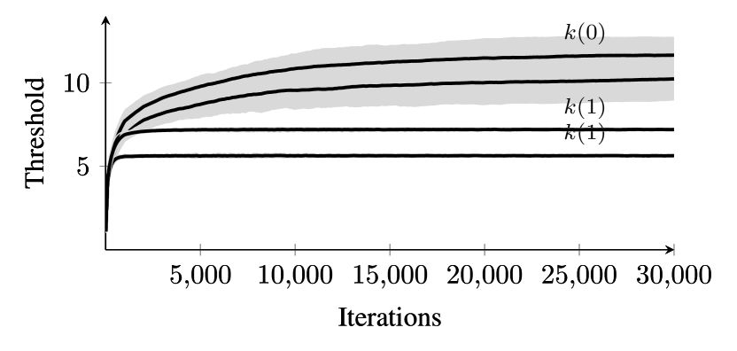
(b) $\lambda_{1}=200$

Figure 3: The thresholds versus iterations for different values of $\lambda_{1}$. The experiment is repeated 100 times. The bold lines represent the sample means and the shaded regions correspond to mean $\pm$ twice the standard deviation ($2\sigma$) across the runs.

IV-D Numerical example

Consider a real-valued autoregressive source with $a=1$, $\mu=\mathrm{Normal}(0,1)$ and a Gilbert-Elliott channel [32, 33] with state space $\mathbb{S}=\{0,1\}$, transition matrix $Q=\begin{bmatrix}0.3&0.7\\ 0.1&0.9\end{bmatrix}$, power levels $\mathbb{U}=\{0,1\}$, loss probability

$$p(0,0)=1,\quad p(0,1)=0.7,\quad p(1,0)=1,\quad p(1,1)=0.2,$$

transmission cost $\lambda(0)=0$, $\lambda(1)=\lambda_{1}$, and discount factor $\beta=0.9$. It can be verified that $Q$ is stochastic monotone. Thus, Assumption 1 is satisfied.

We run the RMC algorithm with $s^{\circ}=0$, $N=1000$, the learning rates $\{\alpha_{j}\}$ chosen according to ADAM [34] (with $\alpha$ parameter of ADAM equal to $0.1$ and other parameters taking their default values as stated in [34]), $\delta=\mathrm{Normal}(0,1)$ and $c=0.1$. Note that since $m=1$, $k^{(0)}(s)=0$, and we simply use $k(0)$ and $k(1)$ to denote $k^{(1)}(0)$ and $k^{(1)}(1)$.

We pick 10 uniformly spaced values of $\lambda_{1}$ in $[50,200]$ and run the RMC algorithm for 30,000 iterations. Since the output is stochastic, we repeat each experiment 100 times. We take the value of $\mathbf{k}$ at the end of each run and compute $C^{(\mathbf{k})}_{\beta}$ using $\widehat{\mathsf{C}}^{(\mathbf{k})}_{\beta}=\widehat{\mathsf{L}}^{(\mathbf{k})}_{\beta}/\widehat{\mathsf{M}}^{(\mathbf{k})}_{\beta}$, where we compute $\widehat{\mathsf{L}}^{(\mathbf{k})}_{\beta}$ and $\widehat{\mathsf{M}}^{(\mathbf{k})}_{\beta}$ by averaging over $N=10^{6}$ renewals. The value of $\mathbf{k}$ at the end of the run and $C^{(\mathbf{k})}_{\beta}$ are shown in Table I. The table also shows the two-standard deviation (denoted by $\sigma$) uncertainty on $\mathbf{k}$ and $C^{(\mathbf{k})}_{\beta}$.

A plot of $\mathbf{k}$ versus iterations for $\lambda_{1}\in\{100,200\}$ is shown in Fig. 3. This shows that the thresholds converge relatively quickly.

TABLE I: Optimal thresholds and performance for different values of communication cost for $\beta=0.9$

$\lambda_{1}$	$k(0)$	$k(1)$	$C^{(\mathbf{k})}_{\beta}$
	($\text{mean}\pm 2\sigma$)	($\text{mean}\pm 2\sigma$)	($\text{mean}\pm 2\sigma$)
$50$	$8.669$ p m 1.408	$4.465$ p m 0.061	$4.991$ p m 0.015
$66.67$	$9.438$ p m 1.592	$4.914$ p m 0.056	$5.440$ p m 0.009
$83.33$	$9.843$ p m 1.212	$5.290$ p m 0.061	$5.791$ p m 0.008
$100$	$10.235$ p m 1.259	$5.635$ p m 0.063	$6.087$ p m 0.009
$116.67$	$10.377$ p m 1.227	$5.943$ p m 0.063	$6.334$ p m 0.013
$133.33$	$10.821$ p m 1.053	$6.226$ p m 0.068	$6.557$ p m 0.010
$150$	$10.991$ p m 1.203	$6.492$ p m 0.065	$6.750$ p m 0.017
$166.67$	$11.238$ p m 1.105	$6.744$ p m 0.076	$6.911$ p m 0.008
$183.33$	$11.523$ p m 1.089	$6.975$ p m 0.080	$7.070$ p m 0.007
$200$	$11.660$ p m 1.056	$7.203$ p m 0.086	$7.198$ p m 0.014

V Discussions

V-A Comparison with the results of [12]

Remote estimation over a packet-drop channel with Markovian state was recently considered in [12]. In [12] it is assumed that the transmitter knows the current channel state. In contrast, in our model we assume that the receiver observes the channel state and sends it back to the transmitter. So, the transmitter has access to a one-step delayed channel state.

In [12], the authors pose the problem of identifying the optimal transmission and estimation strategies for infinite horizon average cost setup for vector-valued autoregressive sources. They identify the common information based dynamic program and identify technical conditions under which the dynamic program has a deterministic solution. The dynamic program in [12] may be viewed as the infinite horizon average cost equivalent of the finite horizon dynamic program in Theorem 1. They then show that when the source dynamics are orthogonal and the noise dynamics are isotropic, there is no loss of optimality in restricting attention to estimation strategies of the form (15) and transmission strategies of the form (14). In addition, for every $\pi\in\Delta(\mathbb{X})$ and $s\in\mathbb{S}$, $\zeta_{t}(\cdot)\coloneqq f_{t}(\cdot,s,\pi)$ is symmetric and quasi-convex. This structural property of the transmitter implies that when the power levels are finite, there exist thresholds $\{k^{i}_{t}(s,\pi)\}_{i=0}^{m-1}$ such that the optimal strategy is a threshold based strategy as follows: for any $s\in\mathbb{S}$, $\pi\in\Delta(\mathbb{X})$, $i\in\{0,\dots,m\}$ and $|e|\in[k^{(i)}_{t}(s,\pi),k^{(i+1)}_{t}(s,\pi))$,

$$f_{t}(e,s,\pi)=u^{(i)}.$$ (37)

In this paper, we follow a different approach. We investigate both finite Markov sources and first order autoregressive sources. For Markov sources, we first show that there is no loss of optimality in restricting attention to estimation strategies of the form (15) and transmission strategies of the form (14). For autoregressive sources, we show that the structure of the transmission strategies can be further simplified to (23) and (24). In addition for every $s\in\mathbb{S}$, $\varphi_{t}(\cdot)=\tilde{f}_{t}(\cdot,s)$ is symmetric and quasi-convex. This structural property of the transmitter implies that when the power levels are finite, there exist thresholds $\{k^{i}_{t}(s)\}_{i=0}^{m-1}$ auch that the optimal strategy is a threshold based strategy given by (27).

Once we restrict attention to estimation strategy of the form (23), the best response strategy at the transmitter is a centralized MDP. This allows us to establish the existence of optimal deterministic strategies for both discounted and average cost infinite horizon models without having to resort to the detailed technical argument presented in [12].

Note that in the threshold-based strategies (37) identified in [12], the thresholds depend on the belief state $\pi$, while in the threshold-based strategies (27) identified in this paper, the thresholds do not depend on $\pi$. We exploit this lack of dependence on $\pi$ to develop a renewal theory based method to compute the performance of a threshold based strategy. The algorithm proposed in this paper will not work for threshold strategies of the form (37) due to the dependence on $\pi$ (which is uncountable).

V-B Comparison with the results of [15]

A method for computing the optimal threshold for remote estimation over noiseless communication channel (i.e., no packet drop) is presented in [15]. That method relies on computing $L^{(\mathbf{k})}_{\beta}$ and $M^{(\mathbf{k})}_{\beta}$ by solving the balance equations (which are Fredholm integral equations of the second kind) for the truncated Markov chain. When the channel is a packet-drop channel, the kernel of the Fredholm integral equation is discontinuous. Moreover, when the channel has state, the integral equation is multi-dimensional. Solving such integral equations is computationally difficult. The simulation based methods presented in this paper circumvent these difficulties.

V-C The special case with i.i.d. packet-drop channels

Consider the case when the packet drops are i.i.d., which can be viewed as a Markov channel with a single state (i.e., $|\mathbb{S}|=1$). Thus we may drop the dependence on $s$ from the value function and the strategies. Furthermore, Assumption 1 is trivially satisfied. Thus the result of Theorem 3 simplifies to the following.

Corollary 4.

For Problem 1 with i.i.d. packet drops the value function $J_{t}(e)$ and the optimal transmission strategy $f_{t}(e)$ are even and quasi-convex.

The above result is same as [7, Theorem 1]. Furthermore, when the power levels are finite, the optimal transmission strategy is characterized by thresholds $(k^{(1)}_{t},\dots,k^{(m-1)}_{t})$. For infinite horizon models the thresholds are time-invariant.

In addition, the renewal relationships of Theorem 5 continues to hold. The stopping times $\{\tau^{(n)}\}_{n\geq 0}$ correspond to times of successful reception and the proposed renewal Monte-Carlo algorithm is similar in spirit to [9]. Note that the algorithm proposed in [9] uses simultaneous perturbation to find the minimum of $C^{(k)}_{\beta}$, where $C^{(k)}_{\beta}$ is evaluated using renewal relationships. The algorithm proposed in this paper is different and uses simultaneous perturbations to find the roots of $N^{(\mathbf{k})}_{\beta}$, which coincide with the roots of $\nabla_{\mathbf{k}}C^{(\mathbf{k})}_{\beta}$.

It is worth highlighting that when the power levels are finite, the model can also be interpreted as a remote estimator that has the option of transmitting (at a constant power level) over one of $m$ available i.i.d. packet-drop channels, as shown in Fig 4. For channel $i$, $i\in\{1,\dots,m\}$, the transmission cost is $\lambda(i)$ and the drop probability is $p(i)$. We assume that the channels are ordered such that $\lambda(1)\leq\dots\leq\lambda(m)$ and $p(1)\geq\dots\geq p(m)$. In addition, the sensor has the option of not transmitting, which is denoted by $i=0$. Note that $\lambda(0)=0$ and $p(0)=1$. As argued above, the optimal transmission strategy in this case is characterized by thresholds $(k^{(1)}_{t},\dots,k^{(m-1)}_{t})$ and the sensor transmits over channel $i$, where $i$ is such that $|e_{t}|\in[k^{(i)}_{t},k^{(i+1)}_{t})$ (and we assume that $k^{(0)}_{t}=0$ and $k^{(m)}_{t}=\infty$). The above result is similar in spirit to [35], which considers i.i.d. source and additive noise channels.

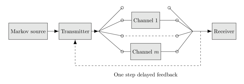
Figure 4: Remote estimation over multiple channels.

VI Conclusion

In this paper, we study remote estimation over a Markovian channel with feedback. We assume that the channel state is observed by the receiver and fed back to the transmitter with one unit delay. In addition, the transmitter gets ack/nack feedback for successful/unsuccessful transmission. Using ideas from team theory, we establish the structure of optimal transmission and estimation strategies for finite Markov sources and identify a dynamic program to determine optimal strategies with that structure. We then consider first-order autoregressive sources where the noise process has unimodal and symmetric distribution. Using ideas from majorization theory, we show that the optimal transmission strategy has a monotone structure and the optimal estimation strategy is like Kalman filter.

The structural results imply that threshold based transmitter is optimal when the power levels are finite. We provide a stochastic approximation based algorithm to compute the optimal thresholds and optimal performance. An example of a first-order autoregressive source model with Gilbert-Elliott channel is considered to illustrate the results.

Appendix A Proof of Lemma 1

Arbitrarily fix the estimation strategy $\bm{g}$ and consider the best response strategy at the transmitter. We will show that $\tilde{I}^{1}_{t}\coloneqq(X_{t},S_{0:t-1},Y_{0:t-1})$ is an information state at the transmitter. In particular, we will show that $\{\tilde{I}^{1}_{t}\}_{t\geq 1}$ satisfies the following properties:

$$\mathds{P}(\tilde{I}^{1}_{t+1}\,|\,I^{1}_{t},U_{t}) =\mathds{P}(\tilde{I}^{1}_{t+1}\,|\,\tilde{I}^{1}_{t},U_{t}),$$ (38)

and

$$\mathds{E}[c(X_{t},U_{t},\hat{X}_{t})\,|\,I^{1}_{t},U_{t}] =\mathds{E}[c(X_{t},U_{t},\hat{X}_{t})\,|\,\tilde{I}^{1}_{t},U_{t}].$$ (39)

Given any realization $(x_{0:T},s_{0:T},y_{0:T},u_{0:T})$ of the system variables $(X_{0:T},S_{0:T},Y_{0:T},U_{0:T})$, define $i^{1}_{t}=(x_{0:t},s_{0:t-1},y_{0:t-1},\allowbreak u_{0:t-1})$ and $\tilde{\imath}^{1}_{t}=(x_{t},s_{0:t-1},y_{0:t-1})$. Now, for any $\breve{\imath}^{1}_{t+1}=(x_{t+1},\breve{s}_{0:t},\breve{y}_{0:t})=(x_{t+1},\breve{s}_{t},\breve{y}_{t},\breve{\imath}^{1}_{t})$, we use the shorthand $\mathds{P}(\breve{\imath}^{1}_{t+1}|\tilde{\imath}^{1}_{0:t},u_{0:t})$ to denote $\mathds{P}(\tilde{I}^{1}_{t+1}=\breve{\imath}^{1}_{t+1}|\tilde{I}^{1}_{0:t}=\tilde{i}^{1}_{0:t},U_{0:t}=u_{0:t})$. Then,

$$\hskip-20.00003pt\mathds{P}(\breve{\imath}^{1}_{t+1}|i^{1}_{t},u_{t})=\mathds{P}(x_{t+1},\breve{s}_{t},\breve{y}_{t},\breve{\imath}^{1}_{t}|x_{0:t},s_{0:t-1},y_{0:t-1},u_{0:t})$$

$$\stackrel{{\scriptstyle(a)}}{{=}}\mathds{P}(x_{t+1}|x_{t})\mathds{P}(\breve{y}_{t}|x_{t},\breve{s}_{t})\mathds{P}(\breve{s}_{t}|s_{t-1})$$

$$\hskip 20.00003pt\times\mathds{1}{\{(\breve{s}_{0:t-1},\breve{y}_{0:t-1})=(s_{0:t-1},y_{0:t-1})\}}$$

$$=\mathds{P}(\breve{\imath}^{1}_{t+1}|x_{t},s_{0:t-1},y_{0:t-1},u_{t})$$

$$=\mathds{P}(\breve{\imath}^{1}_{t+1}|\tilde{\imath}^{1}_{t},u_{t})$$ (40)

where $(a)$ follows from the source and the channel models. This shows that (38) is true.

Now consider (39). Recall that $\hat{X}_{t}=g_{t}(I^{2}_{t})$. Therefore, the expectation in the left hand side of (39) depends on $\mathds{P}(I^{2}_{t}\,|\,I^{1}_{t},U_{t})$. By marginalizing (40) with respect to $X_{t+1}$, we get

$$\mathds{P}(I^{2}_{t}\,|\,I^{1}_{t},U_{t})=\mathds{P}(I^{2}_{t}\,|\,\tilde{I}^{1}_{t},U_{t}),$$

which implies (39).

Eq. (38) shows that $\{\tilde{I}^{1}_{t}\}_{t\geq 0}$ is a controlled Markov process controlled by $\{U_{t}\}_{t\geq 0}$. Eq. (39) shows that $\tilde{I}^{1}_{t}$ is sufficient for performance evaluation. Hence, by Markov decision theory [36], there is no loss of optimality in restricting attention to transmission strategies of the form (9).

Appendix B Proof of Theorem 1

Once we restrict attention to transmission strategies of the form (9), the information structure is partial history sharing [21]. Thus, one can use the common information approach of [21] and obtain the structure of optimal transmission strategy using this approach.

Following [21], we split the information available at each agent into a common information and local information. Common information is the information available to all decision makers in the future; the remaining data at the decision maker is the local information. Thus, at the transmitter, the common information is $C^{1}_{t}\coloneqq\{S_{0:t-1},Y_{0:t-1}\}$ and the local information is $L^{1}_{t}\coloneqq X_{t}$, and at the receiver, $C^{2}_{t}\coloneqq\{S_{0:t},Y_{0:t}\}$ and $L^{2}_{t}=\emptyset$. The state sufficient for input output mapping of the system is $(X_{t},S_{t})$. By [21, Proposition 1], we get that

$$\Theta^{1}_{t}(x,s)\coloneqq\mathds{P}(X_{t}=s,S_{t}=s|C^{1}_{t})$$

$$\Theta^{2}_{t}(x,s)\coloneqq\mathds{P}(X_{t}=s,S_{t}=s|C^{2}_{t})$$

are sufficient statistics for the common information at the transmitter and the receiver respectively. Now, we observe that

1. $\Theta^{1}_{t}$ is equivalent to $(\Pi^{1}_{t},S_{t-1})$ and $\Theta^{2}_{t}$ is equivalent to $(\Pi^{2}_{t},S_{t})$. This is because independence of $\{X_{t}\}_{t\geq 0}$ and $\{S_{t}\}_{t\geq 0}$ implies that $\theta^{1}_{t}(x,s)=\pi^{1}_{t}(x)Q_{s_{t-1}s}$ and $\theta^{2}_{t}(x,s)=\pi^{2}_{t}(x)\mathds{1}_{\{S_{t}=s\}}$.

2. The expected distortion $D(\Pi^{2}_{t},\hat{X}_{t})$ does not depend on $S_{t}$ and the evolution of $\Pi^{2}_{t}$ to $\Pi^{1}_{t+1}$ (given by Lemma 2) does not depend on $\hat{X}_{t}$.

Thus, from [21, Proposition 1] we get that the optimal strategy is given by the dynamic program of (17)–(18).

Appendix C Proof of Lemma 3

The proof relies on the fact that $Z_{t}$ is a deterministic function of $Y_{0:t}$, i.e., there exists an $\ell_{t}$ such that

$$Z_{t}=\ell_{t}(Y_{0:t}).$$

We prove the two parts separately. We use the notation $\bm{f}=(f_{1},\dots,f_{T})$, $\bm{g}=(g_{1},\dots,g_{T})$, $\bm{\tilde{f}}=(\tilde{f}_{1},\dots,\tilde{f}_{T})$ and $\bm{\tilde{g}}=(\tilde{g}_{1},\dots,\tilde{g}_{T})$.

1. Given a transmission and an estimation strategy $(\bm{f},\bm{g})$ of the form (9) and (5), define

   $$\tilde{f}_{t}(E_{t},S_{0:t-1},Y_{0:t-1})\\ =f_{t}(E_{t}+a\ell_{t-1}(Y_{0:t-1}),S_{0:t-1},Y_{0:t-1})$$

   and

   $$\tilde{g}_{t}(S_{0:t},Y_{0:t})=g_{t}(S_{0:t},Y_{0:t})-\ell_{t}(Y_{0:t}).$$

   Then, by construction the strategy $(\bm{\tilde{f}},\bm{\tilde{g}})$ is equivalent to $(\bm{f},\bm{g})$.

2. Given a transmission and an estimation strategy $(\bm{\tilde{f}},\bm{\tilde{g}})$ of the form (21)–(22), define

   $$f_{t}(X_{t},S_{0:t-1},Y_{0:t-1})\\ =\tilde{f}_{t}(X_{t}-a\ell_{t-1}(Y_{0:t-1}),S_{0:t-1},Y_{0:t-1})$$

   and

   $$g_{t}(S_{0:t},Y_{0:t})=\tilde{g}_{t}(S_{0:t},Y_{0:t})+\ell_{t}(Y_{0:t}).$$

   Then, by construction the strategy $(\bm{f},\bm{g})$ is equivalent to $(\bm{\tilde{f}},\bm{\tilde{g}})$.

Appendix D Proof of Theorem 2

D-A Sufficient statistic and dynamic program

Similar to the construction of a prescription for the finite state Markov sources, for any transmission strategy $\bm{\tilde{g}}$ of the form (21) and any realization $(s_{0:t-1},y_{0:t})$ of $(S_{0:t-1},Y_{0:t})$, define $\varphi:\mathds{R}\to\mathbb{U}$ as:

$$\varphi(e)=\tilde{f}_{t}(e,s_{0:t-1},y_{0:t-1}),\,\forall e\in\mathds{R}.$$

Next, redefine the pre- and post-transmission beliefs in terms of the error process. In particular, $\pi^{1}_{t}$ is the conditional pdf of $E_{t}$ given $(s_{0:t-1},y_{0:t-1})$ and $\pi^{2}_{t}$ is the conditional pdf of $E^{+}_{t}$ given $(s_{0:t},y_{0:t})$.

Let $R_{t}=\mathds{1}_{\{Y_{t}\in\mathbb{X}\}}$ and $r_{t}$ denote the realization of $R_{t}$. The time evolution of $\pi^{1}_{t}$ and $\pi^{2}_{t}$ is similar to Lemma 2. In particular, we have

Lemma 5.

Given any transmission strategy $\bm{f}$ of the form (4):

1. there exists a function $F^{1}$ such that

   $$\pi^{1}_{t+1}=F^{1}(\pi^{2}_{t})=\tilde{\pi}^{2}_{t}\star\mu,$$ (41)

   where $\tilde{\pi}^{2}_{t}$ given by $\tilde{\pi}^{2}_{t}(e)\coloneqq(1/|a|)\pi^{2}_{t}(e/a)$ is the conditional probability density of $aE^{+}_{t}$, $\mu$ is the probability density function of $W_{t}$ and $\star$ is the convolution operation.

2. There exists a function $F^{2}$ such that for any realization $r_{t}\in\{0,1\}$ of $R_{t}$

   $$\pi^{2}_{t}=F^{2}(\pi^{1}_{t},s_{t},\varphi_{t},r_{t}).$$

   In particular,

   $$\pi^{2}_{t}=F^{2}(\pi^{1}_{t},s_{t},\varphi_{t},r_{t})=\begin{cases}\pi^{1}_{t}|_{\varphi_{t},s_{t}},&\mbox{if $r_{t}=0$}\\ \delta_{0}&\mbox{if $r_{t}=1$}.\end{cases}$$ (42)

The dynamic program of Theorem 1 can be rewritten in terms of the error process as given below. Consider $\mathbb{X}=\mathds{R}$ (similar derivation holds for $\mathbb{X}=\mathds{Z}$).

$$V^{1}_{T+1}(\pi^{1}_{t},s_{t}) =0,$$

and for $$t\in\{T,\dots,0\}$$

$$V^{1}_{t}(\pi^{1}_{t},s_{t}) =\min_{\varphi_{t}\colon\mathbb{X}\to\mathbb{U}}\Big{\{}\Lambda(\pi^{1}_{t},\varphi_{t})+H_{t}(\pi^{1}_{t},s_{t},\varphi_{t})\Big{\}}$$ (43)

$$V^{2}_{t}(\pi^{2}_{t},s_{t}) =D(\pi^{2}_{t})+V^{1}_{t+1}(\pi^{2}_{t}P,s_{t}),$$ (44)

where,

$$\Lambda(\pi^{1}_{t},\varphi_{t}) \coloneqq\int_{\mathds{R}}\lambda(\varphi(e))\pi^{1}_{t}(e)de,$$

$$H_{t}(\pi^{1}_{t},s_{t},\varphi) \coloneqq B(\pi^{1}_{t},s_{t},\varphi_{t})V^{2}_{t}(\delta_{0},s_{t})+$$

$$\hskip 20.00003pt(1-B(\pi^{1}_{t},s_{t},\varphi_{t}))V^{2}_{t}(\pi^{1}|_{\varphi,s_{t}},s_{t}),$$

$$D(\pi^{2}_{t}) \coloneqq\min_{\hat{e}\in\mathbb{X}}\int_{\mathds{R}}d(e-\hat{e})\pi^{2}_{t}(e)de.$$

Note that due to the change of variables, the expression for the first term of $H_{t}$ does not depend on the transmitted symbol. Consequently, the expression for $V^{1}_{t}$ is simpler than that in Theorem 1.

Remark 8.

The common-information approach for decentralized stochastic control for finite state and finite action models was presented in [21]. In general, to extend the approach to Borel state and action spaces, one needs to impose a topology on the space of prescriptions and establish an appropriate “measurable selection theorem”. Such technical difficulties are not present in the dynamic program of (43)–(44) because the common information is finite and, therefore, all prescriptions are measurable.

To establish the results of Theorem 2, we show that the above dynamic program satisfies a monotonicity property with respect to the partial order based on majorization. We start with some mathematical preliminaries needed to present this argument.

D-B Mathematical preliminaries

Definition 1 (Symmetric and unimodal density).

A probability density function $\pi$ on reals is said to be symmetric and unimodal ($\mathrm{SU}$) around $c\in\mathds{R}$ if for any $x\in\mathds{R}$, $\pi(c-x)=\pi(c+x)$ and $\pi$ is non-decreasing in the interval $(-\infty,c]$ and non-increasing in the interval $[c,\infty)$.

Definition 2 (Symmetric and quasi-convex prescription).

Given $c\in\mathds{R}$, a prescription $\theta\colon\mathds{R}\to\mathbb{U}$ is symmetric and quasi-convex (denoted by $\mathrm{SQC}(c)$) if $\theta(e-c)$ is even and quasi-convex.

Now, we state some properties of symmetric and unimodal distributions.

Property 1.

If $\pi$ is $\mathrm{SU}(c)$, then

$$c\in\arg\min_{\hat{e}\in\mathds{R}}\int_{\mathds{R}}d(e-\hat{e})\pi(e)de.$$

Proof:.

For $c=0$, the above property is a special case of [4, Lemma 12]. The result for general $c$ follows from a change of variables.

Property 2.

If $\pi^{1}_{t}$ is $\mathrm{SU}(0)$ and $\varphi_{t}\in\mathrm{SQC}(0)$, then for any $r_{t}\in\{0,1\}$ and $s_{t}\in\mathbb{S}$, $F^{2}(\pi^{1}_{t},s_{t},\varphi_{t},r_{t})$ is $\mathrm{SU}(0)$.

Proof:.

We prove the result for each $r_{t}\in\{0,1\}$ separately. Recall the update of $\pi^{1}_{t}$ given by (42).

• For $r_{t}=0$ and a given $s_{t}\in\mathbb{S}$, we have that if $\varphi_{t}\in\mathrm{SQC}(0)$, then $p(s_{t},\varphi_{t}(e)$ is $\mathrm{SU}(0)$ since $p(s_{t},\cdot)$ is decreasing and $p(s_{t},\varphi_{t}(e))=p(s_{t},\varphi(-e))$. Then $\pi^{1}_{t}(e)p(s_{t},\varphi_{t}(e))$ is $\mathrm{SU}(0)$ since the product of two $\mathrm{SU}(0)$ functions is $\mathrm{SU}(0)$. Hence $\pi^{2}_{t}$ is $\mathrm{SU}(0)$.

• For $r_{t}=1$, $\pi^{2}_{t}=\delta_{0}$, which is $\mathrm{SU}(0)$.

Property 3.

If $\pi^{2}_{t}$ is $\mathrm{SU}(0)$, then $F^{1}(\pi^{2}_{t})$ is also $\mathrm{SU}(0)$.

Proof:.

Recall that $F^{1}$ is given by (41). The property follows from the fact that convolution of symmetric and unimodal distributions is symmetric and unimodal [4].

Definition 3 (Symmetric rearrangement (SR) of a set).

Let $\mathbb{A}$ be a measurable set of finite Lebesgue measure, its symmetric rearrangement $\mathbb{A}^{\sigma}$ is the open interval centered around origin whose Lebesgue measure is same as $\mathbb{A}$.

Definition 4 (Level sets of a function).

Given a function $\ell\colon\mathds{R}\to\mathds{R}_{\geq 0}$, its upper-level set at level $\rho$, $\rho\in\mathds{R}$, is $\{x\in\mathds{R}:\ell(x)>\rho\}$ and its lower-level set at level $\rho$ is $\{x\in\mathds{R}:\ell(x)<\rho\}$.

Definition 5 (SR of a function).

The symmetric decreasing rearrangement $\ell^{\sigma}_{\downarrow}$ of $\ell$ is a symmetric and decreasing function whose level sets are the same as $\ell$, i.e.,

$$\ell^{\sigma}_{\downarrow}(x)=\int_{\mathds{R}_{\geq 0}}\mathds{1}_{\{z\in\mathds{R}:\ell(z)>\rho\}^{\sigma}}(x)d\rho.$$

Similarly, the symmetric increasing rearrangement $\ell^{\sigma}_{\uparrow}$ of $\ell$ is a symmetric and increasing function whose level sets are the same as $\ell$, i.e.,

$$\ell^{\sigma}_{\uparrow}(x)=\int_{\mathds{R}_{\geq 0}}\mathds{1}_{\{z\in\mathds{R}:\ell(z)<\rho\}^{\sigma}}(x)d\rho.$$

Definition 6 (Majorization).

Given two probability density functions $\xi$ and $\pi$ over $\mathds{R}$, $\xi$ majorizes $\pi$, which is denoted by $\xi\succeq_{m}\pi$, if for all $\rho\geq 0$,

$$\int_{|x|\geq\rho}\xi^{\sigma}_{\downarrow}(x)dx\geq\int_{|x|\geq\rho}\pi^{\sigma}_{\downarrow}(x)dx.$$

Definition 7 (SU-majorization).

Given two probability density functions $\xi$ and $\pi$ over $\mathds{R}$, $\xi$ SU majorizes $\pi$, which we denote by $\xi\succeq_{a}\pi$, if $\xi$ is $\mathrm{SU}$ and $\xi$ majorizes $\pi$.

An immediate consequence of Definition 7 is the following:

Lemma 6.

For any non-negative $\mathrm{SQC}(c)$, function $g$, $c\in\mathds{R}$, and given two probability density functions $\xi$ and $\pi$ over $\mathds{R}$, such that $\xi\succeq_{a}\pi$ and $\xi$ is $\mathrm{SU}(c)$, we have that for any $A\subseteq\mathds{R}$,

$$\int_{A}g(x)\xi(x)dx\geq\int_{A}g(x)\pi(x)dx.$$

Property 4.

For any $\xi\succeq_{a}\pi$, $F^{1}(\xi)\succeq_{a}F^{1}(\pi)$.

This follows from [4, Lemma 10].

Recall the definition of $D(\pi^{2})$ given after (44).

Property 5.

If $\xi\succeq_{a}\pi$, then

$$D(\pi)\geq D(\pi^{\sigma}_{\downarrow})\geq D(\xi^{\sigma}_{\downarrow})=D(\xi).$$

Proof:.

The inequalities follow from [4, Lemma 11]. The last equality holds since $\xi$ is $\mathrm{SU}(0)$ and thus $\xi^{\sigma}_{\downarrow}=\xi$.

Lemma 7.

For any $c\in\mathds{R}$, densities $\pi$ and $\xi$ and a prescription $\varphi$, there exists a $\mathrm{SQC}(c)$ prescription $\theta$, $c\in\mathds{R}$, such that for any $u\in\mathbb{U}$

$$\pi(\{e\in\mathds{R}\,:\,\varphi(e)\leq u\})=\xi(\{e\in\mathds{R}\,:\,\theta(e)\leq u\}).$$

We denote such a $\theta$ by $\mathcal{T}^{(\pi,\xi)}_{c}\varphi$.

Proof:.

Let $\eta(u)\coloneqq\pi(\{e\in\mathds{R}\,:\,\varphi(e)\leq u\})$. We prove the construction separately for $\mathbb{X}=\mathds{R}$ and $\mathbb{X}=\mathds{Z}$. First, let us consider $\mathbb{X}=\mathds{R}$. Let $A(u)$ be a symmetric set centered around $c\in\mathds{R}$ such that $\xi(A(u))=\eta(u)$. By construction, $\eta(u)$ is increasing in $u$ and therefore so is $A(u)$. Define $\theta(e)$ such that $A(u)$ is the lower level set of $\theta(e)$. By construction, $\theta(e)$ is symmetric around $c$. Moreover, since $A(u)$ is convex, $\theta(e)$ is quasi-convex.

Now, let us consider $\mathbb{X}=\mathds{Z}$ and $c=0$. (The proof for general $c$ follows from a change of variables). Let $\mathbb{U}_{\varphi}$ denote the set $\{\varphi(e)\,:\,e\in\mathds{Z}\}$. Note that $\mathbb{U}_{\varphi}$ is a finite or a countable set which we will index by $\{u^{(i)}\,;\,i\in\mathds{Z}_{\geq 0}\}$. Define $k^{(i)}$ such that

$$\xi(A^{(i-1)})<\eta^{(i)}\leq\xi(A^{(i)}),$$

where $A^{(i-1)}\coloneqq\{-k^{(i-1)},\dots,k^{(i-1)}\}$ and $A^{(i)}\coloneqq\{-k^{(i)},\dots,k^{(i)}\}$.

Now, for any $u^{(i)}\in\mathbb{U}_{\varphi}$, let $\eta^{(i)}$ denote $\eta^{(i)}\coloneqq\pi(\{e\in\mathds{Z}\,:\,\varphi(e)\leq u^{(i)}\})$. Define $\delta^{(i)}\coloneqq(\eta^{(i)}-\xi(A^{(i)}))/2$. Define the prescription $\theta$ as follows

$$\theta(e)=\begin{cases}u^{(i-1)},&\mbox{if $|e|\in\big{(}k^{(i-1)},k^{(i)}\big{)}$}\\ u^{(i-1)}\text{ w.p. $\delta^{(i-1)}$},&\mbox{if $|e|=k^{(i)}$}\\ u^{(i)}\text{ w.p. $\delta^{(i)}$},&\mbox{if $|e|=k^{(i)}$}.\end{cases}$$

Then, by construction, $\theta$ is $\mathrm{SQC}(0)$ and $\xi(\{e\in\mathds{Z}\,:\,\theta(e)\leq u\})=\eta(u)$. This completes the proof.

Remark 9.

Suppose $\theta=\mathcal{T}^{(\pi,\xi)}_{c}\varphi$. Then the probability of using power level $u$ at pre-transmission belief $\pi$ and prescription $\varphi$ is the same as that at pre-transmission belief $\pi$ and prescription $\theta$. In particular, for all $u\in\mathbb{U}$,

$$\pi(\{e\in\mathbb{X}:\varphi(e)=u\})=\xi(\{e\in\mathbb{X}:\theta(e)=u\}).$$

Property 6.

For any density $\xi$, $\pi$, and prescription $\varphi$ let $\theta=\mathcal{T}^{(\pi,\xi)}_{c}\varphi$. Then, for any $s\in\mathbb{S}$,

1. $B(\xi,s,\theta)=B(\pi,s,\varphi)$.

2. $\Lambda(\pi,\varphi)=\Lambda(\xi,\theta)$.

The above results follow from the definitions of $B$ and $\Lambda$ and Remark 9. See supplementary material for a detailed proof.

Property 7.

For any $\xi\succeq_{a}\pi$, where $\xi$ is $\mathrm{SU}(c)$, and prescription $\varphi$, let $\theta=\mathcal{T}^{(\xi,\pi)}_{c}\varphi$. Then, for any $s\in\mathbb{S}$

$$\xi|_{\theta,s}\succeq_{a}\pi|_{\varphi,s}.$$ (45)

Consequently, for any $s\in\mathbb{S}$ and $r\in\{0,1\}$, we have

$$F^{2}(\xi,s,\theta,r)\succeq_{a}F^{2}(\pi,s,\varphi,r).$$ (46)

Proof:.

We prove the result for finite $\mathbb{U}=\{u^{(0},\dots,u^{(m)}\}$. The result for the case when $\mathbb{U}$ is an interval follows from a discretization argument.

For any $i\in\{0,\dots,m\}$, let $A^{(i)}=\{e\,:\,\theta(e)=u^{(i)}\}$ and $B^{(i)}=\{e:\varphi(e)=u^{(i)}\}$ and $\bar{A}^{(i)}=\bigcup_{j=0}^{i}A^{(i)}$ and $B^{(i)}=\bigcup_{j=0}^{i}B^{(i)}$.

Since $\theta$ is $\mathrm{SQC}(0)$, $\bar{A}^{(i)}$ is an interval (while $\bar{B}^{(i)}$ need not be an interval). Define $a^{(i)}=\xi(\bar{A}^{(i)})$ and $b^{(i)}=\pi(\bar{B}^{(i)})$. Also define $\xi^{(i)}$ as $\xi^{(i)}(e)=\xi(e)\mathds{1}_{\{e\in\bar{A}^{(i)}\}}/a^{(i)}$ and $\pi^{(i)}=\pi^{(i)}(e)=\pi(e)\mathds{1}_{\{e\in\bar{B}^{(i)}\}}/b^{(i)}$. Then, by[4, Lemma 8],

$$\xi^{(i)}\succeq_{a}\pi^{(i)},\quad\forall i\in\{0,\dots,m\}.$$ (47)

Fix an $s\in\mathbb{S}$. For ease of notation, define $p^{(i)}=p(s,u^{(i)})$. Then, we can write the following expression for $\xi\big{|}_{\theta,s}$

$$\xi \big{|}_{\theta,s}(e)=\frac{1}{B(\xi,s,\theta)}\xi(e)p(s,\theta(e))$$

$$=\frac{\xi(e)}{B(\xi,s,\theta)}\sum_{i=0}^{m}p^{(i)}\mathds{1}_{\{e\in A^{(i)}\}}$$

$$\stackrel{{\scriptstyle(a)}}{{=}}\frac{\xi(e)}{B(\xi,s,\theta)}\sum_{i=0}^{m-1}[p^{(i)}-p^{(i+1)}]\mathds{1}_{\{e\in\bar{A}^{(i)}\}}+p^{(m)}\mathds{1}_{\{e\in\bar{A}^{(m)}\}}$$

$$=\frac{1}{B(\xi,s,\theta)}\sum_{i=0}^{m-1}a^{(i)}[p^{(i)}-p^{(i+1)}]\xi^{(i)}+a^{(m)}p^{(m)}\xi^{(m)},$$ (48)

where $(a)$ uses the fact that $A^{(i)}=\bar{A}^{(i)}\setminus\bar{A}^{(i-1)}$. By a similar argument, we have

$$\pi\big{|}_{\varphi,s}(e)=\frac{1}{B(\pi,s,\varphi)}\sum_{i=0}^{m-1}b^{(i)}[p^{(i)}-p^{(i+1)}]\pi^{(i)}\\ +b^{(m)}p^{(m)}\pi^{(m)}.$$ (49)

Property 6 implies that $a^{(i)}=b^{(i)}$. The monotonicity of $p(s,u)$ implies that $p^{(i)}-p^{(i+1)}\geq 0$. Using this, and combining (48) and (49) with (47), we get (45). Eq. (46) follows from (13).

D-C Qualitative properties of the value function and optimal strategy

Lemma 8.

The value functions $V^{1}_{t}$ and $V^{2}_{t}$ of (43)–(44), satisfy the following property.

1. For any $i\in\{1,2\}$, $s\in\mathbb{S}$, $t\in\{0,\dots,T\}$, and pdfs $\xi^{i}$ and $\pi^{i}$ such that $\xi^{i}\succeq_{a}\pi^{i}$, we have that $V^{i}_{t}(\xi^{i},s)\leq V^{i}_{t}(\pi^{i},s)$.

Furthermore, the optimal strategy satisfies the following properties. For any $s\in\mathbb{S}$ and $t\in\{0,\dots,T\}$:

1. if $\pi^{1}_{t}$ is $\mathrm{SU}(c)$, then there exists a prescription $\varphi_{t}\in\mathrm{SQC}(c)$ that is optimal. In general, $\varphi_{t}$ depends on $\pi^{1}_{t}$.

2. if $\pi^{2}_{t}$ is $\mathrm{SU}(c)$, then the optimal estimate $\hat{E}_{t}$ is $c$.

Proof:.

We proceed by backward induction. $V^{i}_{T+1}(\pi^{1},s)$, $i\in\{1,2\}$ trivially satisfy (V1). This forms the basis of induction. Now assume that $V^{1}_{t+1}(s,\pi^{1})$ also satisfies (V1). For $\xi^{2}\succeq_{a}\pi^{2}$, we have that

$$V^{2}_{t}(\pi^{2},s) =D(\pi^{2})+V^{1}_{t+1}(F^{1}(\pi^{2}),s)$$

$$\stackrel{{\scriptstyle(a)}}{{\geq}}D(\xi^{2})+V^{1}_{t+1}(F^{1}(\xi^{2}),s)=V^{2}_{t}(\xi^{2},s),$$ (50)

where $(a)$ follows from Properties 4 and 5 and the induction hypothesis. Eq. (50) implies that $V^{2}_{t}$ also satisfies (V1). Now, we have

$$H_{t}(\pi^{1},s,\varphi)=B(\pi^{1},s,\varphi)V^{2}_{t}(\delta_{0},s)+$$

$$\hskip 80.00012pt(1-B(\pi^{1},s,\varphi))V^{2}_{t}(\pi^{1}|_{\varphi,s},s)$$

$$\stackrel{{\scriptstyle(a)}}{{\geq}}B(\xi^{1},s,\theta)V^{2}_{t}(\delta_{0},s)+(1-B(\xi^{1},s,\theta))V^{2}_{t}(\xi^{1}|_{\theta,s},s)$$

$$=H_{t}(\xi^{1},s,\theta),$$ (51)

where $(a)$ holds due to Properties 6 and 7 and (50). Then, we have from (43)

$$V^{1}_{t}(\pi^{1},s) =\min_{\varphi\colon\mathbb{X}\to\mathbb{U}}\Big{\{}\Lambda(\pi^{1},\varphi)+H_{t}(\pi^{1},s,\varphi)\Big{\}}$$

$$\stackrel{{\scriptstyle(b)}}{{\geq}}\min_{\theta\colon\mathbb{X}\to\mathbb{U}}\Big{\{}\Lambda(\xi^{1},\theta)+H_{t}(\xi^{1},s,\theta)\Big{\}}$$

$$=V^{1}_{t}(\xi^{1},s),$$ (52)

where $(b)$ holds due to Property 6 and (51) and since inequality is preserved in point-wise minimization. This completes the induction step.

In order to show (V2), note that $\pi^{1}_{t}\succeq_{a}\pi^{1}_{t}$ trivially. Let $\varphi_{t}$ be the optimal prescription at $\pi^{1}_{t}$. If $\varphi_{t}\in\mathrm{SQC}(c)$, then we are done. If not, define $\theta_{t}=\mathcal{T}^{(\pi^{1}_{t},\pi^{1}_{t})}_{c}\varphi_{t}$ where the transformation $\mathcal{T}^{(\pi^{1}_{t},\pi^{1}_{t})}_{c}$ is introduced in Lemma 7. Then, the argument in (52) (with $\xi^{1}$ replaced by $\pi^{1}$) also implies (V2). Furthermore, (V3) follows from Property 1.

D-D Proof of Theorem 2

Proof of Part 1

Properties 2 and 3 imply that for all $t$, $\Pi^{2}_{t}$ is $\mathrm{SU}(0)$. Therefore, by Property 1, the optimal estimate $\hat{E}_{t}=0$. Recall that $\hat{E}_{t}=\hat{X}_{t}-Z_{t}$. Thus, $\hat{X}_{t}=Z_{t}$. This proves the first part of Theorem 2.

Proof of Parts 2 and 3

Lemmas 1 and 3 imply that there is no loss of optimality in restricting attention to transmitters of the form

$$U_{t}=\tilde{g}_{t}(E_{t},Y_{0:t-1}).$$ (53)

Part 1 implies that there is no loss of optimality in restricting attention to estimation strategies of the form (23). So, we assume that the transmission and estimation strategies are of these forms.

Since the estimation strategy is fixed, Problem 1 reduces to a single agent optimization problem. $\{(E_{t},S_{t-1})\}_{t\geq 0}$ is an information state for this single agent optimization problem for the following reasons:

1. Eq. (20) implies that $\{E_{t}\}_{t\geq 0}$ is a controlled Markov process controlled by $R_{t}$. Moreover, for any realization $(e_{0:t},u_{0:t},s_{0:t-1})$ of $(E_{0:t},U_{0:t},S_{0:t-1})$, we have

   $$\mathds{P}(R_{t}=0|e_{0:t},u_{0:t},s_{0:t-1}) =\sum_{s^{\prime}\in\mathbb{S}}Q_{ss^{\prime}}p(s^{\prime},u)$$

   $$=\mathds{P}(R_{t}=0|u_{t},s_{t-1}).$$

   Combining the two we get that

   $$\mathds{P}(E_{t+1},S_{t}|e_{0:t},u_{0:t},s_{0:t-1})=\mathds{P}(E_{t+1},S_{t}|e_{t},u_{t},s_{t-1}).$$

2. Using (19), the conditional expected per step cost may be written as

   $$\hskip-20.00003pt\mathds{E}[\lambda(U_{t})+d(E^{+}_{t})|e_{0:t},u_{0:t},s_{0:t-1}]$$

   $$=\lambda(u_{t})+\mathds{E}[p(S_{t},u)d(e)|S_{t-1}=s].$$ (54)

Thus, the optimization problem at the transmitter is an MDP with information state $(E_{t},S_{t-1})$. Therefore, from Markov decision theory, there is no loss of optimality in restriction attention to Markov strategies of the form $f_{t}(E_{t},S_{t-1})$. The optimal strategies of this form are given by the dynamic program of Part 3.

Appendix E Proof of Theorem 4

E-A Proof of Part 1)

The structure of Theorem  2 holds the the infinite horizon setup as well. The main idea is to use forward induction to show that the optimal estimate for the error process, $\hat{E}_{t}=0$. The structure of optimal $\hat{X}_{t}$ is then derived by using the change of variable introduced in Section III-A.

E-B Some preliminary properties

We prove the following properties, which will be used to establish the existence of the solution to the dynamic program  (28). Note that the per-step cost $c(e,s,u)$ given in (2) can be rewritten as $c(e,s,u)\coloneqq(1-\beta)(\lambda(u)+\sum_{s_{t}\in\mathbb{S}}Q_{ss_{t}}p(s_{t},u)d(e))$.

Our model satisfies the following properties ([26, Assumtions 4.2.1,4.2.2]).

Proposition 2.

Under Assumption 2, for any $\lambda(\cdot)\geq 0$, the following conditions of [26] are satisfied:

1. The per-step cost $c(e,s,u)$ is lower semi-continuous, bounded from below and inf-compact on $\mathds{R}\times\{0,1\}$, i.e., for all $e,r\in\mathds{R}$, the set $\{u\in\mathbb{U}\,:\,c(e,s,u)\leq r\}$ is compact.

2. For every $u\in\{0,1\}$, the transition kernel from $(E_{t},S_{{t-1}})$ to $(E_{t+1},S_{t})$ is strongly continuous.

3. There exists a strategy for which the value function is finite.

Proof:.

(P1) is true because of the following reasons. The action set $\mathbb{U}=\mathbb{U}$ is either finite or uncountable and the per-step cost $c(\cdot,s,u)$ is continuous on $\mathds{R}$ (and hence lower semi-continuous), and is non-negative. Finally, when $\mathbb{U}$ is finite, all subsets of $\mathbb{U}$ are compact. When $\mathbb{U}$ is uncountable, all closed subsets of $\mathbb{U}$ are compact.

To check (P2), note the following fact ([26, Example C.6]).

Fact 1

Let $P$ be a stochastic kernel and suppose that there is a $\sigma$-finite measure $\phi$ on $\mathbb{X}$ such that, for every $y\in\mathbb{X}$, $\mathds{P}(\cdot|y)$ has a density $p(\cdot|y)$ with respect to $\phi$, that is,

$$P(B|y)=\int_{B}p(x|y)\phi(dx),\quad\forall B\in\mathcal{B}(\mathbb{X}),y\in\mathbb{X}.$$

If $p(x|\cdot)$ is continuous on $\mathbb{X}$ for every $x\in\mathbb{X}$, then $P$ is strongly continuous.

(P2) is true for the following reasons. Let $P$ denote the transition kernel from $(E_{t},S_{{t-1}})$ to $(E_{t+1},S_{t})$. Then for any Borel subset $B$ of $\mathcal{B}(\mathbb{X})$,

$$P(E_{t+1}\in B\,|\,E_{t}=e,S_{t-1}=s,U_{t}=u)\\ =(1-p(s,u))\int_{B}\mu(w)dw+p(s,u)\int_{B}\mu(w-ae)dw.$$

Then, according to Fact 1, $P$ is strongly continuous since the real line $\mathds{R}$ with Lebesgue measure $\phi(dx)=dx$ is $\sigma$-finite and since the density $\mu$ is continuous on $\mathds{R}$.

(P3) is true due to Assumption 2.

E-C Proofs of Parts 2) and 3)

For ease of exposition, we assume $\mathbb{X}=\mathds{R}$. Similar argument works for $\mathbb{X}=\mathds{Z}$. We fix the optimal estimator with the Kalman-filter like structure (23) and identify the best performing transmitter, which is a centralized optimization problem. For the discounted setup, one expects that the optimal solution is given by the fixed point of the dynamic program (28) (similar to (25)–(26)). However, it is not obvious that there exists a fixed point of (28) because the distortion $d(\cdot)$ is unbounded.

Define the operator $\mathcal{B}$ given as follows: for any given $s\in\mathbb{S}$ and function $v:\mathds{R}\times\mathbb{S}\rightarrow\mathds{R}$

$$[\mathcal{B}v](e,s) \coloneqq\min_{u\in\mathbb{U}}\mathds{E}[c(e,s,u)+v(E_{t+1},S_{t})$$

$$\hskip 80.00012pt\,|\,E_{t}=e,S_{t-1}=s].$$

Then (28) can be expressed in terms of the operator $\mathcal{B}$ as follows:

$$[\mathcal{B}J_{\beta}](e,s) \coloneqq\min_{u\in\mathbb{U}}\mathds{E}[c(e,s,u)+J_{\beta}(E_{t+1},S_{t})$$

$$\hskip 80.00012pt\,|\,E_{t}=e,S_{t-1}=s].$$

Then, the proof of Parts 2) and 3) of the theorem follows directly from [26]. In particular, we have the following proposition, where the first part follows from [26, Theorem 4.2.3] and the second part follows from [26, Lemma 4.2.8].

Proposition 3.

Under (P1)–(P3), there exist fixed point solutions $J_{\beta}$ of (28). Let $J^{*}_{\beta}:\mathbb{X}\rightarrow\mathds{R}$ denote the smallest such fixed point and $\tilde{f}^{*}_{\beta}(e,s)$ denote the argmin of the right hand side of (28) for $J_{\beta}=J^{*}_{\beta}$. Then,

1. $\tilde{f}^{*}_{\beta}$ is the optimal strategy for Problem 2 with $\beta\in(0,1)$.

2. Let $J^{(0)}_{\beta}=0$ and define $J^{(n+1)}_{\beta}\coloneqq\mathcal{B}J^{(n)}_{\beta}$. Then, $J^{*}_{\beta}=\lim_{n\rightarrow\infty}J^{(n)}_{\beta}$.

E-D Properties of the value function

We can apply the vanishing discount approach and show that the result for the long-term average cost is obtained as a limit of those in the discounted setup, as $\beta\uparrow 1$.

Our model satisfies the following conditions  [37, 26].

Proposition 4.

Under Assumption 2, for any $\lambda(\cdot)\geq 0$, the value function $J_{\beta}$, as given by (28), satisfies the following conditions of [37, 26]: for any $s\in\mathbb{S}$, and $\lambda\in\mathds{R}_{\geq 0}$,

1. there exists a reference state $e_{0}\in\mathbb{X}$ and a non-negative scalar $M_{s}$ such that $J^{*}_{\beta}(e_{0},s)<M_{s}$ for all $\beta\in(0,1)$.

2. Define $h_{\beta}(e,s)=(1-\beta)^{-1}[J_{\beta}(e,s)-J_{\beta}(e_{0},s)]$. There exists a function $K_{s}:\mathbb{X}\to\mathds{R}$ such that $h_{\beta}(e,s)\leq K_{s}(e)$ for all $e\in\mathbb{X}$ and $\beta\in(0,1)$.

3. There exists a non-negative (finite) constant $L_{\lambda}$ such that $-L_{s}\leq h_{\beta}(e,s)$ for all $e\in\mathbb{X}$ and $\beta\in(0,1)$.

Therefore, if $\tilde{f}^{*}_{\beta}$ denotes an optimal strategy for $\beta\in(0,1)$, and $\tilde{f}^{*}_{1}$ is any limit point of $\{\tilde{f}^{*}_{\beta}\}$, then $\tilde{f}^{*}_{1}$ is optimal for $\beta=1$.

Proof:.

We prove the proposition for $\mathbb{X}=\mathds{R}$. Similar argument holds for $\mathbb{X}=\mathds{Z}$.

Let $\tilde{J}^{(0)}_{\beta}(e,s)$ denote the value function of the ‘always transmit with maximum power’ strategy. According to Assumption 2, $M_{s}=\tilde{J}^{(0)}_{\beta}(0,s)<\infty$. Hence, (S1) is satisfied with $e_{0}=0$ and $M_{s}=\tilde{J}^{(0)}_{\beta}(0,s)$.

Since not transmitting is optimal at state 0 (because the transmission strategy is $\mathrm{SQC}$ about 0), we have

$$J^{*}_{\beta}(0,s) =\beta\sum_{s_{t}\in\mathbb{S}}Q_{ss_{t}}\int_{\mathds{R}}\mu(w)J^{*}_{\beta}(w,s_{t})dw.$$

Let $\tilde{J}^{(1)}_{\beta}(e,s)$ denote the value function of the strategy that transmits with power level $u=\varphi(e)$ at time 0 and follows the optimal strategy from then on. Then

$$\tilde{J}^{(1)}_{\beta}(e,s)=(1-\beta)[\lambda(\varphi(e))+\sum_{s_{t}\in\mathbb{S}}Q_{ss_{t}}p(s_{t},\varphi(e))d(e)]$$

$$\hskip 60.00009pt+\beta\sum_{s_{t}\in\mathbb{S}}Q_{ss_{t}}\int_{\mathds{R}}\mu(w)J^{*}_{\beta}(w,s_{t})dw$$

$$=(1-\beta)[\lambda(\varphi(e))+\sum_{s_{t}\in\mathbb{S}}Q_{ss_{t}}p(s_{t},\varphi(e))d(e)]$$

$$\hskip 160.00024pt+J^{*}_{\beta}(0,s).$$ (55)

Since $J^{*}_{\beta}(e,s)\leq\tilde{J}^{(1)}_{\beta}(e,s)$ and $J^{*}_{\beta}(0,s)\geq 0$, from (55) we get that $(1-\beta)^{-1}[J^{*}_{\beta}(e,s)-J^{*}_{\beta}(0,s)]\leq\lambda(\varphi(e))+\sum_{s_{t}\in\mathbb{S}}Q_{ss_{t}}p(s_{t},\varphi(e))d(e)$. Hence (S2) is satisfied with $K_{s}(e)=\lambda(\varphi(e))+\sum_{s_{t}\in\mathbb{S}}Q_{ss_{t}}p(s_{t},\varphi(e))d(e)$.

According to [22, Theorem 1], the value function $J^{*}_{\beta}$ is even and quasi-convex and hence $J^{*}_{\beta}(e,s)\geq J^{*}_{\beta}(0,s)$. Hence (S3) is satisfied with $L_{s}=0$.

E-E Proof of Part 4)

The result for Part 4) of the theorem for $\mathbb{X}=\mathds{Z}$ follows from [37, Theorem 7.2.3] and for $\mathbb{X}=\mathds{R}$ the result of Part 4) follows from [26, Theorem 5.4.3].

Appendix F Proof of Theorem 5

For ease of notation, we use $\tau$ instead of $\tau^{(1)}$. Let $\mathcal{F}_{0}$ denote the event $\{E^{+}_{-1}=0,S_{-1}=s^{\circ}\}$ and $\mathcal{F}_{\tau}$ denote the event $\{E^{+}_{\tau-1}=0,S_{\tau-1}=s^{\circ}\}$.

First note that from (31) we can write

$$\mathds{E}[\beta^{\tau}\,|\,\mathcal{F}_{0}]=1-(1-\beta)M^{(\mathbf{k})}_{\beta}.$$ (56)

Now consider

$$C^{(\mathbf{k})}_{\beta} =(1-\beta)\mathds{E}\Big{[}\sum_{t=0}^{\infty}\beta^{t}(\lambda(U_{t})+d(E^{+}_{t}))\Bigm{|}\mathcal{F}_{0}\Big{]}$$

$$=(1-\beta)\mathds{E}\Big{[}\sum_{t=0}^{\tau-1}\beta^{t}(\lambda(U_{t})+d(E^{+}_{t}))\Bigm{|}\mathcal{F}_{0}\Big{]}$$

$$\quad+(1-\beta)\mathds{E}\Big{[}\beta^{\tau}\sum_{t=\tau}^{\infty}\beta^{t-\tau}(\lambda(U_{t})+d(E^{+}_{t}))\Bigm{|}\mathcal{F}_{0}\Big{]}$$

$$\stackrel{{\scriptstyle(a)}}{{=}}(1-\beta)L^{(\mathbf{k})}_{\beta}+(1-\beta)\mathds{E}[\beta^{\tau}\,|\,\mathcal{F}_{0}]$$

$$\quad\times\mathds{E}\Big{[}\sum_{t=\tau}^{\infty}\beta^{t-\tau}(\lambda(U_{t})+d(E^{+}_{t}))\Bigm{|}\mathcal{F}_{\tau}\Big{]}$$

$$\stackrel{{\scriptstyle(b)}}{{=}}(1-\beta)L^{(\mathbf{k})}_{\beta}+[1-(1-\beta)M^{(\mathbf{k})}_{\beta}]C^{(\mathbf{k})}_{\beta},$$ (57)

where the first term of $(a)$ uses the definition of $L^{(\mathbf{k})}_{\beta}$ as given by (30) and the second term of $(a)$ uses strong Markov property; $(b)$ uses (56) and time-homogenity. Rearranging terms in (57) we get (32).

Appendix G Proof of Lemma 2

Given any realization $(x_{0:T},s_{0:T},y_{0:T},u_{0:T})$ of the system variables $(X_{0:T},S_{0:T},Y_{0:T},U_{0:T})$, consider

$$\pi^{1}_{t+1}(x_{t+1}) =\mathds{P}(x_{t+1}|s_{0:t},y_{0:t})$$

$$=\sum_{x_{t}\in\mathbb{X}}\mathds{P}(x_{t+1}|x_{t})\mathds{P}(x_{t}|s_{0:t},y_{0:t})$$

$$=\sum_{x_{t}\in\mathbb{X}}P_{x_{t}x_{t+1}}\pi^{2}_{t}(x_{t})=\pi^{2}_{t}P$$ (58)

which is the expression for $F^{1}(\cdot)$.

For $F^{2}$, we consider the following two cases separately. First, given any realization $(x_{0:T},s_{0:T},y_{0:T},u_{0:T})$ of the system variables $(X_{0:T},S_{0:T},Y_{0:T},U_{0:T})$, consider

$$\pi^{2}_{t}(x)=\mathds{P}(X_{t}=x|s_{0:t},y_{0:t})$$ (59)

G-1 Case 1: $y_{t}\in\mathbb{X}$

For $y_{t}\in\mathbb{X}$, we have

(60)

G-2 Case 2: $y_{t}=\mathfrak{E}$

In this case we have

$$\pi^{2}_{t}(x) =\mathds{P}(X_{t}=x|s_{0:t},y_{0:t})$$

$$=\frac{\mathds{P}(X_{t}=x,Y_{t}=y_{t}|s_{0:t},y_{0:t-1})}{\mathds{P}(Y_{t}=y_{t}|s_{0:t},y_{0:t-1})}.$$ (61)

Now, consider the numerator of (61).

$$\mathds{P}(X_{t}=x_{t},Y_{t}=\mathfrak{E}\,|\,s_{0:t},y_{0:t-1})$$

$$\hskip 20.00003pt=\mathds{P}(Y_{t}=\mathfrak{E}\,|\,s_{0:t},y_{0:t-1},x_{t})\mathds{P}(x_{t}\,|\,s_{0:t},y_{0:t-1})$$

$$\hskip 20.00003pt\stackrel{{\scriptstyle(a)}}{{=}}\sum_{u\in\mathbb{U}}\mathds{1}_{\{\varphi_{t}(x_{t})=u\}}p(s_{t},\varphi_{t}(x_{t})))\pi^{1}_{t}(x_{t}),$$ (62)

where in $(a)$ we use (3) and the fact that $\mathds{P}(x_{t}\,|\,s_{0:t},y_{0:t-1})=\mathds{P}(x_{t}\,|\,s_{0:t-1},y_{0:t-1})$ because the channel state is independent of the source.

The denominator of (61) is obtained by averaging the numerator over $x_{t}\in\mathbb{X}$.

Appendix H Proof of Theorem 3

We first note that Assumption 1 implies the following.

Lemma 9.

[38] For any weakly increasing (respectively weakly decreasing) function $h^{\circ}$ we have

$$\mathds{E}[h^{\circ}(S_{t})\,|\,S_{t-1}=s]$$

is weakly increasing (respectively weakly decreasing) in $s$.

Proof: (Theorem 3, Parts 1) and 3)).

The results follow directly from [22, Theorem 1]. We verify conditions (C1)–(C5) of [22, Theorem 1] in Section H-A.

Remark 10.

Using similar argument as in finite horizon case, one can show that the for discounted case infinite horizon, with discount factor $\beta\in(0,1)$ and any $s\in\mathbb{S}$, the optimal value function $J^{*}_{\beta}(e,s)$ and the optimal rules $\tilde{f}^{*}_{\beta}(e,s)$ are even and quasi-convex in $e$.

Proof: (Theorem 3, Part 2)).

First we note that we can rewrite the right hand side of (26) as follows:

$$\bar{H}_{t}(e,s,u)\coloneqq\lambda(u)+\sum_{s_{t}\in\mathbb{S}}Q_{ss_{t}}[p(s_{t},u)d(e)+\bar{J}_{t}(e,s_{t},u)],$$

where $\bar{J}_{t}(e,s,u)\coloneqq\mathds{E}_{W}[J_{t+1}(aE_{t}+W_{t},s)\,|\,E_{t}=e,U_{t}=u]$.

We prove the result of Part 2) by backward induction. The statement is trivially true for $t=T+1$ as $J_{T+1}=0$. Assume that for all $e\in\mathbb{X}$, $J_{t+1}(e,s)$ is decreasing in $s$. Since $\bar{J}_{t}(e,s,u)$ is a weighted average of $J_{t+1}(E_{t+1},s)$ with non-negative weights, we have that for all $e\in\mathbb{X}$, $u\in\mathbb{U}$, $\bar{J}_{t}(e,s,u)$ is weakly decreasing in $s$. By assumption, $p(s,u)$ is also decreasing in $s$. Thus, for any $(e,u)$, $p(s,u)d(e)+\bar{J}_{t}(e,s)$ is decreasing in $s$. Thus by Lemma 9, for any $(e,s)$, $\bar{H}_{t}(e,s,u)$ is decreasing in $s$. Since the pointwise minimum of decreasing functions is decreasing, from (26) we have that $J_{t}(e,s)$ is decreasing in $s$. This completes the induction step.

H-A Verification of conditions (C1)–(C5) of [22, Theorem 2]

We prove the result for $\mathbb{X}=\mathds{R}$. Similar argument holds for $\mathbb{X}=\mathds{Z}$. To prove the result, we show that dynamic program (25)–(26) satisfies conditions (C1)–(C5) of [22, Theorem 1]. We use the notation $\mathrm{SQC}(0)$ for even and quasi-convex. To prove the lemma, we first define the following:

• The per-step cost function $c$ as follows: for any $e\in\mathds{R};s\in\mathbb{S}$ and $u\in\mathbb{U}$,

  $$c(e,s,u)\coloneqq\lambda(u)+\sum_{s_{t}\in\mathbb{S}}Q_{ss_{t}}p(s,u)d(e).$$ (63)

• Let $\tilde{p}(e^{+}\,|\,e,s;u)$ denote the conditional density of $E_{t}=e^{+}$ given $E_{t}=e$, $S_{t-1}=s$ and $U_{t}=u$.

• Let $A_{y}\coloneqq\{e^{+}\in\mathds{R}\,:\,e^{+}<y\}$.

• Define the function $M$ as follows: $M(y\,|\,e,s;u)\coloneqq 1-\int_{A_{y}}(\tilde{p}(e^{+}|e,s;u)+\tilde{p}(-e^{+}|e,s;u))de^{+}$.

For ease of reference, we restate the properties of the model:

1. $p(s,0)=1$ and $p(s,u_{\max})\geq 0$.

2. $\lambda(\cdot)$ is increasing with $\lambda(0)=0$.

3. $p(\cdot,\cdot)$ is decreasing in $s$ and $u$.

4. $d(\cdot)$ is even and quasi-convex with $d(0)=0$.

In addition, we impose the following assumptions on the probability density/mass function of the i.i.d. process $\{W_{t}\}_{t\geq 1}$:

1. The density $\mu$ of $W_{t}$ is even.

2. $\mu(\cdot)$ is unimodal (i.e., quasi-concave).

The following result follows from [22, Lemma 2].

Lemma 10.

Under (M4) and (M5), for any $e,y\in\mathbb{X}_{\geq 0}$, we have that

$$\mu(y-e)\geq\mu(y+e)$$

An immediate implication of Lemma 10 are the following.

Lemma 11.

Under (M4) and (M5), for any $a\in\mathbb{X}$ and $e,y\in\mathbb{X}_{\geq 0}$, we have that

$$a\big{[}\mu(y-ae)-\mu(y+ae)\big{]}\geq 0.$$

Proof:.

For $a\in\mathbb{X}_{\geq 0}$, from Lemma 10 we get that $\mu(y-ae)\geq\mu(y+ae)$. For $a\in\mathbb{X}_{<0}$, from Lemma 10 we get that $\mu(y+ae)\geq\mu(y-ae)$.

We now state and verify conditions (C1)–(C5) from [22, Theorem 2].

H-A1 Condition (C1)

For any $s\in\mathbb{S}$ and $u\in\mathbb{U}$, the per-step cost $c(e,s,u)$ is even and quasi-convex in $e$.

This follows from (63) and (M3).

H-A2 Condition (C2)

For any $s\in\mathbb{S}$ and $u\in\mathbb{U}$, $p(\cdot\,|\,\cdot,s;u)$ is even, i.e., for any $e^{+},e\in\mathds{R}$,

$$\tilde{p}(e^{+}\,|\,e,s;u)=\tilde{p}(-e^{+}\,|\,-e,s;u).$$ (64)

This follows from (M4).

H-A3 Condition (C3)

For any $s\in\mathbb{S}$, $u\in\mathbb{U}$ and $y\in\mathds{R}_{\geq 0}$, $M(y\,|\,e,s;u)$ is (weakly) increasing in $e$ for all $e\in\mathds{R}_{\geq 0}$.

In order to do so, we arbitrarily fix $s\in\mathbb{S}$.

Consider any $y\in\mathds{R}_{\geq 0}$. Then,

$$M(y\,|\,e,s;u)$$

$$\hskip 20.00003pt=1-\sum_{s_{t}\in\mathbb{S}}Q_{ss_{t}}p(s_{t},u)$$

$$\hskip 20.00003pt\times\Big{[}\int_{-\infty}^{y}(\mu(e^{+}-ae)+\mu(e^{+}+ae))de^{+}\Big{]}$$

$$\hskip 20.00003pt-\sum_{s_{t}\in\mathbb{S}}Q_{ss_{t}}(1-p(s_{t},u))\Big{[}\int_{-\infty}^{y}(\mu(e^{+})+\mu(-e^{+}))de^{+}\Big{]}$$

$$\hskip 20.00003pt\stackrel{{\scriptstyle(a)}}{{=}}1-\sum_{s_{t}\in\mathbb{S}}Q_{ss_{t}}p(s_{t},u)[\mathcal{M}(y-ae)+\mathcal{M}(y+ae)]$$

$$\hskip 20.00003pt-\sum_{s_{t}\in\mathbb{S}}Q_{ss_{t}}(1-p(s_{t},u))2\mathcal{M}(y),$$ (65)

where $\mathcal{M}$ is the cumulative density function of $\mu$ and in equality $(a)$, we use the evenness of $\mu$. The following lemma shows that $M(y|e,s,u)$ is increasing in $e$ for all $e\in\mathds{R}_{\geq 0}$.

Lemma 12.

For any $y\in\mathds{R}_{\geq 0}$, $M(y|e,s,u)$ is increasing in $e$, $e\in\mathds{R}_{\geq 0}$.

Proof:.

Let $M_{e}(y|e,s;u)$ denote $\partial M/\partial e$. Then

$$M_{e}(y|e,s;u)=\sum_{s_{t}\in\mathbb{S}}Q_{ss_{t}}p(s,u)a\big{[}\mu(y-ae)-\mu(y+ae)\big{]}.$$

From (M0) and Lemma 11, we get that $M_{e}(y|e,s;u)\geq 0$ for any $e,y\in\mathds{R}_{\geq 0}$ and $u\in\mathbb{U}$. Thus, $M(y|e,s;u)$ is increasing in $e$.

Remark 11.

For $\mathbb{X}=\mathds{Z}$, one needs to replace the partial derivatives with finite differences. See [22] for the proof.

H-A4 Condition (C4)

For any $s\in\mathbb{S}$, $u_{1},u_{2}\in\mathbb{U}$, $u_{1}<u_{2}$, $c(e,s,u)$ is submodular in $(e,u)$ on $\mathds{R}_{\geq 0}\times\mathbb{U}$.

Consider $e_{1},e_{2}\in\mathds{R}_{\geq 0}$ such that $e_{1}\leq e_{2}$. Then,

$$\hskip-20.00003ptc(e_{1},s,u_{2})-c(e_{2},s,u_{2})$$

$$=\sum_{s_{t}\in\mathbb{S}}Q_{ss_{t}}p(s_{t},u_{2})(d(e_{1})-d(e_{2}))$$

$$\stackrel{{\scriptstyle(a)}}{{\geq}}\sum_{s_{t}\in\mathbb{S}}Q_{ss_{t}}p(s_{t},u_{1})(d(e_{1})-d(e_{2}))$$

$$=c(e_{1},s,u_{1})-c(e_{2},s,u_{1}),$$ (66)

where $(a)$ holds since $d(\cdot)$ is $\mathrm{SQC}(0)$, with $d(e)\geq 0$, for all $e\in\mathds{R}$ and $p(s_{t},\cdot)$ is decreasing. Eq. (66) implies that for any $s\in\mathbb{S}$, $c(e,s,u)$ is submodular in $(e,u)$ on $\mathds{R}_{\geq 0}\times\mathbb{U}$.

H-A5 Condition (C5)

For any $s\in\mathbb{S}$, $u\in\mathbb{U}$ and $y\in\mathds{R}_{\geq 0}$, $M(y\,|\,e,s;u)$ is submodular in $(e,u)$ on $\mathds{R}_{\geq 0}\times\mathbb{U}$.

It is shown in Lemma  12 that $M$ is increasing in $e$. Recall $M_{e}$ as introduced in the proof of Lemma 12. From (M2), $M_{e}(y|e,s;u)$ is decreasing in $u$. Thus, $M(y|e,s;u)$ is submodular in $(e,u)$ on $\mathds{R}_{\geq 0}\times\mathbb{U}$.

Appendix I Proof of Property 6

Consider uncountable $\mathbb{U}$ and $\mathbb{X}=\mathds{R}$. Similar derivation holds for finite $\mathbb{U}$ and $\mathbb{X}=\mathds{Z}$.

1. Recall from (10),

   $$B(\pi,s,\varphi) =\int_{\mathds{R}}\pi(e)p(s,\varphi(e))de$$

   $$=\int_{\mathbb{U}}\Big{[}\int_{\mathds{R}}\pi(e)\mathds{1}_{\{\varphi(e)=u\}}de\Big{]}p(s,u)du$$

   $$\stackrel{{\scriptstyle(a)}}{{=}}\int_{\mathbb{U}}\Big{[}\int_{\mathds{R}}\xi(e)\mathds{1}_{\{\theta(e)=u\}}de\Big{]}p(s,u)du$$

   $$=B(\xi,s,\theta),$$

   where $(a)$ holds by Remark 9.

2. Recall from Theorem 1,

   $$\Lambda(\pi,\varphi) =\int_{\mathds{R}}\lambda(\varphi(e))\pi(e)de$$

   $$=\int_{\mathbb{U}}\Big{[}\int_{\mathds{R}}\pi(e)\mathds{1}_{\{\varphi(e)=u\}}de\Big{]}\lambda(u)du$$

   $$\stackrel{{\scriptstyle(b)}}{{=}}\int_{\mathbb{U}}\Big{[}\int_{\mathds{R}}\xi(e)\mathds{1}_{\{\theta(e)=u\}}de\Big{]}\lambda(u)du$$

   $$=\Lambda(\xi,\theta),$$

   where $(b)$ holds by Remark 9.

References

- [1] Y. Xu and J. P. Hespanha, “Optimal communication logics in networked control systems,” in Proc. IEEE Conference on Decision and Control, 2004, pp. 3527–3532.
- [2] O. C. Imer and T. Başar, “Optimal estimation with limited measurements,” in Proc. IEEE Conference on Decision and Control and European Control Conference, 2005, pp. 1029–1034.
- [3] M. Rabi, G. Moustakides, and J. Baras, “Adaptive sampling for linear state estimation,” SIAM Journal on Control and Optimization, vol. 50, no. 2, pp. 672–702, 2012.
- [4] G. M. Lipsa and N. C. Martins, “Remote state estimation with communication costs for first-order LTI systems,” IEEE Trans. Autom. Control, vol. 56, no. 9, pp. 2013–2025, 2011.
- [5] A. Nayyar, T. Başar, D. Teneketzis, and V. V. Veeravalli, “Optimal strategies for communication and remote estimation with an energy harvesting sensor,” IEEE Trans. Autom. Control, vol. 58, no. 9, pp. 2246–2260, 2013.
- [6] A. Molin and S. Hirche, “Event-triggered state estimation: An iterative algorithm and optimality properties,” IEEE Trans. Autom. Control, vol. 62, no. 11, pp. 5939–5946, Nov 2017.
- [7] J. Chakravorty and A. Mahajan, “Remote state estimation with packet drop,” in Proc. of 6th IFAC Workshop on Distributed Estimation and Control in Networked Systems, Sep 2016, pp. 7–12.
- [8] G. M. Lipsa and N. C. Martins, “Optimal state estimation in the presence of communication costs and packet drops,” in 2009 47th Annual Allerton Conference on Communication, Control, and Computing (Allerton), Sept 2009, pp. 160–169.
- [9] J. Chakravorty, J. Subramanian, and A. Mahajan, “Stochastic approximation based methods for computing the optimal thresholds in remote-state estimation with packet drops,” in Proc. of IEEE American Control Conference, May 2017, pp. 462–467.
- [10] X. Gao, E. Akyol, and T. Başar, “Optimal communication scheduling and remote estimation over an additive noise channel,” Automatica, vol. 88, pp. 57–69, 2018.
- [11] J. Chakravorty and A. Mahajan, “Structure of optimal strategies for remote estimation over Gilbert-Elliott channel with feedback,” in Proc. of the IEEE International Symposium on Information Theory, Jun 2017, pp. 1272–1276.
- [12] X. Ren, J. Wu, K. H. Johansson, G. Shi, and L. Shi, “Infinite horizon optimal transmission power control for remote state estimation over fading channels,” IEEE Trans. Autom. Control, vol. 63, no. 1, pp. 85–100, Jan 2018.
- [13] A. Molin and S. Hirche, “An iterative algorithm for optimal event-triggered estimation,” in 4th IFAC Conference on Analysis and Design of Hybrid Systems (ADHS’12), 2012, pp. 64–69.
- [14] K. Gatsis, A. Ribeiro, and G. J. Pappas, “Optimal power management in wireless control systems,” IEEE Trans. Autom. Control, vol. 59, no. 6, pp. 1495–1510, June 2014.
- [15] J. Chakravorty and A. Mahajan, “Fundamental limits of remote estimation of autoregressive Markov processes under communication constraints,” IEEE Trans. Autom. Control, vol. 62, no. 3, pp. 1109–1124, March 2017.
- [16] L. He, J. Chen, and Y. Qi, “Event-based state estimation: Optimal algorithm with generalized closed skew normal distribution,” to appear in IEEE Transactions on Automatic Control, pp. 1–8, 2018.
- [17] W. Chen, J. Wang, D. Shi, and L. Shi, “Event-based state estimation of hidden Markov models through a Gilbert-Elliott channel,” IEEE Trans. Autom. Control, vol. 62, no. 7, pp. 3626–3633, July 2017.
- [18] A. J. Goldsmith and P. P. Varaiya, “Capacity, mutual information, and coding for finite-state Markov channels,” IEEE Trans. Inf. Theory, vol. 42, no. 3, pp. 868–886, May 1996.
- [19] S. Yang, A. Kavcic, and S. Tatikonda, “Feedback capacity of finite-state machine channels,” IEEE Trans. Inf. Theory, vol. 51, no. 3, pp. 799–810, March 2005.
- [20] J. C. Walrand and P. Varaiya, “Optimal causal coding-decoding problems,” IEEE Trans. Inf. Theory, vol. 29, no. 6, pp. 814–820, Nov. 1983.
- [21] A. Nayyar, A. Mahajan, and D. Teneketzis, “Decentralized stochastic control with partial history sharing: A common information approach,” IEEE Trans. Autom. Control, vol. 58, no. 7, pp. 1644–1658, jul 2013.
- [22] J. Chakravorty and A. Mahajan, “Sufficient conditions for the value function and optimal strategy to be even and quasi-convex,” to appear in IEEE Transactions on Automatic Control, 2019.
- [23] M. Huang and S. Dey, “Stability of Kalman filtering with Markovian packet losses,” Automatica, vol. 43, no. 4, pp. 598–607, 2007.
- [24] E. R. Rohr, D. Marelli, and M. Fu, “Kalman filtering with intermittent observations: On the boundedness of the expected error covariance,” IEEE Trans. Autom. Control, vol. 59, no. 10, pp. 2724–2738, Oct 2014.
- [25] J. Wu, G. Shi, B. D. O. Anderson, and K. H. Johansson, “Kalman filtering over Gilbert-Elliott channels: Stability conditions and critical curve,” IEEE Trans. Autom. Control, vol. 63, no. 4, pp. 1003–1017, April 2018.
- [26] O. H. Lerma and J. B. Lasserre, Discrete-time Markov control processes : basic optimality criteria. Springer, 1996.
- [27] J. Subramanian and A. Mahajan, “Renewal Monte Carlo: Renewal theory based reinforcement learning,” arXiv: 1804.01116, Apr. 2018.
- [28] J. C. Spall, “Multivariate stochastic approximation using a simultaneous perturbation gradient approximation,” IEEE Trans. Autom. Control, vol. 37, no. 3, pp. 332–341, Mar 1992.
- [29] J. L. Maryak and D. C. Chin, “Global random optimization by simultaneous perturbation stochastic approximation,” IEEE Trans. Autom. Control, vol. 53, no. 3, pp. 780–783, 2008.
- [30] V. Katkovnik and Y. Kulchitsky, “Convergence of a class of random search algorithms,” Automation and Remote Control, vol. 33, no. 8, pp. 1321–1326, 1972.
- [31] S. Bhatnagar, H. Prasad, and L. Prashanth, Stochastic Approximation Algorithms. London: Springer, 2013, pp. 17–28.
- [32] E. N. Gilbert, “Capacity of a burst-noise channel,” Bell System Technical Journal, vol. 39, no. 5, pp. 1253–1265, 1960.
- [33] E. O. Elliott, “Estimates of error rates for codes on burst-noise channels,” Bell System Technical Journal, vol. 42, no. 5, pp. 1977–1997, 1963.
- [34] D. P. Kingma and J. Ba, “Adam: A method for stochastic optimization,” arxiv: 1412.6980, Jan 2017.
- [35] X. Gao, E. Akyol, and T. Başar, “On remote estimation with multiple communication channels,” in Proc. American Control Conference, July 2016, pp. 5425–5430.
- [36] P. R. Kumar and P. Varaiya, Stochastic Systems: Estimation, Identification and Adaptive Control. NJ, USA: Prentice-Hall, Inc., 1986.
- [37] L. I. Sennott, Stochastic dynamic programming and the control of queueing systems. New York, NY, USA: Wiley, 1999.
- [38] M. Puterman, Markov decision processes: Discrete Stochastic Dynamic Programming. John Wiley and Sons, 1994.