1 Introduction

In this paper we demonstrate a computational method to solve the inverse scattering problem for a star-shaped, smooth, penetrable obstacle in 2D. Broadly speaking, inverse problems in physical systems are statistical inference problems restricted by an initial and/or boundary value problem for a partial differential equation. Consequently, inverse problems are difficult since the quantity to be inferred is defined in a function space, while data is finite and noisy. Stuart [1] studied conditions for the well-posedness of the Bayesian formulation of inverse problems. Recently, Christen [2] showed that that the Bayesian formulation of inverse problems is well posed under more general conditions. In either case, Bayesian inverse problems defined on function spaces have two main difficulties: the computationally efficient representation of the function to be estimated and the sampling of a posterior measure defined on an infinite-dimensional space. Although there are many theoretical approaches to overcome this issues [3, 4, 1], the development of competitive computational methods for inverse problems remains a very active research field.

We rely on classical computational geometry methods to deal with the issues of function representation and sampling. First, instead of posing the problem in an infinite dimensional setting, we approximate the support of each scatterer using a point cloud [5]. The rationale of our approach is that the direct problem has a finite rank property [6], i.e., the Frechet derivative of the mapping from scattering obstacle to near field is a compact operator, and its singular values have zero as a limit point [7]. Secondly, we use the Bayesian paradigm to model the joint conditional probability of the non-convex hull of the point cloud and the scatterer constant refractive index given measurements of the near field (in the remainder of this paper, we shall refer to this conditional probability as the posterior distribution). Of note, we use the non-convex hull of the point cloud as spline control points to evaluate, on a finer mesh, the volume potential arising in the integral equation formulation of the direct problem. Finally, in order to sample the arising posterior distribution, we construct a probability transition kernel based on moves that commute with affine transformations of space. This property, first introduced by Christen and Fox [8], implies that the performance of the Markov Chain Monte Carlo (MCMC) method is independent of the aspect ratio of anisotropic distributions.

The outline of the paper is as follows. In Section 2, we introduce the direct scattering problem and propose a numerical solution. Section 3 is devoted to the representation of the shape of an obstacle based on a point cloud. This representation uses the $\alpha$-shape algorithm and allows us to parameterize the obstacle shape with a parameter and a cloud of points. In Section 4, we present the Bayesian formulation of the inverse problem. The solution of the inverse problem is the posterior probability distribution. Thereby, an affine invariant MCMC method to sample the posterior distribution is designed. Numerical results and discussion are presented in Section 5. Finally, Section 6 summarizes our findings, pointing out limitations and possible generalizations of our inference method.

2 The direct scattering problem

In this Section we describe the direct scattering problem and propose a method for its numerical solution. We refer the reader to [7] for a more detailed discussion about the mathematical formulation of the scattering problem for a penetrable obstacle.

Let us assume that the scatterer $D\subset\mathbb{R}^{2}$ is bounded and penetrable. If the incident wave is a plane wave, the acoustic scattering problem can be cast as the following problem for the Helmholtz equation (see [7]),

$$\begin{split}\Delta u(\mathbf{x})+k^{2}(b(\mathbf{x})+1)u(\mathbf{x})&=0\quad\text{in}\quad\mathbb{R}^{2},\\ u(\mathbf{x})&=u^{i}(\mathbf{x})+u^{s}(\mathbf{x}),\\ \lim_{r\rightarrow\infty}r\left(\frac{\partial u^{s}(\mathbf{x})}{\partial r}-iku^{s}(\mathbf{x})\right)&=0,\end{split}$$ (1)

where $u$ is the total field, $u^{i}(\mathbf{x})=\text{e}^{ik\mathbf{x}\cdot d}$ is the incident field, $u^{s}(\mathbf{x})$ is the scattered field, $r=|\mathbf{x}|$, and $k$ is the wavenumber. The refractive index is assumed to be constant on $D$,

$$b(\mathbf{x})=\left\{\begin{array}[]{lcc}{\bf b},&\mathbf{x}\in D\\ \\ 0,&\mathbf{x}\in\mathbb{R}^{2}-D\end{array}\right.$$

for ${\bf b}\in\mathbb{R},$ ${\bf{b}\neq-1}$.

The Helmholtz equation is equivalent to the Lippmann-Schwinger equation

$$u(x)=u^{i}-k^{2}\int_{D}\Phi(k|x-y|)b(y)u(y)dy,$$ (2)

where

$$\Phi(r)=-\frac{i}{4}H_{0}^{(1)}(r)$$ (3)

and $H_{0}^{(1)}$ is the Hankel function of the first class of order zero.

2.1 Numerical solution of the direct scattering problem

In order to obtain an efficient solution of the forward model, we approximate the volume potential in equation (2) using a corrected trapezoidal rule. The correction coefficients are calculated in [9]. Taking the first correction coefficient $c_{1}$, we obtain a fourth order approximation

$$u_{j,h}=u_{j,h}^{i}-h^{2}k^{2}\sum_{l\in\mathbb{Z}_{N}^{2}}\Phi_{j-l,h}b_{l,h}u_{l,h}\hskip 8.53581pt+O(h^{4}),\hskip 5.69054ptj\in\mathbb{Z}_{N}^{2}$$ (4)

where $\mathbb{Z}_{N}^{2}=\{j\in\mathbb{Z}^{2}:0\leq j_{k}\leq N,k=1,2\}$,

$$\Phi_{j,h}=\left\{\begin{array}[]{lc}\Phi(k|j|h)&j\neq 0\\ \\ \Phi_{j,h}=\beta_{1}&j=0,\end{array}\right.$$

$\beta_{1}=-\frac{i}{4}+\frac{1}{2\pi}\left(\ln\left(\frac{hk}{2}\right)+\gamma+c_{1}\right)$, and $\gamma=0.5772156649015328606\ldots$ is Euler’s constant.

The discrete approximation of equation (2) can be written in matrix form

$$(K_{D,b}+I)u_{h}=u_{h}^{i}.$$ (5)

Note that $K_{D,b}$ is a sparse matrix that depends on the obstacle and the refractive index. Of note, we can readily index the entries where the matrix is different from zero using the definition of $b$. Thus, the matrix structure allows us to solve the system efficiently (5). In Figure 1, we compare computational times to solve the Lippmann-Schwinger equation numerically using equation (5) with the numerical solution of Vainikko [10]. It is apparent that the method introduced above is considerably faster than the method of Vainikko.

Figure 1: Comparison of computational times between (in seconds) the method of Vainikko (red) and the method propose (blue) for solving the Lippmann-Schwinger equation with the configuration depicted in Example 1 of Section 5.

3 Point cloud approximation of a scatterer

Given a point cloud in two or three dimensions, many methods of computational geometry are available to represent its boundary [11, 12, 13, 14, 15]. The structural simplicity of these representations allows efficient handling for geometric deformations and topology changes. The results of this paper are based on these ideas. In order to construct this representation, we use the $\alpha$-shape algorithm that computes the non-convex hull of a set of points in the plane. This algorithm produces a polygonal hull ($\alpha$-shape) that depends on the value of a real parameter (called $\alpha$). To obtain a smooth boundary, we interpolate on the points that define the $\alpha$-shape with a third order B-spline. B-splines are used due to its local stability properties on the control points, see Figure 3 (a), (b). Palafox et al. [16] introduced this procedure to estimate the boundary of a smooth sound obstacle from far field data. A detailed description of the algorithm is as follows:

Data: Let us $Q=\{p_{i}\}_{t=1}^{m}$ a set of $m$ points within the domain of the problem, $Q\subset G\subset\mathbb{{R}}^{2}$, and $\alpha$ a positive real number.

Output: A third order B-spline using the point cloud non-convex hull as control points.

Step 1. Compute the $\alpha$-shape of $Q$, denoted by $S_{\alpha}(Q)$, using the $\alpha$-shape algorithm [5].

Step 2. If $S_{\alpha}(Q)$ is a valid polygon (i.e non-empty, non-self-intersected and non-disconnected):
Compute $\Gamma_{Q,\alpha}$ interpolating the points that define the polygon $S_{\alpha}(Q)$ with a third-order B-spline.

Algorithm 1 Spline interpolation of the non-convex hull of a point cloud in 2D

Of note, the $\alpha$-shape algorithm uses the Delaunay triangulation with vertices Q to compute $S_{\alpha}(Q)$ (see Figure 2 (a)).

Figure 2: Part (a) shows the $\alpha$-shape (green), the interpolating spline (blue), $\Gamma_{Q,\alpha}$, with $\alpha=0.4$, and the correspondent Delaunay triangulation (grey). In part (b) shows $\Gamma_{Q,\alpha}$ for different values of $\alpha$.

The algorithm defined above accounts for a well defined mapping from $Q$ and parameter $\alpha$ to a boundary $\Gamma_{Q,\alpha}$. Indeed, the polygon $S_{\alpha}(Q)$, and thus the smooth boundary $\Gamma_{Q,\alpha}$, is uniquely determined by $Q$. The positive parameter $\alpha$ determines how non-convex the smooth boundary $\Gamma_{Q,\alpha}$ is (see Figure 2 (b)).

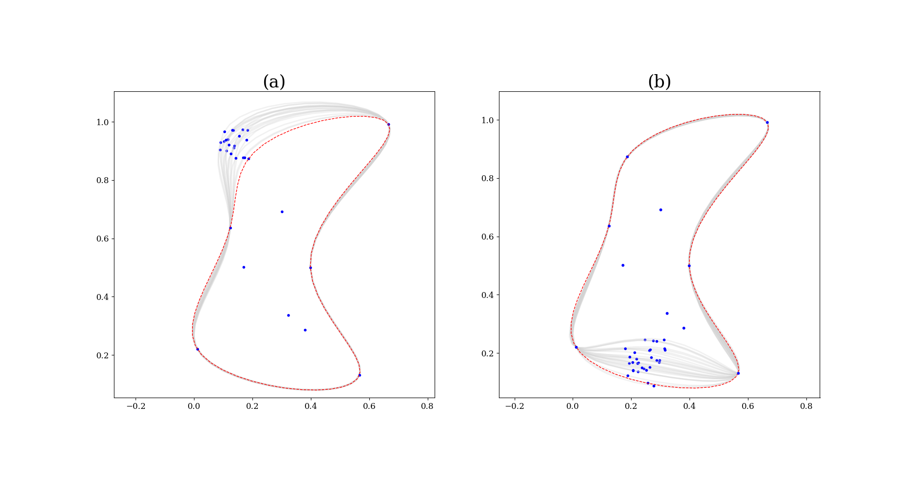
Figure 3: Part (a) shows the interpolating spline $\Gamma_{Q,\alpha}$, with $\alpha=0.5$, when a boundary point is perturbed, while part (b) shows the case when an interior point is perturbed. Local stability of the representation is apparent.

4 Bayesian Formulation of the Inverse Problem

In the inverse scattering problem, the task is to estimate the shape of the scatterer $D$ and the refractive index $\mathbf{b}$ given some available observations, e.g., near field data observed at some points of the domain $G$. The scattered field is obtained from several incoming plane waves with different directions $d$. We shall formulate the inverse problem in a finite dimensional space using the parametric representation of the obstacle described above. Thereby, the parameter space to be estimated is $\theta=(Q,\alpha,{\bf b})$.

We shall pose the inverse scattering problem using the Bayesian approach. This formulation allows us restating the inverse problem as “…a well-posed extension in a larger space of probability distributions…" [17]. The solution of the inverse problem is the posterior probability distribution.

Let us consider the following additive noise pointwise observation model:

$$\mathbf{d}_{j}:=u(x_{j})+\eta_{j},\quad j=1,\ldots,M.,$$ (6)

where $\{x_{j}\}_{j=1}^{M}$, is the set of points at which the scattered field is observed, $\eta_{x_{j}}\sim N(0,\sigma^{2})$ is additive noise, and $\mathbf{d}_{j}$ noisy observations. Concatenating all the observation, one can rewrite (6) as

$$\mathbf{d}:=F(\theta)+\eta$$ (7)

with $F:=[u(x_{1}),\ldots,u(x_{M})]$ denoting the mapping from the shape of $D$ (defined by Q and $\alpha$) and the refractive index $\mathbf{b}$ to the noise free observables, $\eta$ being normally distributed as $\mathcal{N}(0,\sigma^{2}I)$, and ${\bf d}=[\mathbf{d}_{1},\ldots,\mathbf{d}_{M}]^{T}$.

The Bayesian solution to our inverse problem is [17]

$$\pi(\theta|\mathbf{d})=\frac{L(\mathbf{d}|\theta)\pi(\theta)}{\pi(\mathbf{d})}.$$ (8)

where the likelihood is given by the noise distribution (7),

$$L(\mathbf{d}|\theta)=\left(2\pi\sigma\right)^{-M/2}\exp\left\{-\frac{1}{2}\sum_{x_{j}}\left|\left|\frac{\mathbf{d}_{j}-u(x_{j})}{\sigma}\right|\right|^{2}\right\}$$ (9)

assuming independent measurements. This function shows how measurements affect knowledge about $\theta$.

The prior distribution expresses the information about $\theta$ independent of the measurements $\mathbf{d}$. In our case, it is modeled as follows:

1. The refractive index ${\bf b}$, the point cloud $Q$ and the shape parameter $\alpha$ are taken as independent parameters; therefore

   $$\pi(\theta)=\pi(Q)\pi({\bf b})\pi(\alpha).$$

2. Uniform distributions for $Q$ and $\alpha$ are imposed, as a default selection. Consequently, the prior probabilities $\pi(Q)$, $\pi(\alpha)$ are constant on the domain $G$.

3. The choice of a gamma distribution for ${\bf b}$ is motivated by the application of the inverse scattering problem in elasticity imaging methods. The refractive index represents the Young modulus [18]. In this manner, the refractive index is assumed as a positive parameter.

   $${\bf b}\sim\text{Gamma}(\tilde{k},\tilde{\lambda}).$$ (10)

The resulting posterior distribution is explored using MCMC method with Metropolis Hastings (MH) by generating a Markov chain with equilibrium distribution (8). In the next Section we propose a the probability transition kernel to implement the MH algorithm.

4.1 An affine invariant probability transition kernel

By construction, the performance of the Metropolis-Hastings (MH) algorithm depends on a proposal probability distribution used to construct the probability transition kernel. Often, proposal probability distributions are gradient informed [4, 3]. However, there is a class of derivative-free proposals, first introduced by Christen and Fox [8], for arbitrary continuous distributions and requires no tuning, that gives rise to “…an algorithm that is invariant to scale, and approximately invariant to affine transformations of the state space…”. This property implies that the performance of the MCMC method is independent of the aspect ratio of anisotropic target distributions.

In Daza et al. [19], a MCMC method with the affine invariant property was used to approach the inverse scattering problem in an inhomogeneous medium with a convex obstacle. In this paper we build on previous results introducing an affine invariant proposal also for the $\alpha$ parameter of the non-convex hull of a point cloud. This proposal is defined from the circumradius of the Delaunay triangulation of the point cloud at the iteration t. The circumradius is used for two reasons: it contains information about the scale of the space and the $\alpha$-shape is obtained with decision criteria that involve the radius of the Delaunay triangulation (see details in [5]).

The probability transition kernel for the parameter space $\theta^{\left(t\right)}=\left(Q^{(t)},b^{\left(t\right)},\alpha^{\left(t\right)}\right)$, where $Q^{(t)}=\{p_{i}^{(t)}\}_{i=1}^{m}$ is given by

$$K(\theta^{\left(t\right)},\theta^{\left(t+1\right)})=\sum_{i=1}^{4}w_{i}q_{i}(\theta^{\left(t\right)},\theta^{\left(t+1\right)}),$$

and $w_{i}$ is the weight to choose the proposal $q_{i}$. Thus, the new proposal is defined as follows:

1. Point move: Move randomly a single point $p_{k}^{(t)}\in Q^{(t)}=\{p_{i}^{(t)}\}_{i=1}^{m}$

   $$p_{k}^{(t+1)}=p_{k}^{(t)}+u_{-k}$$

   where $u_{-k}\sim U(-\bar{d}_{-k},\bar{d}_{-k})$, and $\bar{d}_{-k}$ is the mean of the pairwise distances

   $$|p_{j}^{(t)}-p_{l}^{(t)}|\hskip 5.69054pt\textsl{for}\hskip 5.69054ptj\neq l,\hskip 11.38109ptp_{j}^{(t)},p_{l}^{(t)}\in Q^{(t)}\setminus\{p_{k}^{(t)}\}.$$

2. Translate move: Move randomly the point cloud

   $$p_{i}^{(t+1)}=p_{i}^{(t)}+u,\hskip 5.69054pt\textsl{for}\hskip 5.69054pt1<i<m$$

   where $u\sim U(-\bar{d},\bar{d})$, and $\bar{d}$ is the mean of the pairwise distances

   $$|p_{j}^{(t)}-p_{l}^{(t)}|,\hskip 5.69054pt\textsl{for}\hskip 5.69054ptj\neq l\hskip 5.69054pt,p_{j}^{(t)},p_{l}^{(t)}\in Q^{(t)}.$$

3. b move: We move the refractive index ${\bf b}$ using its prior distribution (10)

   $${\bf b}\sim\pi({\bf b}).$$

4. $\alpha$ move: The move for the $\alpha$-shape parameter is defined as follows:

$$\alpha^{(t+1)}=\frac{1}{2}\alpha^{(t)}+\frac{1}{2}\mathcal{U}(r_{min},r_{max})$$ (11)

where $r_{min}$, $r_{max}$ are the minimum and maximum circumradius of the Delaunay triangulation, respectively. The $\alpha$ value is taken in $[r_{min},r_{max}]$, because for values of $\alpha\geq r_{max}$ the $\alpha$-shape of $Q$ is the convex hull and for values of $\alpha\leq r_{min}$ the $\alpha$-shape is the set of points $Q$.

The instrumental proposals for the obstacle boundary (1-2) are symmetric because when computing the pairwise distances without the point $p_{k}^{(t)}$ in the point move, we produce a symmetric proposal on the MCMC method. Similarly, when the translation move is chosen, the entire cloud is moved with the same direction $u$, and therefore the proposal is also symmetric [20]. A detailed description of the algorithm is as follows:

Data: $\theta^{0}=(Q^{0},{\bf b}^{(0)},\alpha^{0})$. $Q^{(0)}=\{p_{i}^{(0)}\}_{i=1}^{m}$ uniformly distributed on $G$. Number of samples $t_{max}$

Output: A prescribed number of samples of the posterior distribution (8) obtained with the affine invariant sampler.

Step 1. Take $t=0$. Compute the energy

$$\text{Energy}(\theta^{(t)})=-\log\hskip 2.84526ptL(\mathbf{d}|\theta^{(t)})-\log\hskip 2.84526pt\pi({\bf b}^{(t)}).$$

Step 2. Update $\theta^{(t+1)}$ randomly choosing one of the moves:

1. Move a point $p_{k}^{(t)}\in Q^{(t)}$,

   $$p_{k}^{(t+1)}=p_{k}^{(t)}+u_{-k}$$

2. Move every point in $Q^{(t)}=\{p_{i}^{(t)}\}_{i=1}^{m}$,

   $$p_{i}^{(t+1)}=p_{i}^{(t)}+u$$

3. Draw ${\bf b}^{(t+1)}\sim\text{Gamma}(\tilde{k},\tilde{\lambda})$

4. Move $\alpha$,
   

   $$\alpha^{(t+1)}=0.5\alpha^{(t)}+0.5U(r_{min},r_{max})$$

Step 3. Compute

$$\rho=\text{Energy}(\theta^{(t)})-\text{Energy}(\theta^{(t+1)})$$

and accept the proposal with probability $e^{-\rho}$.

Step 4. $t=t+1$

Step 5. Go back to Step 2 if $t<t_{max}$, else stop.

Algorithm 2 Point Cloud Metropolis-Hastings Random Walk

5 Numerical results and discussion

In the examples presented below we recover a star-shaper scatterer defined by

$$x(t)=(1.5\sin(t),\cos(t)+0.65\cos(2t)-0.65),\hskip 5.69054pt0\leq t\leq 2\pi.$$ (12)

Of note, scatterer (12) was introduced by Kirsch [21] and is often used in the inverse scattering literature as a benchmark. Recovering scatterer (12) is challenging for two reasons: first because it is non-convex and secondly, because it possesses detailed structures (the wings) that are small compared with the scale of the whole figure. In the setting for our numerical examples we take fixed refractive index ${\bf b}=25$. Furthermore, we use the area of the scatterer as a quantity of interest to explore the robustness of our inference method.

Data is measured at grid points of the numerical domain. In order to avoid the inverse crime we solve the direct scattering problem with the method introduced by Vainikko [10] to create synthetic data. We add Gaussian noise with mean zero and standard deviation $\sigma=0.012$, i.e., the signal to noise ratio (SNR) is 100.

We propose a design on the distribution of the incident field over the unit circle. This design involves incident fields in two wavenumbers ($k=1$, $k=5$). We take eight incident wave directions uniformly distributed

$$d_{i}=\left(\cos\left(\frac{2\pi}{8}i+\zeta\right),\sin\left(\frac{2\pi}{8}i+\zeta\right)\right),\hskip 11.38109pti=1,...,8.$$ (13)

In directions $d_{2i}$, $i=1,\ldots,4$, the incident field is applied with wavenumber $k=5$ and in the other directions with wavenumber $k=1$. Data is assumed independent, then the likelihood is given by

$$L(\mathbf{d}|\theta) = \left(2\pi\sigma_{L}\right)^{-M/2}\exp\left\{-\frac{1}{2}\sum_{x_{j}}\left|\left|\frac{\mathbf{d}_{j}^{L}-u_{L}(x_{j})}{\sigma_{L}}\right|\right|^{2}\right\}+$$

$$+\left(2\pi\sigma_{H}\right)^{-M/2}\exp\left\{-\frac{1}{2}\sum_{x_{j}}\left|\left|\frac{\mathbf{d}_{j}^{H}-u_{H}(x_{j})}{\sigma_{H}}\right|\right|^{2}\right\},$$

where $u_{L}$ and $u_{H}$ denote the scattered field for the wavenumbers $k_{L}=1$ and $k_{H}=5$ respectively.

In Example 5 we take $\zeta=0$ for the configuration of the incident field directions (13). The mesh of the numerical domain is $N=40$ and $h=0.02$. In Example 5 we explore the robustness of our method by rotating the direction of the incident fields with respect to Example 5. Finally, in the third example we verify that by refining the mesh in the solution of the direct problem, the results improve accordingly. All numerical experiments were performed in python. For the sake of reproducibility, all code is available in Github.

We computed 2,000,000 samples of the posterior distribution. Figure 4 shows a trace plot of samples of the logarithm of the posterior distribution at equilibrium, indicating convergence in measure of the MCMC method. On the other hand, histograms of the prior and posterior distributions of both, the refractive index $\mathbf{b}$ and the area of the obstacle are shown in Figure 5. True values are shown for comparison.

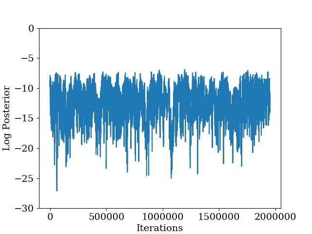
Figure 4: Trace plot of the logarithm of the posterior distribution with a burn-in of 50,000 iterations. It is apparent that the MCMC sampling is at equilibrium.

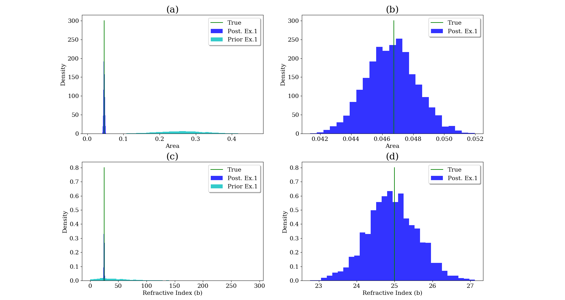
Figure 5: Parts (a) and (c) show the prior distribution in cyan, the posterior distribution in blue, and the true value in green of both, the area of the scatterer and the refractive index for Example 1. Parts (b) and (d) show a close up along the horizontal axis near the true values.

In order to show that the results obtained in Example 5 are independent of the directions of the incident field, in the next example we repeat the numerical experiment except that none of the incident directions coincide with an axis of symmetry of the obstacle.

We consider the same setting of Example 1, except that the directions in the incident field are rotated letting $\zeta=\frac{\pi}{6}$. Figure 6 compares histograms of both, the refractive index $\mathbf{b}$ and the area of the obstacle obtained in Examples 5 and 5.

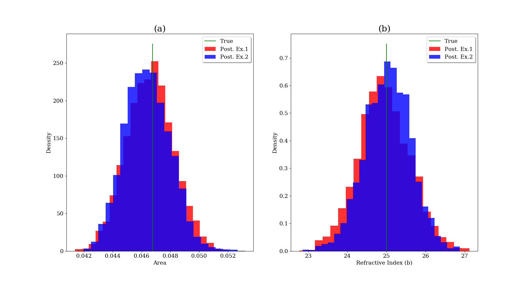
Figure 6: For examples 5 and 5; posterior distributions of the scatterer area and (b) the refractive index.

Finally, Example 5 illustrates the effect of using a finer mesh in the numerical solution of the direct problem. As expected, the variance of both, the refractive index $\mathbf{b}$ and the quantity of interest decreases if the mesh is reduced.

In this example, the configuration is taken as in Example 5, and we refined the mesh taking $N=80$, $h=0.01$. We computed 1,000,000 samples of the posterior distribution. Histograms of the posterior of both, the refractive index $\mathbf{b}$ and the area of the obstacle are shown in Figure 7 together with the respective results of Example 5. As before, the true values are shown for comparison. Figure 8 summarizes the retrieval of the scatterer in all examples above. Numerical evidence suggest that the posterior distribution is insensitive with respect to a rotation of the direction of the incident fields. On the other hand, there is a trade off between precision and computational cost as expected. Table 1 compares the true value, maximum a posteriori and conditional mean of our quantity of interest. All estimators are correct with roughly two digits. Of note, the area of the true scatterer was computed with the same resolution of the point cloud interpolation.

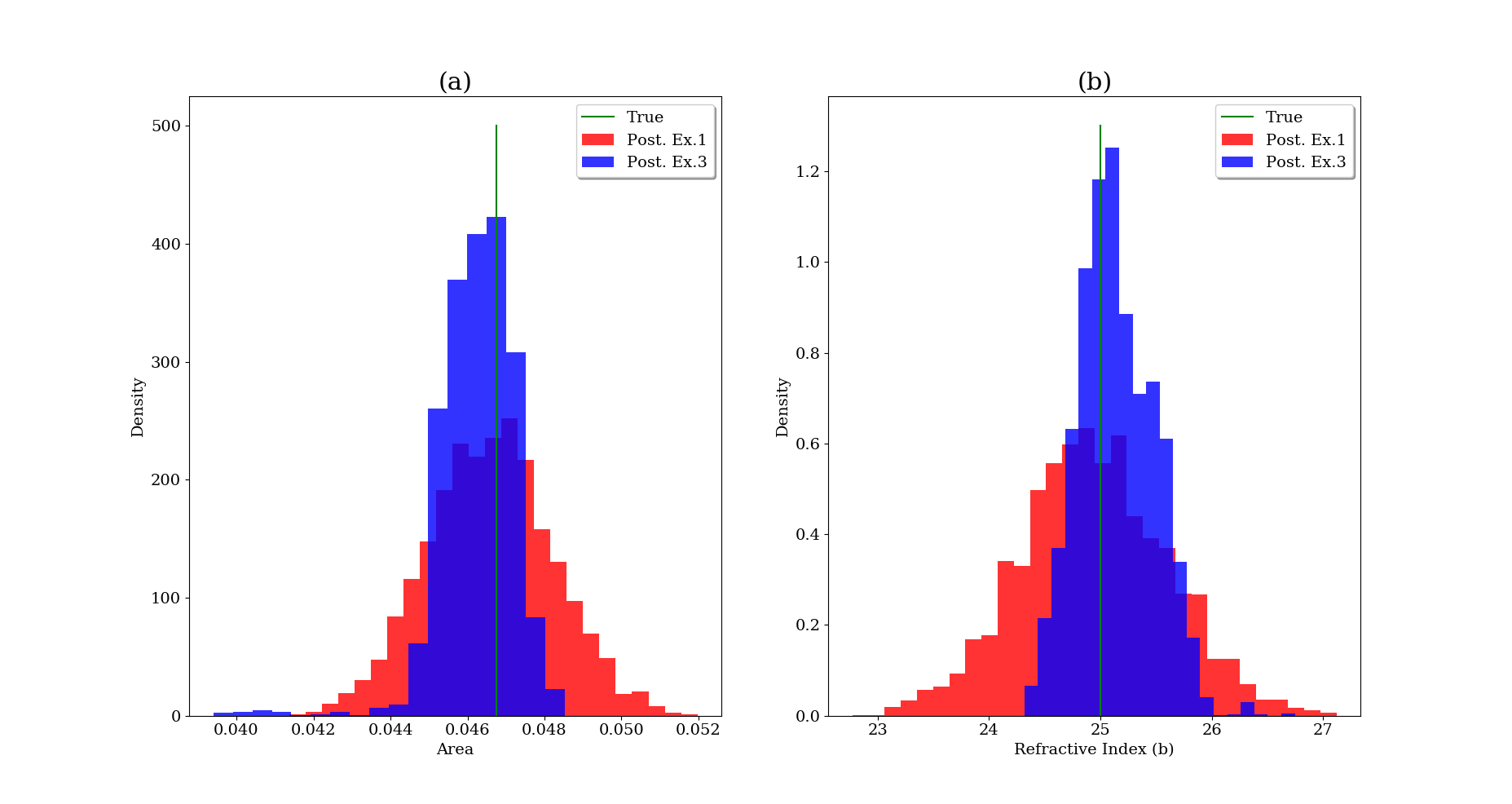
Figure 7: Example 5; posterior distributions of the scatterer area and (b) the refractive index.

We may discuss the results of this manuscript as follows: we have introduced a method, based on standard ideas of computational geometry, capable of simultaneously recovering both, the support and constant refractive index of a star-shaped scatterer. In Figures 4 through 8 and Table 1, we offer numerical evidence of the robustness of our method using a star-shaped scatterer commonly used as benchmark in the literature of inverse scattering problems under a particular data design.

On the other hand, although our method does accomplish the task of reliably solving the inverse problem, it is computationally expensive. We remark that our method is derivative free. We believe that further research on affine invariant proposals is justified i.e., a natural extension is to explore the performance of derivative informed proposals of the probability transition kernel that fulfill the affine invariant property. In general, we believe that it might be possible to further extend the idea of axiomatically imposing geometric properties on move proposals for the probability transition kernel, such as moves that commute with affine transformations of space, and then introducing examples of moves that fulfill those conditions.

Area of the scatterer
True value	Conditional Mean	Maximum a posteriori
$4.68\times 10^{-2}$	$4.66\times 10^{-2}$	$4.60\times 10^{-2}$	Example 1
	$4.64\times 10^{-2}$	$4.53\times 10^{-2}$	Example 2
	$4.63\times 10^{-2}$	$4.51\times 10^{-2}$	Example 3

Table 1: All estimators are correct with roughly two digits. Of note, the area of the true scatterer was computed with the same resolution of the point cloud interpolation.

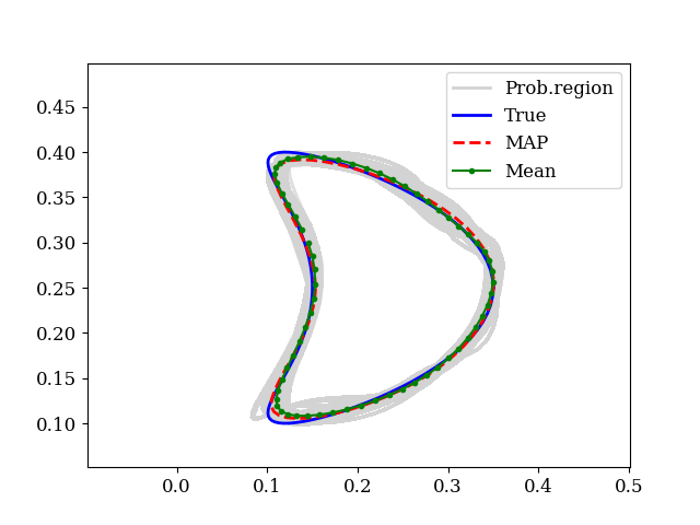
(a) Example 5

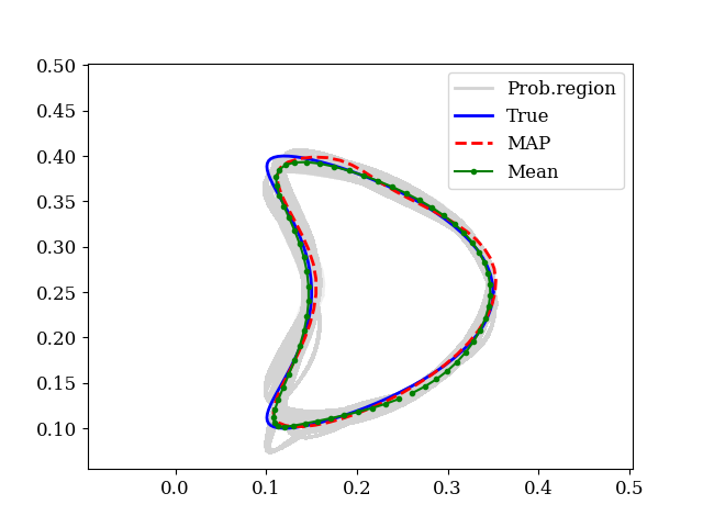
(b) Example 5

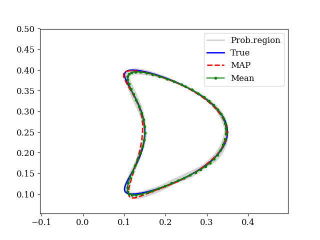
(c) Example 5

Figure 8: Numerical evidence in Examples 5 and 5 suggests that the posterior distribution is insensitive with respect to a rotation of the direction of the incident fields. On the other hand, Example 5 indicates there is a trade off between precision and computational cost as expected.

6 Conclusions

In this paper we have demonstrated a reliable method to approximate the solution of the inverse scattering problem in the case of penetrable obstacles. Of note, we can recover simultaneously the support and constant refractive index of the scatterer. Our results are based on standard ideas of computational geometry, which is a very active area of computer science with numerous applications. We consider that our findings are amenable to numerous extensions.

We believe that future work should be directed towards improving the efficiency of the method in terms of computational cost. Three possible research avenues, not necessarily in order of importance, are as follows. First, explore the performance of derivative informed proposals of the probability transition kernel that fulfill the affine invariant property. Second, defining a delayed acceptance method on the frecuency (lower wavenumber and higher wavenumber) spaces with two stages; the lower-model with a coarse mesh and the higher-model with a fine mesh. Finally, another approach might be, changing the number of points in the cloud in each level (delayed acceptance), for instance adding points in the cloud, taking more points for the interpolation of the point cloud.

References

- [1] A. M. Stuart. Inverse problems: A bayesian perspective. Acta Numerica, 19:451–559, 2010.
- [2] J Andrés Christen. Posterior distribution existence and error control in banach spaces. arXiv preprint arXiv:1712.03299, 2017.
- [3] Tan Bui-Thanh, Omar Ghattas, James Martin, and Georg Stadler. A computational framework for infinite-dimensional bayesian inverse problems part i: The linearized case, with application to global seismic inversion. SIAM Journal on Scientific Computing, 35(6):A2494–A2523, 2013.
- [4] Mark Girolami and Ben Calderhead. Riemann manifold langevin and hamiltonian monte carlo methods. Journal of the Royal Statistical Society: Series B, 73(2):123–214, 2011.
- [5] Herbert Edelsbrunner, David Kirkpatrick, and Raimund Seidel. On the shape of a set of points in the plane. IEEE Transactions on information theory, 29(4):551–559, 1983.
- [6] M Sh Birman and Mikhail Zakharovich Solomyak. Estimates of singular numbers of integral operators. Russian Mathematical Surveys, 32(1):15, 1977.
- [7] David Colton and Rainer Kress. Inverse acoustic and electromagnetic scattering theory, volume 93. Springer Science & Business Media, 2012.
- [8] J Andrés Christen and Colin Fox. A general purpose sampling algorithm for continuous distributions (the t-walk). Bayesian Analysis, 5(2):263–281, 2010.
- [9] Juan C Aguilar and Yu Chen. High-order corrected trapezoidal quadrature rules for functions with a logarithmic singularity in 2-d. Computers & Mathematics with Applications, 44(8):1031–1039, 2002.
- [10] Gennadi Vainikko. Fast solvers of the lippmann-schwinger equation. In Direct and inverse problems of mathematical physics, pages 423–440. Springer, 2000.
- [11] Lars Linsen. Point cloud representation. Univ., Fak. für Informatik, Bibliothek, 2001.
- [12] Mark Pauly, Richard Keiser, Leif P Kobbelt, and Markus Gross. Shape modeling with point-sampled geometry. In ACM Transactions on Graphics (TOG), pages 641–650. ACM, 2003.
- [13] Mark Pauly, Niloy J Mitra, and Leonidas J Guibas. Uncertainty and variability in point cloud surface data. SPBG, 4:77–84, 2004.
- [14] Mark Pauly, Leif P Kobbelt, and Markus Gross. Point-based multiscale surface representation. ACM Transactions on Graphics (TOG), 25(2):177–193, 2006.
- [15] Matthew Berger, Andrea Tagliasacchi, Lee M Seversky, Pierre Alliez, Gael Guennebaud, Joshua A Levine, Andrei Sharf, and Claudio T Silva. A survey of surface reconstruction from point clouds. In Computer Graphics Forum, pages 301–329. Wiley Online Library, 2017.
- [16] Abel Palafox, Marcos A Capistrán, and J Andrés Christen. Effective parameter dimension via bayesian model selection in the inverse acoustic scattering problem. Mathematical Problems in Engineering, 2014, 2014.
- [17] Jari Kaipio and Erkki Somersalo. Statistical and computational inverse problems, volume 160. Springer Science & Business Media, 2006.
- [18] James F Greenleaf, Mostafa Fatemi, and Michael Insana. Selected methods for imaging elastic properties of biological tissues. Annual review of biomedical engineering, 5(1):57–78, 2003.
- [19] Maria L Daza, Marcos A Capistrán, J Andrés Christen, and Lilí Guadarrama. Solution of the inverse scattering problem from inhomogeneous media using affine invariant sampling. Mathematical Methods in the Applied Sciences, 2016.
- [20] Abel Palafox, Marcos Capistrán, and J Andrés Christen. Point cloud-based scatterer approximation and affine invariant sampling in the inverse scattering problem. Mathematical Methods in the Applied Sciences, 40(9):3393–3403, 2017.
- [21] Andreas Kirsch and R Kress. Two methods for solving the inverse acoustic scattering problem. Inverse problems, 4(3):749, 1988.