Abstract

The inverse problem methodology is a commonly-used framework in the sciences for parameter estimation and inference. It is typically performed by fitting a mathematical model to noisy experimental data. There are two significant sources of error in the process: 1.  Noise from the measurement and collection of experimental data and 2.  numerical error in approximating the true solution to the mathematical model. Little attention has been paid to how this second source of error alters the results of an inverse problem. As a first step towards a better understanding of this problem, we present a modeling and simulation study using a simple advection-driven PDE model. We present both analytical and computational results concerning how the different sources of error impact the least squares cost function as well as parameter estimation and uncertainty quantification. We investigate residual patterns to derive an autocorrelative statistical model that can improve parameter estimation and confidence interval computation for first order methods. Building on the results of our investigation, we provide guidelines for practitioners to determine when numerical or experimental error is the main source of error in their inference, along with suggestions of how to efficiently improve their results.

[Numerical Error in Inverse Problems for PDEs]The Influence of Numerical Error on an Inverse Problem Methodology in PDE Models

John T. Nardini^1,2, D. M. Bortz¹

1 Introduction

Differential Equations are frequently used to study scientific systems. When there are multiple independent variables influencing this system (such as time and space), then a partial differential equation (PDE) is the appropriate modeling framework. Due to their complicated nature, deriving an analytical solution to a PDE model is frequently difficult or impossible, so scientists must use numerical methods to approximate the true solution. How the error from this approximation influences some aspects of an inverse problem, such as parameter estimation and uncertainty quantification, is an important and poorly-understood problem. We will focus on a deterministic inverse problem in this study, but approximation errors in determining the likelihood are of significant concern in Bayesian methods as well  [6]. There have been some notable previous efforts to elucidate these questions. For example, Banks and Fitzpatrick  [2] proved the asymptotic consistency of the parameter estimator for least squares estimation in the presence of numerical approximation error, and Xue et al.  [15] derived the asymptotic distribution of this estimator when a numerical approximation is used to for an ordinary differential equation model.

In a previous study on parameter estimation, Ackleh and Thibodeaux  [1] consider an advection-driven model of erythyropoiesis (an important step in red blood cell development) with three independent variables of time, maturity, and space. The authors show that using an upwind scheme for computation during an inverse problem is asymptotically well-posed for parameter estimation as the numerical step size used, $h$, approaches zero. In practice, however, one cannot let $h$ approach zero but must choose a finite value of $h$ to estimate the parameters with. Furthermore, advection equations such as that used in  [1] are known to cause a multitude of numerical issues, especially when the true solution is discontinuous  [7, 10, 13]. The upwind method is a popular choice to simulate these problems because it can avoid spurious oscillations by satisfying the Courant-Friedrichs-Lewy (CFL) condition, but this method also causes its own difficulties by admitting numerical diffusion near points of discontinuity  [8, 10].

The work in these publications raise a multitude of questions to consider when performing an inverse problem. How do the least squares cost function and parameter estimator behave as numerical error decreases? For the step size used, what is the dominant source of error in the cost function computation? If numerical error dominates, can we use residuals as a way to update how we compute the cost function and improve the inverse problem’s results? How do we know if the chosen numerical method can accurately estimate parameters? How do the results change based on properties of the model’s solution?

In this study, we will use a simple advection equation to demonstrate the impact of numerical error from several finite difference and finite volume methods on an inverse problem methodology. To compare the influence of numerical versus experimental error in this study, we will fit these computations to data sets that have been artificially generated from the analytical solution with varying levels of experimental noise. We begin in Section  2 by introducing some preliminary information, including the equation under consideration and its analytical solution, how we generate the artificial data sets, and the numerical methods used in this study. In Section  3, we introduce the inverse problem methodology and discuss the asymptotic results for the parameter estimator and numerical cost function used in this framework. In Section  4, we discuss our results in using these numerical methods to estimate parameters from the data sets. We use residual analysis in Section  5 to demonstrate how numerical error from first order numerical methods leads to an autocorrelated error structure when comparing the model to data. To address this issue, we derive an autocorrelative statistical model to describe how this numerical error propagates throughout the inverse problem. We further demonstrate how this autocorrelated statistical model can be used to improve confidence interval computation and parameter estimation. Based on these results, we provide some suggestions and guidance for practitioners in Section  6 to ensure that the results of their inverse problem routines are as accurate as possible. We make concluding remarks and discuss future work in Section  7.

2 Mathematical Preliminaries

In this section, we detail some necessary information regarding our inverse problem methodology. We discuss the advection equation and choice of parameterization in Section  2.1. In Section  2.2, we will present some notation used throughout this work. We present how we generate artificial data for this study in Section  2.3. In Section  2.4, we discuss the numerical schemes that we will use in this study.

2.1 PDE Model Equation

We will consider an advection equation in one spatial dimension. We define our spatial domain as $X=[0,1]$, the temporal domain as $T=[0,10],$ and the parameter value domain as $\Theta=\mathbb{R}^{k_{\theta}}$ for $k_{\theta}$ denoting the number of parameters to be estimated. The advection equation is given by

$$u_{t}+(g(x;\theta)u)_{x} =0,\ u=u(t,x;\theta)$$ (1)

$$u(t=0,x;\theta) =\phi(x)$$

$$x\in X,t\in T ,\theta\in\Theta$$

where subscripts denote differentiation, $g(x;\theta)$ is a spatially-dependent advection rate that is parameterized by the vector $\theta$, $\phi(x)$ is the initial condition, and $u(t,x;\theta)$ denotes the quantity of interest at time $t$ and spatial location $x$ that is also parameterized by $\theta$. We will suppress the dependence of $g(x)$ and $u(t,x)$ on $\theta$ throughout this study when this dependence can be implicitly understood.

The method of characteristics can be used to show the analytical solution to Equation (1) of

$$u_{0}(t,x)=\begin{cases}\dfrac{g(\sigma^{-1}(-t,x))}{g(x)}\phi(\sigma^{-1}(-t,x))&\sigma^{-1}(t,0)\leq x\leq 1\\ 0&\text{otherwise}\end{cases}$$ (2)

where $\sigma^{-1}(t,x)$ is the characteristic curve that satisfies the initial value problem

$$\dfrac{\partial}{\partial t}\sigma^{-1}(t,x)=g\left(\sigma^{-1}(t,x)\right),\ \sigma^{-1}(t=0,x)=x.$$

See  [14] for more information about deriving this analytical solution and  [9] for an illustrative example of this concept involving biochemical activation during wound healing. We choose the rate of advection

$$g(x)=\alpha\sqrt[\beta]{x},\ \ \ \alpha,\beta>0$$

for $\theta=(\alpha,\beta)^{T}\in\Theta=\mathbb{R}^{2}$. The choice of $g(x)$ above yields the characteristic curves

$$\sigma^{-1}(t,x)=\left[\alpha(1-\nicefrac{{1}}{{\beta}})t+x^{1-\nicefrac{{1}}{{\beta}}}\right]^{\nicefrac{{\beta}}{{(\beta-1)}}}.$$

We will consider two initial conditions in this study to demonstrate how spatial continuity influences numerical convergence and the inverse problem results. To demonstrate the behavior for a discontinuous solution, we will focus on simulations with a discontinuous initial condition given by the step function

$$\phi_{d}(x)=\begin{cases}5&x\leq 0.2\\ 0&\text{otherwise}\end{cases}$$

To illustrate how the results change for a continuous solution, we will also consider the Gaussian-shaped initial condition given by

$$\phi_{c}(x)=e^{-\left(\nicefrac{{x-0.2}}{{\sqrt{.005}}}\right)^{2}}.$$

We will focus on the results for $\phi(x)=\phi_{d}(x)$ in the main body of this document, with the corresponding results for $\phi(x)=\phi_{c}(x)$ in the supporting material. We will make note of how the results change between these two initial conditions when appropriate.

2.2 Explanation of Notation

Note that throughout this work, $M$ and $N$ denote the number of time and spatial points provided in an artificial data set, respectively. We will denote the numerical step size as $h$, which will determine the number of grid points used during numerical computations. It is important to realize that $h$, $M$, and $N$ are all independent of one another.

Our data sets will be provided on the uniform partitions of $T\times X$ given by $T^{M}\times X^{N}$, where

$$T^{M}=\{t_{i}\}_{i=1}^{M}=10\left\{\nicefrac{{(i-1)}}{{M}}\right\}_{i=1}^{M},\ \ X^{N}=\{x_{j}\}_{j=1}^{N}=\left\{\nicefrac{{j-1}}{{N}}\right\}_{j=1}^{N}.$$

We will write a given data set as the $M\times N$ matrix, $Y$. The $(i,j)th$ entry of $Y$ is given by

$$\left[Y\right]_{i,j}=y_{i,j},$$

where $y_{i,j}$ denotes the observation of the data at time $t_{i}$ and location $x_{j}.$ We will denote the analytical solution to Equation (1) with parameter value $\theta$ on $T^{M}\times X^{N}$ as the $M\times N$ matrix, $U_{0}(\theta)$, with $(i,j)th$ entry

$$\left[U_{0}(\theta)\right]_{i,j}=u_{0}(t_{i},x_{j};\theta).$$

We will denote a numerical computation that has been computed with numerical step size $h$ and parameter value $\theta$ and then interpolated to $T^{M}\times X^{N}$ as the $M\times N$ matrix $U(h,\theta)$ with $(i,j)th$ entry

$$\left[U(h,\theta)\right]_{i,j}=u(t_{i},x_{j};h,\theta).$$

Arrows on top of these sets will denote their vectorizations, e.g., the vector $\vec{U}_{0}(\theta)$ will denote the $MN\times 1$ vectorization of $U_{0}(\theta)$. We write $u_{0}(t,x)$ and $u(t,x;h)$ to denote these functions on the domain $T\times X.$

The matrix $\nabla_{\theta}U_{0}(\theta)$ is the $MN\times k_{\theta}$ matrix vectorization of the gradient of the analytical solution with respect to $\theta$ (also known as the sensitivities). The matrix $\nabla_{\theta}U(h,\theta)$ will denote the numerically-computed $MN\times k_{\theta}$ matrix for these sensitivity equations. The vector $\vec{\epsilon}$ denotes the $MN\times 1$ vector of realizations of the Gaussian error terms.

We will perform our inverse problem for values of $h$ given by $h_{i}=\left(10\times 2^{i-1}\right)^{-1},\ i=1,\ldots,7$. For each value of $h$, we also use temporal step size $k=\lambda h$ for a value of $\lambda$ that will satisfy the CFL condition, which is a necessary (but not sufficient) condition for numerical stability. When describing a vector of step sizes, we will let $\boldsymbol{h}=(h_{1},...,h_{7})^{T}$. In a slight abuse of notation, we will write a vector of function values, $f(h)$, at different step sizes as $f(\boldsymbol{h})=(f(h_{1}),...,f(h_{7}))^{T}.$

2.3 Artificial Data Generation

We generate several artificial data sets from $U_{0}(\theta_{0})$ for this study. These data sets are created by adding Gaussian noise to the analytical solution, written as the statistical model

$$y_{i,j}=u_{0}(t_{i},x_{j};\theta_{0})+\epsilon_{i,j},\ \epsilon_{i,j}\stackrel{{\scriptstyle i.i.d.}}{{\sim}}\mathcal{N}(0,\eta^{2}),\ \ i=1,..,M,\ j=1,..,N$$ (3)

for some “true” parameter value, $\theta_{0}\in\Theta.$ We will generate data sets with different values of $N$ and $\eta$ for both initial conditions, $\phi_{d}(x)$ and $\phi_{c}(x)$. Note that $M$ will be fixed at 6 for simplicity in all data sets considered: we performed a similar analysis for data sets generated with larger values of $M$ but found that the final results to be similar to the results for increasing $N$ (results not shown). We choose $\theta_{0}=(0.3,0.5)^{T}$ for data sets where $\phi(x)=\phi_{d}(x)$ and $\theta_{0}=(0.3,0.4)^{T}$ for data sets where $\phi(x)=\phi_{c}(x)$. An example data set is depicted against $u_{0}(t,x;\theta_{0})$ for $\eta^{2}=0.01,N=11$ in Figure  1.

We will also perform the inverse problem for multiple data sets with varying numbers of data points and data error levels. For $\phi(x)=\phi_{d}(x),$ we consider data sets for $N=\{11,30,51\}$ and $\eta=\{0,10^{-1},1.5\times 10^{-1},2\times 10^{-1},3\times 10^{-1},5\times 10^{-1},1\}.$ For $\phi(x)=\phi_{c}(x),$ we consider data sets for $N=\{11,31,51\}$ and $\eta=\{0,10^{-4},5\times 10^{-4},10^{-3},10^{-2},5\times 10^{-2},10^{-1},2\times 10^{-1}\}.$ We will only show some results in the main text for ease of interpretation, but all results for all data sets are provided in the supporting material.

Figure 1: Artificial data from Equations (2) and (3) for $\eta=0.1,N=11,M=6$, and $\phi(x)=\phi_{d}(x).$ The solid lines denote the analytical solution given by Equation (2) and the various markers denote the artificial data points. Red asterisks denote $t=0,$ green squares denote $t=2,$ blue x’s denote $t=4,$ cyan triangles denote $t=6,$ black triangles denote $t=8,$ and magenta dots denote $t=10.$

2.4 Numerical Methods and Order of Convergence

We will consider four commonly-used numerical schemes to approximate the solution to Equation (1). These four schemes are the upwind, Lax-Wendroff, and Beam-Warming methods, as well as the upwind method with flux limiters. The first three methods are discussed and presented in the popular monograph by Leveque  [8], and the final method is discussed in  [10, $\S 16.2$] and  [13].

A common practice in numerical analysis is to compute the order of convergence for a numerical scheme. Guided by  [8], we define the error for a numerical scheme as

$$E(h;\theta)=\|\vec{U}(h,\theta)-\vec{U}_{0}(\theta)\|_{1},$$

where $\|\cdot\|_{1}$ denotes the 1-norm in $\text{$\mathbb{R}$}^{MN}$. The upwind method is first order accurate when $u_{0}(t,x)$ is differentiable, meaning that $E(h)\approx\mathcal{O}(h^{1})$ for $h$ sufficiently small. The Lax-Wendroff and beam warming method are second order accurate so that $E(h)\approx\mathcal{O}(h^{2})$ under similar assumptions.

While these schemes are often referred to as first- or second-order accurate, this is only true when the analytical solution, $u_{0}(t,x)$, is continuous with respect to $x$. When $u_{0}(t,x)$ is discontinous, the order for these schemes can be computed using the theory of modified equations (described in  [10, $\S$ 11]). This theory can show that the upwind method is of order 1/2, and the Lax-Wendroff and Beam-Warming methods are of order 2/3 when $u_{0}(t,x)$ is discontinuous. This theory can also be used to demonstrate that the upwind method will add numerical diffusion error when used to approximate the solution to Equation (1). Similarly, the Lax-Wendroff and Beam-Warming methods will add numerical dispersion error when used to approximate the solution to Equation (1). In both cases, the rates of diffusion or dispersion disappear as $h\rightarrow 0$. These numerical error patterns can be clearly seen in Figure  4.1.

This information from the theory of modified equations has prompted our use of the following definition for the order of convergence throughout our study.

Definition 1.

A numerical method has order of convergence $p$ if, for $h$ small,

$$u(t,x;h,\theta)\approx u_{0}(t,x;\theta)+h^{p}w(t,x;h)$$

for some positive value, $p$, on all compact subsets of $\Theta_{comp}\subset\Theta$, where $\|w(t,x;h)\|_{\infty}$ is uniformly bounded for small values of $h$. Furthermore, for every $h$, $u(x,t;h,\theta):\Theta\rightarrow L^{1}(T\times X\rightarrow\mathbb{R})$ is continuous with respect to $\theta$.

Note that this definition is stronger than the standard definition of numerical order of convergence, and it immediately implies $E(h,\theta)=\mathcal{O}(h^{p})$ so long as $T\times X$ is compact. For the first (second) order methods, $w(t,x)$ represents numerical diffusion (dispersion) from the approximation scheme.

From the observation that $|u(t,x;h,\theta)-u_{0}(t,x;\theta)|\leq Ch^{p}$ for all $t,x$ from the above definition, where ${\displaystyle C=\sup_{(t,x)\in T\times X}|w(t,x;h)|}$, we will rewrite the above equation as

$$u(t,x;h,\theta)=u_{0}(t,x;\theta)+\mathcal{O}(h^{p})$$ (4)

for ease of notation. To estimate the order of convergence for a numerical scheme throughout this study, we will find the best-fit line for the natural log of the error, $\ln(E(\boldsymbol{h}))$, against $\ln(\boldsymbol{h})$. The slope of this line will estimate $p$, which we will denote as the numerical order of convergence.

Flux limiters are a popular tool to aid numerical schemes for advection equations with discontinuous solutions  [12, 13]. When flux limiters are used, the spatial gradient at each computational point is estimated at each time point. These estimations are used to make the numerical scheme approximately second-order accurate near smooth spatial points and first order accurate near points of discontinuity. An upwind scheme with flux limiters thus prevents dispersive oscillations from propagating near the discontinuity, and instead allows a small amount of numerical diffusion in this region. In this study, we will use the Van-Leer flux limiter  [10].

In Table  2, we depict the calculated values of $p$ for $\phi(x)=\phi_{d}(x)$ and $\theta=\theta_{0}$ and see that our calculated numerical order of convergence for the upwind scheme is consistent with the theory (close to 1/2), but the order for the Lax-Wendfroff and Beam-Warming schemes are smaller and larger than expected, respectively ($p$ is calculated as 0.4737 for Lax-Wendfroff and 0.7876 for Beam-Warming, when the theory suggests these both should be 2/3). The upwind scheme with flux limiters has a calculated numerical order of convergence of 0.9570. To the best of our knowledge, there are no analytical results for the order of the upwind scheme with flux limiters when calculating a discontinuous solution. We show in Table S1 in the supporting material that the calculated numerical orders of convergence for $\phi(x)=\phi_{c}(x)$ are consistent with theory for continuous solutions. Here, we calculate the order of convergence for the upwind with flux limiters scheme to be 0.9183.

3 Asymptotic Properties of the Inverse Problem

For a given data set, $Y,$ and (analytical) mathematical model, $U_{0}(\theta)$, the ordinary least squares (OLS) cost function given by

$$J^{M,N}(\theta)=\dfrac{1}{MN}\sum_{i=1}^{M}\sum_{j=1}^{N}(y_{i,j}-u_{0}(t_{i},x_{j};\theta))^{2},$$ (5)

is a means to estimate the disparity between the data and model. In the inverse problem framework, one may compute an estimate, $\hat{\theta}_{OLS}^{M,N}$, of the true parameter vector, $\theta_{0}$, by finding

$$\hat{\theta}_{OLS}^{M,N}=\arg\min_{\theta\in\Theta_{ad}}J^{M,N}(\theta).$$

In practice, we do not know $U_{0}(\theta)$ and must approximate it with the numerical computation, $U(h,\theta)$. In this case, the numerical OLS cost function,

$$J^{M,N}(h,\theta)=\dfrac{1}{MN}\sum_{i=1}^{M}\sum_{j=1}^{N}(y_{i,j}-u(t_{i},x_{j};h,\theta))^{2},$$ (6)

is a means to estimate the disparity between the data and numerical computation. In this work, we will compute estimates, $\hat{\theta}_{OLS}^{M,N}(h)$, of the true parameter vector, $\theta_{0}$, by finding

$$\hat{\theta}_{OLS}^{M,N}(h)=\arg\min_{\theta\in\Theta_{ad}}J^{M,N}(h,\theta),$$

where $\Theta_{ad}\subset\Theta$ denotes the space of admissible parameter values. For the optimization in this study, we used an interior point algorithm as implemented in MATLAB’s fmincon function to find $\hat{\theta}_{OLS}^{M,N}(h)$.

In the rest of this section, we will discuss asymptotic properties of the inverse problem as the number of data points increases ($M,N\rightarrow\infty$) and the step size decreases ($h\rightarrow 0$). In Section  3.1, we discuss the asymptotic distribution of the estimator, $\hat{\theta}_{OLS}^{M,N}(h)$, and in Section  3.2, we discuss the convergence of the numerical cost function, $J^{M,N}(h,\hat{\theta}_{OLS}^{M,N}(h)).$

3.1 Theory of $\hat{\theta}_{OLS}^{M,N}(h)$

The asymptotic properties of $\theta_{OLS}^{M,N}$ have been widely discussed and are provided in Theorem 2.1 from  [11] (which is stated in  A for convenience). In  [2], it is further shown that $\hat{\theta}_{OLS}^{M,N}(h)$ is a consistent estimator, meaning that $\hat{\theta}_{OLS}^{M,N}(h)\rightarrow\theta_{0}$ almost surely as $M,N\rightarrow\infty$ and $h\rightarrow 0$. This proof requires $\Theta_{ad}$ to be a compact subset of $\Theta$; accordingly, we have chosen $\Theta_{ad}=[0,10]\times[0,10]$. This proof also requires the following reasonable assumptions.

1. The finite measures $\chi$ and $\nu$ exist on $X$ and $T$ such that

   $$\dfrac{1}{MN}\sum_{i=1}^{M}\sum_{j=1}^{N}v(t_{i},x_{j})\rightarrow\int_{X}\int_{T}v(t,x;\theta)d\nu(t)d\chi(x)$$

   for any $v\in L^{1}(T\times X\rightarrow\mathbb{R})$ as $M,N\rightarrow\infty$.

2. The functional

   $$J^{*}(\theta)=\int_{X}\int_{T}(u_{0}(t,x;\theta_{0})-u_{0}(t,x;\theta))^{2}d\nu(t)d\chi(x)$$

   has a unique minimizer in $\Theta_{ad}$ at $\theta_{0}.$

The theorem for $\theta_{OLS}^{M,N}$ in  [11] does not account for numerical errors in the model solution while the theory for $\hat{\theta}_{OLS}^{M,N}(h)$ in  [2] does not consider the implications of the numerical order of solution convergence.

We now state our main theoretical result on the behavior of $\theta_{OLS}^{M,N}(h)$ as numerical accuracy increases. The following corollary extends the above theory to account for the fact that the solution to the PDE model is being approximated with an order $p$ scheme.

Corollary 2.

Consider a numerical scheme for a differential equation that is order $p$ accurate for $u_{0}(t,x)$ and $\nabla_{\theta}u_{0}(t,x;\theta)$. Under the assumptions (A1) and (A2), we have the asymptotic distribution for $\theta_{OLS}^{M,N}(h)$ as $M,N\rightarrow\infty$ and $h\rightarrow 0$ given by

$$\hat{\theta}_{OLS}^{M,N}(h)\sim\mathcal{N}(\theta_{0},\eta^{2}V_{h}).$$

The entries of $V_{h}$ are $\mathcal{O}(h^{p})$ convergent to the entries of $V=(\nabla_{\theta}U_{0}(\theta_{0})^{T}\nabla_{\theta}U_{0}(\theta_{0}))^{-1}$, which is the covariance matrix in the absence of numerical error.

Proof.

When $\theta$ is near $\theta_{0},$ we Taylor expand to see

$$\vec{U}(h,\theta) \approx\vec{U}(h,\theta_{0})+\nabla_{\theta}U(h,\theta_{0})[\theta-\theta_{0}],$$

and then use our assumptions on the numerical orders of convergence to find

$$\vec{U}(h,\theta)\approx\vec{U}_{0}(\theta_{0})+\mathcal{O}(h^{p})+[\nabla_{\theta}U_{0}(\theta_{0})+\mathcal{O}(h^{p})][\theta-\theta_{0}].$$

The numerical cost function then takes the form

$$J_{OLS}(h,\theta) =\|\vec{Y}-\vec{U}(h,\theta)\|^{2}$$

$$\approx\left\|\vec{Y}-\vec{U}_{0}(\theta_{0})-\mathcal{O}(h^{p})-[\nabla_{\theta}U_{0}(\theta_{0})+\mathcal{O}(h^{p})][\theta-\theta_{0}]\right\|^{2}.$$

The first $\mathcal{O}(h^{p})$ term is independent of $\theta$ on $\Theta_{ad}$, so minimizing $J_{OLS}(h,\theta)$ is equivalent to minimizing

$$\|\vec{Z}-X_{h}\beta\|^{2},$$

where $\vec{Z}=\vec{Y}-\vec{U}_{0}(\theta_{0})$, $X_{h}=\nabla_{\theta}U_{0}(t,x;\theta_{0})+\mathcal{O}(h^{p})$, and $\beta=\theta-\theta_{0}$. The above has the minimizer

$$\hat{\beta}=\left(X_{h}^{T}X_{h}\right)^{-1}X_{h}^{T}\vec{Z},$$ (7)

which is normally distributed because it is a linear combination of normal random variables. Assumptions $(A1)$ and $(A2)$ ensure that $\hat{\theta}_{OLS}^{M,N}(h)$ is consistent for estimating $\theta_{0}$ as $h\rightarrow 0$ and $M,N\rightarrow\infty$  [2]. Once $\hat{\theta}_{OLS}^{M,N}(h)$ is close to $\theta_{0},$ we have that

$$\hat{\theta}_{OLS}^{M,N}(h)\approx\mathcal{N}(\theta_{0},\eta^{2}(X_{h}^{T}X_{h})^{-1}),$$

where the mean and covariance can be calculated directly from their definitions.

Determining the convergence (in any matrix norm) of $V_{h}=(X_{h}^{T}X_{h})^{-1}$ to the inverse of $\nabla_{\theta}U_{0}(\theta_{0})^{T}\nabla_{\theta}U_{0}(\theta_{0})$ is a difficult problem. However, by using a result from the analysis of numerical algorithms  [5], we can draw some conclusions about the individual entries of $V_{h}$. Consider the $(i,j)th$ entry of $X_{h}^{T}X_{h}:$

$$|[X_{h}^{T}X_{h}]_{i,j}| =|(\nabla_{\theta}U_{0}(t_{i},x_{j};\theta_{0})+\mathcal{O}(h^{p}))^{T})(\nabla_{\theta}U_{0}(t_{i},x_{j};\theta_{0})+\mathcal{O}(h^{p}))|$$

$$=|\nabla_{\theta}U_{0}(t_{i},x_{j};\theta_{0})^{T}\nabla_{\theta}U_{0}(t_{i},x_{j};\theta_{0})+\mathcal{O}(h^{p})\nabla_{\theta}U_{0}(t_{i},x_{j};\theta_{0}))+\mathcal{O}(h^{2p})|,$$

meaning that this entry converges to its corresponding entry of $\nabla_{\theta}U_{0}(\theta_{0})^{T}\nabla_{\theta}U_{0}(\theta_{0})$ with an order of convergence $p.$ Then, using results from  [5, $\S$ 13.1], we can show

$$\left|\left[(\nabla_{\theta}U_{0}(\theta_{0})^{T}\nabla_{\theta}U_{0}(\theta_{0}))^{-1}-(X_{h}^{T}X_{h})^{-1}\right]{}_{i,j}\right|\leq$$

$$\mathcal{O}(h^{p})\left|\left[(\nabla_{\theta}U_{0}(\theta_{0})^{T}\nabla_{\theta}U_{0}(\theta_{0}))^{-1}\right]_{i,j}\right|\left|\left[\nabla_{\theta}U_{0}(\theta_{0})^{T}\nabla_{\theta}U_{0}(\theta_{0})\right]_{i,j}\right|\left|\left[(\nabla_{\theta}U_{0}(\theta_{0})^{T}\nabla_{\theta}U_{0}(\theta_{0}))^{-1}\right]_{i,j}\right|$$

$$+\mathcal{O}(h^{2p}).$$

Thus, each entry of $V_{h}$ will will converge to its corresponding entry of $V$ as $\mathcal{O}(h^{p})$. ∎

3.2 Convergence of $J^{M,N}(h,\theta)$

The least squares cost function from Equation (6) is widely used for inverse problems  [4]. In this section, we discuss the asymptotic properties of this function as $h\rightarrow 0$ and $M,N\rightarrow\infty$ to elucidate our results in future sections.

Observe that by combining Equations (3) and (6), the cost function can be rewritten as

$$J^{M,N}(h,\theta) =\dfrac{1}{MN}\sum_{i,j=1}^{M,N}[u_{0}(t_{i},x_{j};\theta_{0})+\epsilon_{i,j}-u(t_{i},x_{j};h,\theta)+u_{0}(t_{i},x_{j};\theta)-u_{0}(t_{i},x_{j};\theta)]^{2}$$ (8)

$$=A+B+C+D+E+F,$$

where

$$A =\dfrac{1}{MN}\sum_{i,j=1}^{M,N}\mathcal{\epsilon}_{i,j}^{2}$$

$$B =\dfrac{1}{MN}\sum_{i,j=1}^{M,N}[u_{0}(t_{i},x_{j};\theta_{0})-u_{0}(t_{i},x_{j};\theta)]^{2}$$

$$C =\dfrac{1}{MN}\sum_{i,j=1}^{M,N}[u_{0}(t_{i},x_{j};\theta)-u(t_{i},x_{j};h,\theta)]^{2}$$

$$D =\dfrac{2}{MN}\sum_{i,j=1}^{M,N}\mathcal{\epsilon}_{i,j}(u_{0}(t_{i},x_{j};\theta_{0})-u_{0}(t_{i},x_{j};\theta))$$

$$E =\dfrac{2}{MN}\sum_{i,j=1}^{M,N}\mathcal{\epsilon}_{i,j}(u_{0}(t_{i},x_{j};\theta)-u(t_{i},x_{j};h,\theta))$$

$$F =\dfrac{2}{MN}\sum_{i,j=1}^{M,N}[(u_{0}(t_{i},x_{j};\theta)-u(t_{i},x_{j};h,\theta))(u_{0}(t_{i},x_{j};\theta_{0})-u_{0}(t_{i},x_{j};\theta))]$$ (9)

We thus observe that the numerical cost function can be broken down into six separate terms, each of which converges. The two following lemmas discuss the asymptotic limits and orders of convergence for terms $A$ through $F$ as data increases and as numerical accuracy increases.

Lemma 3.

If the numerical method is order $p$ accurate for $u_{0}(t,x)$ and $\nabla_{\theta}u_{0}(t,x)$, then the terms A-F from Equation (9) will behave as follows as $h\rightarrow 0$:

$$A\approx\mathcal{O}(1),\ B\approx\mathcal{O}(h^{p}),\ C\approx\mathcal{O}(h^{2p}),\ D\approx\mathcal{O}(h^{p/2}),\ E\approx\mathcal{O}(h^{p}),\ F\approx\mathcal{O}(h^{3p/2}).$$

Proof.

See  B.1. ∎

Lemma 4.

If the numerical method is order $p$ accurate for $u_{0}(t,x)$ and $\nabla_{\theta}u_{0}(t,x)$, then the terms A-F from Equation (9) will behave as follows as $M,N\rightarrow 0$:

$A$ will converge to 0 with order $\mathcal{O}(1/\sqrt{MN})$. $B$ will converge to the functional $J^{*}(\theta)$ with order $\mathcal{O}(1/(MN)).$ C is independent of $M$ and $N$. D will converge to 0 with order $\mathcal{O}(1/(\sqrt{MN}))$. E will Converge to 0 with order $\mathcal{O}(1/(\sqrt{MN}))$. $F$ will converge to an $\mathcal{O}(h^{p})$ term with order $\mathcal{O}(1/(MN))$.

Proof.

See  B.2. ∎

These two lemmas are summarized in Table  1.

	Asymptotic Properties ($h\rightarrow 0$)	Asymptotic Properties ($M,N\rightarrow\infty$)
A	$\mathcal{O}(1)$	Converges to $\eta^{2}$ with order $\mathcal{O}(1/\sqrt{MN})$
B	$\mathcal{O}(h^{p})$	Converges to $J^{*}(\theta)$ with order $\mathcal{O}(1/(MN))$
C	$\mathcal{O}(h^{2p})$	independent of $M,N$
D	$\mathcal{O}(h^{p/2})$	Converges to 0 with order $\mathcal{O}(1/(\sqrt{MN}))$
E	$\mathcal{O}(h^{p})$	Converges to 0 with order $\mathcal{O}(1/(\sqrt{MN}))$
F	$\mathcal{O}(h^{3p/2})$	Converges to an $\mathcal{O}(h^{p})$ term with order $\mathcal{O}(1/(MN))$

Table 1: Asymptotic limits for the six terms comprising the numerical cost function given by equation (6) as numerical accuracy increases ($h\rightarrow 0$) and as the number of data points increases ($M,N\rightarrow\infty$).

4 Inverse Problem Results

In this section, we present and discuss the numerical results for our inverse problems as $h\rightarrow 0$ and $N\rightarrow\infty.$ In Section  4.1, we discuss the profiles of the numerical simulations that led to these results. In Sections  4.2 and  4.3, we discuss the asymptotic behavior of $J^{M,N}(h,\hat{\theta}_{OLS}^{M,N}(h))$ and $\hat{\theta}_{OLS}^{M,N}(h)$, respectively.

4.1 Numerical Simulation Profiles

In Figure  4.1, we depict a selection of best-fit plots of $u(t,x;h,\hat{\theta}_{OLS}^{M,N}(h))$ against their corresponding artificial data sets (for all four schemes) for $\phi(x)=\phi_{d}(x).$ As expected, the first order upwind scheme is diffusive, and the second order methods are dispersive. The Lax-Wendroff method is excessively dispersive, as it displays many small oscillations but still fits the general trend of the data. The Beam-Warming method yields more accurate profile simulations than the Lax-Wendroff method, but it does have a negative portion just after the front. The upwind method with flux limiters provides the most realistic profile, as it maintains a sharp front with a nonnegative profile.

Numerical solution profiles (solid lines) plotted against artificial data (dots) for the four schemes considered when $\phi(x)=\phi_{d}(x)$ for two different step sizes. Red asterisks denote $t=0,$ green squares denote $t=2,$ blue x’s denote $t=4,$ cyan triangles denote $t=6,$ black triangles denote $t=8,$ and magenta dots denote $t=10.$ The solid curves denote $u(t,x;h,\hat{\theta}_{OLS}^{M,N}(h))$ at these time points. In the titles, “LaxWend” corresponds to the Lax-Wendroff method, “BeamWarm” corresponds to the Beam-Warming Method, and “UpwindFL” corresponds to the Upwind method with flux limiters.

4.2 Behavior of Numerical Cost Function

In Figure  2, we depict log-log plots of $J^{M,N}(\boldsymbol{h},\hat{\theta}_{OLS}^{M,N}(\boldsymbol{h}))$ against $\boldsymbol{h}$ for an initial condition of $\phi(x)=\phi_{d}(x)$. Here, we observe that the cost function converges to $\eta^{2}$ as $h\rightarrow 0$, which is consistent with the theory from Table  1. This observation suggests that numerical error dominates over experimental error until $J^{M,N}(h,\hat{\theta}_{OLS}^{MN}(h))$ reaches $\eta^{2}$, at which point experimental error becomes the dominant term in $J^{M,N}(h,\hat{\theta}_{OLS}^{MN}(h))$. We thus suggest that if $J^{M,N}(h,\hat{\theta}_{OLS}^{M,N}(h))$ decreases with $h$ , then one can further decrease the value of the cost function with continued grid refinement. We depict the log-log plots of $J^{M,N}(\boldsymbol{h},\hat{\theta}_{OLS}^{M,N}(\boldsymbol{h}))$ for all data sets considered in the supporting material in Figure S2 for $\phi(x)=\phi_{c}(x)$ and in Figure S12 for $\phi(x)=\phi_{d}(x)$; these figures support the observations that $J^{M,N}(h,\hat{\theta}_{OLS}^{M,N}(h))$ converges to $\eta^{2}$ as $h\rightarrow 0$. We also observe, as expected from Table  1, that $J^{M,N}(h,\hat{\theta}_{OLS}^{M,N}(h))$ gets closer to $\eta^{2}$ as $M,N\rightarrow\infty.$ If one is concerned with accurately estimating $\eta^{2},$ then they can use $J^{M,N}(h,\hat{\theta}_{OLS}^{M,N}(h))$ with more certainty for large values of $M,N$.

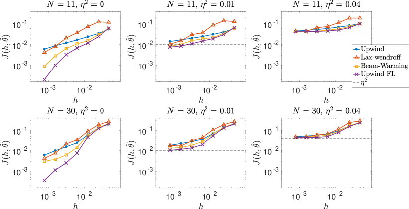
Figure 2: Plots of $J_{OLS}^{M,N}(h,\hat{\theta}_{OLS}^{M,N}(\boldsymbol{h}))$ for the four schemes considered with $\phi(x)=\phi_{d}(x)$. We depict the results for $N=11$ or 30 and $\eta^{2}=0,0.01,\text{ or }0.04$.

In Figure  2, we observe that $J^{M,N}(h,\hat{\theta}_{OLS}^{M,N}(h))$ appears to converge differently based on the numerical method used. To confirm this, we estimate the order of convergence of the numerical cost function by fitting the best-fit line between $\log\left(J^{M,N}(\vec{h},\hat{\theta}_{OLS}^{M,N}(\boldsymbol{h}))\right)$ and $\log(\boldsymbol{h})$. The slope of this line denotes the order of convergence for the numerical cost function, and we denote this calculation as $p_{J}$. We present some results for $\phi(x)=\phi_{d}(x)$ in Table  2. We observe that $p_{J}$ is about the same as $p$ for the upwind and Beam-Warming schemes and double the value of $p$ for the Lax-Wendroff Scheme when $\eta^{2}=0$. As $\eta^{2}$ increases, this value decreases. There is no apparent pattern between $p_{J}$ and $p$ for the upwind scheme with flux limiters. In the supporting material, we depict the values for $p_{J}$ for all data sets considered for $\phi(x)=\phi_{c}(x)$ in Table S1 and for $\phi(x)=\phi_{d}(x)$ in Table S3. For the continuous solutions when $\phi(x)=\phi_{c}(x),$ we observe that $p_{J}$ is often double the value of $p$. The order tends to decrease as $\eta$ increases for both continuous and discontinuous solutions, eventually reaching zero when experimental error dominates numerical error for all values in $\boldsymbol{h}$.

Numerical Method	$p$		$p_{J}$			$p_{\theta}$
			$0$	$4\times 10^{-2}$	$1$	$0$	$4\times 10^{-2}$	$1$
Upwind	0.5839	$11$	0.517	0.208	-0.002	0.360	0.446	0.406
		30	0.612	0.226	0.040	0.515	0.447	0.608
Lax-Wendroff	0.4737	$11$	0.966	0.490	-0.011	0.463	0.680	0.355
		30	0.878	0.387	0.062	1.023	0.523	0.213
Beam-Warming	.7876	$11$	0.785	0.367	0.000	0.769	0.525	-0.077
		30	0.987	0.441	0.040	0.380	0.518	0.303
Upwind FL	.9570	11	1.285	0.409	-0.020	0.582	0.510	-0.199
		30	1.338	0.505	0.037	0.189	0.523	-0.538

Table 2: Table of computed numerical and statistical orders of convergence for each data set when computed with different numerical methods for $\phi(x)=\phi_{d}(x)$. The variable $p$ denotes the computed order of numerical accuracy, $p_{J}$ denotes the computed order of convergence for the numerical cost function, and $p_{\theta}$ denotes the computed order of convergence for $\|\hat{\theta}_{OLS}^{M,N}(h)-\theta_{0}\|_{2}$.

It is at first puzzling that $p_{J}\approx 2p$ for the Lax-Wendroff method when $\phi(x)=\phi_{d}(x)$, yet $p_{J}\approx p$ for the upwind and Beam-Warming methods. This behavior can be explained, however, by looking at the terms A-F from Equation (9) that result from these different computations. In Figures S14-S17 in the supporting material, we depict the components A through F against $J_{OLS}^{M,N}(\boldsymbol{h},\hat{\theta}_{OLs}^{M,N}(\boldsymbol{h}))$ for all data sets and for all numerical schemes used. For the upwind scheme, the $\mathcal{O}(h^{p})$ term $B$ is on the same order of magnitude as $J_{OLS}^{M,N}(h,\hat{\theta}_{OLs}^{M,N}(h))$, which causes $p_{J}\approx p$. For the Lax-Wendroff scheme, the $\mathcal{O}(h^{2p})$ term $C$ tends to dominate the numerical cost function as $h$ decreases. This different behavior of terms A through F for different numerical methods is a likely explanation for the different $p_{J}/p$ ratios computed for our numerical methods. We depict these plots of A-F for all schemes considered in the supporting material in Figures S4-S7 for $\phi(x)=\phi_{c}(x)$.

4.3 Behavior of the Numerical OLS Estimator

In Figure  3, we depict plots of $\|\hat{\theta}_{OLS}^{M,N}(\boldsymbol{h})-\theta_{0}\|_{2}$ against $\boldsymbol{h}$ for $\phi(x)=\phi_{d}(x)$. The “Upwind auto” estimates modify cost function computation and will be discussed later in Section  5.1 with our residual analysis. In this figure, we observe that it is hard to predict which scheme will estimate $\theta_{0}$ best. For example, the Beam-Warming and upwind with flux limiter schemes tend to estimate $\theta_{0}$ best out of all methods considered. The Lax-Wendroff method also provides the best estimate of $\theta_{0}$ in some cases, however, but its accuracy is unpredictable. Recall from Figure  4.1 that the Lax-Wendroff method computes very dispersive $u(t,x;h,\theta)$ profiles. These dispersive oscillations are a likely explanation for the somewhat unpredictable $\hat{\theta}_{OLS}^{M,N}(h)$ estimates for this method. It is possible that numerical simulations that are computed with parameter vectors close to $\theta_{0}$ cause oscillations that prevent the numerical approximation from matching the data closely, whereas numerical simulations that are computed at vectors farther from $\theta_{0}$ cause oscillations that help the numerical approximation match the given data points. We depict plots of $\|\hat{\theta}_{OLS}^{M,N}(\boldsymbol{h})-\theta_{0}\|_{2}$ for all data sets considered in the supporting material in Figure S3 for $\phi(x)=\phi_{c}(x)$ and in Figure S13 for $\phi(x)=\phi_{d}(x).$ These figures show that the Beam-Warming and Lax-Wendroff schemes often do best for $\phi(x)=\phi_{c}(x)$ and confirm that the best method is hard to declare for $\phi(x)=\phi_{d}(x).$

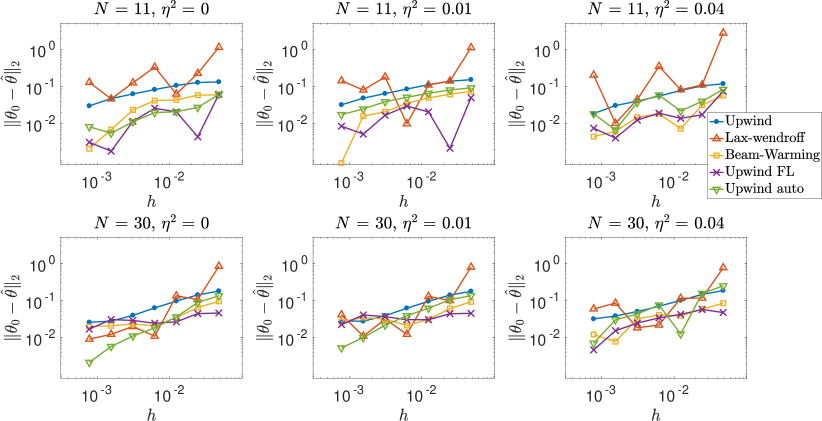
Figure 3: Plots of $\|\theta_{0}-\hat{\theta}_{OLS}^{M,N}(\boldsymbol{h})\|_{2}$ for the four schemes considered with $\phi(x)=\phi_{d}(x)$. We depict the results for $N=11$ or 30 and $\eta^{2}=0,0.01,$ or 0.04.

We depict a representative selection of computed orders of convergence for $\|\hat{\theta}_{OLS}^{M,N}(\boldsymbol{h})-\theta_{0}\|_{2}$ (denoted as $p_{\theta}$) in Table  2. All results for $\phi(x)=\phi_{d}(x)$ are included in Table S4 in the supporting material. We observe that $p_{\theta}\approx p$ for the upwind and Beam-Warming schemes and $p_{\theta}\approx p$ or $p_{\theta}\approx 2p$ for the Lax-Wendroff Scheme when $\eta^{2}=0$. There is no apparent pattern between $p_{\theta}$ and $p$ for the upwind scheme with flux limiters, although often $p_{\theta}\approx 0$ for this method. Recall from Corollary  2 that we expect $\hat{\theta}_{OLS}^{M,N}(h)$ to asymptotically behave as a random variable with mean $\theta_{0}$ and a variance that converges as $\mathcal{O}(h^{p}).$ This may explain why many estimates are converging with $p_{\theta}\approx p$: they converge as their variance. It is not clear why $p_{\theta}\approx 2p$ for some results with the Lax-Wendroff method. In the supporting material, we depict the values for $p_{\theta}$ for all data sets considered for $\phi(x)=\phi_{c}(x)$ in Table S2 and see that $p_{\theta}\approx p$ for all numerical methods.

5 Residual Analysis and Confidence Intervals

In Figure  4, We depict the residuals for the upwind method, along with $u(t_{i},x_{j};h,\hat{\theta}_{OLS}^{M,N}(h))$, and observe that local correlations in residual values arise near the point of discontinuity. Accordingly, in this section, we will explore how using an autocorrelative statistical model can improve uncertainty quantification for our inverse problem when using the first-order upwind method. In Section  5.1, we will use residual analysis to derive this statistical model. We will demonstrate how this statistical model can improve confidence interval computation in Section  5.2.

5.1 Residual Analysis

The statistical model describes how the underlying mathematical model is observed through experimental data. Residuals can be used to help practitioners ascertain the underlying statistical model of their data  [3]. If numerical error is prevalent in a practitioner’s computation, then it is interesting to consider how numerical error propagates in residual computation. Here we will develop an autocorrelative statistical model to describe how numerical error propagates in the inverse problem when using the upwind method for numerical computation when $\phi(x)=\phi_{d}(x)$.

We define the residual at the point $(t_{i},x_{j})$ as

$$r_{i,j}=u(t_{i},x_{j};h,\hat{\theta}_{OLS}^{M,N}(h))-y_{ij}.$$

By minimizing the numerical OLS cost function from Equation (6) in our inverse problem methodology, we are implicitly assuming that each residual value is independent and identically distributed (i.i.d.), which we expect to be true based on our statistical model in Equation (3). We observe from Figure  4 that the residuals are neither independent nor identically distributed: they are largest near the front location and are correlated with their neighboring residual values. Numerical diffusion from the upwind method is the likely explanation for these residual patterns. It smoothens the numerical solution near the point of discontinuity, which causes the computation to fall below the analytical solution at values just left to the point of discontinuity and to rise above the analytical solution at values to the right of the point of discontinuity. The correlation between neighboring data points indicates that an autocorrelative statistical model may be suitable to describe this behavior.

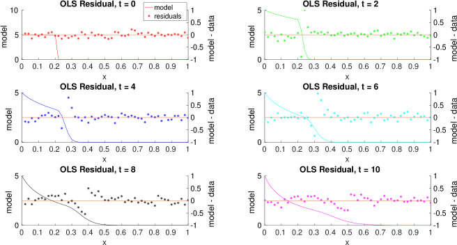
Figure 4: Plots of $r_{i,j}$ (dots) against simulations of $u(x,t;h,\hat{\theta})$ for the upwind method with $h=1/(10\times 2^{4})$ for $\eta=0.1$ and $\phi(x)=\phi_{d}(x)$.

To quantify the autocorrelated error that arises from numerical diffusion in this method, we assume the first order autocorrelation structure from  [11, $\S$ 6.2.3] arises. To illustrate this structure, assume that the point of discontinuity occurs at the location $x=x_{d_{i}}$ at $t=t_{i}$. This method assumes that the residual values to the right of $x_{d_{i}}$ at the fixed time $t_{i}$ will satisfy

$$r_{i,d_{i}} =\dfrac{1}{\sqrt{1-\gamma_{i,+}^{2}}}\epsilon_{i,d_{i}}$$

$$r_{i,d_{i+1}} =\gamma_{i}^{+}r_{i,d_{i}}+\epsilon_{i,d_{i+1}}$$

$$r_{i,d_{i+2}} =\gamma_{i}^{+}r_{i,d_{i+1}}+\epsilon_{i,d_{i+2}}$$

$$\vdots$$

$$r_{iN} =\gamma_{i}^{+}r_{iN-1}+\epsilon_{iN}$$ (10)

for $\epsilon_{i,j}\stackrel{{\scriptstyle i.i.d.}}{{\sim}}\mathcal{N}(0,\eta^{2})$ and $\gamma_{i}^{+}$ is the autocorrelation constant at time $t_{i}$ for points to the right of $x_{d}$. If we let $\vec{r}_{i,+}$ and $\vec{\epsilon}_{i,+}$ denote the $(N-d_{i}+1)\times 1$ vector of spatial residual values and Gaussian noise terms to the right of (and including) $x_{d}$ at time $t=t_{i}$, then

$$R_{i}^{+}\vec{r}_{i,+}=\vec{\epsilon}_{i,+}$$ (11)

for

$$R_{i}^{+}=\left[\begin{array}[]{ccccc}\sqrt{1-(\gamma_{i}^{+})^{2}}&0&0&\dots&0\\ -\gamma_{i}^{+}&1&0&&0\\ 0&-\gamma_{i}^{+}&\ddots&\ddots&\vdots\\ \vdots&&\ddots&1&0\\ 0&0&\dots&-\gamma_{i}^{+}&1\end{array}\right].$$

By combining Equations (3) and (11), we see that

$$R_{i}^{+}\vec{r}_{i,+}\stackrel{{\scriptstyle i.i.d.}}{{\sim}}\mathcal{N}(0,\eta^{2}I).$$ (12)

We will define an analogous statistical model at time $t_{i}$ for the points to the left of $x=x_{d}$ with rate of autocorrelation $\gamma_{i}^{-}$ and matrix $R_{i}^{-}$ so that $R_{i}=\text{diag}(\{R_{i}^{-},R_{i}^{+}\})$ and $R_{i}\vec{r}_{i}\stackrel{{\scriptstyle i.i.d.}}{{\sim}}\mathcal{N}(0,\eta^{2})$ for $\vec{r}_{i}$ denoting the $N\times 1$ vector of residuals at time $t_{i}$. Ultimately, we have

$$R\vec{r}\ \stackrel{{\scriptstyle i.i.d.}}{{\sim}}\mathcal{N}(0,\eta^{2}I)$$ (13)

for $R=\text{diag}\left(\{R_{i}\}_{i=1}^{M}\right)$ when $U(h,\theta)$ is used to approximate $U_{0}(\theta)$.

To estimate $\theta_{0}$ and quantify numerical error with an autocorrelation model, we perform the following two-stage estimation routine for a data set with a given step size, $h$ (taken from  [11, $\S$ 6.2.3], with modification):

1. Fit the model by finding the estimator, $\hat{\theta}_{OLS}^{M,N}(h)$, that minimizes Equation (6). 2. Compute the corresponding OLS residuals, $\vec{r},$ and estimate $\gamma_{i}$ and $\gamma_{i,b}$ using the formulas $\displaystyle\gamma_{i}^{+}=\dfrac{\sum_{j=d_{i}}^{N-1}r_{i,j}r_{i,j+1}}{\sum_{j=d_{i}}^{N-1}r_{i,j}^{2}},\ \gamma_{i}^{-}=\dfrac{\sum_{j=1}^{d_{i}-1}r_{i,j}r_{i,j+1}}{\sum_{j=1}^{d_{i}-1}r_{i,j}^{2}},\ i=1,...,M$ 3. Fit the model by find the estimator, $\hat{\theta}_{auto}^{M,N}(h)$, that minimizes $\displaystyle J_{auto}^{M,N}(h,\theta)=\dfrac{1}{MN}\vec{r}^{T}V^{-1}\vec{r},\ V^{-1}=R^{T}R.$

We performed this autocorrelation optimization method for the upwind method and depict the resulting modified residuals, $R\vec{r}$, in Figure  5. Here we see that the modified residuals do appear i.i.d., suggesting that the autocorrelation method is capable of accurately correcting residual computations when error from numerical diffusion arises. We only show the results for one data set here, but others exhibit similar results.

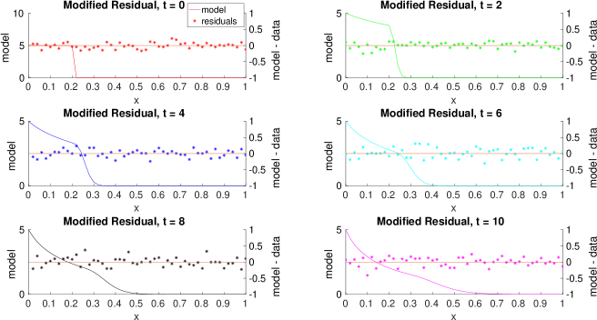
Figure 5: Plots of modified residuals (dots) against simulations of $u(x,t;h,\hat{\theta})$ for the upwind method with $h=1/(10\times 2^{4})$ with $\eta=0.1$ and $\phi(x)=\phi_{d}(x)$.

The goal of the autocorrelative statistical model is not only to determine the underlying statistical model, but also to improve estimation of $\theta_{0}$ by doing so. In Figure  3, we depict some plots of $\|\hat{\theta}_{auto}^{M,N}(\boldsymbol{h})-\theta_{0}\|_{2}$. In Figure S13 in the supporting material, we show this for all data sets considered. Here we see that $\hat{\theta}_{auto}^{M,N}(h)$ is improved over $\hat{\theta}_{OLS}^{M,N}(h)$ for the upwind method for many data sets and step size values. This method even outperforms the Beam-Warming, Lax-Wendroff, and upwind scheme with flux limiters in several cases. For larger values of $\eta^{2},$ estimation of $\theta_{0}$ was not significantly improved with the autocorrelation estimation routine, suggesting that the autocorrelation scheme cannot improve estimation when there is significantly more experimental error present than numerical error.

5.2 Confidence Interval Computation

If for some matrix, $Q$, we let the estimator, $\hat{\theta}^{M,N}$, satisfy

$$\hat{\theta}^{M,N}(h)=\arg\min_{\theta\in Q_{ad}}\dfrac{1}{MN}\vec{r}^{T}Q^{T}Q\vec{r},$$

and assume that the residuals satisfy $(Q\vec{r})_{i}\stackrel{{\scriptstyle i.i.d.}}{{\sim}}\mathcal{N}(0,\eta^{2})$, then asymptotically as $M,N\rightarrow\infty,$

$$\hat{\theta}^{M,N}(h)\sim\mathcal{N}(\theta_{0},H_{0}^{M,N})\approx\mathcal{N}\left(\theta_{0},\eta^{2}\left[\left[Q\nabla U_{0}(\theta_{0})\right]^{T}\left[Q\nabla U_{0}(\theta_{0})\right]\right]^{-1}\right).$$

See  [11, Theorem 2.1] for more details. Observe that $P=I$ when minimizing the OLS cost function and $P=R$ when minimizing the autocorrelation cost function described in Section  5.1. From this, we can show that the $(1-a)100\%$ confidence interval for the $k^{\text{th}}$ component of $\theta_{0}$ is given by the interval

$$\hat{\theta}_{k}^{M,N} \pm SE_{k}(\hat{\theta}^{M,N})t_{1-\nicefrac{{a}}{{2}}}^{MN-k_{\theta}},$$

$$\text{for }SE_{k}(\hat{\theta}) =\sqrt{\hat{\eta}^{2}\hat{H}_{kk}(\hat{\theta})},$$

$$\text{where }\hat{H}(\hat{\theta}) =\left[\left(Q\nabla U_{0}(\theta_{0})\right)^{T}\left(Q\nabla U_{0}(\theta_{0})\right)\right]^{-1}$$

$$\text{and }\hat{\eta}^{2} =\dfrac{1}{MN-k_{\theta}}\vec{r}^{T}Q^{T}Q\vec{r}$$ (14)

where $t_{1-\nicefrac{{a}}{{2}}}^{n}$ is the value such that $P(T\geq t_{1-\nicefrac{{a}}{{2}}}^{n})=\nicefrac{{a}}{{2}}$ if $T$ is a sample from the student’s t-distribution with $n$ degrees of freedom.

In Figure  6, we depict several 95% OLS confidence intervals that have been computed with the upwind method for $\phi(x)=\phi_{d}(x)$. The blue (red) confidence regions have been computed with large (small) values of $h$. We observe that the confidence intervals can enclose $\theta_{0}$ well for $N=11$ with the finest grid computations, but often miss $\theta_{0}$ for $N=30$. Note that these confidence intervals for $N=30$ are close to $\theta_{0},$ yet their small areas prevent them from actually enclosing $\theta_{0}$. In the supporting material, we depict the confidence intervals for all data sets considered for $\phi(x)=\phi_{c}(x)$ in Figures S8-S11. The upwind scheme struggles in these confidence intervals, but the Beam-Warming and Lax-Wendroff schemes can enclose $\theta_{0}$ reliably. In the supporting material, we depict the confidence intervals for all data sets considered for $\phi(x)=\phi_{d}(x)$ in Figures S18-S21. The confidence regions for the Lax-Wendroff, Beam-Warming, and upwind with flux limiters methods can all capture $\theta_{0}$ for $N=11,$ but struggle for $N=30$ and 51. These confidence intervals approach $\theta_{0}$ as $h\rightarrow 0$, but their areas are too small to capture $\theta_{0}$.

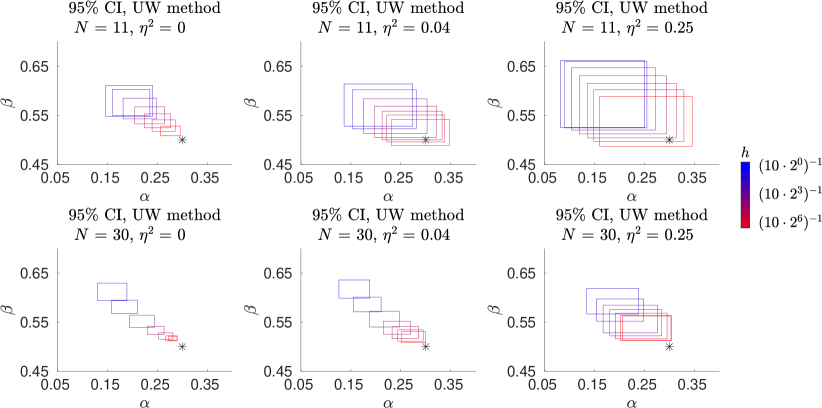
Figure 6: 95% OLS confidence intervals for $\theta=(\alpha,\beta)^{T}$ using Equation (14) with an upwind scheme and $\phi(x)=\phi_{d}(x)$ . The asterisk denotes $\theta_{0},$ and computations were done with a smaller value of $h$ as the confidence region color changes from blue to red.

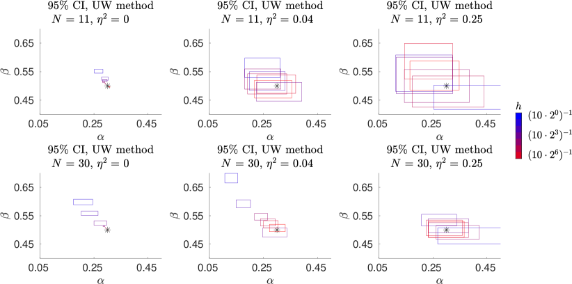
Figure 7: 95% autocorrelative confidence intervals for $\theta=(\alpha,\beta)^{T}$ using Equation (14) with an upwind scheme and $\phi(x)=\phi_{d}(x)$. The asterisk denotes $\theta_{0},$ and computations were done with a smaller value of $h$ as the confidence region color changes from blue to red.

Figure  7 depicts the calculated 95% confidence intervals for $\theta=(\alpha,\beta)^{T}$ when using the autocorrelative statistical model from Section  5.1 with the upwind method and $\phi(x)=\phi_{d}(x)$. We see that these confidence regions are an improvement over the OLS confidence intervals, as the confidence intervals enclose $\theta_{0}$ for most values of $h$ when $N=11$ and $\eta^{2}\neq 0,$ and the confidence intervals do enclose $\theta_{0}$ for smaller values of $h$ when $N=30$ and $\eta^{2}\neq 0.$ The autocorrelative confidence intervals are depicted for all data sets in the supporting material in Figure S22. In general, the method can significantly improve confidence interval computation for the upwind scheme, but still struggles when $N=51$.

6 Suggestions for practitioners

Based on our results, we suggest some strategies for practitioners in this section to improve their inverse problem methodologies. The conclusions from this section are summarized in Table  6.

If one is concerned with minimizing $J_{OLS}^{M,N}(h,\hat{\theta}_{OLS}^{M,N}(h))$ (and in turn inferring $\eta^{2}$, the variance of the experimental error in their data), one can determine if they have reached the true minimum value by performing the inverse problem discussed here for multiple values of the grid size, $h$. If the computed cost function decreases as $h$ decreases, then $J_{OLS}^{M,N}(h,\hat{\theta}_{OLS}^{M,N}(h))$ is likely larger than $\eta^{2}$ and not a reliable estimate. In this case, computation of $J_{OLS}^{M,N}(h,\hat{\theta}_{OLS}^{M,N}(h))$ can be improved with further grid refinement or by quantifying the effects of numerical error through a statistical model, similar to our analysis in Section  5. If the order of the numerical cost function appears to be zero, which can be confirmed by finding the best-fit line to $\ln\left(J_{OLS}^{M,N}(\boldsymbol{h},\hat{\theta}_{OLS}^{M,N}(\boldsymbol{h}))\right)$ against $\ln(\boldsymbol{h})$, then the practitioner can be confident that $J_{OLS}^{M,N}(h,\hat{\theta}_{OLS}^{M,N}(h))\approx\eta^{2},$ especially if $M,N$ are large. More data points can also make the computation of $J_{OLS}^{M,N}(h,\hat{\theta}_{OLS}^{M,N}(h))$ as an estimate of $\eta^{2}$ more reliable.

We observe in Figure  3 that the choice of step size, $h$, and numerical method can lead to different parameter estimate values. Accurate parameter estimation is a crucial element in understanding the scientific system under consideration. To determine which numerical method can most accurately estimate $\theta_{0}$ for a given $h$, a practitioner may use an artificially-generated data set, similar to what we’ve done in this study. This data set should resemble the true data as much as possible: it should have the same number of data points, be parameterized by some rough estimate of $\theta_{0}$ (such as $\hat{\theta}_{OLS}^{M,N}(h)$ for some value of $h$), and have the variance of the data points be an estimate of $\eta^{2}$ (such as $J_{OLS}^{M,N}(h,\hat{\theta}_{OLS}^{M,N}(h))$ for some value of $h$). If an analytical solution is not available for this data generation, then a very small value of $h$ could be used to generate the data, and a very accurate numerical method (such as the upwind scheme with flux limiters) should be used. One should be mindful that the choice of numerical method may skew their results. With this data set, determine which numerical method can most accurately estimate the parameter value used to parameterize the artificial data. This method should be used to fit the experimental data and estimate $\theta_{0}$.

Using a smaller value of $h$ will often not be a practical solution as a means to improve inverse problem results. We saw in this work that two alterations can be incorporated with the upwind method to improve its results: the use of flux limiters in computation or an autocorrelative statistical model. Both of these strategies have their advantages and disadvantages. The upwind scheme with flux limiters yields a very accurate simulation profile (as seen in Figure  4.1), but does increase the computation time because the spatial gradient has to be estimated at each time iteration. The autocorrelative statistical model is not computationally expensive; it should only double the computation time of the inverse problem (one round of OLS optimization followed by another round of autocorrelative optimization). We see in Figure S22 in the supporting material that this autocorrelative statistical model can successfully improve estimate values of $\theta_{0}$ when $\eta^{2}$ is small. Both of these alterations were also only effective for $\phi(x)=\phi_{d}(x);$ we can not recommend one use these methods when the model solution is continuous.

Lastly, we saw that both the incorporation of flux limiters and the autocorrelative statistical method could enhance confidence interval computation in Section  5.2. The biggest factor in preventing accurate confidence interval computation in this study is large numbers of data points. All methods struggled to enclose $\theta_{0}$ for $N=51$, which is likely because these confidence intervals have very small areas. If a practitioner is concerned with accurate confidence interval computation, then we may suggest checking that they can accurately enclose $\theta_{0}$ for artificial data sets with the same number of points as their data sets. If not, they should consider subsets of their data that will compute wider confidence regions that can capture $\theta_{0}$ more reliably. The autocorrelative statistical model and the incorporation of flux limiters are also excellent methods to improve confidence interval computation, as seen in Figures S21 and S22 in the supporting material.

Task	To do	Conclusions/Notes
Improve		If $J_{OLS}(\hat{\theta},\boldsymbol{h})$ does not change, the minimum has likely been reached.
minimization	compute $J_{OLS}(\hat{\theta},h)$	If $J_{OLS}(\hat{\theta},\boldsymbol{h})$ is decreasing with $h$, computation can be improved with
of $J_{OLS}(\hat{\theta},h)$	for several values of $h$	smaller values of $h$ or by using a statistical model to account for
		numerical error.
Determine best	Perform IP on	Choose the method that can best predict the value of $\theta$ that
numerical method	artificially-generated data	generated the data. If no analytical solution exists, keep in mind
	with multiple methods	that the method used in generating data will bias results.
Improve results	1. Perform more accurate	1. Note that flux limiters will also increase the computation time.
without	computation (e.g., flux limiters)	2. Note that the autocorrelative statistical model worked best
decreasing $h$	2. Use statistical model	when $\eta^{2}$ was small.
	to incorporate numerical error	Both of these strategies work well for discontinuous solutions.
	1. Perform IP on	1. Reduce number of data points to a number
	artificially-generated data	where CI computations reliably enclosed $\theta_{0}$
Improve CI	with fewer data points.	for artificially generated data sets.
computation	2. Use statistical model	2. Note that this only works for methods that
	to incorporate numerical error	admit numerical diffusion.
	3. Use flux limiters	3. Will increase computation time.

Summary of strategies to help practitioners improve the results of their inverse problem methodologies. The “Task” column denotes a task that one may wish to carry out. The “To do” column suggests some strategies to perform the desired task. The “Conclusions/Notes” column provides guidelines on how to interpret the different results one may find, as well as notes to keep in mind when making final conclusions. The abbreviations in the table include: $\hat{\theta}=\hat{\theta}_{OLS}^{M,N}(h),$ IP = inverse problem, and CI = confidence interval.

7 Discussion and Future Work

Numerical approximations for advection-dominated processes are a known challenge in the sciences  [7, 13], and the precise effects of numerical error on an inverse problem have not been investigated thoroughly. In this document, we fit various numerical schemes with varying orders of convergence to artificial data with different numbers of data points and error levels. We use a numerical cost function in a similar vein to that in  [2] to show how the convergence of the cost function depends on the orders of convergence of the numerical scheme used. We also determined the asymptotic distribution of the parameter estimator in the presence of approximation error. In general, the second order methods outperform the first order upwind methods in computing the cost function and in parameter estimation, as one would would expect. There are ways to improve results with this first order method, however, including the use of flux limiters or an autocorrelative statistical model. This autocorrelative statistical model describes how numerical error propagates in the inverse problem and in turn improve parameter estimation and confidence interval computation. The incorporation of flux limiters into computation with the upwind method improves computation accuracy as well as parameter estimation.

There are some aspects of this study that we have left for future work. In Figure  8, we depict the OLS residuals when fitting the Lax-Wendroff method to the artificial data when $\phi(x)=\phi_{d}(x)$. Recall that the modified equation for this second order method is dispersive, so the leading error terms are composed of high-frequency modes from the initial condition propagating at different speeds. This set of residuals shows patterns that would be much more difficult to quantify than those presented in Section  5.1. Future work should include a careful analysis into how numerical error from this and other higher-order numerical methods influences the statistical model of the data. As we saw in this work, determining this influence would lead to improvements in parameter estimation and uncertainty quantification for these methods.

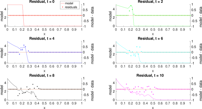
Figure 8: Plots of $r_{i,j}$ (dots) against simulations of $\vec{u}(x,t;h,\hat{\theta}_{OLS}^{M,N}(h))$ for the Lax-Wendroff method with $h=1/(10\times 2^{6})$ with $\eta=0$ for $\phi(x)=\phi_{d}(x).$

Appendix A Previous Theory of $\hat{\theta}_{OLS}^{M,N}$

In this Section, we state part of Theorem 2.1 from  [11].

Theorem.

Given that $\mathcal{\vec{\epsilon}\sim\mathcal{N}}(0,\eta^{2}I)$ and $u_{0}(t,x;\theta)$ is sufficiently smooth with respect to $\theta,$ then we have the asymptotic distribution for $\theta_{OLS}^{M,N}$ as $M,N\rightarrow\infty$ given by

$$\theta_{OLS}^{M,N}\sim\mathcal{N}(\theta_{0},\eta^{2}V),\ V=(\nabla_{\theta}U_{0}(\theta_{0})^{T}\nabla_{\theta}U_{0}(\theta_{0}))^{-1}.$$

Appendix B Convergence of the terms of $J_{OLS}^{M,N}(h,\theta)$

Here we discuss the asymptotic properties of $J_{OLS}^{M,N}(h,\theta)$. We begin with the limits as $h\rightarrow 0$ in Section  B.1 and as $M,N\rightarrow\infty$ in  B.2.

For brevity, we denote $\hat{\theta}_{OLS}^{M,N}(h)$ as $\hat{\theta}$ for the rest of this section.

Note that  [2] includes more assumptions than those provided in this study, but they are already satisfied by Equations (1) or (3). Assumption (A1) here is a modification of (A3) in  [2] to include convergence of $L^{1}$ functions.

B.1 Limits as $h\rightarrow 0$

Here we provide the proof to Lemma  3.

Proof.

Note that our definition for the numerical order of convergence gives that

$$\|\vec{U}_{0}(\hat{\theta})-\vec{U}(h,\hat{\theta})\|_{1}=\mathcal{O}(h^{p}).$$

Term A is independent of $h$, so it acts as $\mathcal{O}(1)$.

Term $B$ is given as

$$B=\dfrac{1}{MN}\sum_{i,j=1}^{M,N}[u_{0}(t_{i},x_{j};\theta_{0})-u_{0}(t_{i},x_{j};\hat{\theta})]^{2}.$$

As $h\rightarrow 0$ and $\hat{\theta}$ approaches $\theta_{0}$ (assuming that there are enough data points used for this to occur). We can Taylor expand about $\theta_{0}$ and find

$$B\approx\dfrac{1}{MN}\sum_{i,j=1}^{M,N}[\nabla_{\theta}U_{0}(t_{i},x_{j};\theta_{0})[\hat{\theta}-\theta_{0}]]^{2}.$$

Note that $\nabla_{\theta}U_{0}(t_{i},x_{j};\theta_{0})$ is independent of $h$, but from Corollary  2, we have that $\hat{\theta}\sim\mathcal{N}(\theta_{0},V_{h})$ where each entry of $V_{h}$ converges to its corresponding entry of $V$ as $\mathcal{O}(h^{p}).$ Each term being summed is thus a random variable with mean independent of $h$ and variance acting as $\mathcal{O}(h^{2p}).$ We thus conclude that this random variable has standard deviation $\mathcal{O}(h^{p})$. Thus $B$ converges as $\mathcal{O}(h^{p})$.

Term $C$ is given by

$$C=\dfrac{1}{MN}\sum_{i,j=1}^{M,N}[u_{0}(t_{i},x_{j};\hat{\theta})-u(t_{i},x_{j};h,\hat{\theta})]^{2},$$

which may also be written in terms of the Euclidean vector norm, from where we can then use equivalence of finite-dimensional norms to show that it will converge as $\mathcal{O}(h^{2p})$ by assuming that $\hat{\theta}$ is in the compact space, $\Theta_{ad}$:

$$C =\dfrac{1}{MN}\|\vec{U}_{0}(\hat{\theta})-\vec{U}(h,\hat{\theta})\|_{2}^{2}$$

$$\leq\dfrac{K^{2}}{MN}\|\vec{U}_{0}(\hat{\theta})-\vec{U}(h,\hat{\theta})\|_{1}^{2}=K_{C}h^{2p}\text{.}$$

Thus $C$ converges as $\mathcal{O}(h^{2p})$.

Term $D$ is given by

$$D=\dfrac{2}{MN}\sum_{i,j=1}^{M,N}\mathcal{\epsilon}_{i,j}(u_{0}(t_{i},x_{j};\theta_{0})-u_{0}(t_{i},x_{j};\hat{\theta}))$$

We begin with a Taylor expansion about $\theta_{0}$ to find

$$D\approx\dfrac{-2}{MN}\sum_{i,j=1}^{M,N}\epsilon_{i,j}(\nabla_{\theta}u_{0}(t_{i},x_{j};\theta_{0})(\hat{\theta}-\theta_{0})).$$

We then use the Cauchy-Schwarz Inequality to show

$$|D|\lesssim\sqrt{\dfrac{2}{MN}\left(\sum_{i,j=1}^{M,N}\epsilon_{i,j}^{2}\right)\dfrac{2}{MN}\left(\sum_{i,j=1}^{M,N}(\nabla_{\theta}U_{0}(\theta_{0})(\hat{\theta}-\theta_{0}))^{2}\right)}.$$

The first term on the right will be close to its finite mean of $\sqrt{2\eta^{2}}$ if $M,N$ are large by the law of large numbers (LLN). By Corollary  2, the second term on the right is equivalent to

$$\sqrt{\dfrac{2}{MN}\left(\sum_{i,j=1}^{M,N}(\nabla_{\theta}U_{0}(\theta_{0})\theta_{D})^{2}\right)},$$

where $\theta_{D}$ has a standard deviation that converges to $V$ as $\mathcal{O}(h^{p/2}).$ Everything else in this term is independent of $h$, so $D$ is a random variable with standard deviation converging as $\mathcal{O}(h^{p/2})$. Thus $D$ converges as $\mathcal{O}(h^{p/2})$.

The term $E$ is written as

$$E=\dfrac{2}{MN}\sum_{i,j=1}^{M,N}\mathcal{\epsilon}_{i,j}(u_{0}(t_{i},x_{j};\hat{\theta})-u(t_{i},x_{j};h,\hat{\theta})).$$

We can bound this term from above as $h\rightarrow 0$ as

$$|E| \leq\dfrac{2}{MN}\sqrt{\left(\sum_{i,j=1}^{M,N}\epsilon_{i,j}^{2}\right)\left(\sum_{i,j=1}^{M,N}\left|(u_{0}(x_{i},t_{j};\theta)-u(x_{i},t_{j};h,\theta))\right|^{2}\right)}$$

$$\leq\dfrac{2K}{MN}\sqrt{\left(\sum_{i,j=1}^{M,N}\epsilon_{i,j}^{2}\right)\left(\sum_{i,j=1}^{M,N}\left|(u_{0}(x_{i},t_{j};\theta)-u(x_{i},t_{j};h,\theta))\right|\right)^{2}}$$

$$=\mathcal{O}(h^{p})$$

where the first inequality is by the Cauchy-Schwarz inequality, the second is by the equivalence of finite-dimensional norms. The final approximation is from the LLN giving that the first term will converge to its finite mean for $M,N$ large and then our definition for the numerical order of convergence. Thus $E$ converges as $\mathcal{O}(h^{p})$.

Term F is written as

$$F=\dfrac{2}{MN}\sum_{i,j=1}^{M,N}\left[\left(u_{0}(x_{i},t_{j};\hat{\theta})-u(x_{i},t_{j};h,\hat{\theta})\right)\left(u_{0}(x_{i},t_{j};\theta_{0})-u_{0}(x_{i},t_{j};\hat{\theta})\right)\right].$$

Using the Cauchy-Schwarz Inequality, we find

$$|F| \leq\dfrac{2}{MN}\|\vec{U_{0}}(\hat{\theta})-\vec{U}(h,\hat{\theta})\|_{2}\|\vec{U}_{0}(\theta_{0})-\vec{U}_{0}(\hat{\theta})\|_{2}.$$

We then use the equivalence of norms and Taylor expansion about $\theta_{0}$ to find

$$|F| \lesssim\dfrac{2K}{MN}\|\vec{U_{0}}(\hat{\theta})-\vec{U}(h,\hat{\theta})\|_{1}\|\nabla U_{0}(\theta_{0})(\hat{\theta}-\theta_{0})\|_{2}.$$

The first term converges as $\mathcal{O}(h^{p})$ from our definition for the numerical order of convergence. The second term is a random variable with standard deviation converging as $\mathcal{O}(h^{p/2})$ from Corollary  2. Thus $F$ converges as $\mathcal{O}(h^{3p/2})$.

∎

B.2 Limits as $M,N\rightarrow\infty$

Here we provide the proof of Lemma  4.

Proof.

Note that $\epsilon_{i,j}^{2}$ is distributed as $\eta^{2}$ times a degree-1 chi-squared random variable. We thus observe that $A$ is distributed as $\nicefrac{{\eta^{2}}}{{MN}}$ times a degree-$MN$ chi-squared random variable, which has mean $\eta^{2}$ and variance $\nicefrac{{2\eta^{4}}}{{MN}}.$ By the classical Central Limit Theorem (CLT),

$$\sqrt{MN}(A-\eta^{2})\xrightarrow{D}\mathcal{N}(0,2\eta^{2})$$

as $M,N\rightarrow\infty$, where $\xrightarrow{D}$ denotes convergence in distribution. Thus $A$ converges as $\mathcal{O}\left(1/\sqrt{MN}\right)$.

Term B is the sum of the difference of the true solution squared when computed at $\theta_{0}$ and $\theta$. From assumption (A1),

$$B(\hat{\theta}) =\dfrac{1}{MN}\sum_{i,j=1}^{M,N}[u_{0}(t_{i},x_{j};\theta_{0})-u_{0}(t_{i},x_{j};\hat{\theta})]^{2}\rightarrow J^{*}(\hat{\theta}).$$

$\text{as }M,N\rightarrow\infty$ by (A1). This convergence is identical to a first order Riemann sum. Thus $B$ converges with order $\mathcal{O}\left(1/(MN)\right)$.

Term $C$ is given by

$$C=\dfrac{1}{MN}\sum_{i,j=1}^{M,N}[u_{0}(t_{i},x_{j};\hat{\theta})-u(t_{i},x_{j};h,\hat{\theta})]^{2}.$$

We assume $\hat{\theta}$ stays within $Q_{ad}$ and use our Definition for the order of convergence to find that

$$C\approx\dfrac{1}{MN}\sum_{i,j=1}^{M,N}[w(t_{i},x_{j};h)h^{p}]^{2}=\mathcal{O}(h^{2p}),$$

Thus $C$ is independent of $M,N$.

Term D is written as

$$D=\dfrac{2}{MN}\sum_{i,j=1}^{M,N}\epsilon_{i,j}(u_{0}(t_{i},x_{j};\theta_{0})-u_{0}(t_{i},x_{j};\hat{\theta})).$$

$u_{0}(t,x;\theta)$ is bounded below by 0 and above by 1, so we can bound this term as

$$\dfrac{-2}{MN}\sum_{i,j=1}^{M,N}\epsilon_{i,j}\leq D\leq\dfrac{2}{MN}\sum_{i,j=1}^{M,N}\epsilon_{i,j}.$$

By the CLT, both of these bounds will converge in distribution to zero with order $\mathcal{O}(1/\sqrt{MN})$. Thus $D$ converges as $\mathcal{O}(1/\sqrt{MN}).$

Term $E$ is written as

$$E=\dfrac{2}{MN}\sum_{i,j=1}^{M,N}\epsilon_{i,j}(u_{0}(t_{i},x_{j};\theta)-u(x_{i},t_{j};h,\theta)).$$

We assume $\hat{\theta}$ stays within $Q_{ad}$ and use our definition for the order of convergence to find that

$$E\approx\dfrac{2}{MN}\sum_{i,j=1}^{M,N}\epsilon_{i,j}w(t_{i},x_{j};h)h^{p},$$

so that

$$-\dfrac{2h^{p}}{MN}\sum_{i,j=1}^{M,N}\epsilon_{i,j}\lesssim E\lesssim\dfrac{2h^{p}}{MN}\sum_{i,j=1}^{M,N}\epsilon_{i,j},$$

which shows that $E$ will converge in distribution to zero with order $\mathcal{O}(1/\sqrt{MN})$ as $M,N\rightarrow\infty$ by the CLT. Thus $E$ converges as $\mathcal{O}(1/\sqrt{MN})$.

Term F is written as

$$F=\dfrac{2}{MN}\sum_{i,j=1}^{M,N}\left[\left(u_{0}(x_{i},t_{j};\hat{\theta})-u(x_{i},t_{j};h,\hat{\theta})\right)\left(u_{0}(x_{i},t_{j};\theta_{0})-u_{0}(x_{i},t_{j};\hat{\theta})\right)\right].$$

If we assume that $\hat{\theta}$ remains in $Q_{ad}$ then we can use our definition for the order of convergence and the boundedness of $w(t,x;h)$ to show that

$$\dfrac{-2h^{p}}{MN}\sum_{i,j=1}^{M,N}\left(u_{0}(x_{i},t_{j};\theta_{0})-u_{0}(x_{i},t_{j};\hat{\theta})\right)\leq F\leq\dfrac{2h^{p}}{MN}\sum_{i,j=1}^{M,N}\left(u_{0}(x_{i},t_{j};\theta_{0})-u_{0}(x_{i},t_{j};\hat{\theta})\right).$$

If we define

$$J^{1}(\theta)=\int_{X}\int_{T}\left(u_{0}(x,t;\theta_{0})-u_{0}(x,t;\theta)\right)d\nu(t)d\chi(x),$$

then the sum in the above equation will converge to $\mathcal{O}(h^{p})J^{1}(\hat{\theta})$ as a first order Riemann sum. Note that we can bound this integral between -10 and 10. Thus $F$ converges as $\mathcal{O}(1/(MN))$ to a $\mathcal{O}(h^{p})$ term. ∎

References

- Ackleh and Thibodeaux [2008] Azmy Ackleh and Jeremy Thibodeaux. Parameter estimation in a structured erythropoiesis model. Mathematical Biosciences and Engineering, 5(4):601–616, October 2008. ISSN 1551-0018. doi: 10.3934/mbe.2008.5.601. URL http://www.aimsciences.org/journals/displayArticles.jsp?paperID=3701.
- Banks and Fitzpatrick [1990] H. T. Banks and B. G. Fitzpatrick. Statistical methods for model comparison in parameter estimation problems for distributed systems. Journal of Mathematical Biology, 28(5):501–527, September 1990. ISSN 0303-6812, 1432-1416. doi: 10.1007/BF00164161. URL http://link.springer.com/article/10.1007/BF00164161.
- Banks et al. [2012] H. T. Banks, Zachary R. Kenz, and W. C. Thompson. An Extension of RSS-based Model Comparison Tests for Weighted Least Squares. Technical report, North Carolina State University, Center for Research in Scientific Computation, Center for Quantitative Sciences in Biomedicine, August 2012.
- Banks and Tran [2009] H. Thomas Banks and Hien T. Tran. Mathematical and Experimental Modeling of Physical and Biological Processes. CRC Press, Boca Raton, FL, 2009.
- Higham [1996] Nicholas J. Higham. Accuracy and Stability of Numerical Algorithms. SIAM, Philadelphia, 1 edition, 1996.
- Holmes [2015] William R. Holmes. A practical guide to the Probability Density Approximation (PDA) with improved implementation and error characterization. Journal of Mathematical Psychology, 68-69:13–24, October 2015. ISSN 00222496. doi: 10.1016/j.jmp.2015.08.006. URL http://linkinghub.elsevier.com/retrieve/pii/S0022249615000541.
- Leonard [1991] B. P. Leonard. The ULTIMATE conservative difference scheme applied to unsteady one-dimensional advection. Computer Methods in Applied Mechanics and Engineering, 88(1):17–74, June 1991. ISSN 0045-7825. doi: 10.1016/0045-7825(91)90232-U. URL http://www.sciencedirect.com/science/article/pii/004578259190232U.
- LeVeque [2007] Randall J. LeVeque. Finite difference methods for ordinary and partial differential equations: steady-state and time-dependent problems. Society for Industrial and Applied Mathematics, Philadelphia, PA, 2007. ISBN 978-0-89871-629-0 0-89871-629-2.
- Nardini and Bortz [2018] John T. Nardini and D. M. Bortz. Investigation of a Structured Fisher’s Equation with Applications in Biochemistry. SIAM Journal on Applied Mathematics, (accepted), 2018.
- Randall J. Leveque [1992] Randall J. Leveque. Conservation Laws. Lectures in Mathematics. Birkhauser Verlag, 2 edition, 1992.
- Seber and Wild [1988] G. A. F. Seber and C. J. Wild. Nonlinear Regression. Wiley series in probability and statistics. Wiley, 1988.
- Sweby [1984] P. Sweby. High Resolution Schemes Using Flux Limiters for Hyperbolic Conservation Laws. SIAM Journal on Numerical Analysis, 21(5):995–1011, October 1984. ISSN 0036-1429. doi: 10.1137/0721062. URL http://epubs.siam.org/doi/abs/10.1137/0721062.
- Thackham et al. [2008] Jennifer A. Thackham, D. L. Sean McElwain, and Ian W. Turner. Computational Approaches to Solving Equations Arising from Wound Healing. Bulletin of Mathematical Biology, 71(1):211–246, December 2008. ISSN 0092-8240, 1522-9602. doi: 10.1007/s11538-008-9360-z. URL http://link.springer.com/article/10.1007/s11538-008-9360-z.
- Webb [2008] G. F. Webb. Population models structured by age, size, and spatial position. In Structured Population Models in Biology and Epidemiology, pages 1–49. Springer, 2008.
- Xue et al. [2010] Hongqi Xue, Hongyu Miao, and Hulin Wu. Sieve Estimation of Constant and Time-Varying Coefficients in Nonlinear Ordinary Differential Equation Models by Considering Both Numerical Error and Measurement Error. Annals of statistics, 38(4):2351–2387, January 2010. ISSN 0090-5364. URL http://www.ncbi.nlm.nih.gov/pmc/articles/PMC2995285/.