Variational Bayesian Reinforcement Learning with Regret Bounds

Abstract

In reinforcement learning the Q-values summarize the expected future rewards that the agent will attain. However, they cannot capture the epistemic uncertainty about those rewards. In this work we derive a new Bellman operator with associated fixed point we call the ‘knowledge values’. These K-values compress both the expected future rewards and the epistemic uncertainty into a single value, so that high uncertainty, high reward, or both, can yield high K-values. The key principle is to endow the agent with a risk-seeking utility function that is carefully tuned to balance exploration and exploitation. When the agent follows a Boltzmann policy over the K-values it yields a Bayes regret bound of $\tilde{O}(L\sqrt{SAT})$, where $L$ is the time horizon, $S$ is the total number of states, $A$ is the number of actions, and $T$ is the number of elapsed timesteps. We show deep connections of this approach to the soft-max and maximum-entropy strands of research in reinforcement learning.

1 Introduction and related work

In reinforcement learning (RL) an agent interacts with an environment in an episodic manner and attempts to maximize its return [54, 45]. In this work the environment is a Markov decision process (MDP) and we consider the Bayesian case where the agent has some prior information and as it gathers data it updates its posterior beliefs about the environment. In this setting the agent is faced with the choice of visiting well understood states or exploring the environment to determine the value of other states which might lead to a higher return. This trade-off is called the exploration-exploitation dilemma. One way to measure how well an agent balances this trade-off is a quantity called regret, which measures how sub-optimal the rewards the agent has received are so far, relative to the (unknown) optimal policy [12]. In the Bayesian case the natural quantity to consider is the Bayes regret, which is the expected regret under the agents prior information [17].

The optimal Bayesian policy can be formulated using belief states, but this is believed to be intractable for all but small problems [17]. Approximations to the optimal Bayesian policy exist, one of the most successful being Thompson sampling [53, 55] wherein the agent samples from the posterior over value functions and acts greedily with respect to that sample [38, 42, 27, 41]. It can be shown that this strategy yields both Bayesian and frequentist regret bounds under certain assumptions [3]. In practice, maintaining a posterior over value functions is intractable, and so instead the agent maintains the posterior over MDPs, and at each episode an MDP is sampled from this posterior, the value function for that sample is computed, and the policy acts greedily with respect to that value function. Due to the repeated sampling and computing of value functions this is practical only for small problems, though attempts have been made to extend it [37, 43].

Bayesian algorithms have the advantage of being able to incorporate prior information about the problem and, as we show in the numerical experiments, they tend to perform better than non-Bayesian approaches in practice [17, 51, 49]. Although typically Bayes regret bounds hold for any prior that satisfies the assumptions, the requirement that the prior over the MDP is known in advance is a disadvantage for Bayesian methods. One common concern is about performance degradation when the prior is misspecified. In this case it can be shown that the regret increases by a multiplicative factor related to the Radon-Nikodym derivative of the true prior with respect to the assumed prior [48, §3.1]. In other words, a Bayesian algorithm with sub-linear Bayes regret operating under a misspecified prior will still have sub-linear regret so long as the true prior is absolutely continuous with respect to the misspecified prior. Moreover, for any algorithm that satisfies a Bayes regret bound it is straightforward to derive a high-probability regret bound for any family of MDPs that has support under the prior, in a sense translating Bayes regret into frequentist regret; see [48, §3.1], [38, Appendix A] for details.

In this work we endow an agent with a particular epistemic risk-seeking utility function, where ‘epistemic risk’ refers to the Bayesian uncertainty that the agent has about the optimal value function of the MDP. In the context of RL, acting so as to maximize a risk-seeking utility function which assigns higher values to more uncertain actions is a form of optimism in the face of uncertainty, a well-known heuristic to encourage exploration [21, 5]. Any increasing convex function could be used as a risk-seeking utility, however, only the exponential utility function has a decomposition property which is required to derive a Bellman recursion [1, 44, 20, 46]. We call the fixed point of this Bellman operator the ‘K-values’ for knowledge since they compress the expected downstream reward and the downstream epistemic uncertainty at any state-action into a single quantity. A high K-value captures the fact that the state-action has a high expected Q-value or high uncertainty, or both. Following a Boltzmann policy over the K-values yields a practical algorithm that we call ‘K-learning’ which attains a Bayes regret upper bounded by $\tilde{O}(L\sqrt{SAT})$ where $L$ is the time horizon, $S$ is the total number of states, $A$ is the number of actions per state, and $T$ is the number of elapsed timesteps [11]. This regret bound matches the best known bound for Thompson sampling up to log factors [38] and is within a factor of $\sqrt{L}$ of the known information theoretic lower bound of $\Omega(\sqrt{LSAT})$ [23, Appendix D].

The update rule we derive is similar to that used in ‘soft’ Q-learning (so-called since the ‘hard’ max is replaced with a soft-max) [6, 16, 18, 30, 47]. These approaches are very closely related to maximum entropy reinforcement learning techniques which add an entropy regularization ‘bonus’ to prevent early convergence to deterministic policies and thereby heuristically encourage exploration [57, 59, 28, 35, 2, 25]. In our work the soft-max operator and entropy regularization arise naturally from the view of the agent as maximizing a risk-seeking exponential utility. Furthermore, in contrast to these other approaches, the entropy regularization is not a fixed hyper-parameter but something we explicitly control (or optimize for) in order to carefully trade-off exploration and exploitation.

The algorithm we derive in this work is model-based, i.e., requires estimating the full transition function for each state. There is a parallel strand of work deriving regret and complexity bounds for model-free algorithms, primarily based on extensions of Q-learning [23, 58, 26]. We do not make a detailed comparison between the two approaches here other than to highlight the advantage that model-free algorithms have both in terms of storage and in computational requirements. On the other hand, in the numerical experiments model-based approaches tend to outperform the model-free algorithms. We conjecture that an online, model-free version of K-learning with similar regret guarantees can be derived using tools developed by the model-free community. We leave exploring this to future work.

1.1 Summary of main results

• We consider an agent endowed an epistemic risk-seeking utility function and derive a new optimistic Bellman operator that incorporates the ‘value’ from epistemic uncertainty about the MDP. The new operator replaces the usual max operator with a soft-max and it incorporates a ‘bonus’ that depends on state-action visitation. In the limit of zero uncertainty the new operator reduces to the standard optimal Bellman operator.

• At each episode we solve the optimistic Bellman equation for the ‘K-values’ which represent the utility of a particular state and action. If the agent follows a Boltzmann policy over the K-values with a carefully chosen temperature schedule then it will enjoy a sub-linear Bayes regret bound.

• To the best of our knowledge this is the first work to show that soft-max operators and maximum entropy policies in RL can provably yield good performance as measured by Bayes regret. Similarly, we believe this is the first result deriving a Bayes regret bound for a Boltzmann policy in RL. This puts maximum entropy, soft-max operators, and Boltzmann exploration in a principled Bayesian context and shows that they are naturally derived from endowing the agent with an exponential utility function.

2 Markov decision processes

In a Markov decision process (MDP) an agent interacts with an environment in a series of episodes and attempts to maximize the cumulative reward. We model the environment as a finite state-action, time-inhomogeneous MDP given by the tuple $\mathcal{M}=\{\mathcal{S},\mathcal{A},R,P,L,\rho\}$, where $\mathcal{S}$ is the state-space, $\mathcal{A}$ is the action-space, $R_{l}(s,a)$ is a probability distribution over the rewards received by the agent at state $s$ taking action $a$ at timestep $l$, $P_{l}(s^{\prime}\mid s,a)\in[0,1]$ is the probability the agent will transition to state $s^{\prime}$ after taking action $a$ in state $s$ at timestep $l$, $L\in{\mathbb{N}}$ is the episode length, and $\rho$ is the initial state distribution. We assume that the state space can be decomposed layerwise as $\mathcal{S}=\mathcal{S}_{1}\cup\mathcal{S}_{2}\cup\ldots\cup\mathcal{S}_{L}$ and it has cardinality $|\mathcal{S}|=\sum_{l=1}^{L}|\mathcal{S}_{l}|=S$, and the cardinality of the action space is $|\mathcal{A}|=A$. Concretely, the initial state $s_{1}\in\mathcal{S}_{1}$ of the agent is sampled from $\rho$, then for timesteps $l=1,\ldots,L$ the agent is in state $s_{l}\in\mathcal{S}_{l}$, selects action $a_{l}\in\mathcal{A}$, receives reward $r_{l}\sim R_{l}(s_{l},a_{l})$ with mean $\mu_{l}(s_{l},a_{l})\in{\mathbb{R}}$ and transitions to the next state $s_{l+1}\in\mathcal{S}_{l+1}$ with probability $P_{l}(s_{l+1}\mid s_{l},a_{l})$. After timestep $L$ the episode terminates and the state is reset. We assume that at the beginning of learning the agent does not know the reward or transition probabilities and must learn about them by interacting with the environment. We consider the Bayesian case in which the mean reward $\mu$ and the transition probabilities $P$ are sampled from a known prior $\phi$. We assume that the agent knows $S$, $A$, $L$, and the reward noise distribution.

An agent following policy $\pi_{l}:\mathcal{S}_{l}\times\mathcal{A}\rightarrow[0,1]$ at state $s\in\mathcal{S}_{l}$ at time $l$ selects action $a$ with probability $\pi_{l}(s,a)$. The Bellman equation relates the value of actions taken at the current timestep to future returns through the Q-values and the associated value function [8], which for policy $\pi$ are denoted $Q_{l}^{\pi}\in{\mathbb{R}}^{|\mathcal{S}_{l}|\times A}$ and $V_{l}^{\pi}\in{\mathbb{R}}^{|\mathcal{S}_{l}|}$ for $l=1,\ldots,L+1$, and satisfy

$$Q^{\pi}_{l}=\mathcal{T}_{l}^{\pi}Q^{\pi}_{l+1},\quad V_{l}^{\pi}(s)=\sum_{a\in\mathcal{A}}\pi_{l}(s,a)Q_{l}^{\pi}(s,a),$$ (1)

for $l=1,\ldots,L$ where $Q_{L+1}\equiv 0$ and where the Bellman operator for policy $\pi$ at step $l$ is defined as

$$(\mathcal{T}_{l}^{\pi}Q^{\pi}_{l+1})(s,a)\coloneqq\mu_{l}(s,a)+\sum_{s^{\prime}\in\mathcal{S}_{l+1}}P_{l}(s^{\prime}\mid s,a)\sum_{a^{\prime}\in\mathcal{A}}\pi_{l}(s^{\prime},a^{\prime})Q_{l+1}^{\pi}(s^{\prime},a^{\prime}).$$

The expected performance of policy $\pi$ is denoted $J^{\pi}=\mathbb{E}_{s\sim\rho}V_{1}^{\pi}(s)$. An optimal policy satisfies $\pi^{\star}\in\mathop{\rm argmax}_{\pi}J^{\pi}$ and induces associated optimal Q-values and value function given by

$$Q^{\star}_{l}=\mathcal{T}_{l}^{\star}Q^{\star}_{l+1},\quad V_{l}^{\star}(s)=\max_{a}Q_{l}^{\star}(s,a).$$ (2)

for $l=1,\ldots,L$, where $Q^{\star}_{L+1}\equiv 0$ and where the optimal Bellman operator is defined at step $l$ as

$$(\mathcal{T}_{l}^{\star}Q^{\star}_{l+1})(s,a)\coloneqq\mu_{l}(s,a)+\sum_{s^{\prime}\in\mathcal{S}_{l+1}}P_{l}(s^{\prime}\mid s,a)\max_{a^{\prime}}Q_{l+1}^{\star}(s^{\prime},a^{\prime}).$$ (3)

2.1 Regret

If the mean reward $\mu$ and transition function $P$ are known exactly then (in principle) we could solve (2) via dynamic programming [9]. However, in practice these are not known and so the agent must gather data by interacting with the environment over a series of episodes. The key trade-off is the exploration-exploitation dilemma, whereby an agent must take possibly suboptimal actions in order to learn about the MDP. Here we are interested in the regret up to time $T$, which is how sub-optimal the agent’s policy has been so far. The regret for an algorithm producing policies $\pi^{t}$, $t=1,\ldots,N$ executing on MDP $\mathcal{M}$ is defined as

$$\mathcal{R}_{\mathcal{M}}(T)\coloneqq\sum_{t=1}^{N}\mathbb{E}_{s\sim\rho}(V_{1}^{\star}(s)-V_{1}^{\pi^{t}}(s)),$$

where $N\coloneqq\lceil T/L\rceil$ is the number of elapsed episodes. In this manuscript we take the case where $\mathcal{M}$ is sampled from a known prior $\phi$ and we want to minimize the expected regret of our algorithm under that prior distribution. This is referred to as the Bayes regret:

$$\mathcal{BR}_{\phi}(T)\coloneqq\mathbb{E}_{\mathcal{M}\sim\phi}\mathcal{R}_{\mathcal{M}}(T)=\mathbb{E}_{\mathcal{M}\sim\phi}\sum_{t=1}^{N}\mathbb{E}_{s\sim\rho}(V_{1}^{\star}(s)-V_{1}^{\pi^{t}}(s)).$$ (4)

In the Bayesian view of the RL problem the quantities $\mu$ and $P$ are random variables, and consequently the optimal Q-values $Q^{\star}$, policy $\pi^{\star}$, and value function $V^{\star}$ are also random variables that must be learned about by gathering data from the environment. We shall denote by $\mathcal{F}_{t}$ the sigma-algebra generated by all the history before episode $t$ where $\mathcal{F}_{1}=\emptyset$ and we shall use $\mathbb{E}^{t}$ to denote $\mathbb{E}(~{}\cdot\mid\mathcal{F}_{t})$, the expectation conditioned on $\mathcal{F}_{t}$. For example, with this notation $\mathbb{E}^{t}Q^{\star}$ denotes the expected optimal Q-values under the posterior before the start of episode $t$.

3 K-learning

Now we present Knowledge Learning (K-learning), a Bayesian RL algorithm that satisfies a sub-linear Bayes regret guarantee. In standard dynamic programming the Q-values are the unique fixed point of the Bellman equation, and they summarize the expected future reward when following a particular policy. However, standard Q-learning is not able to incorporate any of the uncertainty about future rewards or transitions. In this work we develop a new Bellman operator with associated fixed point we call the ‘K-values’ which represent both the expected future rewards and the uncertainty about those rewards. These two quantities are compressed into a single value by the use of an exponential risk-seeking utility function, which is tuned to trade-off exploration and exploitation. In this section we develop the intuition behind the approach and defer all proofs to the appendix. We begin with the main assumption that we require for the analysis (this assumption is standard, see, e.g., [41]).

Assumption 1.

The mean rewards are bounded in $[0,1]$ almost surely with independent priors, the reward noise is additive $\sigma$-sub-Gaussian, and the prior over transition functions is independent Dirichlet.

3.1 Utility functions and the certainty equivalent value

A utility function $u:{\mathbb{R}}\rightarrow{\mathbb{R}}$ measures an agents preferences over outcomes [56]. If $u(x)>u(y)$ for some $x,y\in{\mathbb{R}}$ then the agent prefers $x$ to $y$, since it derives more utility from $x$ than from $y$. If $u$ is convex then it is referred to as risk-seeking, since $\mathbb{E}u(X)\geq u(\mathbb{E}X)$ for random variable $X$ due to Jensen’s inequality. The particular utility function we shall use is the exponential utility $u(x)\coloneqq\tau(\exp(x/\tau)-1)$ for some $\tau\geq 0$. The certainty equivalent value of a random variable under utility $u$ measures how much guaranteed payoff is equivalent to a random payoff, and for $Q_{l}^{\star}(s,a)$ under the exponential utility is given by

$$\mathcal{Q}^{t}_{l}(s,a)\coloneqq u^{-1}(\mathbb{E}^{t}u(Q_{l}^{\star}(s,a))=\tau\log\mathbb{E}^{t}\exp(Q_{l}^{\star}(s,a)/\tau).$$ (5)

This is the key quantity we use to summarize the expected value and the epistemic uncertainty into a single value. As an example, consider a stochastic multi-armed bandit (i.e., an MDP with $L=1$ and $S=1$) where the prior over the rewards and the reward noise are independent Gaussian distributions. At round $t$ the posterior over $Q^{\star}(a)$ is given by $\mathcal{N}(\mu^{t}_{a},(\sigma^{t}_{a})^{2})$ for some $\mu^{t}_{a}$ and $\sigma^{t}_{a}$ for each action $a$, due to the conjugacy of the prior and the likelihood. In this case the certainty equivalent value can be calculated using the Gaussian cumulant generating function, and is given by $\mathcal{Q}^{t}(a)=\mu^{t}_{a}+(1/2)(\sigma^{t}_{a})^{2}/\tau_{t}$. Evidently, this value is combining the expected reward and the epistemic uncertainty into a single quantity with $\tau_{t}$ controlling the trade-off, and the value is higher for arms with more epistemic uncertainty. Now consider the policy $\pi^{t}(a)\propto\exp(\mathcal{Q}^{t}(a)/\tau_{t})$. This policy will in general assign greater probability to more uncertain actions, i.e., the policy is optimistic. We shall show later that for a carefully selected sequence of temperatures $\tau_{t}$ we can ensure that this policy enjoys a $\tilde{O}(\sqrt{AT})$ Bayes regret bound for this bandit case. In the more general RL case the posterior over the Q-values is a complicated function of downstream uncertainties and is not a simple distribution like a Gaussian, but the intuition is the same.

The choice of the exponential utility may seem arbitrary, but in fact it is the unique utility function that has the property that the certainty equivalent value of the sum of two independent random variables is equal to the sum of their certainty equivalent values [1, 44, 20, 46]. This property is crucial for deriving a Bellman recursion, which is necessary for dynamic programming to be applicable.

3.2 Optimistic Bellman operator

A risk-seeking agent would compute the certainty equivalent value of the Q-values under the endowed utility function and then act to maximize this value. However, computing the certainty equivalent values in a full MDP is challenging. The main result (proved in the appendix) is that $\mathcal{Q}^{t}$ satisfies a Bellman inequality with a particular optimistic (i.e., risk-seeking) Bellman operator, which for episode $t$ and timestep $l$ is given by

$$\mathcal{B}_{l}^{t}(\tau,y)(s,a)=\mathbb{E}^{t}\mu_{l}(s,a)+\frac{\sigma^{2}+(L-l)^{2}}{2\tau(n_{l}^{t}(s,a)\vee 1)}+\sum_{s^{\prime}\in\mathcal{S}_{l+1}}\mathbb{E}^{t}P_{l}(s^{\prime}\mid s,a)(\tau\log\sum_{a^{\prime}\in\mathcal{A}}\exp(y(s^{\prime},a^{\prime})/\tau))$$ (6)

for inputs $\tau\geq 0$, $y\in{\mathbb{R}}^{|\mathcal{S}_{l}|\times A}$ where $n_{l}^{t}(s,a)$ is the visitation count of the agent to state-action $(s,a)$ at timestep $l$ before episode $t$ and $(\cdot\vee 1)\coloneqq\max(\cdot,1)$. Concretely we have that for any $(s,a)\in\mathcal{S}\times\mathcal{A}$

$$\mathcal{Q}^{t}_{l}(s,a)\leq\mathcal{B}_{l}^{t}(\tau,\mathcal{Q}^{t}_{l+1})(s,a),\quad l=1,\ldots,L.$$

From this fact we show that the fixed point of the optimistic Bellman operator yields a guaranteed upper bound on $\mathcal{Q}^{t}$, i.e.,

$$\Big{(}K^{t}_{l}=\mathcal{B}_{l}^{t}(\tau,K^{t}_{l+1}),\ l=1,\ldots,L\Big{)}\Rightarrow\Big{(}K^{t}_{l}\geq\mathcal{Q}^{t}_{l},\ l=1,\ldots,L\Big{)}.$$ (7)

We refer to the fixed point as the ‘K-values’ (for knowledge) and we shall show that they are a sufficiently faithful approximation of $\mathcal{Q}^{t}$ to provide a Bayes regret guarantee when used instead of the certainty equivalent values in a policy.

Let us compare the optimistic Bellman operator $\mathcal{B}^{t}$ to the optimal Bellman operator $\mathcal{T}^{\star}$ defined in (3). The first difference is that the random variables $\mu$ and $P$ are replaced with their expectation under the posterior; in $\mathcal{T}^{\star}$ they are assumed to be known. Secondly, the rewards in the optimistic Bellman operator have been augmented with a bonus that depends on the visitation counts $n^{t}$. This bonus encourages the agent to visit state-actions that have been visited less frequently. Finally, the hard-max of the optimal Bellman operator has been replaced with a soft-max. Note that in the limit of zero uncertainty in the MDP (take $n_{l}^{t}(s,a)\rightarrow\infty$ for all $(s,a)$) we have $\mathcal{B}_{l}^{t}(0,\cdot)=\mathcal{T}_{l}^{\star}$ and we recover the optimal Bellman operator, and consequently in that case $K^{t}_{l}(s,a)=\mathcal{Q}^{t}_{l}(s,a)=Q_{l}^{\star}(s,a)$. In other words, the optimistic Bellman operator and associated K-values generalize the optimal Bellman operator and optimal Q-values to the epistemically uncertain case, and in the limit of zero uncertainty we recover the optimal quantities.

3.3 Maximum entropy policy

An agent that acts to maximize its K-values is (approximately) acting to maximize its risk-seeking utility. In the appendix we show that the policy that maximizes the expected K-values with entropy regularization is the natural policy to use, which is motivated by the variational description of the soft-max

$$\max_{\pi_{l}(s,\cdot)\in\Delta_{A}}\left(\sum_{a\in\mathcal{A}}\pi_{l}(s,a)K_{l}^{t}(s,a)+\tau_{t}H(\pi_{l}(s,\cdot))\right)=\tau_{t}\log\sum_{a\in\mathcal{A}}\exp(K_{l}^{t}(s,a)/\tau_{t})$$ (8)

where $\Delta_{A}$ is the probability simplex of dimension $A-1$ and $H$ is entropy, i.e., $H(\pi_{l}(s,\cdot))=-\sum_{a\in\mathcal{A}}\pi_{l}(s,a)\log\pi_{l}(s,a)$ [13]. The maximum is achieved by the Boltzmann (or Gibbs) distribution with temperature $\tau_{t}$

$$\pi_{l}^{t}(s,a)\propto\exp(K_{l}^{t}(s,a)/\tau_{t}).$$ (9)

This variational principle also arises in statistical mechanics where Eq. (8) refers to the negative Helmholtz free energy and the distribution in Eq. (9) describes the probability that the system at temperature $\tau_{t}$ is in a particular ‘state’ [22].

3.4 Choosing the risk-seeking parameter / temperature

The optimistic Bellman operator, K-values, and associated policy depend on the parameter $\tau_{t}$. By carefully controlling this parameter we ensure that the agent balances exploration and exploitation. We present two ways to do so, the first of which is to follow the schedule

$$\tau_{t}=\sqrt{\frac{(\sigma^{2}+L^{2})SA(1+\log t)}{4Lt\log A}}.$$ (10)

Alternatively, we find the $\tau_{t}$ that yields the tightest bound in the maximal inequality in (13). This turns out to be a convex optimization problem

$$\begin{split}\mbox{minimize}&\quad\mathbb{E}_{s\sim\rho}\left(\tau\log\sum_{a\in\mathcal{A}}\exp(K_{1}(s,a)/\tau)\right)\\ \mbox{subject to}&\quad K_{l}\geq\mathcal{B}^{t}_{l}(\tau,K_{l+1}),\quad l=1,\ldots,L,\\ &\quad K_{L+1}\equiv 0,\end{split}$$ (11)

with variables $\tau\geq 0$ and $K\in{\mathbb{R}}^{S\times A}$. This is convex jointly in $\tau$ and $K$ since the Bellman operator is convex in both arguments and the perspective of the soft-max term in the objective is convex [10]. This generalizes the linear programming formulation of dynamic programming to the case where we have uncertainty over the parameters that define the MDP [45, 9]. Problem (11) is an exponential cone program and can be solved efficiently using modern methods [32, 33, 15, 50, 31].

Both of these schemes for choosing $\tau_{t}$ yield a Bayes regret bound, though in practice the $\tau_{t}$ obtained by solving (11) tends to perform better. Note that since actions are sampled from the stochastic policy in Eq. (9) we refer to K-learning a randomized strategy. If K-learning is run with the optimal choice of temperature $\tau^{\star}_{t}$ then it is additionally a stationary strategy in that the action distribution depends solely on the posteriors and is otherwise independent of the time period [49].

3.5 Regret analysis

Algorithm 1 K-learning for episodic MDPs

Input: MDP $\mathcal{M}=\{\mathcal{S},\mathcal{A},R,P,L,\rho\}$,

for episode $t=1,2,\ldots$ do

     calculate $\tau_{t}$ using (10) or (11)

     set $K^{t}_{L+1}\equiv 0$

     compute $K^{t}_{l}=\mathcal{B}^{t}_{l}(\tau_{t},K^{t}_{l+1})$, for $l=L,\ldots,1$, using (6)

     execute policy $\pi_{l}^{t}(s,a)\propto\exp(K_{l}^{t}(s,a)/\tau_{t})$, for $l=1,\ldots,L$

end for

Theorem 1.

Under assumption 1 the K-learning algorithm 1 satisfies Bayes regret bound

$$\begin{split}\mathcal{BR}_{\phi}(T)&\leq 2\sqrt{(\sigma^{2}+L^{2})SAT\log A(1+\log T/L)}\\ &=\tilde{O}(L\sqrt{SAT}).\end{split}$$ (12)

The full proof is included in the appendix. The main challenge is showing that the certainty equivalent values $\mathcal{Q}^{t}$ satisfy the Bellman inequality with the optimistic Bellman operator (6). This is used to show that the K-values upper bound $\mathcal{Q}^{t}$ (Eq. (7)) from which we derive the following maximal inequality

$$\begin{split}\mathbb{E}^{t}\max_{a}Q^{\star}_{l}(s,a)\leq\tau_{t}\log\sum_{a\in\mathcal{A}}\exp(\mathcal{Q}^{t}_{l}(s,a)/\tau_{t})\leq\tau_{t}\log\sum_{a\in\mathcal{A}}\exp(K^{t}_{l}(s,a)/\tau_{t}).\end{split}$$ (13)

From this and the Bellman recursions that the K-values and the Q-values must satisfy, we can ‘unroll’ the Bayes regret (4) over the MDP. Using the variational description of the soft-max in Eq. (8) we can cancel out the expected reward terms leaving us with a sum over ‘uncertainty’ terms. Since the uncertainty is reduced by the agent visiting uncertain states we can bound the remaining terms using a standard pigeonhole argument. Finally, the temperature $\tau_{t}$ is a free-parameter for each episode $t$, so we can choose it so as to minimize the upper bound. This yields the final result.

The Bayes regret bound in the above theorem matches the best known bound for Thompson sampling up to log factors [38]. Moreover, the above regret bound is within a factor of $\sqrt{L}$ of the known information theoretic lower bound [23, Appendix D].

Intuitively speaking, K-values are higher where the agent has high epistemic uncertainty. Higher K-values will make the agent more likely to take the actions that lead to those states. Over time states with high uncertainty will be visited and the uncertainty about them will be resolved. The temperature parameter $\tau_{t}$ is controlling the balance between exploration and exploitation.

4 Numerical experiments

In this section we compare the performance of both the temperature scheduled and optimized temperature variants of K-learning against several other methods in the literature. We consider a small tabular MDP called DeepSea [39] shown in Figure 1, which can be thought of as an unrolled version of the RiverSwim environment [52]. This MDP can be visualized as an $L\times L$ grid where the agent starts at the top row and leftmost column. At each time-period the agent can move left or right and descends one row. The only positive reward is at the bottom right cell. In order to reach this cell the agent must take the ‘right’ action every timestep. After choosing action ‘left’ the agent receives a random reward with zero mean, and after choosing right the agent receives a random reward with small negative mean. At the bottom rightmost corner of the grid the agent receives a random reward with mean one. Although this is a toy example it provides a challenging ‘needle in a haystack’ exploration problem. Any algorithm that does exploration via a simple heuristic like local dithering will take time exponential in the depth $L$ to reach the goal. Policies that perform deep exploration can learn much faster [38, 43].

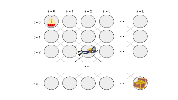
Figure 1: The DeepSea MDP

In Figure 2 we show the time required to ‘solve’ the problem as a function of the depth of the environment, averaged over $5$ seeds for each algorithm. We define ‘time to solve’ to be the first episode at which the agent has reached the rewarding state in at least $10\%$ of the episodes so far. If an agent fails to solve an instance within $10^{5}$ episodes we do not plot that point, which is why some of the traces appear to abruptly stop. We compare two dithering approaches, Q-learning with epsilon-greedy ($\epsilon=0.1$) and soft-Q-learning [18] ($\tau=0.05$), against principled exploration strategies RLSVI [39], UCBVI [7], optimistic Q-learning (OQL) [23], BEB [24], Thompson sampling [38] and two variants of K-learning, one using the $\tau_{t}$ schedule (10) and the other using the optimal choice $\tau_{t}^{\star}$ from solving (11). Soft Q-learning is similar to K-learning with two major differences: the temperature term is a fixed hyperparameter and there is no optimism bonus added to the rewards. These differences prevent soft Q-learning from satisfying a regret bound and typically it cannot solve difficult exploration tasks in general [36]. We also ran comparisons against BOLT [4], UCFH [14], and UCRL2 [21] but they did not perform much better than the dithering approaches and contributed to the clutter in the figure so we do not show them.

As expected, the two ‘dithering’ approaches are unable to handle the problem as the depth exceeds a small value; they fail to solve the problem within $10^{5}$ episodes for problems larger than $L=6$ for epsilon-greedy and $L=14$ for soft-Q-learning. These approaches are taking time exponential in the size of the problem to solve the problem, which is seen by comparing their performance to the grey dashed line which plots $2^{L-1}$. The other approaches scale more gracefully, however clearly Thompson sampling and K-learning are the most efficient. The optimal choice of K-learning appears to perform slightly better than the scheduled temperature variant, which is unsurprising since it is derived from a tighter upper bound on the regret.

In Figures 3 and 4 we show the progress of K-learning using $\tau_{t}^{\star}$ and Soft Q-learning for a single seed running on the $L=50$ depth DeepSea environment. In the top row of each figure we show the value of each state over time, defined for K-learning as

$$\tilde{V}_{l}^{t}(s)=\tau_{t}\log\sum_{a\in\mathcal{A}}\exp(K_{l}^{t}(s,a)/\tau_{t}),$$ (14)

and analogously for Soft Q-learning. The bottom row shows the log of the visitation counts over time. Although both approaches start similarly, they quickly diverge in their behavior. If we examine the K-learning plots, it is clear that the agent is visiting more of the bottom row as the episodes proceed. This is driven by the fact that the value, which incorporates the epistemic uncertainty, is high for the unvisited states. Concretely, take the $t=300$ case; at this point the K-learning agent has not yet visited the rewarding bottom right state, but the value is very high for that region of the state space and shortly after this it reaches the reward for the first time. By the $t=1000$ plot the agent is travelling along the diagonal to gather the reward consistently. Contrast this to Soft Q-learning, where the agent does not make it even halfway across the grid after $t=1000$ episodes. This is because the soft Q-values do not capture any uncertainty about the environment, so the agent has no incentive to explore and visit new states. The only exploration that soft Q-learning is performing is merely the local dithering arising from using a Boltzmann policy with a nonzero temperature. Indeed, the soft value function barely changes in this case since the agent is consistently gathering zero-mean rewards; any fluctuation in the value function arises merely from the noise in the random rewards.

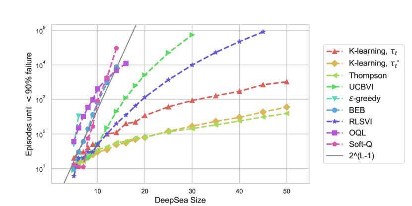
Figure 2: Learning time on DeepSea.

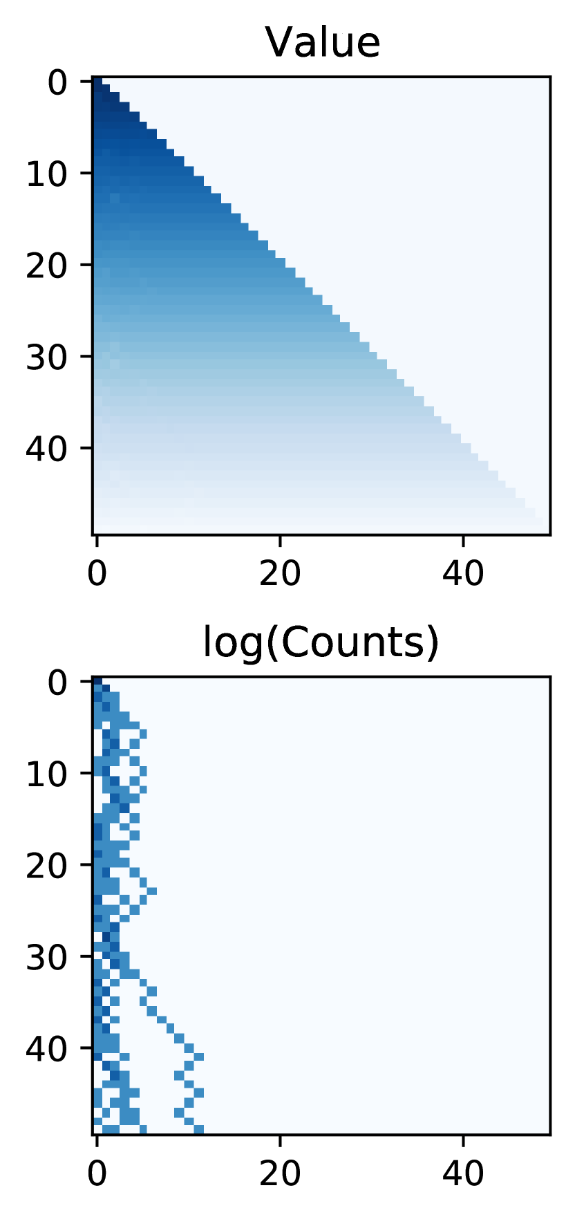
(a) $t=5$.

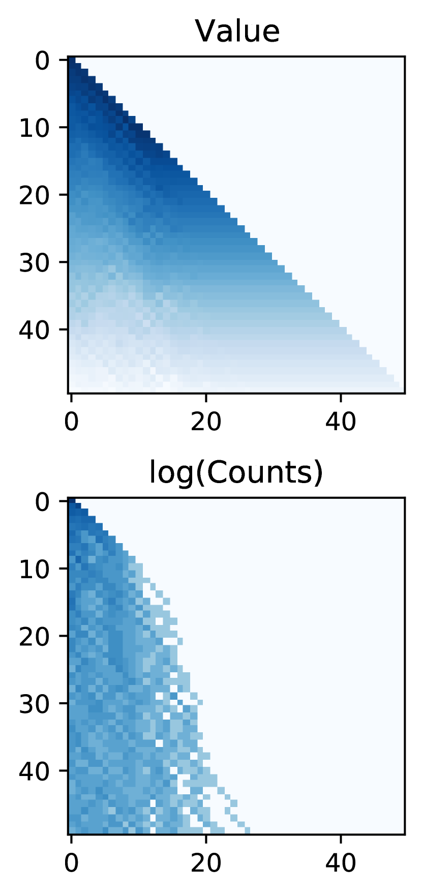
(b) $t=50$.

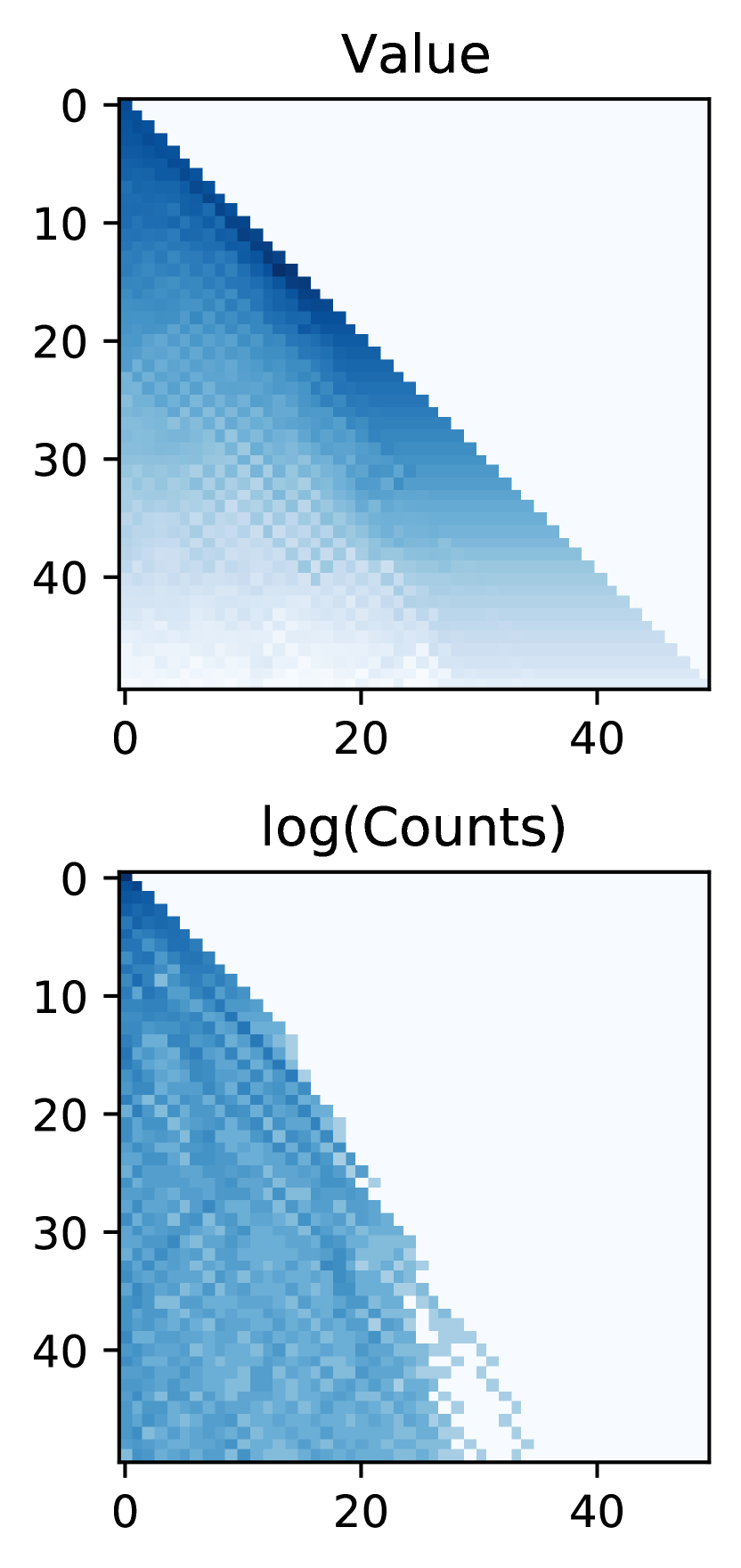
(c) $t=100$.

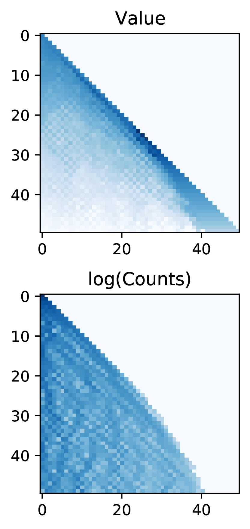
(d) $t=300$.

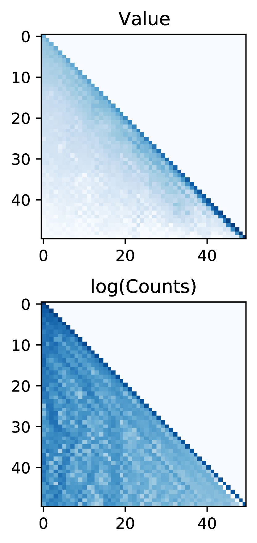
(e) $t=1000$.

Figure 3: Value (as defined in (14)) and log visitation count for each state in DeepSea under K-learning using $\tau_{t}^{\star}$. Darker color indicates larger value.

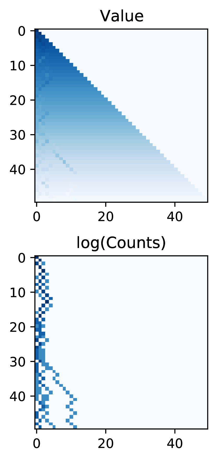
(a) $t=5$.

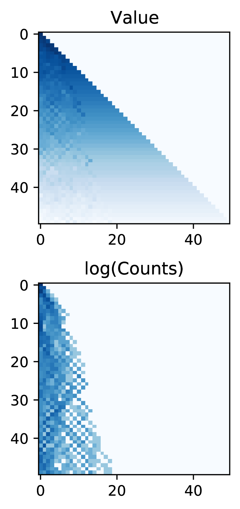
(b) $t=50$.

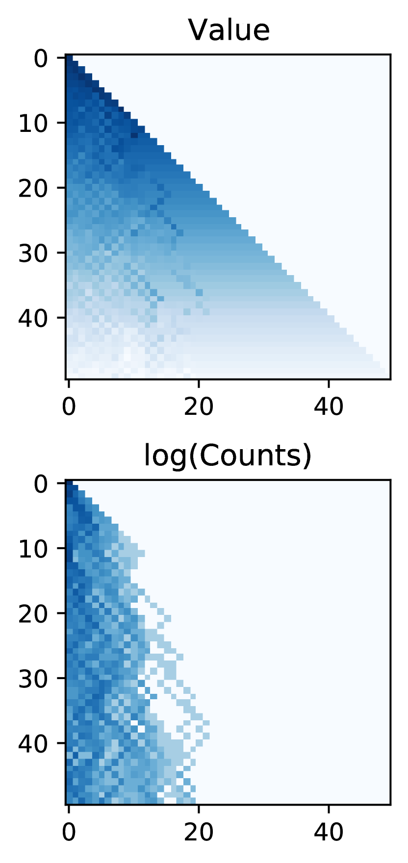
(c) $t=100$.

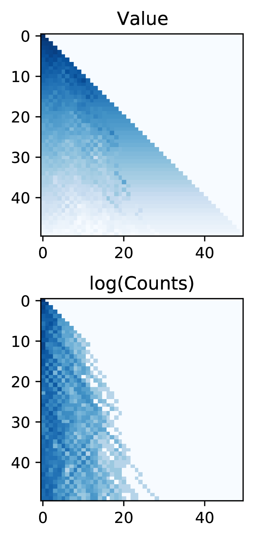
(d) $t=300$.

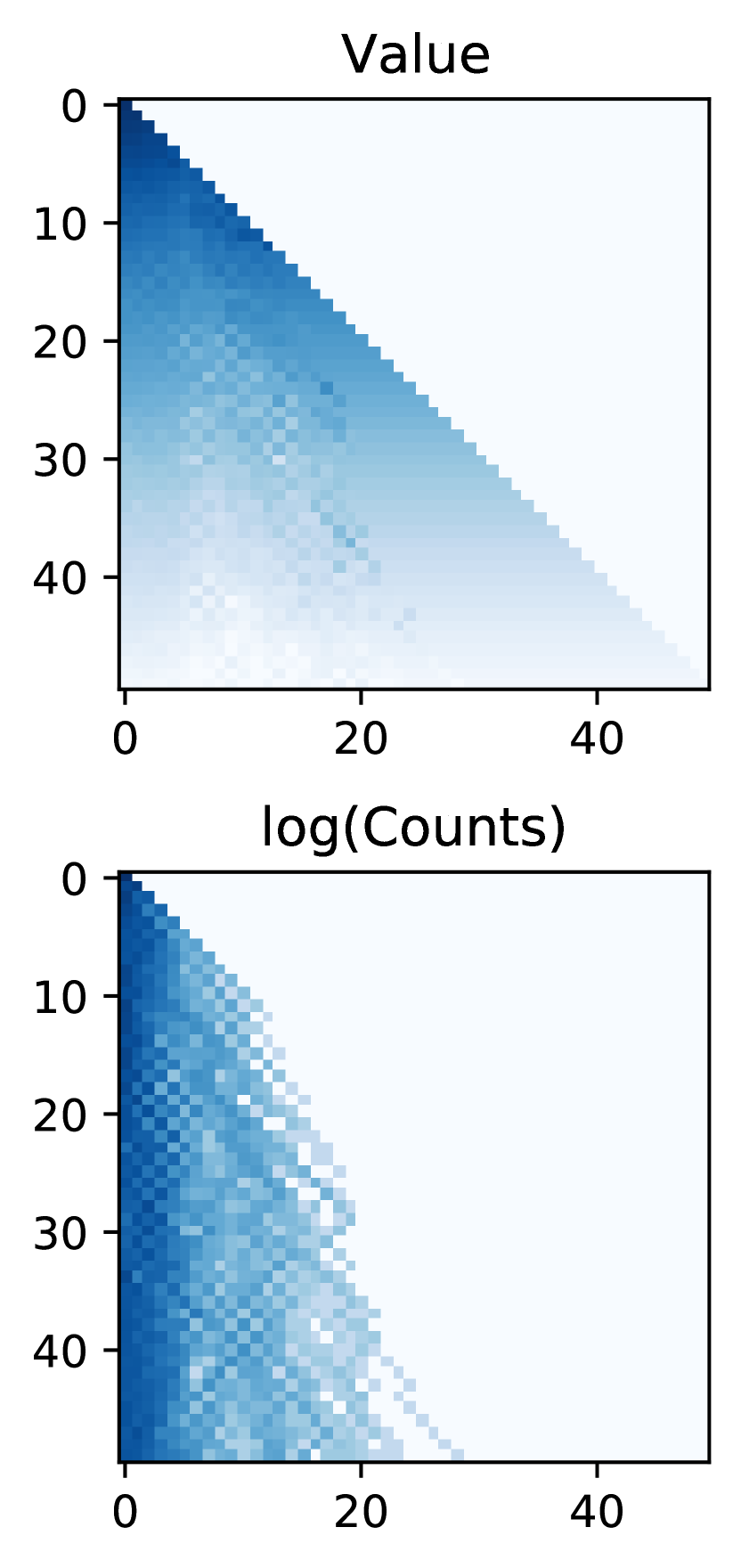
(e) $t=1000$.

Figure 4: Value (as defined in (14)) and log visitation count for each state in DeepSea under soft Q-learning. Darker color indicates larger value.

5 Conclusions

In this work we endowed a reinforcement learning agent with a risk-seeking utility, which encourages the agent to take actions that lead to less epistemically certain states. This yields a Bayesian algorithm with a bound on regret which matches the best-known regret bound for Thompson sampling up to log factors and is close to the known lower bound. We call the algorithm ‘K-learning’, since the ‘K-values’ capture something about the epistemic knowledge that the agent can obtain by visiting each state-action. In the limit of zero uncertainty the K-values reduce to the optimal Q-values.

Although K-learning and Thompson sampling have similar theoretical and empirical performance, K-learning has some advantages. For one, it was recently shown that K-learning extends naturally to the case of two-player games and continues to enjoy a sub-linear regret bound, whereas Thompson sampling can suffer linear regret [34]. Secondly, Thompson sampling requires sampling from the posterior over MDPs and solving the sampled MDP exactly at each episode. This means that Thompson sampling does not have a ‘fixed’ policy at any given episode since it is determined by the posterior information plus a sampling procedure. This is typically a deterministic policy, and it can vary significantly from episode to episode. By contrast K-learning has a single fixed policy at each episode, the Boltzmann distribution over the K-values, and it is determined entirely from the posterior information (i.e., no sampling). Moreover, K-learning requires solving a Bellman equation that changes slowly as more data is accumulated, so the optimal K-values at one episode are close to the optimal K-values for the next episode, and similarly for the policies. This suggests the possibility of approximating K-learning in an online manner and making use of modern deep RL techniques such as representing the K-values using a deep neural network [29]. This is in line with the purpose of this paper, which is not to get the best theoretical regret bound, but instead to derive an algorithm that is close to something that is practical to implement in a real RL setting. Soft-max updates, maximum-entropy RL, and related algorithms are very popular in deep RL. However, they are not typically well motivated and they cannot perform deep-exploration. This paper tackles both those problems since the soft-max update, entropy regularization, and deep-exploration all fall out naturally from a utility maximization point of view. The popularity and success of these other approaches, despite their evident shortcomings in data efficiency, suggest that incorporating changes derived from K-learning could yield big performance improvements in real-world settings. We leave exploring that avenue to future work.

Checklist

1. For all authors…

   1. Do the main claims made in the abstract and introduction accurately reflect the paper’s contributions and scope? [Yes]

   2. Did you describe the limitations of your work? [Yes]

   3. Did you discuss any potential negative societal impacts of your work? [No] This paper is a purely theoretical work with little societal impact.

   4. Have you read the ethics review guidelines and ensured that your paper conforms to them? [Yes]

2. If you are including theoretical results…

   1. Did you state the full set of assumptions of all theoretical results? [Yes]

   2. Did you include complete proofs of all theoretical results? [Yes]

3. If you ran experiments…

   1. Did you include the code, data, and instructions needed to reproduce the main experimental results (either in the supplemental material or as a URL)? [No] We included a description of the data generation process for the simulations we ran.

   2. Did you specify all the training details (e.g., data splits, hyperparameters, how they were chosen)? [N/A] These experiments involved no training on external data.

   3. Did you report error bars (e.g., with respect to the random seed after running experiments multiple times)? [No] I produced Fig 2 with error bars, but it looked very cluttered and obscured the message without providing any additional insight.

   4. Did you include the total amount of compute and the type of resources used (e.g., type of GPUs, internal cluster, or cloud provider)? [Yes] Included in appendix.

4. If you are using existing assets (e.g., code, data, models) or curating/releasing new assets…

   1. If your work uses existing assets, did you cite the creators? [N/A]

   2. Did you mention the license of the assets? [N/A]

   3. Did you include any new assets either in the supplemental material or as a URL? [N/A]

   4. Did you discuss whether and how consent was obtained from people whose data you’re using/curating? [N/A]

   5. Did you discuss whether the data you are using/curating contains personally identifiable information or offensive content? [N/A]

5. If you used crowdsourcing or conducted research with human subjects…

   1. Did you include the full text of instructions given to participants and screenshots, if applicable? [N/A]

   2. Did you describe any potential participant risks, with links to Institutional Review Board (IRB) approvals, if applicable? [N/A]

   3. Did you include the estimated hourly wage paid to participants and the total amount spent on participant compensation? [N/A]

Appendix A Appendix

This appendix is dedicated to proving Theorem 1. First, we introduce some notation. The cumulant generating function of random variable $X:\Omega\rightarrow{\mathbb{R}}$ is given by

$$G^{X}(\beta)=\log\mathbb{E}\exp(\beta X).$$

We shall denote the cumulant generating function of $\mu_{l}(s,a)$ at time $t$ as $G^{\mu|t}_{l}(s,a,\cdot)$ and similarly the cumulant generating function of $Q_{l}^{\star}(s,a)$ at time $t$ as $G_{l}^{Q|t}(s,a,\cdot)$, specifically

$$G^{\mu|t}_{l}(s,a,\beta)=\log\mathbb{E}^{t}\exp(\beta\mu_{l}(s,a)),\quad G^{Q|t}_{l}(s,a,\beta)=\log\mathbb{E}^{t}\exp(\beta Q^{\star}_{l}(s,a)),$$

for $l=1,\ldots,L$.

Theorem 1.

Under assumption 1 the K-learning algorithm 1 satisfies Bayes regret bound

$$\begin{split}\mathcal{BR}_{\phi}(T)&\leq 2\sqrt{(\sigma^{2}+L^{2})SAT\log A(1+\log T/L)}\\ &=\tilde{O}(L\sqrt{SAT}).\end{split}$$ (15)

Proof.

Lemma 1 tells us that $G^{Q|t}(s,a,\beta)$ satisfies a Bellman inequality for any $\beta\geq 0$. This implies that for fixed $\tau_{t}\geq 0$ the certainty equivalent values $\mathcal{Q}^{t}_{l}=\tau_{t}G_{l}^{Q|t}(s,a,1/\tau_{t})$ satisfy a Bellman inequality with optimistic Bellman operator $\mathcal{B}^{t}$ defined in Eq. (6), i.e.,

$$\mathcal{Q}^{t}_{l}\leq\mathcal{B}_{l}^{t}(\tau_{t},\mathcal{Q}^{t}_{l+1}),$$

for $l=1,\ldots,L$, where $\mathcal{Q}^{t}_{L+1}\equiv 0$. By construction the K-values $K^{t}$ are the unique fixed point of the optimistic Bellman operator. That is, $K^{t}$ has $K^{t}_{L+1}\equiv 0$ and

$$K^{t}_{l}=\mathcal{B}^{t}_{l}(\tau_{t},K^{t}_{l+1})$$ (16)

for $l=1,\ldots,L$. Since log-sum-exp is nondecreasing it implies that the operator $\mathcal{B}^{t}_{l}(\tau,\cdot)$ is nondecreasing for any $\tau\geq 0$, i.e., if $x\geq y$ pointwise then $\mathcal{B}^{t}_{l}(\tau,x)\geq\mathcal{B}^{t}_{l}(\tau,y)$ pointwise for each $l$. Now assume that for some $l$ we have $K^{t}_{l+1}\geq\mathcal{Q}^{t}_{l+1}$, then

$$K^{t}_{l}=\mathcal{B}^{t}_{l}(\tau_{t},K^{t}_{l+1})\geq\mathcal{B}^{t}_{l}(\tau_{t},\mathcal{Q}^{t}_{l+1})\geq\mathcal{Q}^{t}_{l},$$

and the base case holds since $K^{t}_{L+1}=\mathcal{Q}^{t}_{L+1}\equiv 0$. This fact, combined with Lemma 4 implies that

$$\mathbb{E}^{t}\max_{a}Q_{l}^{\star}(s,a)\leq\tau_{t}\log\sum_{a\in\mathcal{A}}\exp(\mathcal{Q}^{t}_{l}(s,a)/\tau_{t})\leq\tau_{t}\log\sum_{a\in\mathcal{A}}\exp(K_{l}^{t}(s,a)/\tau_{t})$$ (17)

since log-sum-exp is increasing and $\tau_{t}\geq 0$. The following variational identity yields the policy that the agent will follow:

$$\tau_{t}\log\sum_{a\in\mathcal{A}}\exp(K_{l}^{t}(s,a)/\tau_{t})=\max_{\pi_{l}(s,\cdot)\in\Delta_{A}}\left(\sum_{a\in\mathcal{A}}\pi_{l}(s,a)K_{l}^{t}(s,a)+\tau_{t}H(\pi_{l}(s,\cdot))\right)$$

for any state $s$, where $\Delta_{A}$ is the probability simplex of dimension $A-1$ and $H$ denotes the entropy, i.e., $H(\pi(s,\cdot))=-\sum_{a\in\mathcal{A}}\pi(s,a)\log\pi(s,a)$ [13]. The maximum is achieved by the policy

$$\pi^{t}_{l}(s,a)\propto\exp(K_{l}^{t}(s,a)/\tau_{t}).$$

This comes from taking the Legendre transform of negative entropy term (equivalently, log-sum-exp and negative entropy are convex conjugates [10, Example 3.25]). The fact that (9) achieves the maximum is readily verified by substitution.

Now we consider the Bayes regret of an agent following policy (9), starting from (4) we have

$$\begin{split}\mathcal{BR}_{\phi}(T)&\overset{\scriptscriptstyle(a)}{=}\mathbb{E}\sum_{t=1}^{N}\mathbb{E}_{s\sim\rho}\mathbb{E}^{t}(V_{1}^{\star}(s)-V_{1}^{\pi^{t}}(s))\\ &=\mathbb{E}\sum_{t=1}^{N}\mathbb{E}_{s\sim\rho}\mathbb{E}^{t}\Big{(}\max_{a}Q_{1}^{\star}(s,a)-\sum_{a\in\mathcal{A}}\pi_{1}^{t}(s,a)Q_{1}^{\pi^{t}}(s,a)\Big{)}\\ &\overset{\scriptscriptstyle(b)}{\leq}\mathbb{E}\sum_{t=1}^{N}\mathbb{E}_{s\sim\rho}\Big{(}\tau_{t}\log\sum_{a\in\mathcal{A}}\exp(K_{1}^{t}(s,a)/\tau_{t})-\sum_{a\in\mathcal{A}}\pi_{1}^{t}(s,a)\mathbb{E}^{t}Q_{1}^{\pi^{t}}(s,a)\Big{)}\\ &\overset{\scriptscriptstyle(c)}{\leq}\mathbb{E}\sum_{t=1}^{N}\mathbb{E}_{s\sim\rho}\bigg{(}\sum_{a\in\mathcal{A}}\pi_{1}^{t}(s,a)\Big{(}K_{1}^{t}(s,a)-\mathbb{E}^{t}Q_{1}^{\pi^{t}}(s,a)\Big{)}+\tau_{t}H(\pi_{1}^{t}(s))\bigg{)}\end{split}$$ (18)

where (a) follows from the tower property of conditional expectation where the outer expectation is with respect to $\mathcal{F}_{1},\mathcal{F}_{2},\ldots$, (b) is due to (17) and the fact that $\pi^{t}$ is $\mathcal{F}_{t}$-measurable, and (c) is due to the fact that the policy the agent is following is the policy (9). If we denote by

$$\Delta_{l}^{t}(s)=\sum_{a\in\mathcal{A}}\pi_{l}^{t}(s,a)\left(K_{l}^{t}(s,a)-\mathbb{E}^{t}Q_{l}^{\pi^{t}}(s,a)\right)+\tau_{t}H(\pi_{l}^{t}(s))$$

then we can write the previous bound simply as

$$\mathcal{BR}_{\phi}(T)\leq\mathbb{E}\sum_{t=1}^{N}\mathbb{E}_{s\sim\rho}\Delta_{1}^{t}(s).$$

We can interpret $\Delta^{t}_{l}(s)$ as a bound on the expected regret in that episode when started at state $s$. Let us denote

$$\tilde{G}_{l}^{\mu|t}(s,a,\beta)=G_{l}^{\mu|t}(s,a,\beta)+\frac{(L-l)^{2}\beta^{2}}{2(n_{l}^{t}(s,a)\vee 1)}.$$

Now we shall show that for a fixed $\pi^{t}$ and $\tau_{t}\geq 0$ the quantity $\Delta^{t}$ satisfies the following Bellman recursion:

$$\Delta_{l}^{t}(s)=\tau_{t}H(\pi_{l}^{t}(s))+\sum_{a\in\mathcal{A}}\pi_{l}^{t}(s,a)\left(\delta_{l}^{t}(s,a,\tau_{t})+\sum_{s^{\prime}\in\mathcal{S}_{l+1}}\mathbb{E}^{t}(P_{l}(s^{\prime}\mid s,a))\Delta_{l+1}^{t}(s^{\prime})\right)$$ (19)

for $s\in\mathcal{S}$, $l=1,\ldots,L$, and $\Delta^{t}_{L+1}\equiv 0$, where

$$\delta_{l}^{t}(s,a,\tau)=\tau\tilde{G}_{l}^{\mu|t}(s,a,1/\tau)-\mathbb{E}^{t}\mu_{l}(s,a)\leq\frac{\sigma^{2}+(L-l)^{2}}{2\tau(n_{l}^{t}(s,a)\vee 1)},$$ (20)

where the inequality follows from assumption 1 which allows us to bound $G_{l}^{\mu|t}$ as

$$\tau G_{l}^{\mu|t}(s,a,1/\tau)\leq\mathbb{E}^{t}\mu_{l}(s,a)+\frac{\sigma^{2}}{2\tau(n_{l}^{t}(s,a)\vee 1)}$$

for all $\tau\geq 0$. We have that

$$\begin{split}\mathbb{E}^{t}Q_{l}^{\pi^{t}}(s,a)&\overset{\scriptscriptstyle(a)}{=}\mathbb{E}^{t}\Big{(}\mu_{l}(s,a)+\sum_{s^{\prime}\in\mathcal{S}_{l+1}}P_{l}(s^{\prime}\mid s,a)V_{l+1}^{\pi^{t}}(s^{\prime})\Big{)}\\ &\overset{\scriptscriptstyle(b)}{=}\mathbb{E}^{t}\mu_{l}(s,a)+\sum_{s^{\prime}\in\mathcal{S}_{l+1}}\mathbb{E}^{t}P_{l}(s^{\prime}\mid s,a)\mathbb{E}^{t}V_{l+1}^{\pi^{t}}(s^{\prime})\\ &\overset{\scriptscriptstyle(c)}{=}\mathbb{E}^{t}\mu_{l}(s,a)+\sum_{s^{\prime}\in\mathcal{S}_{l+1}}\mathbb{E}^{t}P_{l}(s^{\prime}\mid s,a)\sum_{a^{\prime}\in\mathcal{A}}\pi_{l+1}^{t}(s^{\prime},a^{\prime})\mathbb{E}^{t}Q_{l+1}^{\pi^{t}}(s^{\prime},a^{\prime}),\end{split}$$ (21)

where (a) is the Bellman Eq. (2), (b) holds due to the fact that the transition function and the value function at the next state are conditionally independent, (c) holds since $\pi^{t}$ is $\mathcal{F}_{t}$ measurable.

Now we expand the definition of $\Delta^{t}$, using the Bellman equation that the K-values satisfy and Eq. (21) for the Q-values

$$\Delta_{l}^{t}(s) =\tau_{t}H(\pi_{l}^{t}(s))+\sum_{a\in\mathcal{A}}\pi_{l}^{t}(s,a)\Big{(}\tau_{t}\tilde{G}_{l}^{\mu|t}(s,a,1/\tau_{t})-\mathbb{E}^{t}\mu_{l}(s,a)+$$

$$\qquad\sum_{s^{\prime}\in\mathcal{S}_{l+1}}\mathbb{E}^{t}P_{l}(s^{\prime}\mid s,a)\big{(}\tau_{t}\log\sum_{a^{\prime}\in\mathcal{A}}\exp K_{l+1}^{t}(s^{\prime},a^{\prime})/\tau_{t}-\sum_{a^{\prime}\in\mathcal{A}}\pi_{l+1}^{t}(s^{\prime},a^{\prime})\mathbb{E}^{t}Q_{l+1}^{\pi^{t}}(s^{\prime},a^{\prime})\big{)}\Big{)}$$

$$=\tau_{t}H(\pi_{l}^{t}(s))+\sum_{a\in\mathcal{A}}\pi_{l}^{t}(s,a)\bigg{(}\delta_{l}^{t}(s,a,\tau_{t})+$$

$$\qquad\sum_{s^{\prime}\in\mathcal{S}_{l+1}}\mathbb{E}^{t}P_{l}(s^{\prime}\mid s,a)\Big{(}\tau_{t}H(\pi_{l+1}^{t}(s^{\prime}))+\sum_{a^{\prime}\in\mathcal{A}}\pi_{l+1}^{t}(s^{\prime},a^{\prime})\Big{(}K_{l+1}^{t}(s^{\prime},a^{\prime})-\mathbb{E}^{t}Q_{l+1}^{\pi^{t}}(s^{\prime},a^{\prime})\Big{)}\Big{)}\bigg{)}$$

$$=\tau_{t}H(\pi_{l}^{t}(s))+\sum_{a\in\mathcal{A}}\pi_{l}^{t}(s,a)\bigg{(}\delta_{l}^{t}(s,a,\tau_{t})+\sum_{s^{\prime}\in\mathcal{S}_{l+1}}\mathbb{E}^{t}P_{l}(s^{\prime}\mid s,a)\Delta_{l+1}^{t}(s^{\prime})\bigg{)},$$

where we used the variational representation (8). We shall use this to ‘unroll’ $\Delta^{t}$ along the MDP, allowing us to write the regret upper bound using only local quantities.

An occupancy measure is the probability that the agent finds itself in state $s$ and takes action $a$. Let $\lambda_{l}^{t}(s,a)$ be the expected occupancy measure for state $s$ and action $a$ under the policy $\pi^{t}$ at time $t$, that is $\lambda_{1}^{t}(s,a)=\pi_{1}^{t}(s,a)\rho(s)$, and then it satisfies the forward recursion

$$\lambda_{l+1}^{t}(s^{\prime},a^{\prime})=\pi_{l}^{t}(s^{\prime},a^{\prime})\sum_{(s,a)\in\mathcal{S}_{l}\times\mathcal{A}}\mathbb{E}^{t}(P_{l}(s^{\prime}\mid s,a))\lambda_{l}^{t}(s,a),$$

for $l=1,\ldots,L$, and note that $\sum_{(s,a)\in\mathcal{S}_{l}\times\mathcal{A}}\lambda_{l}^{t}(s,a)=1$ and so it is a valid probability distribution over $\mathcal{S}_{l}\times\mathcal{A}$ for each $l$. Now let us define the following function

$$\Phi^{t}(\tau,\lambda)=\sum_{l=1}^{L}\sum_{(s,a)\in\mathcal{S}_{l}\times\mathcal{A}}\lambda^{t}_{l}(s,a)\left(\tau H\left(\frac{\lambda_{l}^{t}(s)}{\sum_{b}\lambda_{l}^{t}(s,b)}\right)+\delta_{l}^{t}(s,a,\tau)\right).$$ (22)

where $\lambda^{t}(s)$ is the vector corresponding to the occupancy measure values at state $s$. One can see that by unrolling the definition of $\Delta^{t}$ in (19) we have that

$$\mathbb{E}_{s\sim\rho}\Delta_{1}^{t}(s)=\Phi^{t}(\tau_{t},\lambda^{t}).$$

In order to prove the Bayes regret bound, we must bound this $\Phi^{t}$ function. For the case of $\tau_{t}$ annealed according to the schedule of (10) and the associated expected occupancy measure $\lambda^{t}$ we do this using lemma 3. For the case of $\tau^{\star}_{t}$ the solution to (11) and the associated expected occupancy measure $\lambda^{t\star}$ lemma 5 proves that

$$\Phi^{t}(\tau^{\star}_{t},\lambda^{t\star})\leq\Phi^{t}(\tau_{t},\lambda^{t}),$$

and so it satisfies the same regret bound as the annealed parameter. This result concludes the proof. ∎

A.1 Proof of Bellman inequality lemma 1

Lemma 1.

The cumulant generating function of the posterior for the optimal Q-values satisfies the following Bellman inequality for all $\beta\geq 0$, $l=1,\ldots,L$:

$$G_{l}^{Q|t}(s,a,\beta)\leq\tilde{G}_{l}^{\mu|t}(s,a,\beta)+\sum_{s^{\prime}\in\mathcal{S}_{l+1}}\mathbb{E}^{t}P_{l}(s^{\prime}\mid s,a)\log\sum_{a^{\prime}\in\mathcal{A}}\exp G_{l+1}^{Q|t}(s^{\prime},a^{\prime},\beta).$$

where

$$\tilde{G}_{l}^{\mu|t}(s,a,\beta)=G_{l}^{\mu|t}(s,a,\beta)+\frac{(L-l)^{2}\beta^{2}}{2(n_{l}^{t}(s,a)\vee 1)}.$$

Proof.

We begin by applying the definition of the cumulant generating function

$$\begin{split}G_{l}^{Q|t}(s,a,\beta)&=\log\mathbb{E}^{t}\exp\beta Q_{l}^{\star}(s,a)\\ &=\log\mathbb{E}^{t}\exp\Big{(}\beta\mu_{l}(s,a)+\beta\sum_{s^{\prime}\in\mathcal{S}_{l+1}}P_{l}(s^{\prime}\mid s,a)V_{l+1}^{\star}(s^{\prime})\Big{)}\\ &=G_{l}^{\mu|t}(s,a,\beta)+\log\mathbb{E}^{t}\exp\Big{(}\beta\sum_{s^{\prime}\in\mathcal{S}_{l+1}}P_{l}(s^{\prime}\mid s,a)V_{l+1}^{\star}(s^{\prime})\Big{)}\end{split}$$ (23)

where $G_{l}^{\mu|t}$ is the cumulant generating function for $\mu$, and where the first equality is the Bellman equation for $Q^{\star}$, and the second one follows the fact that $\mu_{l}(s,a)$ is conditionally independent of downstream quantities. Now we must deal with the second term in the above expression.

Assumption 1 says that the prior over the transition function $P_{l}(~{}\cdot\mid s,a)$ is Dirichlet, so let us denote the parameter of the Dirichlet distribution $\alpha_{l}^{0}(s,a)\in{\mathbb{R}}_{+}^{S}$ for each $(s,a)$, and we make the additional mild assumption that $\sum_{s^{\prime}\in\mathcal{S}_{l+1}}\alpha_{l}^{0}(s,a,s^{\prime})\geq 1$, i.e., we start with a total pseudo-count of at least one for every state-action. Since the likelihood for the transition function is a Categorical distribution, conjugacy of the categorical and Dirichlet distributions implies that the posterior over $P_{l}(~{}\cdot\mid s,a)$ at time $t$ is Dirichlet with parameter $\alpha_{l}^{t}(s,a)$, where

$$\alpha_{l}^{t}(s,a,s^{\prime})=\alpha_{l}^{0}(s,a,s^{\prime})+n^{t}_{l}(s,a,s^{\prime})$$

for each $s^{\prime}\in\mathcal{S}_{l+1}$, where $n_{l}^{t}(s,a,s^{\prime})\in{\mathbb{N}}$ is the number of times the agent has been in state $s$, taken action $a$, and transitioned to state $s^{\prime}$ at timestep $l$, and note that $\sum_{s^{\prime}\in\mathcal{S}_{l+1}}n_{l}^{t}(s,a,s^{\prime})=n_{l}^{t}(s,a)$, the total visit count to $(s,a)$.

Our analysis will make use of the following definition and associated lemma from [40]. Let $X$ and $Y$ be random variables, we say that $X$ is stochastically optimistic for $Y$, written $X\geq_{SO}Y$, if $\mathbb{E}u(X)\geq\mathbb{E}u(Y)$ for any convex increasing function $u$. Stochastic optimism is closely related to the more familiar concept of second-order stochastic dominance, in that $X$ is stochastically optimistic for $Y$ if and only if $-Y$ second-order stochastically dominates $-X$ [19]. We use this definition in the next lemma.

Lemma 2.

Let $Y$ = $\sum_{i=1}^{n}A_{i}b_{i}$ for fixed $b\in{\mathbb{R}}^{n}$ and random variable $A$, where $A$ is Dirichlet with parameter $\alpha\in{\mathbb{R}}^{n}$, and let $X\sim\mathcal{N}(\mu_{X},\sigma_{X}^{2})$ with $\mu_{X}\geq\frac{\sum_{i}\alpha_{i}b_{i}}{\sum_{i}\alpha_{i}}$ and $\sigma_{X}^{2}\geq(\sum_{i}\alpha_{i})^{-1}\mathrm{Span}(b)^{2}$, where $\mathrm{Span(b)}=\max_{i}b_{i}-\min_{j}b_{j}$, then $X\geq_{SO}Y$.

For the proof see [40]. In our case, in the notation of the lemma 2, $A$ will represent the transition function probabilities, and $b$ will represent the optimal values of the next state, i.e., for a given $(s,a)\in\mathcal{S}\times\mathcal{A}$ let $X_{t}$ be a random variable distributed $\mathcal{N}(\mu_{X_{t}},\sigma_{X_{t}}^{2})$ where

$$\mu_{X_{t}}=\sum_{s^{\prime}\in\mathcal{S}_{l+1}}\Big{(}\alpha_{l}^{t}(s,a,s^{\prime})V_{l+1}^{\star}(s^{\prime})/\sum_{x}\alpha_{l}^{t}(s,a,x)\Big{)}=\sum_{s^{\prime}\in\mathcal{S}_{l+1}}\mathbb{E}^{t}(P_{l}(s^{\prime}\mid s,a))V_{l+1}^{\star}(s^{\prime})$$

due to the Dirichlet assumption 1. Due to assumption 1 we know that $\mathrm{Span}(V_{l}^{\star}(s))\leq L-l$, so we choose $\sigma_{X_{t}}^{2}=(L-l)^{2}/(n_{l}^{t}(s,a)\vee 1)$. Let $\mathcal{F}^{V}_{t}=\mathcal{F}_{t}\cup\sigma(V^{\star})$ denote the union of $\mathcal{F}_{t}$ and the sigma-algebra generated by $V^{\star}$. Applying lemma 2 and the tower property of conditional expectation we have that for $\beta\geq 0$

$$\begin{split}\mathbb{E}^{t}\exp\Big{(}\beta\sum_{s^{\prime}\in\mathcal{S}_{l+1}}P_{l}(s^{\prime}\mid s,a)V_{l+1}^{\star}(s^{\prime})\Big{)}&=\mathbb{E}_{V_{l+1}^{\star}}\bigg{(}\mathbb{E}_{P}\Big{(}\exp\beta\Big{(}\sum_{s^{\prime}\in\mathcal{S}_{l+1}}P_{l}(s^{\prime}\mid s,a)V_{l+1}^{\star}(s^{\prime})\Big{)}\big{|}\mathcal{F}^{V}_{t}\Big{)}\Big{|}\mathcal{F}_{t}\bigg{)}\\ &\leq\mathbb{E}_{V_{l+1}^{\star}}\left(\mathbb{E}_{X_{t}}(\exp\beta X_{t}|\mathcal{F}^{V}_{t})\Big{|}\mathcal{F}_{t}\right)\\ &=\mathbb{E}_{V_{l+1}^{\star}}\left(\exp(\mu_{X_{t}}\beta+\sigma_{X_{t}}^{2}\beta^{2}/2)\Big{|}\mathcal{F}_{t}\right)\\ &=\mathbb{E}_{V_{l+1}^{\star}}^{t}\exp\Big{(}\beta\sum_{s^{\prime}\in\mathcal{S}_{l+1}}\mathbb{E}^{t}P_{l}(s^{\prime}\mid s,a)V_{l+1}^{\star}(s^{\prime})+\sigma_{X_{t}}^{2}\beta^{2}/2\Big{)},\end{split}$$ (24)

the first equality is the tower property of conditional expectation, the inequality comes from the fact that $P_{l}(s^{\prime}\mid s,a)$ is conditionally independent of $V_{l+1}^{\star}(s^{\prime})$ and applying lemma 2, the next equality is applying the moment generating function for the Gaussian distribution and the final equality is substituting in for $\mu_{X_{t}}$. Now applying this result to the last term in (23)

$$\log\mathbb{E}^{t}\exp\Big{(}\beta\sum_{s^{\prime}\in\mathcal{S}_{l+1}}P_{l}(s^{\prime}\mid s,a)V_{l+1}^{\star}(s^{\prime})\Big{)}$$

$$\qquad\overset{\scriptscriptstyle(a)}{\leq}\log\mathbb{E}^{t}_{V_{l+1}^{\star}}\exp\Big{(}\beta\sum_{s^{\prime}\in\mathcal{S}_{l+1}}\mathbb{E}^{t}P_{l}(s^{\prime}\mid s,a)V_{l+1}^{\star}(s^{\prime})+\sigma_{X_{t}}^{2}\beta^{2}/2\Big{)}$$

$$\qquad\overset{\scriptscriptstyle(b)}{=}\log\mathbb{E}^{t}_{Q_{l+1}^{\star}}\exp\Big{(}\beta\sum_{s^{\prime}\in\mathcal{S}_{l+1}}\mathbb{E}^{t}P_{l}(s^{\prime}\mid s,a)\max_{a^{\prime}}Q_{l+1}^{\star}(s^{\prime},a^{\prime})\Big{)}+\sigma_{X_{t}}^{2}\beta^{2}/2$$

$$\qquad\overset{\scriptscriptstyle(c)}{\leq}\sum_{s^{\prime}\in\mathcal{S}_{l+1}}\mathbb{E}^{t}P_{l}(s^{\prime}\mid s,a)\log\mathbb{E}^{t}_{Q_{l+1}^{\star}}\exp\Big{(}\beta\max_{a^{\prime}}Q_{l+1}^{\star}(s^{\prime},a^{\prime})\Big{)}+\sigma_{X_{t}}^{2}\beta^{2}/2$$

$$\qquad\overset{\scriptscriptstyle(d)}{\leq}\sum_{s^{\prime}\in\mathcal{S}_{l+1}}\mathbb{E}^{t}P_{l}(s^{\prime}\mid s,a)\log\sum_{a^{\prime}\in\mathcal{A}}\exp G_{l+1}^{Q|t}(s^{\prime},a^{\prime})(\beta)+\frac{\beta^{2}(L-l)^{2}}{2(n_{l}^{t}(s,a)\vee 1)}$$

where (a) follows from Eq. (24)) and the fact that log is increasing, (b) is replacing $V^{\star}$ with $Q^{\star}$, (c) uses Jensen’s inequality and the fact that $\log\mathbb{E}\exp(\cdot)$ is convex, and (d) follows by substituting in for $\sigma_{X_{t}}$ and since the max of a collection of positive numbers is less than the sum. Combining this and (23) the inequality immediately follows. ∎

A.2 Proof of lemma 3

Lemma 3.

Following the policy induced by expected occupancy measure $\lambda_{l}^{t}\in[0,1]^{|\mathcal{S}_{l}|\times A}$, $l=1,\ldots,L$, and the temperature schedule $\tau_{t}$ in (10) we have

$$\mathbb{E}\sum_{t=1}^{N}\Phi^{t}(\tau_{t},\lambda^{t})\leq 2\sqrt{(\sigma^{2}+L^{2})SAT\log A(1+\log T/L)}.$$

Proof.

Starting from the definition of $\Phi$

$$\Phi^{t}(\tau_{t},\lambda^{t}) =\sum_{l=1}^{L}\sum_{(s,a)\in\mathcal{S}_{l}\times\mathcal{A}}\lambda_{l}^{t}(s,a)\left(\tau_{t}H\left(\frac{\lambda_{l}^{t}(s)}{\sum_{b}\lambda_{l}^{t}(s,b)}\right)+\delta^{t}(s,a,\tau_{t})\right)$$

$$\leq\tau_{t}L\log A+\tau^{-1}_{t}\sum_{l=1}^{L}\sum_{(s,a)\in\mathcal{S}_{l}\times\mathcal{A}}\lambda^{t}(s,a)\frac{(\sigma^{2}+L^{2})}{2(n_{l}^{t}(s,a)\vee 1)}$$

which comes from the sub-Gaussian assumption on $G_{l}^{\mu|t}$ and the fact that entropy satisfies $H(\pi(\lambda_{s}))\leq\log A$ for all $s$. These two terms summed up to $N$ determine our regret bound, and we shall bound each one independently. To bound the first term:

$$L\log A\sum_{t=1}^{N}\tau_{t} \leq(1/2)\sqrt{(\sigma^{2}+L^{2})LSA\log A(1+\log T/L)}\sum_{t=1}^{N}1/\sqrt{t}$$

$$\leq\sqrt{(\sigma^{2}+L^{2})SAT\log A(1+\log T/L)},$$

since $\sum_{t=1}^{N}1/\sqrt{t}\leq\int_{t=0}^{N}1/\sqrt{t}=2\sqrt{N}$, and recall that $N=\lceil T/L\rceil$. For simplicity we shall take $T=NL$, i.e., we are measuring regret at episode boundaries; this only changes whether or not there is a small fractional episode term in the regret bound or not.

To bound the second term we shall use the pigeonhole principle lemma 6, which requires knowledge of the process that generates the counts at each timestep, which is access to the true occupancy measure in our case. The quantity $\lambda^{t}$ is not the true occupancy measure at time $t$, which we shall denote by $\nu^{t}$, since that depends on $P$ which we don’t have access to (we only have a posterior distribution over it). However it is the expected occupancy measure conditioned on $\mathcal{F}_{t}$, i.e., $\lambda^{t}=\mathbb{E}^{t}\nu^{t}$, which is easily seen by starting from $\lambda_{1}^{t}(s,a)=\pi_{1}^{t}(s,a)\rho(s)=\nu_{1}^{t}(s,a)$, and then inductively using:

$$\mathbb{E}^{t}\nu_{l+1}^{t}(s^{\prime},a^{\prime}) =\mathbb{E}^{t}\Big{(}\pi_{l+1}^{t}(s^{\prime},a^{\prime})\sum_{(s,a)\in\mathcal{S}_{l}\times\mathcal{A}}P_{l}(s^{\prime}\mid s,a)\nu_{l}^{t}(s,a)\Big{)}$$

$$=\pi_{l+1}^{t}(s^{\prime},a^{\prime})\sum_{(s,a)\in\mathcal{S}_{l}\times\mathcal{A}}\mathbb{E}^{t}(P_{l}(s^{\prime}\mid s,a))\mathbb{E}^{t}\nu_{l}^{t}(s,a)$$

$$=\pi_{l+1}^{t}(s^{\prime},a^{\prime})\sum_{(s,a)\in\mathcal{S}_{l}\times\mathcal{A}}\mathbb{E}^{t}(P_{l}(s^{\prime}\mid s,a))\lambda_{l}^{t}(s,a)$$

$$=\lambda_{l+1}^{t}(s^{\prime},a^{\prime})$$

for $l=1,\ldots,L$, where we used the fact that $\pi^{t}$ is $\mathcal{F}_{t}$-measurable and the fact that $\nu_{l}(s,a)$ is independent of downstream quantities. Now applying lemma 6

$$\mathbb{E}\sum_{t=1}^{N}\sum_{(s,a)\in\mathcal{S}_{l}\times\mathcal{A}}\frac{\lambda^{t}_{l}(s,a)}{n_{l}^{t}(s,a)+1} =\mathbb{E}\sum_{t=1}^{N}\mathbb{E}^{t}\left(\sum_{(s,a)\in\mathcal{S}_{l}\times\mathcal{A}}\frac{\lambda^{t}_{l}(s,a)}{n_{l}^{t}(s,a)+1}\right)$$

$$=\mathbb{E}\left(\sum_{t=1}^{N}\sum_{(s,a)\in\mathcal{S}_{l}\times\mathcal{A}}\frac{\nu^{t}_{l}(s,a)}{n_{l}^{t}(s,a)+1}\right)$$

$$\leq A|\mathcal{S}_{l}|(1+\log N),$$

which follows from the tower property of conditional expectation and since the counts at time $t$ are $\mathcal{F}_{t}$-measurable. From Eq. (10) we know that sequence $\tau^{-1}_{t}$ is increasing, so we can bound the second term as

$$\mathbb{E}\sum_{t=1}^{N}\tau^{-1}_{t}\sum_{l=1}^{L}\sum_{(s,a)\in\mathcal{S}_{l}\times\mathcal{A}}\frac{\lambda_{l}^{t}(s,a)(\sigma^{2}+L^{2})}{2(n_{l}^{t}(s,a)+1)} \leq(1/2)(\sigma^{2}+L^{2})\tau^{-1}_{N}\mathbb{E}\sum_{l=1}^{L}\left(\sum_{t=1}^{N}\sum_{(s,a)\in\mathcal{S}_{l}\times\mathcal{A}}\frac{\lambda_{l}^{t}(s,a)}{n_{l}^{t}(s,a)+1}\right)$$

$$\leq(1/2)(\sigma^{2}+L^{2})\tau^{-1}_{N}\sum_{l=1}^{L}A|\mathcal{S}_{l}|(1+\log N)$$

$$=(1/2)(\sigma^{2}+L^{2})\tau^{-1}_{N}SA(1+\log N)$$

$$=\sqrt{(\sigma^{2}+L^{2})SAT\log A(1+\log T/L)},$$

since $\sum_{l=1}^{L}|\mathcal{S}_{l}|=|\mathcal{S}|=S$ and using $N=\lceil T/L\rceil$. Combining these two bounds we get our result. ∎

A.3 Proof of maximal inequality lemma 4

Lemma 4.

Let $X_{i}:\Omega\rightarrow{\mathbb{R}}$, $i=1,\ldots,n$ be random variables with cumulant generating functions $G^{X_{i}}:{\mathbb{R}}\rightarrow{\mathbb{R}}$, then for any $\tau\geq 0$

$$\mathbb{E}\max_{i}X_{i}\leq\tau\log\sum_{i=1}^{n}\exp G^{X_{i}}(1/\tau).$$ (25)

Proof.

Using Jensen’s inequality

$$\begin{split}\mathbb{E}\max_{i}X_{i}&=\tau\log\exp(\mathbb{E}\max_{i}X_{i}/\tau)\\ &\leq\tau\log\mathbb{E}\max_{i}(\exp X_{i}/\tau)\\ &\leq\tau\log\sum_{i=1}^{n}\mathbb{E}\exp X_{i}/\tau\\ &=\tau\log\sum_{i=1}^{n}\exp G^{X_{i}}(1/\tau),\end{split}$$ (26)

where the inequality comes from the fact that the max over a collection of nonnegative values is less than the sum. ∎

A.4 Derivation of dual to problem (11)

Here we shall the derive the dual problem to the convex optimization problem (11), which will be necessary to prove a regret bound for the case where we choose $\tau^{\star}_{t}$ as the temperature parameter. Recall that the primal problem is

minimize $$\quad\mathbb{E}_{s\sim\rho}(\tau\log\sum_{a\in\mathcal{A}}\exp(K_{1}(s,a)/\tau))$$

subject to $$\quad K_{l}\geq\mathcal{B}^{t}_{l}(\tau,K_{l+1}),\quad l=1,\ldots,L,$$

$$\quad K_{L+1}\equiv 0,$$

in variables $\tau\geq 0$ and $K\in{\mathbb{R}}^{S\times A}$. We shall repeatedly use the variational representation of log-sum-exp terms as in Eq. (8). We introduce dual variable $\lambda\geq 0$ for each of the $L$ Bellman inequality constraints which yields Lagrangian

$$\sum_{s\in\mathcal{S}_{1}}\rho(s)\sum_{a\in\mathcal{A}}(\pi_{1}(s,a)K_{1}(s,a)+\tau H(\pi_{1}(s)))+\sum_{l=1}^{L}\lambda^{T}(\mathcal{B}_{l}^{t}(\tau,K_{l+1})-K_{l}).$$

For each of the $L$ constraint terms we can expand the $\mathcal{B}_{l}$ operator and use the variational representation for log-sum-exp to get

$$\sum_{(s,a)\in\mathcal{S}_{l}\times\mathcal{A}}\lambda_{l}(s,a)\bigg{(}\tau\tilde{G}_{l}^{\mu|t}(s,a,1/\tau)+\sum_{s^{\prime}\in\mathcal{S}_{l+1}}\mathbb{E}^{t}P_{l}(s^{\prime}\mid s,a)\Big{(}\sum_{a^{\prime}\in\mathcal{A}}\pi_{l+1}(s^{\prime},a^{\prime})K_{l+1}(s^{\prime},a^{\prime})+\tau H(\pi_{l+1}(s^{\prime}))\Big{)}-K_{l}(s,a)\bigg{)}.$$

At this point the Lagrangian can be expressed:

$$\mathcal{L}(\tau,K,\lambda,\pi) =\sum_{s\in\mathcal{S}_{1}}\rho(s)\big{(}\sum_{a\in\mathcal{A}}(\pi_{1}(s,a)K_{1}(s,a))+\tau H(\pi_{1}(s))\big{)}+\sum_{l=1}^{L}\sum_{(s,a)\in\mathcal{S}_{l}\times\mathcal{A}}\lambda_{l}(s,a)\bigg{(}\tau\tilde{G}_{l}^{\mu|t}(s,a,1/\tau)+$$

$$\qquad+\sum_{s^{\prime}\in\mathcal{S}_{l+1}}\mathbb{E}^{t}P_{l}(s^{\prime}\mid s,a)\Big{(}\sum_{a^{\prime}\in\mathcal{A}}\pi_{l+1}(s^{\prime},a^{\prime})K_{l+1}(s^{\prime},a^{\prime})+\tau H(\pi_{l+1}(s^{\prime}))\Big{)}-K_{l}(s,a)\bigg{)}.$$

To obtain the dual we must minimize over $\tau$ and $K$. First, minimizing over $K_{1}(s,a)$ yields

$$\rho(s)\pi_{1}(s,a)=\lambda_{1}(s,a)$$

and note that since $\pi_{1}(s)$ is a probability distribution it implies that

$$\sum_{a_{1}\in\mathcal{A}}\lambda_{1}(s,a)=\rho(s)$$

for each $s\in\mathcal{S}_{1}$. Similarly we minimize over each $K_{l+1}(s^{\prime},a^{\prime})$ for $l=1,\ldots,L$ yielding

$$\lambda_{l+1}(s^{\prime},a^{\prime})=\pi_{l+1}(s^{\prime},a^{\prime})\sum_{(s,a)\in\mathcal{S}_{l}\times\mathcal{A}}\mathbb{E}^{t}P_{l}(s^{\prime}\mid s,a)\lambda_{l}(s,a).$$

which again implies

$$\sum_{a^{\prime}\in\mathcal{A}}\lambda_{l+1}(s^{\prime},a^{\prime})=\sum_{(s,a)\in\mathcal{S}_{l}\times\mathcal{A}}\mathbb{E}^{t}P_{l}(s^{\prime}\mid s,a)\lambda_{l}(s,a).$$

What remains of the Lagrangian is

$$\sum_{l=1}^{L}\sum_{(s,a)\in\mathcal{S}_{l}\times\mathcal{A}}\lambda_{l}(s,a)\left(\tau\tilde{G}_{l}^{\mu|t}(s,a,1/\tau)+\tau H(\pi_{l}(s,\cdot))\right)$$

which, using the definition of $\delta$ in Eq. (20) can be rewritten

$$\sum_{l=1}^{L}\sum_{(s,a)\in\mathcal{S}_{l}\times\mathcal{A}}\lambda_{l}(s,a)\mathbb{E}^{t}\mu_{l}(s,a)+\min_{\tau\geq 0}\sum_{l=1}^{L}\sum_{(s,a)\in\mathcal{S}_{l}\times\mathcal{A}}\lambda_{l}^{t}(s,a)\left(\tau_{t}H\left(\frac{\lambda_{l}(s)}{\sum_{b}\lambda_{l}(s,b)}\right)+\delta_{l}^{t}(s,a,\tau_{t})\right).$$

Finally, using the definition of $\Phi$ in (22) we obtain:

$$\begin{split}\mbox{maximize}&\quad\sum_{l=1}^{L}\sum_{(s,a)\in\mathcal{S}_{l}\times\mathcal{A}}\lambda_{l}(s,a)\mathbb{E}^{t}\mu_{l}(s,a)+\min_{\tau\geq 0}\Phi^{t}(\tau,\lambda)\\ \mbox{subject to}&\quad\sum_{a^{\prime}\in\mathcal{A}}\lambda_{l+1}(s^{\prime},a^{\prime})=\sum_{(s,a)\in\mathcal{S}_{l}\times\mathcal{A}}\mathbb{E}^{t}(P_{l}(s^{\prime}\mid s,a))\lambda_{l}(s,a),\quad s^{\prime}\in\mathcal{S}_{l+1},\ l=1,\ldots,L\\ &\quad\sum_{a_{1}}\lambda_{1}(s,a)=\rho(s),\quad s\in\mathcal{S}_{1}\\ &\quad\lambda\geq 0.\end{split}$$ (27)

A.5 Proof of Lemma 5

Lemma 5.

Assuming strong duality holds for problem (11), and denote the primal optimum at time $t$ by $(\tau_{t}^{\star},K_{l}^{t\star})$ then the policy given by

$$\pi_{l}^{t}(s,a)\propto\exp(K_{l}^{t\star}(s,a)/\tau_{t}^{\star})$$

satisfies the Bayes regret bound given in Theorem 1.

Proof.

The dual problem to (11) is derived above as Eq. (27). Denote by $\mathcal{L}^{t}$ the (partial) Lagrangian at time $t$:

$$\mathcal{L}^{t}(\tau,\lambda)=\sum_{l=1}^{L}\sum_{(s,a)\in\mathcal{S}_{l}\times\mathcal{A}}\lambda_{l}(s,a)\mathbb{E}^{t}\mu_{l}(s,a)+\Phi^{t}(\tau,\lambda).$$

Denote by $\lambda^{t\star}$ the dual optimal variables at time $t$. Note that the value $\mathcal{L}^{t}(\tau_{t}^{\star},\lambda^{t\star}_{l})$ provides an upper bound on $\mathbb{E}^{t}\max_{a}Q^{\star}_{1}(s,a)$ due to strong duality. Furthermore we have that

$$\sum_{l=1}^{L}\sum_{(s,a)\in\mathcal{S}_{l}\times\mathcal{A}}\lambda^{t\star}_{l}(s,a)\mathbb{E}^{t}\mu_{l}(s,a)=\mathbb{E}_{s\sim\rho}\mathbb{E}^{t}V_{1}^{\pi^{t}}(s),$$

and so using (4) we can bound the regret of following the policy induced by $\lambda^{t\star}$ using

$$\mathcal{BR}_{\phi}(T)\leq\mathbb{E}\sum_{t=1}^{N}\Big{(}\mathcal{L}^{t}(\tau^{\star}_{t},\lambda^{t\star})-\sum_{l=1}^{L}\sum_{(s,a)\in\mathcal{S}_{l}\times\mathcal{A}}\lambda^{t\star}_{l}(s,a)\mathbb{E}^{t}\mu_{l}(s,a)\Big{)}=\mathbb{E}\sum_{t=1}^{N}\Phi^{t}(\tau^{\star}_{t},\lambda^{t\star}).$$ (28)

Strong duality implies that the Lagrangian has a saddle-point at $\tau_{t}^{\star},\lambda^{t\star}$

$$\mathcal{L}^{t}(\tau_{t}^{\star},\lambda)\leq\mathcal{L}^{t}(\tau_{t}^{\star},\lambda^{t\star})\leq\mathcal{L}^{t}(\tau,\lambda^{t\star})$$

for all $\tau\geq 0$ and feasible $\lambda$, which immediately implies the following

$$\Phi^{t}(\tau_{t}^{\star},\lambda^{t\star})=\min_{\tau\geq 0}\Phi^{t}(\tau,\lambda^{t\star}).$$ (29)

Now let $\tau_{t}$ be the temperature schedule in (10), we have

$$\mathcal{BR}_{\phi}(T)\leq\mathbb{E}\sum_{t=1}^{N}\Phi^{t}(\tau_{t}^{\star},\lambda^{t\star})=\mathbb{E}\sum_{t=1}^{N}\min_{\tau\geq 0}\Phi^{t}(\tau,\lambda^{t\star})\leq\mathbb{E}\sum_{t=1}^{N}\Phi^{t}(\tau_{t},\lambda^{t\star})\leq\tilde{O}(L\sqrt{SAT}),$$

where the last inequality comes from applying lemma 3, which holds for any occupancy measure when the agent is following the corresponding policy. ∎

A.6 Proof of pigeonhole principle lemma 6

Lemma 6.

Consider a process that at each time $t$ selects a single index $a_{t}$ from $\{1,\ldots,m\}$ with probability $p^{t}_{a_{t}}$. Let $n^{t}_{i}$ denote the count of the number of times index $i$ has been selected up to time $t$. Then

$$\sum_{t=1}^{N}\sum_{i=1}^{m}p^{t}_{i}/(n^{t}_{i}\vee 1)\leq m(1+\log N).$$

Proof.

This follows from a straightforward application of the pigeonhole principle,

$$\sum_{t=1}^{N}\sum_{i=1}^{m}p_{i}^{t}/(n_{i}^{t}\vee 1) =\sum_{t=1}^{N}\mathbb{E}_{a_{t}\sim p^{t}}(n^{t}_{a_{t}}\vee 1)^{-1}$$

$$=\mathbb{E}_{a_{0}\sim p^{0},\ldots,a_{N}\sim p^{t}}\sum_{t=1}^{N}(n^{t}_{a_{t}}\vee 1)^{-1}$$

$$=\mathbb{E}_{a_{0}\sim p^{0},\ldots,a_{N}\sim p^{t}}\sum_{i=1}^{m}\sum_{t=1}^{n_{i}^{N}\vee 1}1/t$$

$$\leq\sum_{i=1}^{m}\sum_{t=1}^{N}1/t$$

$$\leq m(1+\log N),$$

where the last inequality follows since $\sum_{t=1}^{N}1/t\leq 1+\int_{t=1}^{N}1/t=1+\log N$. ∎

Appendix B Compute requirements

All experiments were run on a single 2017 MacBook Pro.

References

- [1] A. E. Abbas. Invariant utility functions and certain equivalent transformations. Decision Analysis, 4(1):17–31, 2007.
- [2] A. Abdolmaleki, J. T. Springenberg, Y. Tassa, R. M. N. Heess, and M. Riedmiller. Maximum a posteriori policy optimisation. In International Conference on Learning Representations (ICLR), 2018.
- [3] S. Agrawal and N. Goyal. Near-optimal regret bounds for thompson sampling. Journal of the ACM (JACM), 64(5):30, 2017.
- [4] M. Araya, O. Buffet, and V. Thomas. Near-optimal BRL using optimistic local transitions. In Proceedings of the 29th International Conference on Machine Learning (ICML), 2012.
- [5] P. Auer, N. Cesa-Bianchi, and P. Fischer. Finite-time analysis of the multiarmed bandit problem. Machine learning, 47(2-3):235–256, 2002.
- [6] M. G. Azar, V. Gómez, and H. J. Kappen. Dynamic policy programming. Journal of Machine Learning Research, 13(Nov):3207–3245, 2012.
- [7] M. G. Azar, I. Osband, and R. Munos. Minimax regret bounds for reinforcement learning. In International Conference on Machine Learning, pages 263–272, 2017.
- [8] R. Bellman. Dynamic programming. Princeton University Press, 1957.
- [9] D. P. Bertsekas. Dynamic programming and optimal control, volume 1. Athena Scientific, 2005.
- [10] S. Boyd and L. Vandenberghe. Convex optimization. Cambridge university press, 2004.
- [11] N. Cesa-Bianchi, C. Gentile, G. Neu, and G. Lugosi. Boltzmann exploration done right. In Advances in Neural Information Processing Systems, pages 6287–6296, 2017.
- [12] N. Cesa-Bianchi and G. Lugosi. Prediction, learning, and games. Cambridge university press, 2006.
- [13] T. M. Cover and J. A. Thomas. Elements of information theory. John Wiley & Sons, 2012.
- [14] C. Dann and E. Brunskill. Sample complexity of episodic fixed-horizon reinforcement learning. In Advances in Neural Information Processing Systems, pages 2818–2826, 2015.
- [15] A. Domahidi, E. Chu, and S. Boyd. ECOS: An SOCP solver for embedded systems. In European Control Conference (ECC), pages 3071–3076, 2013.
- [16] R. Fox, A. Pakman, and N. Tishby. Taming the noise in reinforcement learning via soft updates. arXiv preprint arXiv:1207.4708, 2015.
- [17] M. Ghavamzadeh, S. Mannor, J. Pineau, and A. Tamar. Bayesian reinforcement learning: A survey. Foundations and Trends® in Machine Learning, 8(5-6):359–483, 2015.
- [18] T. Haarnoja, H. Tang, P. Abbeel, and S. Levine. Reinforcement learning with deep energy-based policies. In Proceedings of the 34th International Conference on Machine Learning (ICML), 2017.
- [19] J. Hadar and W. R. Russell. Rules for ordering uncertain prospects. The American economic review, 59(1):25–34, 1969.
- [20] R. A. Howard. Value of information lotteries. IEEE Transactions on Systems Science and Cybernetics, 3(1):54–60, 1967.
- [21] T. Jaksch, R. Ortner, and P. Auer. Near-optimal regret bounds for reinforcement learning. Journal of Machine Learning Research, 11(Apr):1563–1600, 2010.
- [22] E. T. Jaynes. Information theory and statistical mechanics. Physical review, 106(4):620, 1957.
- [23] C. Jin, Z. Allen-Zhu, S. Bubeck, and M. I. Jordan. Is Q-learning provably efficient? In Advances in Neural Information Processing Systems, volume 31, 2018.
- [24] J. Z. Kolter and A. Y. Ng. Near-Bayesian exploration in polynomial time. In Proceedings of the 26th Annual International Conference on Machine Learning, pages 513–520. ACM, 2009.
- [25] S. Levine. Reinforcement learning and control as probabilistic inference: Tutorial and review. arXiv preprint arXiv:1805.00909, 2018.
- [26] G. Li, Y. Wei, Y. Chi, Y. Gu, and Y. Chen. Sample complexity of asynchronous q-learning: Sharper analysis and variance reduction. arXiv preprint arXiv:2006.03041, 2020.
- [27] Z. C. Lipton, J. Gao, L. Li, X. Li, F. Ahmed, and L. Deng. Efficient exploration for dialogue policy learning with BBQ networks & replay buffer spiking. arXiv preprint arXiv:1608.05081, 2016.
- [28] V. Mnih, A. P. Badia, M. Mirza, A. Graves, T. Lillicrap, T. Harley, D. Silver, and K. Kavukcuoglu. Asynchronous methods for deep reinforcement learning. In Proceedings of the 33rd International Conference on Machine Learning (ICML), pages 1928–1937, 2016.
- [29] V. Mnih, K. Kavukcuoglu, D. Silver, A. A. Rusu, J. Veness, M. G. Bellemare, A. Graves, M. Riedmiller, A. K. Fidjeland, G. Ostrovski, S. Petersen, C. Beattie, A. Sadik, I. Antonoglou, H. King, D. Kumaran, D. Wierstra, S. Legg, and D. Hassabis. Human-level control through deep reinforcement learning. Nature, 518(7540):529–533, 02 2015.
- [30] O. Nachum, M. Norouzi, K. Xu, and D. Schuurmans. Bridging the gap between value and policy based reinforcement learning. In Advances in Neural Information Processing Systems, pages 2772–2782, 2017.
- [31] B. O’Donoghue. Operator splitting for a homogeneous embedding of the linear complementarity problem. SIAM Journal on Optimization, 31(3):1999–2023, 2021.
- [32] B. O’Donoghue, E. Chu, N. Parikh, and S. Boyd. Conic optimization via operator splitting and homogeneous self-dual embedding. Journal of Optimization Theory and Applications, 169(3):1042–1068, June 2016.
- [33] B. O’Donoghue, E. Chu, N. Parikh, and S. Boyd. SCS: Splitting conic solver, version 2.0.2. https://github.com/cvxgrp/scs, Nov. 2017.
- [34] B. O’Donoghue, T. Lattimore, and I. Osband. Stochastic matrix games with bandit feedback. arXiv preprint arXiv:2006.05145, 2020.
- [35] B. O’Donoghue, R. Munos, K. Kavukcuoglu, and V. Mnih. Combining policy gradient and Q-learning. In International Conference on Learning Representations (ICLR), 2017.
- [36] B. O’Donoghue, I. Osband, and C. Ionescu. Making sense of reinforcement learning and probabilistic inference. In International Conference on Learning Representations (ICLR), 2020.
- [37] I. Osband, C. Blundell, A. Pritzel, and B. Van Roy. Deep exploration via bootstrapped DQN. In Advances In Neural Information Processing Systems, pages 4026–4034, 2016.
- [38] I. Osband, D. Russo, and B. Van Roy. (More) efficient reinforcement learning via posterior sampling. In Advances in Neural Information Processing Systems, pages 3003–3011, 2013.
- [39] I. Osband, D. Russo, Z. Wen, and B. Van Roy. Deep exploration via randomized value functions. arXiv preprint arXiv:1703.07608, 2017.
- [40] I. Osband and B. Van Roy. Gaussian-Dirichlet posterior dominance in sequential learning. arXiv preprint arXiv:1702.04126, 2017.
- [41] I. Osband and B. Van Roy. Why is posterior sampling better than optimism for reinforcement learning. In Proceedings of the 34th International Conference on Machine Learning (ICML), 2017.
- [42] I. Osband, B. Van Roy, and Z. Wen. Generalization and exploration via randomized value functions. arXiv preprint arXiv:1402.0635, 2014.
- [43] B. O’Donoghue, I. Osband, R. Munos, and V. Mnih. The uncertainty bellman equation and exploration. In International Conference on Machine Learning, pages 3836–3845, 2018.
- [44] J. Pfanzag. A general theory of measurement applications to utility. Naval Research Logistics (NRL), 6(4):283–294, 1959.
- [45] M. L. Puterman. Markov decision processes: Discrete stochastic dynamic programming. John Wiley & Sons, 2014.
- [46] H. Raiffa. Decision Analysis: Introductory Lectures on Choices under Uncertainty. Addison Wesley, 1968.
- [47] P. H. Richemond and B. Maginnis. A short variational proof of equivalence between policy gradients and soft Q learning. arXiv preprint arXiv:1712.08650, 2017.
- [48] D. Russo and B. Van Roy. Learning to optimize via posterior sampling. Mathematics of Operations Research, 39(4):1221–1243, 2014.
- [49] D. J. Russo, B. Van Roy, A. Kazerouni, I. Osband, and Z. Wen. A tutorial on thompson sampling. Foundations and Trends® in Machine Learning, 11(1):1–96, 2018.
- [50] S. A. Serrano. Algorithms for unsymmetric cone optimization and an implementation for problems with the exponential cone. PhD thesis, Stanford University, 2015.
- [51] J. Sorg, S. Singh, and R. L. Lewis. Variance-based rewards for approximate Bayesian reinforcement learning. In Proceedings of the Twenty-Sixth Conference on Uncertainty in Artificial Intelligence, page 564–571, July 2010.
- [52] A. L. Strehl and M. L. Littman. An analysis of model-based interval estimation for markov decision processes. Journal of Computer and System Sciences, 74(8):1309–1331, 2008.
- [53] M. Strens. A Bayesian framework for reinforcement learning. In ICML, pages 943–950, 2000.
- [54] R. Sutton and A. Barto. Reinforcement Learning: an Introduction. MIT Press, 1998.
- [55] W. R. Thompson. On the likelihood that one unknown probability exceeds another in view of the evidence of two samples. Biometrika, 25(3/4):285–294, 1933.
- [56] J. Von Neumann and O. Morgenstern. Theory of games and economic behavior (commemorative edition). Princeton university press, 2007.
- [57] R. J. Williams and J. Peng. Function optimization using connectionist reinforcement learning algorithms. Connection Science, 3(3):241–268, 1991.
- [58] Z. Zhang, Y. Zhou, and X. Ji. Almost optimal model-free reinforcement learningvia reference-advantage decomposition. Advances in Neural Information Processing Systems, 33, 2020.
- [59] B. D. Ziebart. Modeling purposeful adaptive behavior with the principle of maximum causal entropy. Carnegie Mellon University, 2010.