Three hypergraph eigenvector centralities

Abstract

Eigenvector centrality is a standard network analysis tool for determining the importance of (or ranking of) entities in a connected system that is represented by a graph. However, many complex systems and datasets have natural multi-way interactions that are more faithfully modeled by a hypergraph. Here we extend the notion of graph eigenvector centrality to uniform hypergraphs. Traditional graph eigenvector centralities are given by a positive eigenvector of the adjacency matrix, which is guaranteed to exist by the Perron-Frobenius theorem under some mild conditions. The natural representation of a hypergraph is a hypermatrix (colloquially, a tensor). Using recently established Perron-Frobenius theory for tensors, we develop three tensor eigenvectors centralities for hypergraphs, each with different interpretations. We show that these centralities can reveal different information on real-world data by analyzing hypergraphs constructed from n-gram frequencies, co-tagging on stack exchange, and drug combinations observed in patient emergency room visits.

1 Finding important entities from relations

The central question of centrality and ranking in network analysis is: how do we find the important entities given a set of relationships between them? Make no mistake—when the relationships are pairwise and the system is modeled by a graph, there is a plethora of definitions and methods for centrality [???], and the study of centrality in social network analysis alone has a long-standing history [??????]. Somewhat more modern developments come from Web applications, such as PageRank, which was used in the early development of Google search results [??], and hub and authority scores, which were used to find authoritative Web sources [?]. Centrality measures are a pivotal part of the network analysis toolbox and thus get used in a variety of applications [???]. And in addition to the problem of identifying important nodes, centrality is also used as a feature in network analysis machine learning tasks such as role discovery [?], computing graph similarity [?], and spam detection [?].

A major shortcoming of network centrality stems from the long-running assumption throughout network science that relationships are pairwise measurements and hence a graph is the appropriate mathematical model [??]. Thus, nearly all centrality measures are designed within this dyadic paradigm. However, many systems contain simultaneous interactions between several entities. For example, people communicate and collaborate in groups, chemical reactions involve several reagents, and more than two labels may be used to classify a product. In these cases, a hypergraph is a more faithful model, but we lack foundational mathematical analogs of centrality for this model.

This paper focuses on developing analogs of graph eigenvector centrality for hypergraphs. The term “eigenvector centrality” has two meanings in network science. Sometimes, eigenvector centrality means any set of centrality scores on nodes that is an eigenvector of some natural matrix associated with the network at hand. These include, for example, the aforementioned PageRank and hub and authority scores. Other times, eigenvector centrality refers specifically to the principal eigenvector of the adjacency matrix of a graph [?] (which makes the vernacular confusing). This eigenvector centrality was originally proposed by ?, was later used to study social networks [?], and will be the notion of eigenvector centrality used in this paper.

Background on graph eigenvector centrality

Here we provide the requisite background on eigenvector centrality for graphs. We generalize the formulation to hypergraphs in the next section. Assume that we have a strongly connected (possibly directed) graph $G=(V,E)$ with adjacency matrix $\bm{{A}}$. The eigenvector centrality $\bm{\mathrm{c}}$ may be derived via the following two desiderata [??]:

1. The centrality score of each node $u$, $c_{u}$, is proportional to the sum of the centrality scores of the neighbors of $u$, i.e., $c_{u}\propto\sum_{(u,v)\in E}c_{v}$.

2. The centrality scores should be positive, i.e., $\bm{\mathrm{c}}>0$.

Assuming the same proportionality constant, we may auspiciously write the first condition as

(1) $$c_{u}=\frac{1}{\lambda}\sum_{(u,v)\in E}c_{j},\;\text{for all }u\in V,$$

where $\lambda$ is a constant. The matrix enthusiast quickly recognizes that $\bm{\mathrm{c}}$ is an eigenvector of $\bm{{A}}$:

(2) $$\bm{{A}}\bm{\mathrm{c}}=\lambda\bm{\mathrm{c}}.$$

Equation 2 holds for any eigenpair of $\bm{{A}}$. The second of our desiderata, along with the Perron-Frobenius theorem, tells us which one to use.

Theorem 1.1 (Perron-Frobenius Theorem for matrices as in Theorem 1.4 of [?]).

Let $\bm{{A}}$ be an irreducible matrix. Then there exists an eigenvector $\bm{\mathrm{c}}>0$ such that $\bm{{A}}\bm{\mathrm{c}}=\lambda_{1}\bm{\mathrm{c}}$, $\lambda_{1}>0$ is an eigenvalue of largest magnitude of $\bm{{A}}$, the eigenspace associated with $\lambda_{1}$ is one-dimensional, and $\bm{\mathrm{c}}$ is the only nonnegative eigenvector of $\bm{{A}}$ up to scaling.

If $\bm{{A}}$ is the adjacency matrix of a strongly connected graph, then $\bm{{A}}$ is irreducible and we can apply the theorem. The vector $\bm{\mathrm{c}}$ gives the centrality scores, which are unique up to scaling. Eigenvector centrality of this form has appeared in a range of applications, including the analysis of infectious disease spreading in primates [?], patterns in fMRI data of human brains [?], and career trajectories of Hollywood actors [?].

2 Hypergraph eigenvector centralities

Instead of a graph, we now assume that our dataset is an $m$-uniform hypergraph $\mathcal{H}=(V,E)$, which means that each hyperedge $e\in E$ is a size-$m$ subset of $V$. If $m=3$, a natural representation of $\mathcal{H}$ is an $n\times n\times n$ symmetric “hypergraph adjacency tensor”:

(3) $$\mathchoice{\hbox to0.0pt{{$\underline{{\hbox to5.78613pt{}}}$\hss}}}{\hbox to0.0pt{{$\underline{{\hbox to5.78613pt{}}}$\hss}}}{\hbox to0.0pt{{$\underline{{\hbox to4.0503pt{}}}$\hss}}}{\hbox to0.0pt{{$\underline{{\hbox to2.89305pt{}}}$\hss}}}T_{u,v,w}=\begin{cases}1&\text{if}\ (u,v,w)\in E\\ 0&\text{otherwise}.\end{cases}$$

When deriving graph eigenvector centrality above, we used an irreducible adjacency matrix from a strongly connected graph. We need analogous notions for tensors and hypergraphs.

Definition 2.1 (Irreducible tensor [?]).

An order-$m$, dimension-$n$ tensor $\mathchoice{\hbox to0.0pt{{$\underline{{\hbox to5.78613pt{}}}$\hss}}}{\hbox to0.0pt{{$\underline{{\hbox to5.78613pt{}}}$\hss}}}{\hbox to0.0pt{{$\underline{{\hbox to4.0503pt{}}}$\hss}}}{\hbox to0.0pt{{$\underline{{\hbox to2.89305pt{}}}$\hss}}}\bm{{T}}$ is reducible if there exists a non-empty proper subset $S\subset\{1,\ldots,n\}$ such that for any $i\in S$ and $j_{2},\ldots,j_{m}\notin S$, $\mathchoice{\hbox to0.0pt{{$\underline{{\hbox to5.78613pt{}}}$\hss}}}{\hbox to0.0pt{{$\underline{{\hbox to5.78613pt{}}}$\hss}}}{\hbox to0.0pt{{$\underline{{\hbox to4.0503pt{}}}$\hss}}}{\hbox to0.0pt{{$\underline{{\hbox to2.89305pt{}}}$\hss}}}\bm{{T}}_{i,j_{2},\ldots,j_{m}}=0$. If $\mathchoice{\hbox to0.0pt{{$\underline{{\hbox to5.78613pt{}}}$\hss}}}{\hbox to0.0pt{{$\underline{{\hbox to5.78613pt{}}}$\hss}}}{\hbox to0.0pt{{$\underline{{\hbox to4.0503pt{}}}$\hss}}}{\hbox to0.0pt{{$\underline{{\hbox to2.89305pt{}}}$\hss}}}\bm{{T}}$ is not reducible, then it is irreducible.

We introduce connected hypergraphs here using the language of tensors. The definition is the same as classical notions of connectivity in hypergraphs [?] when the tensor is symmetric, which is the case in Eq. 3.

Definition 2.2 (Strongly connected hypergraph).

An $m$-uniform, $n$-node hypergraph with adjacency tensor $\mathchoice{\hbox to0.0pt{{$\underline{{\hbox to5.78613pt{}}}$\hss}}}{\hbox to0.0pt{{$\underline{{\hbox to5.78613pt{}}}$\hss}}}{\hbox to0.0pt{{$\underline{{\hbox to4.0503pt{}}}$\hss}}}{\hbox to0.0pt{{$\underline{{\hbox to2.89305pt{}}}$\hss}}}\bm{{T}}$ is strongly connected if the graph induced by the $n\times n$ matrix $\bm{{M}}$ obtained by summing the modes of $\mathchoice{\hbox to0.0pt{{$\underline{{\hbox to5.78613pt{}}}$\hss}}}{\hbox to0.0pt{{$\underline{{\hbox to5.78613pt{}}}$\hss}}}{\hbox to0.0pt{{$\underline{{\hbox to4.0503pt{}}}$\hss}}}{\hbox to0.0pt{{$\underline{{\hbox to2.89305pt{}}}$\hss}}}\bm{{T}}$, $M_{ij}=\sum_{j_{3},\ldots,j_{m}}\mathchoice{\hbox to0.0pt{{$\underline{{\hbox to5.78613pt{}}}$\hss}}}{\hbox to0.0pt{{$\underline{{\hbox to5.78613pt{}}}$\hss}}}{\hbox to0.0pt{{$\underline{{\hbox to4.0503pt{}}}$\hss}}}{\hbox to0.0pt{{$\underline{{\hbox to2.89305pt{}}}$\hss}}}T_{i,j,j_{3},\ldots,j_{m}}$, is strongly connected.

The matrix $\bm{{M}}$ defined above is called the representative matrix of $\mathchoice{\hbox to0.0pt{{$\underline{{\hbox to5.78613pt{}}}$\hss}}}{\hbox to0.0pt{{$\underline{{\hbox to5.78613pt{}}}$\hss}}}{\hbox to0.0pt{{$\underline{{\hbox to4.0503pt{}}}$\hss}}}{\hbox to0.0pt{{$\underline{{\hbox to2.89305pt{}}}$\hss}}}\bm{{T}}$, and, importantly, a strongly connected hypergraph has an irreducible adjacency tensor [?]. Here we assumed an “undirected” set-based definition of hypergraphs, so $\mathchoice{\hbox to0.0pt{{$\underline{{\hbox to5.78613pt{}}}$\hss}}}{\hbox to0.0pt{{$\underline{{\hbox to5.78613pt{}}}$\hss}}}{\hbox to0.0pt{{$\underline{{\hbox to4.0503pt{}}}$\hss}}}{\hbox to0.0pt{{$\underline{{\hbox to2.89305pt{}}}$\hss}}}\bm{{T}}$ is symmetric following Eq. 3. This means that the graph induced by $\bm{{M}}$ is undirected and “strongly connected” really just means “connected.” Furthermore, the graph induced by $\bm{{M}}$ has the same connectivity as the clique expansion graph of a hypergraph [?], where each hyperedge induces a clique on the nodes in the graph. There are natural notions of directed hypergraphs with non-symmetric adjacency tensors [?], and some of the theorems we use later still apply in these cases. Therefore, we use the term “strongly connected” throughout.

In the rest of this section, we develop three eigenvector centralities for strongly connected hypergraphs. To do so, we generalize the desiderata for the eigenvector centrality scores $\bm{\mathrm{c}}$:

1. Some function $f$ of the centrality of node $u$, $f(c_{u})$, should be proportional to the sum of some function $g$ of the centrality score of its neighbors. In a 3-uniform hypergraph, this means that for some positive constant $\lambda$,

   (4) $$f(c_{u})=\frac{1}{\lambda}\sum_{(u,v,w)\in E}g(c_{v},c_{w})$$

2. The centrality scores should be positive, i.e., $\bm{\mathrm{c}}>0$.

Different choices of $f$ and $g$ give new notions of centrality. Careful choices of $f$ and $g$ relate to matrix and tensor eigenvectors. To keep notation simpler, we use $3$-uniform hypergraphs when introducing new concepts (as in Eq. 4) and then generalize ideas to $k$-uniform hypergraphs.

2.1 Clique motif Eigenvector Centrality (CEC)

Perhaps the most innocuous choice of $f$ and $g$ in Eq. 4 are $f(c_{u})=c_{u}$ and $g(c_{v},c_{w})=c_{v}+c_{w}$. In this case, there is a simple matrix formulation of the eigenvector formulation. This is unsurprising since $f$ and $g$ are linear.

Proposition 2.3.

Let $\mathcal{H}$ be a strongly connected $3$-uniform hypergraph. When $f(c_{u})=c_{u}$ and $g(c_{v},c_{w})=c_{v}+c_{w}$ in Eq. 4, the centrality scores are given by the eigenvector of the largest real eigenvalue of the matrix $\bm{{W}}$, where $W_{ux}$ is the number of hyperedges containing $u$ and $x$.

Proof 2.4.

$$\lambda f(c_{u})=\lambda c_{u}=\sum_{(u,v,w)\in E}g(c_{v},c_{w})=\sum_{(u,v,w)\in E}c_{v}+c_{w} =\sum_{e\in E\;:\;\{u,x\}\subset e}c_{x}=\sum_{x}W_{ux}c_{x}.$$

Thus, $\lambda\bm{\mathrm{c}}=\bm{{W}}\bm{\mathrm{c}}$, and we assumed above that $\lambda>0$ and $\bm{\mathrm{c}}>0$. If $\mathcal{H}$ is strongly connected, then the undirected graph induced by $\bm{{W}}$ is connected and $\bm{{W}}$ is irreducible. Applying Theorem 1.1 says that $\bm{\mathrm{c}}$ must be the eigenvector corresponding to the largest real eigenvalue.

The matrix $\bm{{W}}$ was called the “motif adjacency matrix” by the author in previous work [??]. Specifically, it would be the triangle motif adjacency matrix, if you interpret $3$-uniform hyperedges as triangles in some graph. We give a formal definition for the general case.

Definition 2.5 (Clique motif Eigenvector Centrality (CEC)).

Let $\mathcal{H}$ be a strongly connected $m$-uniform hypergraph. Then the clique motif eigenvector centrality scores $\bm{\mathrm{c}}$ are given by the eigenvector $\bm{{W}}\bm{\mathrm{c}}=\lambda_{1}\bm{\mathrm{c}}$, where $\|\bm{\mathrm{c}}\|_{1}=1$, $W_{uv}$ is the number of hyperedges containing nodes $u$ and $v$, and $\lambda_{1}$ is the largest real eigenvalue of $\bm{{W}}$.

One interpretation of CEC (and eigenvector centrality for undirected graphs in general) is via a best low-rank decomposition. Assuming that the graph induced by $\bm{{W}}$ is non-bipartite (which it will be if $m\geq 3$, since hyperedges induce cliques in $\bm{{W}}$), then $\lambda_{1}>0$ is the unique largest magnitude eigenvalue of the symmetric matrix $\bm{{W}}$ [?], and $\bm{\mathrm{c}}$ is also the principal left and right singular vector of $\bm{{W}}$. Thus, by the Eckart–Young–Mirsky theorem [?, Theorem 2.4.8], $\bm{\mathrm{c}}\propto\operatorname{argmin}_{\|\bm{\mathrm{x}}\|\in\mathbb{R}^{n}}\|\bm{{W}}-\bm{\mathrm{x}}\bm{\mathrm{x}}^{T}\|_{F}$. We can also interpret CEC with averaged path counts. First, observe that

$$\text{\#(length-$\ell$ paths to $u$)}=\sum_{(u,v,w)\in E}\text{\#(length-($\ell$-1) paths to $v$)}+\text{\#(length-($\ell$-1) paths to $w$)}.$$

Let $\bm{\mathrm{p}}^{(\ell)}$ be a vector of that counts the number of length-$\ell$ paths ending at each node from any starting node. Then

(5) $$\textstyle p_{u}^{(1)} =\textstyle[\bm{{W}}\bm{\mathrm{e}}]_{u}=\sum_{(u,v,w)\in E}e_{v}+e_{w}=\#((u,v,w)\in E)\;\text{and }$$

(6) $$\textstyle p_{u}^{(\ell)} =\textstyle[\bm{{W}}\bm{\mathrm{p}}^{(\ell-1)}]_{u}=\sum_{(u,v,w)\in E}p_{v}^{(\ell-1)}+p_{w}^{(\ell-1)},$$

where $\bm{\mathrm{e}}$ is the vector of all ones. If we think of the CEC vector $\bm{\mathrm{c}}$ as the limit of the power method algorithm, then $\bm{\mathrm{c}}$ can be interpreted as the steady state of a weighted average of infinite paths through the hypergraph (see ? for a more formal argument).

Computing the CEC vector is often straightforward. If $\mathcal{H}$ is strongly connected, then the undirected graph induced by $\bm{{W}}$ is connected. If this graph is also non-bipartite (which, again, must be the case for $m$-uniform hypergraphs when $m\geq 3$), then the eigenvalue in Theorem 1.1 is the unique eigenvalue of largest magnitude. In this case, we can we can use the power method to reliably compute $\bm{\mathrm{c}}$.

One subtlety is that the eigenvector is only defined up to its magnitude. Usually, this issue is ignored, under the argument that only relative order matters for ranking problems. However, we should be conscientious when centrality scores are used as features in machine learning. For example, the scale of a centrality vector as a node feature would affect common tasks such as principal component analysis, where scale changes variance. (These issues can also be alleviated by pre-processing techniques, such as normalizing features to have zero mean and unit variance, although such pre-processing is not always employed.) In this paper, to make the presentation simple, we assume that centrality vectors are scaled to have unit $1$-norm.

2.2 $Z$-eigenvector centrality (ZEC)

To actually incorporate non-linearity, we can keep the innocuous choice $f(c_{u})=c_{u}$ but change $g$ to the product form: $g(c_{v},c_{w})=c_{v}c_{w}$ in Eq. 4. Now, the contribution of the centralities of two nodes in a 3-node hyperedge is multiplicative for the third. This leads to the following system of nonlinear equations for a 3-uniform hypergraph:

(7) $$c_{u}=\frac{1}{\lambda}\sum_{(u,v,w)\in E}c_{v}c_{w},\;u\in V\iff\mathchoice{\hbox to0.0pt{{$\underline{{\hbox to5.78613pt{}}}$\hss}}}{\hbox to0.0pt{{$\underline{{\hbox to5.78613pt{}}}$\hss}}}{\hbox to0.0pt{{$\underline{{\hbox to4.0503pt{}}}$\hss}}}{\hbox to0.0pt{{$\underline{{\hbox to2.89305pt{}}}$\hss}}}\bm{{T}}\bm{\mathrm{c}}^{2}=2\lambda\bm{\mathrm{c}}.$$

Here, $\mathchoice{\hbox to0.0pt{{$\underline{{\hbox to5.78613pt{}}}$\hss}}}{\hbox to0.0pt{{$\underline{{\hbox to5.78613pt{}}}$\hss}}}{\hbox to0.0pt{{$\underline{{\hbox to4.0503pt{}}}$\hss}}}{\hbox to0.0pt{{$\underline{{\hbox to2.89305pt{}}}$\hss}}}\bm{{T}}\bm{\mathrm{c}}^{2}$ is short-hand for a vector with $[\mathchoice{\hbox to0.0pt{{$\underline{{\hbox to5.78613pt{}}}$\hss}}}{\hbox to0.0pt{{$\underline{{\hbox to5.78613pt{}}}$\hss}}}{\hbox to0.0pt{{$\underline{{\hbox to4.0503pt{}}}$\hss}}}{\hbox to0.0pt{{$\underline{{\hbox to2.89305pt{}}}$\hss}}}\bm{{T}}\bm{\mathrm{c}}^{2}]_{i}\equiv\sum_{j,k}\mathchoice{\hbox to0.0pt{{$\underline{{\hbox to5.78613pt{}}}$\hss}}}{\hbox to0.0pt{{$\underline{{\hbox to5.78613pt{}}}$\hss}}}{\hbox to0.0pt{{$\underline{{\hbox to4.0503pt{}}}$\hss}}}{\hbox to0.0pt{{$\underline{{\hbox to2.89305pt{}}}$\hss}}}T_{i,j,k}c_{j}c_{k}$ (similarly, for an order-$m$ tensor, $[\mathchoice{\hbox to0.0pt{{$\underline{{\hbox to5.78613pt{}}}$\hss}}}{\hbox to0.0pt{{$\underline{{\hbox to5.78613pt{}}}$\hss}}}{\hbox to0.0pt{{$\underline{{\hbox to4.0503pt{}}}$\hss}}}{\hbox to0.0pt{{$\underline{{\hbox to2.89305pt{}}}$\hss}}}\bm{{T}}\bm{\mathrm{c}}^{m-1}]_{i}\equiv\sum_{j_{2},\ldots,j_{m}}\mathchoice{\hbox to0.0pt{{$\underline{{\hbox to5.78613pt{}}}$\hss}}}{\hbox to0.0pt{{$\underline{{\hbox to5.78613pt{}}}$\hss}}}{\hbox to0.0pt{{$\underline{{\hbox to4.0503pt{}}}$\hss}}}{\hbox to0.0pt{{$\underline{{\hbox to2.89305pt{}}}$\hss}}}T_{i,j_{2},\ldots,j_{m}}c_{j_{2}}\cdots c_{j_{m}}$). The extra factor of 2 comes from the symmetry in the adjacency tensor (for an order-$m$ tensor, this extra factor is $(m-1)!$).

A real-valued solution $(\bm{\mathrm{c}},\lambda)$ with $\bm{\mathrm{c}}\neq 0$ to Eq. 7 is called a tensor $Z$-eigenpair [?] or a tensor $l^{2}$ eigenpair [?] (we will use the “$Z$” terminology). At first glance, it is unclear if such an eigenpair even exists, let alone a positive one. Assuming the hypergraph is strongly connected, ? proved a Perron-Frobenius-like theorem that gives us the existence of a positive solution $\bm{\mathrm{c}}$.

Theorem 2.6 (Perron-Frobenius for $Z$-eigenvectors—Corollary 5.10 of [?]).

Let $\mathchoice{\hbox to0.0pt{{$\underline{{\hbox to5.78613pt{}}}$\hss}}}{\hbox to0.0pt{{$\underline{{\hbox to5.78613pt{}}}$\hss}}}{\hbox to0.0pt{{$\underline{{\hbox to4.0503pt{}}}$\hss}}}{\hbox to0.0pt{{$\underline{{\hbox to2.89305pt{}}}$\hss}}}\bm{{T}}$ be an order-$m$ irreducible nonnegative tensor. Then there exists a $Z$-eigenpair $(\bm{\mathrm{x}},\lambda_{1})$ satisfying $\mathchoice{\hbox to0.0pt{{$\underline{{\hbox to5.78613pt{}}}$\hss}}}{\hbox to0.0pt{{$\underline{{\hbox to5.78613pt{}}}$\hss}}}{\hbox to0.0pt{{$\underline{{\hbox to4.0503pt{}}}$\hss}}}{\hbox to0.0pt{{$\underline{{\hbox to2.89305pt{}}}$\hss}}}\bm{{T}}\bm{\mathrm{x}}^{m-1}=\lambda_{1}\bm{\mathrm{x}}$ such that $\lambda_{1}>0$ and $\bm{\mathrm{x}}>0$.

Unlike the case with matrices, there can be multiple positive $Z$-eigenvectors, even for the same eigenvalue [?, Example 2.7]. With this tensor Perron-Frobenius theorem in hand, we can define $Z$-eigenvector centrality for hypergraphs. To manage the uniqueness issue, we consider any positive solution to be a centrality vector.

Definition 2.7 ($Z$-eigenvector centrality (ZEC)).

Let $\mathcal{H}$ be a strongly connected $m$-uniform hypergraph with adjacency tensor $\mathchoice{\hbox to0.0pt{{$\underline{{\hbox to5.78613pt{}}}$\hss}}}{\hbox to0.0pt{{$\underline{{\hbox to5.78613pt{}}}$\hss}}}{\hbox to0.0pt{{$\underline{{\hbox to4.0503pt{}}}$\hss}}}{\hbox to0.0pt{{$\underline{{\hbox to2.89305pt{}}}$\hss}}}\bm{{T}}$. Then a $Z$-eigenvector centrality vector for $\mathcal{H}$ is any positive vector $\bm{\mathrm{c}}$ satisfying $\mathchoice{\hbox to0.0pt{{$\underline{{\hbox to5.78613pt{}}}$\hss}}}{\hbox to0.0pt{{$\underline{{\hbox to5.78613pt{}}}$\hss}}}{\hbox to0.0pt{{$\underline{{\hbox to4.0503pt{}}}$\hss}}}{\hbox to0.0pt{{$\underline{{\hbox to2.89305pt{}}}$\hss}}}\bm{{T}}\bm{\mathrm{c}}^{m-1}=\lambda\bm{\mathrm{c}}$ and $\|\bm{\mathrm{c}}\|_{1}=1$ for some eigenvalue $\lambda>0$.

Analogous to the CEC (or standard graph) case, there is a ZEC vector that is a best low-rank approximation. To prove this, we first need the following lemma.

Lemma 2.8.

Let $\mathchoice{\hbox to0.0pt{{$\underline{{\hbox to5.78613pt{}}}$\hss}}}{\hbox to0.0pt{{$\underline{{\hbox to5.78613pt{}}}$\hss}}}{\hbox to0.0pt{{$\underline{{\hbox to4.0503pt{}}}$\hss}}}{\hbox to0.0pt{{$\underline{{\hbox to2.89305pt{}}}$\hss}}}\bm{{T}}$ be an irreducible symmetric nonnegative tensor and suppose that $\bm{\mathrm{x}}$ is a nonnegative $Z$-eigenvector of $\mathchoice{\hbox to0.0pt{{$\underline{{\hbox to5.78613pt{}}}$\hss}}}{\hbox to0.0pt{{$\underline{{\hbox to5.78613pt{}}}$\hss}}}{\hbox to0.0pt{{$\underline{{\hbox to4.0503pt{}}}$\hss}}}{\hbox to0.0pt{{$\underline{{\hbox to2.89305pt{}}}$\hss}}}\bm{{T}}$ with positive eigenvalue $\lambda>0$. Then $\bm{\mathrm{x}}$ is positive.

Proof 2.9.

The proof technique follows ?, Lemma 21. Since $\lambda>0$ and $\bm{\mathrm{x}}\geq 0$, there must be some coordinate $i$ such that $x_{i}>0$. By Eq. 7 and nonnegativity of $\mathchoice{\hbox to0.0pt{{$\underline{{\hbox to5.78613pt{}}}$\hss}}}{\hbox to0.0pt{{$\underline{{\hbox to5.78613pt{}}}$\hss}}}{\hbox to0.0pt{{$\underline{{\hbox to4.0503pt{}}}$\hss}}}{\hbox to0.0pt{{$\underline{{\hbox to2.89305pt{}}}$\hss}}}\bm{{T}}$,

(8) $$0<\lambda x_{i}=\sum_{j_{2},\ldots,j_{m}\colon\mathchoice{\hbox to0.0pt{{$\underline{{\hbox to4.0503pt{}}}$\hss}}}{\hbox to0.0pt{{$\underline{{\hbox to4.0503pt{}}}$\hss}}}{\hbox to0.0pt{{$\underline{{\hbox to2.83519pt{}}}$\hss}}}{\hbox to0.0pt{{$\underline{{\hbox to2.02513pt{}}}$\hss}}}T_{i,j_{2},\ldots,j_{m}}>0}\mathchoice{\hbox to0.0pt{{$\underline{{\hbox to5.78613pt{}}}$\hss}}}{\hbox to0.0pt{{$\underline{{\hbox to5.78613pt{}}}$\hss}}}{\hbox to0.0pt{{$\underline{{\hbox to4.0503pt{}}}$\hss}}}{\hbox to0.0pt{{$\underline{{\hbox to2.89305pt{}}}$\hss}}}T_{i,j_{2},\ldots,j_{m}}x_{j_{2}}\cdots x_{j_{m}}\implies x_{j_{2}},\ldots,x_{j_{m}}>0$$

Therefore, $x_{r}>0$ for any index $r\in\{(i,j_{2},\ldots,j_{m})\;|\;\mathchoice{\hbox to0.0pt{{$\underline{{\hbox to5.78613pt{}}}$\hss}}}{\hbox to0.0pt{{$\underline{{\hbox to5.78613pt{}}}$\hss}}}{\hbox to0.0pt{{$\underline{{\hbox to4.0503pt{}}}$\hss}}}{\hbox to0.0pt{{$\underline{{\hbox to2.89305pt{}}}$\hss}}}T_{i,j_{2},\ldots,j_{m}}>0\}$. Iterating this argument shows that $x_{s}>0$ for any index $s$ reachable from $i$ in the graph induced by the representation matrix $M_{ij}=\sum_{j_{2},\ldots,j_{n}}\mathchoice{\hbox to0.0pt{{$\underline{{\hbox to5.78613pt{}}}$\hss}}}{\hbox to0.0pt{{$\underline{{\hbox to5.78613pt{}}}$\hss}}}{\hbox to0.0pt{{$\underline{{\hbox to4.0503pt{}}}$\hss}}}{\hbox to0.0pt{{$\underline{{\hbox to2.89305pt{}}}$\hss}}}T_{i,j,j_{2},\ldots,j_{n}}$. Since $\mathchoice{\hbox to0.0pt{{$\underline{{\hbox to5.78613pt{}}}$\hss}}}{\hbox to0.0pt{{$\underline{{\hbox to5.78613pt{}}}$\hss}}}{\hbox to0.0pt{{$\underline{{\hbox to4.0503pt{}}}$\hss}}}{\hbox to0.0pt{{$\underline{{\hbox to2.89305pt{}}}$\hss}}}\bm{{T}}$ is irreducible, this is all indices, so $\bm{\mathrm{x}}>0$.

The following theorem says that there the ZEC vector is proportional to a best rank-1 approximation vector of the hypergraph adjacency tensor. However, neither ZEC vectors nor best rank-1 approximations need be unique [?].

Theorem 2.10.

Let $\mathcal{H}$ be an $m$-uniform strongly connected hypergraph with symmetric adjacency tensor $\mathchoice{\hbox to0.0pt{{$\underline{{\hbox to5.78613pt{}}}$\hss}}}{\hbox to0.0pt{{$\underline{{\hbox to5.78613pt{}}}$\hss}}}{\hbox to0.0pt{{$\underline{{\hbox to4.0503pt{}}}$\hss}}}{\hbox to0.0pt{{$\underline{{\hbox to2.89305pt{}}}$\hss}}}\bm{{T}}$. Then there is a ZEC vector $\bm{\mathrm{c}}\propto\bm{\mathrm{v}}$, where $\bm{\mathrm{v}}\in\operatorname{argmin}_{\bm{\mathrm{x}}\in\mathbb{R}^{n}}\|\mathchoice{\hbox to0.0pt{{$\underline{{\hbox to5.78613pt{}}}$\hss}}}{\hbox to0.0pt{{$\underline{{\hbox to5.78613pt{}}}$\hss}}}{\hbox to0.0pt{{$\underline{{\hbox to4.0503pt{}}}$\hss}}}{\hbox to0.0pt{{$\underline{{\hbox to2.89305pt{}}}$\hss}}}\bm{{T}}-\otimes^{m}\bm{\mathrm{x}}\|_{F}$ and $\otimes^{m}\bm{\mathrm{x}}$ is the order-$m$ symmetric tensor $\mathchoice{\hbox to0.0pt{{$\underline{{\hbox to5.36667pt{}}}$\hss}}}{\hbox to0.0pt{{$\underline{{\hbox to5.36667pt{}}}$\hss}}}{\hbox to0.0pt{{$\underline{{\hbox to3.75665pt{}}}$\hss}}}{\hbox to0.0pt{{$\underline{{\hbox to2.68332pt{}}}$\hss}}}\bm{{S}}$ defined by $\mathchoice{\hbox to0.0pt{{$\underline{{\hbox to5.36667pt{}}}$\hss}}}{\hbox to0.0pt{{$\underline{{\hbox to5.36667pt{}}}$\hss}}}{\hbox to0.0pt{{$\underline{{\hbox to3.75665pt{}}}$\hss}}}{\hbox to0.0pt{{$\underline{{\hbox to2.68332pt{}}}$\hss}}}S_{i_{1},\ldots,i_{m}}=x_{i_{1}}\cdots x_{i_{m}}$.

Proof 2.11.

The proof combines several prior results on tensors with Lemma 2.8. First, any best symmetric rank-1 approximation to a symmetric tensor is a tensor $Z$-eigenvector with largest magnitude eigenvalue [?, Theorem 3]. Second, the best rank-1 approximation to a symmetric tensor can be chosen symmetric [?, Theorem 4.1]. Thus, a best rank-1 approximation can be chosen to be the $Z$-eigenvector with largest magnitude eigenvalue. Third, the coordinate values of any best rank-1 approximation to a nonnegative tensor can be chosen so that its entries are nonnegative [?, Theorem 16], so there is a nonnegative eigenvector with largest magnitude eigenvalue. Fourth, the largest $Z$-eigenvalue in magnitude is positive [?, Theorem 3.11 and Corollary 3.12]. Finally, Lemma 2.8 says that the corresponding eigenvector must be positive.

Computing tensor $Z$-eigenvectors is much more challenging than computing matrix eigenvectors; computing a best symmetric rank-1 approximation to a tensor is NP-hard [?, Theorem 10.2]. Adjacency tensors of hypergraphs are symmetric tensors, so we might first try the symmetric higher-order power method, an analog of the power method for matrices; however, such methods are not guaranteed to converge [???]. A shifted symmetric higher-order power method with an appropriate shift guarantees convergence to some $Z$-eigenpair [??] but can only converge to a class of so-called “stable” eigenpairs. It turns out that ZEC vectors can be unstable, which hinders our reliance on these algorithms.

Example 2.12.

The following strongly connected 3-uniform hypergraph has a ZEC vector $\bm{\mathrm{c}}$ that is an unstable eigenvector in the sense of ?:

Indeed, one can verify that $(\bm{\mathrm{x}},\sqrt{2})$ is a $Z$-eigenpair, where $\|\bm{\mathrm{x}}\|_{2}=1$ with $x_{1}=x_{2}=x_{5}=x_{6}=\sqrt{6}/6$, $x_{4}=x_{7}=\sqrt{2}/6$, and $x_{3}=\sqrt{2}/3$. Some simple calculations following ?, Definition 3.4 show that $\bm{\mathrm{x}}$ is an unstable $Z$-eigenvector.

There are algorithms based on semi-definite programming hierarchies that are guaranteed to compute the eigenvectors [???], but these methods do not scale to the data problems we explore in Section 3. Recent work by the author develops a method to compute $Z$-eigenpairs using dynamical systems, which can scale to large tensors and also compute unstable eigenvectors [?], albeit without theoretical guarantees on convergence. In fact, we used this method to discover the example in Example 2.12. We use this algorithm for our computational experiments.

2.3 $H$-eigenvector centrality (HEC)

A reasonable qualm with ZEC is that the dimensional analysis is nonsensical—if centrality is measured in some “unit,” then Eq. 7 says that a unit of centrality is equal to the sum of the product of that same unit. With this in mind, we might choose $f(c_{u})=c_{u}^{2}$ and $g(c_{v},c_{w})=c_{v}c_{w}$ in Eq. 4 to satisfy dimensional analysis:

(9) $$c_{u}^{2}=\frac{1}{\lambda}\sum_{(u,v,w)\in E}c_{v}c_{w},\;u\in V\iff\mathchoice{\hbox to0.0pt{{$\underline{{\hbox to5.78613pt{}}}$\hss}}}{\hbox to0.0pt{{$\underline{{\hbox to5.78613pt{}}}$\hss}}}{\hbox to0.0pt{{$\underline{{\hbox to4.0503pt{}}}$\hss}}}{\hbox to0.0pt{{$\underline{{\hbox to2.89305pt{}}}$\hss}}}\bm{{T}}\bm{\mathrm{c}}^{2}=2\lambda\bm{\mathrm{c}}^{[2]}.$$

Here, $\bm{\mathrm{c}}^{[k]}$ is short-hand notation for the entry-wise $k$th power of a vector. Again, the extra factor of 2 comes from the symmetry in the adjacency tensor.

A real-valued solution $(\bm{\mathrm{c}},\lambda)$ to Eq. 9 with $\bm{\mathrm{c}}\neq 0$ is called a tensor $H$-eigenpair [?] or a tensor $l^{k}$-eigenpair [?] (we will use the “$H$” terminology). Again, we can employ tensor Perron-Frobenius theory for the existence of a positive solution with positive eigenvalue.

Theorem 2.13 (Perron-Frobenius for $H$-eigenvectors—Theorem 1.4 of [?]).

Let $\mathchoice{\hbox to0.0pt{{$\underline{{\hbox to5.78613pt{}}}$\hss}}}{\hbox to0.0pt{{$\underline{{\hbox to5.78613pt{}}}$\hss}}}{\hbox to0.0pt{{$\underline{{\hbox to4.0503pt{}}}$\hss}}}{\hbox to0.0pt{{$\underline{{\hbox to2.89305pt{}}}$\hss}}}\bm{{T}}$ be an order-$m$ irreducible tensor. Then there exists an $H$-eigenpair $(\bm{\mathrm{x}},\lambda_{1})$ with $\bm{\mathrm{x}}>0$ and $\lambda_{1}>0$. Moreover, any nonnegative $H$-eigenvector also has eigenvalue $\lambda_{1}$, such vectors are unique up to scaling, and $\lambda_{1}$ is the largest eigenvalue in magnitude.

The result is stronger than for $Z$-eigenvectors (Theorem 2.6)—the positive $H$-eigenvector is unique up to scaling. With this result, we define our third hypergraph eigenvector centrality.

Definition 2.14 ($H$-eigenvector centrality (HEC)).

Let $\mathcal{H}$ be a strongly connected $m$-uniform hypergraph with adjacency tensor $\mathchoice{\hbox to0.0pt{{$\underline{{\hbox to5.78613pt{}}}$\hss}}}{\hbox to0.0pt{{$\underline{{\hbox to5.78613pt{}}}$\hss}}}{\hbox to0.0pt{{$\underline{{\hbox to4.0503pt{}}}$\hss}}}{\hbox to0.0pt{{$\underline{{\hbox to2.89305pt{}}}$\hss}}}\bm{{T}}$. Then the $H$-eigenvector centrality vector for $\mathcal{H}$ is the positive real vector $\bm{\mathrm{c}}$ satisfying $\mathchoice{\hbox to0.0pt{{$\underline{{\hbox to5.78613pt{}}}$\hss}}}{\hbox to0.0pt{{$\underline{{\hbox to5.78613pt{}}}$\hss}}}{\hbox to0.0pt{{$\underline{{\hbox to4.0503pt{}}}$\hss}}}{\hbox to0.0pt{{$\underline{{\hbox to2.89305pt{}}}$\hss}}}\bm{{T}}\bm{\mathrm{c}}^{m-1}=\lambda\bm{\mathrm{c}}^{m}$ and $\|\bm{\mathrm{c}}\|_{1}=1$ for some eigenvalue $\lambda>0$.

Computing the HEC vector is considerably easier than computing a ZEC vector. Simple power-method-like algorithms are guaranteed to converge and work well in practice [?????].

2.4 Analysis of an illustrative example: the sunflower with singleton core

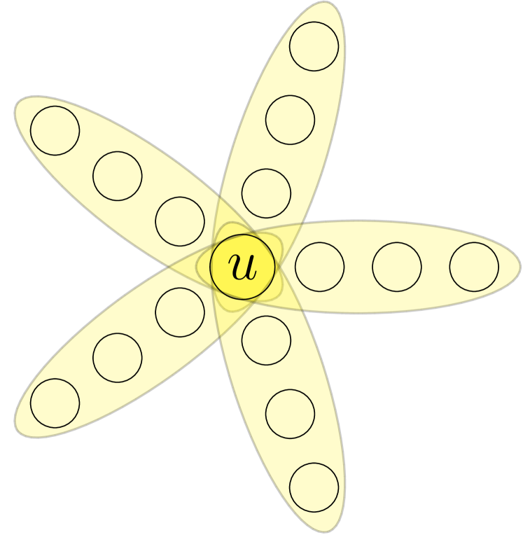
centrality	$c_{u}/c_{v}$	$\lim_{m\to\infty}c_{u}/c_{v}$
CEC	$\frac{2r(m-1)}{\sqrt{m^{2}+4(m-1)(r-1)}+m-2}$	$2r$
ZEC	$r^{1/2}$!$\ast$missing	$r^{1/2}$
HEC	$r^{1/m}$!	$1$

Figure 1: Hypergraph eigenvector centralities on sunflowers with singleton cores. (Left) A $4$-uniform, $5$-petal sunflower hypergraph with core $C=\{u\}$. Each petal is a hyperedge, marked here with a yellow-shaded ellipse around the nodes. (Right) Finite and asymptotic ratios of the centrality of the center node $u$ to any other node $v$ (which all have the same centrality) in a general $m$-uniform, $r$-petal sunflower hypergraph with singleton core. The ZEC scores have no dependence on $m$, and the HEC scores tend to uniform as $m$ grows.
$\ast$missingThis ratio holds when $m>3$ and can hold when $m=3$ (see Proposition 2.17).

A sunflower hypergraph has a hyperedge set $E$ with a common pairwise intersection. Formally, for any hyperedges (called petals) $A,B\in E$, $A\cap B=C$. The common intersection $C$ is called the core. The sunflower is similar to the star graph, which has been used to evaluate centralities in social networks [?]. Here, we use sunflowers as an illustrative example for the behavior of our three hypergraph eigenvector centralities. We specifically consider sunflowers with $r$ petals where the core is a singleton, i.e., $A\cap B=\{u\}$ for any $A,B\in E$ (Fig. 1, left). Below, we derive analytic solutions for the centrality of each method (see also Fig. 1, right). In all cases, the hypergraph centralities “do the right thing,” namely the center node $u$ has the largest centrality. However, the behavior of the three centralities differ.

CEC

Let $v$ be some other node than $u$. We assume that the centrality $c_{v}$ is equal to some constant $z$ for all nodes $v$ and show that we get a positive eigenvector. The Perron-Frobenius theorem then gives us uniqueness. Recall that $r$ is the number of petals in the hypergraph. Under these assumptions, the CEC equations satisfy

$$\textstyle\lambda c_{u} =\textstyle\sum_{(u,v_{1},\ldots,v_{m-1})\in E}\sum_{j=1}^{m-1}c_{v_{j}}\implies\lambda c_{u}=r(m-1)z$$

$$\lambda c_{v} =c_{u}+(m-2)z\implies\lambda^{2}z=r(m-1)z+\lambda(m-2)z$$

$$\implies\lambda=\textstyle\frac{1}{2}\sqrt{m^{2}+4(m-1)(r-1)}+m-2\implies c_{u}=\textstyle\frac{2r(m-1)}{\sqrt{m^{2}+4(m-1)(r-1)}+m-2}c_{v}$$

Since $m\geq 2$ and $c_{v}>0$, $c_{u}$ and $\lambda$ are both positive for any positive value $c_{v}$. Some algebra shows that $c_{u}>c_{v}$ for finite $m$ and $r\geq 2$:

$$\textstyle\frac{c_{u}}{c_{v}}=\frac{2r(m-1)}{\sqrt{m^{2}+4(m-1)(r-1)}+m-2}=\frac{r}{\sqrt{\frac{1}{4}\left(\frac{m}{m-1}\right)^{2}+\frac{r-1}{m-1}}+\frac{1}{2}\cdot\frac{m-2}{m-1}}>\frac{r}{\sqrt{1+\frac{r-1}{m-1}}+\frac{1}{2}}\geq\begin{cases}\frac{r}{\sqrt{2}+\frac{1}{2}}>1&m\geq r\\ \frac{r}{\sqrt{r}+\frac{1}{2}}>1&m<r\end{cases}.$$

Lastly, we only need to choose $c_{v}>0$ and normalize so that $\|\bm{\mathrm{c}}\|_{1}=1$.

ZEC

The Perron-Frobenius theorem for tensor $Z$-eigenvectors does not preclude the existence of multiple positive eigenvectors with positive eigenvalues. We indeed see the non-uniqueness for the sunflower, but only in the $3$-uniform case. We first show the following lemma, which states that the centrality of the non-core nodes in any petal must be the same.

Lemma 2.15.

In any sunflower whose common intersection is a singleton $\{u\}$, the ZEC scores of all nodes in the same petal—except for $u$—are the same.

Proof 2.16.

Let $c_{u}$ be the centrality score of node $u$. Let $w$ be any other node in an arbitrary petal $P$, whose centrality score is $c_{w}$. The ZEC equations satisfy

(10) $$\textstyle\lambda c_{w}=c_{u}\prod_{v\in P\backslash\{u,w\}}c_{v}\implies\lambda c_{w}^{2}=c_{u}\prod_{v\in P\backslash\{u\}}c_{v}=\lambda c_{w^{\prime}}^{2}\text{ for any $w^{\prime}\in P$missing}.$$

We next characterize exactly when the sunflower has a unique ZEC vector.

Proposition 2.17.

Let $\mathcal{H}$ be an $m$-uniform sunflower with singleton core $\{u\}$ and petals $\{P\}$.

1. If $m\neq 3$, the unique $Z$-eigenvector centrality score $\bm{\mathrm{c}}$ for $\mathcal{H}$ is given by $c_{u}/c_{v}=\sqrt{r}$, where $v$ is any node other than $u$ and $c_{v}$ is a constant over nodes $v\neq u$.

2. If $m=3$, there are infinite $Z$-eigenvector centrality scores for $\mathcal{H}$; any vector with $c_{v}=c_{P}$ for $v\in P,v\neq u$, and $c_{u}=\sqrt{\sum_{P}c_{P}^{2}}$ are $Z$-eigenvector centrality scores.

Proof 2.18.

By Lemma 2.15, each node other than $u$ has centrality $c_{P}$, where $P$ is the petal to which the node belongs. Re-writing Eq. 10 in terms of $c_{P}$ gives

(11) $$\textstyle\lambda c_{P}^{2}=c_{u}\prod_{v\in P\backslash\{u\}}c_{P}=c_{u}c_{P}^{m-1}\implies\lambda/c_{u}=c_{P}^{m-3}$$

This implies that $c_{P}^{m-3}=c_{P^{\prime}}^{m-3}$ for any petals $P$ and $P^{\prime}$. Assume $m\neq 3$. Then $c_{P}=c_{P^{\prime}}$ since $c_{P}>0$. Let $z$ be the centrality of any node $v\neq u$. The ZEC equations satisfy

(12) $$\lambda c_{u} =\textstyle\sum_{P}z^{m-1}=rz^{m-1}\text{ and }\lambda z=c_{u}z^{m-2}$$

Combining these equations gives $\lambda^{2}=rz^{2(m-2)}$, or $\lambda=\sqrt{r}z^{m-2}$. Plugging this expression for $\lambda$ into Eq. 12 gives

(13) $$\textstyle c_{u}/c_{v}=rz^{m-1}/(\lambda z)=rz^{m-1}/(\sqrt{r}z^{m-1})=\sqrt{r}.$$

Now assume $m=3$. Then $\lambda=c_{u}$ by Eq. 11. Let $c_{P}>0$ be an arbitrary constant for each petal $P$ and define $c_{u}^{2}=\sum_{P}c_{P}^{2}$. We now just check that the $Z$-eigenvector equations hold.

(14) $$\textstyle c_{u}^{2}=\lambda c_{u}=\sum_{P}\prod_{v\in P\backslash\{u\}}c_{v}=\sum_{P}c_{P}^{2},$$

which holds by the definition of $c_{u}^{2}$. Our choice of $c_{P}$ was any positive real number, and for any node $w\neq u$ in petal $P=\{u,v,w\}$, the ZEC equation is $c_{u}c_{P}=c_{u}c_{v}=\lambda c_{w}=c_{u}c_{w}=c_{u}c_{P}$.

Surprisingly, when $m=3$, the non-center nodes can have different ZEC scores, even though the symmetry of the problem would suggest that they would be the same. Also surprisingly, all scores are independent of $m$, the number of nodes in a hyperedge. However, ZEC is consistent in the sense that the center node always has the largest centrality score.

$H$-eigenvector centrality

Theorem 2.13 gives us uniqueness of a positive vector with positive eigenvalue. We again assume that $c_{v}=z$ for any node $v\neq u$. The HEC equations satisfy

(15) $$\textstyle\lambda c_{u}^{m-1} =\textstyle\sum_{(u,v_{1},\ldots,v_{m-1})}\prod_{j=1}^{m-1}c_{v_{j}}\implies\lambda c_{u}^{m-1}=rz^{m-1}$$

(16) $$\lambda c_{v}^{m-1} =c_{u}z^{m-2}\implies\lambda z^{m-1}=c_{u}z^{m-2}\implies c_{u}=\lambda z.$$

Plugging in $c_{u}=\lambda z$ into Eq. 15 gives $\lambda(\lambda z)^{m-1}=rz^{m-1}\implies\lambda=r^{1/m}$. Thus, $c_{u}/c_{v}=r^{1/m}$ for $v\neq u$, and $c_{u}/c_{v}\to 1$ if the number of petals $r$ is fixed and the uniformity $m$ grows large.

2.5 Recap: which centrality should we use?

We derived three hypergraph eigenvector centralities. The appeal of CEC is that we only need to rely on the familiar, i.e., we can just use nonnegative matrix theory. However, CEC does not incorporate any interesting nonlinear structure, whereas ZEC and HEC incorporate nonlinearity. HEC is certainly attractive computationally—simple algorithms can compute a unique eigenvector centrality vector. We don’t have scalable algorithms guaranteed to compute a ZEC vector, and even worse, the ZEC vector may not be unique. Moreover, the non-uniqueness can show up on simple hypergraphs, as we saw with the sunflower. Both CEC and HEC have a proper dimensional analysis, while ZEC does not. On the other hand, ZEC can carry the same rank-1 approximation interpretation as standard graph eigenvector centrality. Also, in the asymptotics of the sunflower analysis (Fig. 1, right), the HEC score of the center node approaches that of the other nodes, while the relative CEC and ZEC scores of the center node to the others are constants that only depend on the number of hyperedges.

So which centrality should we use? Our analysis suggests that none is superior to all others. As is the case with graph centralities in general, the scores are not useful in a vacuum. Instead, we can use various centralities to study data. For example, multiple centralities provide more features that can be used for machine learning tasks. In the next section, we show that the three hypergraph centralities can provide qualitatively different results on real-world data.

3 Computational experiments and data analysis

Table 1: Summary statistics of datasets. The number of nodes is the dimension of the cubic adjacency tensor $\mathchoice{\hbox to0.0pt{{$\underline{{\hbox to5.78613pt{}}}$\hss}}}{\hbox to0.0pt{{$\underline{{\hbox to5.78613pt{}}}$\hss}}}{\hbox to0.0pt{{$\underline{{\hbox to4.0503pt{}}}$\hss}}}{\hbox to0.0pt{{$\underline{{\hbox to2.89305pt{}}}$\hss}}}\bm{{T}}$ of the largest component of the hypergraph, and nnz($\mathchoice{\hbox to0.0pt{{$\underline{{\hbox to5.78613pt{}}}$\hss}}}{\hbox to0.0pt{{$\underline{{\hbox to5.78613pt{}}}$\hss}}}{\hbox to0.0pt{{$\underline{{\hbox to4.0503pt{}}}$\hss}}}{\hbox to0.0pt{{$\underline{{\hbox to2.89305pt{}}}$\hss}}}\bm{{T}}$) is the number of non-zeros in $\mathchoice{\hbox to0.0pt{{$\underline{{\hbox to5.78613pt{}}}$\hss}}}{\hbox to0.0pt{{$\underline{{\hbox to5.78613pt{}}}$\hss}}}{\hbox to0.0pt{{$\underline{{\hbox to4.0503pt{}}}$\hss}}}{\hbox to0.0pt{{$\underline{{\hbox to2.89305pt{}}}$\hss}}}\bm{{T}}$, which we divide by the number of symmetries in the symmetric tensor.

	​​​​​​​​​​​3-uniform		!!!!!!4-uniform		!!!!!!5-uniform
dataset	# nodes	$\frac{\text{nnz}(\mathchoice{\hbox to0.0pt{{$\underline{{\hbox to4.0503pt{}}}$\hss}}}{\hbox to0.0pt{{$\underline{{\hbox to4.0503pt{}}}$\hss}}}{\hbox to0.0pt{{$\underline{{\hbox to2.83519pt{}}}$\hss}}}{\hbox to0.0pt{{$\underline{{\hbox to2.02513pt{}}}$\hss}}}\bm{{T}})}{6}$	# nodes	$\frac{\text{nnz}(\mathchoice{\hbox to0.0pt{{$\underline{{\hbox to4.0503pt{}}}$\hss}}}{\hbox to0.0pt{{$\underline{{\hbox to4.0503pt{}}}$\hss}}}{\hbox to0.0pt{{$\underline{{\hbox to2.83519pt{}}}$\hss}}}{\hbox to0.0pt{{$\underline{{\hbox to2.02513pt{}}}$\hss}}}\bm{{T}})}{24}$	# nodes	$\frac{\text{nnz}(\mathchoice{\hbox to0.0pt{{$\underline{{\hbox to4.0503pt{}}}$\hss}}}{\hbox to0.0pt{{$\underline{{\hbox to4.0503pt{}}}$\hss}}}{\hbox to0.0pt{{$\underline{{\hbox to2.83519pt{}}}$\hss}}}{\hbox to0.0pt{{$\underline{{\hbox to2.02513pt{}}}$\hss}}}\bm{{T}})}{120}$
N-grams	30,885	888,411	23,713	957,904	24,996	995,952
tags-ask-ubuntu	2,981	279,369	2,856	145,676	2,564	25,475
DAWN	1,677	41,225	1,447	29,829	1,212	15,690

We now analyze our proposed eigenvector centralities on three real-world datasets. We construct a 3-uniform, 4-uniform, and 5-uniform hypergraph from each of the three datasets (summary statistics are in Table 1), so there are 9 total hypergraphs for our analysis. For each of the 9 hypergraphs, we computed the CEC, ZEC, and HEC scores on the largest connected component of the hypergraph. We used Julia’s eigs routine to compute the CEC scores, the dynamical systems algorithm by ? to compute the ZEC scores, and the NQI algorithm [?] to compute the HEC scores. The software used to compute the results in this section is available at https://github.com/arbenson/Hyper-Evec-Centrality.

As discussed above, the ZEC vector need not be unique. We computed 100 ZEC vectors using random starting points and found that, for some datasets, the algorithm always converges to the same eigenvector and in others, the algorithm converges to a few different ones. For the purposes of our analysis, we use the ZEC vector to which convergence was most common. However, any of the ZEC vectors is a valid centrality. (One could also possibly take the mean of several ZEC vectors, but linear combinations of $Z$-eigenvectors are not necessarily $Z$-eigenvectors, unlike the matrix case.)

N-grams

These hypergraphs are constructed from the most frequent $N$-grams in the Corpus of Contemporary American English (COCA) [?]. An $N$-gram is a sequence of $N$ words (or parts of words, but we will just say “words”) that appear contiguously in text. Here, we use the million most frequent $N$-grams dataset from COCA for $N=3,4,5$ to compose hyperedges. We construct $m$-uniform hypergraphs ($m=3,4,5$) as follows. The set of nodes in the $m$-uniform hypergraph correspond to all words appearing in at least one of the $m$-grams in the corpus. There is a hyperedge between $m$ nodes if the corresponding $m$ words (appearing in any permutation order) make up one of the $m$-grams appearing in the corpus. For each hypergraph, we analyze its largest connected component, which is given by taking the node set $L$ from the largest connected component of the graph discussed in Definition 2.2, and only keeping the hyperedges comprised entirely of nodes in $L$.

Section 3 lists the top 20 ranked words according to the CEC, ZEC, and HEC scores for each of the three hypergraphs. Many of the top-ranked words are so-called stop words, such as “the,” “and,” and “to”; furthermore, nearly all of the top 20 ranked words for CEC and HEC are stop words or conjunctions, regardless of the size of the $N$-gram. This is perhaps not surprising, given that stop words are by definition common in natural language (stop words also form important clusters in tensor-based clustering of $N$-gram data [?]). The same is true of the ZEC scores, but only for the 3-grams and 4-grams. In the 5-uniform hypergraph, the word “world” has rank 12 with ZEC, rank 64 with CEC, and rank 84 with HEC; and the word “people” has rank 14 with ZEC, rank 39 with CEC, and rank 44 with HEC.

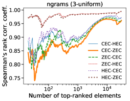
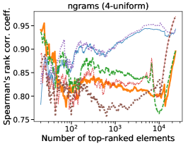
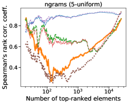
Figure 2: Spearman’s rank correlation coefficient between the top $k$ ranked nodes from one centrality measure with the same nodes from the other two centrality measures on the $N$-grams dataset (the one used to determine the nodes is listed first in the legend). The rank correlation for the top few hundred nodes with ZEC and the other centralities decreases as the uniformity of the hypergraph increases, and dips below 0.4 for the 5-uniform hypergraph.

To better quantify the relationship between the centralities, we computed the Spearman’s rank correlation coefficient between components of each centrality vector. Specifically, for each of CEC, ZEC, and HEC, we find the top $k$ ranked nodes and compute the rank correlation on the sub-vectors consisting of these nodes with the other two centrality vectors. For example, if $k=100$, we compute the top 100 nodes according to the CEC vector, take the length-100 sub-vector corresponding to the same nodes in the ZEC vector, and compute the rank correlation between the vectors. This is repeated for all six possible pairs of vectors and plotted as a function of $k$ (Fig. 2).

As a function of $k$, the rank correlations in this dataset tend to have local minima for $k$ between 20 and a few hundred. Larger values of $k$ catch the tail of the distribution for which there is less difference in ranking, which leads to the increase in the correlation for large $k$. We also see that the correlations tend to decrease as we increase the uniformity of the hypergraph. In other words, the three centrality measures become more different when considering larger multi-way relationships. Finally, the rank correlations reveal that ZEC ranks the top nodes (beyond the top 20) substantially differently than CEC and HEC.

tags-ask-ubuntu

Ask Ubuntu is a Stack Exchange forum, where Ubuntu users and developers ask, answer, and discuss questions. Each question may be annotated with up to five tags to aid in classification. We construct 3-uniform, 4-uniform, and 5-uniform hypergraphs from a previously collected dataset of tag co-appearances in questions [?]. Specifically, the nodes of the hypergraphs represent tags. We add each possible hyperedge to the $m$-uniform hypergraph if the corresponding $m$ tags were all simultaneously used to annotate at least one question on the web site (the question could also have contained other tags; for constructing the hyperedge, we only care if the $m$ tags were used for the question). Finally, as before, we use the largest component of the hypergraph.

Section 3 lists the top 10 nodes ranked by CEC, ZEC, HEC for each of the three hypergraphs. With the 3-uniform hypergraph, these top-ranked nodes are roughly the same for each centrality measure, with major Ubuntu version numbers (“12.04,” “14.04,” and “16.04”) near or at the top of each list. When moving to 4-uniform and 5-uniform hypergraphs, the version numbers remain highly ranked, but not the most highly ranked. ZEC finds tags related to the Windows operating system relatively more important. For example, the tags “windows-8”, “windows”, and “windows-7” are ranked 8, 9, and 10 with ZEC for the 5-uniform hypergraph but ranked 28, 22, and 26 with CEC and 21, 18, and 20 with HEC. Furthermore, ZEC ranks “windows,” “windows-xp,” “windows-vista,” “windows-7,” “windows-8,” and “windows-10” higher than CEC and HEC for all three hypergraphs. We conclude that ZEC provides complimentary information to the centralities for this dataset.

Figure 3 lists the same rank correlations as described above. We again see that all centrality vectors are relatively correlated for the 3-uniform hypergraph but less so as we increase the order of the hypergraph. The sub-vector corresponding to the top 10 ranked CEC nodes has only 0.05 rank correlation with the same ZEC sub-vector for the 4-uniform hypergraph.

DAWN

The Drug Abuse Warning Network (DAWN) is a national health surveillance system in hospitals throughout the United States that records the drug use reported by patients visiting emergency rooms. Here, drugs include illicit substances, prescription medication, over-the-counter medication, and dietary supplements. We use a dataset that aggregates 8 years of DAWN reports [?] to construct $m$-uniform hypergraphs for $m=3,4,5$. The nodes in each hypergraph correspond to drugs. We add a hyperedge on $m$ nodes if there is at least one patient that reports using exactly that combination of $m$ drugs. Again, we use the largest component of the hypergraph.

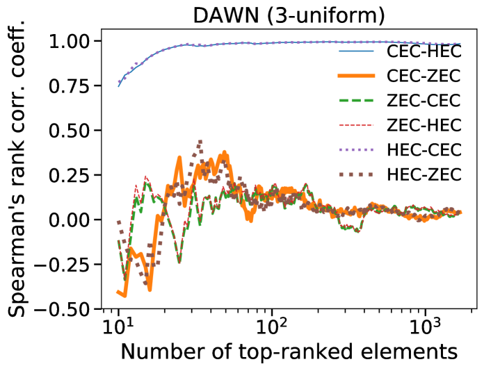
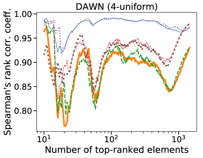
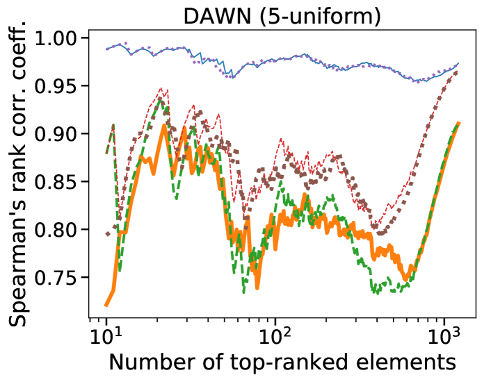
Figure 4: Spearman’s rank correlation coefficient between the top $k$ ranked nodes from one centrality measure with the same nodes from the other two centrality measures on the DAWN dataset (the one used to determine the nodes is listed first in the legend). ZEC is negatively or nearly uncorrelated with CEC and HEC for the 3-uniform hypergraph, but all centralities are quite positively correlated for the 4-uniform and 5-uniform hypergraphs, which can also be observed from the similar top 10 nodes listed in Section 3 (left).

We again list the top 10 ranked nodes by the three centrality vectors for each of the three hypergraphs (Section 3) as well as the same rank correlation statistics (Fig. 4). In this dataset, we see near agreement between the three centrality vectors across the 4-uniform and 5-uniform hypergraphs. For example, the rank correlations remain above 0.75 for the entire 4-uniform hypergraph for all measured top $k$ sub-vectors. Alcohol is consistently ranked near the top, which is unsurprising given its pervasiveness in emergency department visits, especially in combination with other drugs [?].

The ranking from the ZEC vector is substantially different from HEC and CEC for the 3-uniform hypergraph. Leading sub-vectors of ZEC actually have negative rank correlation with the corresponding HEC and CEC sub-vectors. As with the N-grams and tags-ask-ubuntu datasets, we again conclude that ZEC provides complimentary information for the centralities.

Table 2: Top 20 nodes with largest centralities for CEC, ZEC, and HEC for the three hypergraphs constructed from the frequent $n$-grams. Many stop words appear as the top-ranked nodes, but ZEC picks up on non-stop words such as “world” and “people” on the hypergraph constructed from frequent $5$-grams.

	3-uniform			4-uniform			5-uniform
	CEC	ZEC	HEC	CEC	ZEC	HEC	CEC	ZEC	HEC
1	the	the	the	the	the	the	the	the	the
2	of	to	to	of	of	to	of	of	to
3	in	and	a	to	to	of	to	in	of
4	and	a	and	in	in	a	in	and	a
5	to	that	of	a	and	in	a	to	that
6	a	in	in	and	that	that	and	that	in
7	that	of	that	that	a	and	that	on	and
8	on	is	for	on	is	is	is	is	i
9	for	for	is	is	on	it	on	a	it
10	with	it	on	for	for	was	be	one	n’t
11	is	on	was	was	was	i	for	for	is
12	was	was	with	be	it	you	was	world	you
13	from	with	it	with	you	have	it	with	have
14	at	you	as	it	with	be	have	people	was
15	by	this	you	at	one	for	i	end	be
16	as	as	i	have	be	on	with	part	do
17	his	i	this	i	have	he	at	at	he
18	it	have	be	as	all	n’t	you	first	for
19	be	at	have	he	this	with	n’t	rest	on
20	are	not	at	you	at	not	as	was	we

Table 3: Top 10 nodes with largest centralities for CEC, ZEC, and HEC for three hypergraphs constructed from the co-tagging dataset tags-ask-ubuntu. These highly-ranked nodes are largely the same in the 3-uniform hypergraph. For the 4-uniform and 5-uniform hypergraphs, ZEC picks up on Windows-related tags. Tags related to version numbers are ranked lower as the uniformity of the hypergraph increases.

		CEC	ZEC	HEC
3-uniform	1	14.04	14.04	14.04
	2	12.04	12.04	12.04
	3	16.04	boot	16.04
	4	server	16.04	boot
	5	command-line	drivers	drivers
	6	boot	nvidia	command-line
	7	networking	dual-boot	server
	8	drivers	server	networking
	9	unity	command-line	unity
	10	gnome	upgrade	gnome
		CEC	ZEC	HEC
4-uniform	1	14.04	dual-boot	14.04
	2	boot	boot	boot
	3	drivers	grub2	drivers
	4	12.04	partitioning	12.04
	5	16.04	uefi	16.04
	6	networking	system-installation	dual-boot
	7	server	14.04	nvidia
	8	dual-boot	windows	grub2
	9	nvidia	installation	networking
	10	grub2	12.04	partitioning
		CEC	ZEC	HEC
5-uniform	1	boot	dual-boot	boot
	2	dual-boot	boot	dual-boot
	3	14.04	grub2	grub2
	4	drivers	partitioning	drivers
	5	grub2	uefi	14.04
	6	networking	system-installation	partitioning
	7	16.04	14.04	nvidia
	8	partitioning	windows-8	16.04
	9	nvidia	windows	12.04
	10	12.04	windows-7	networking

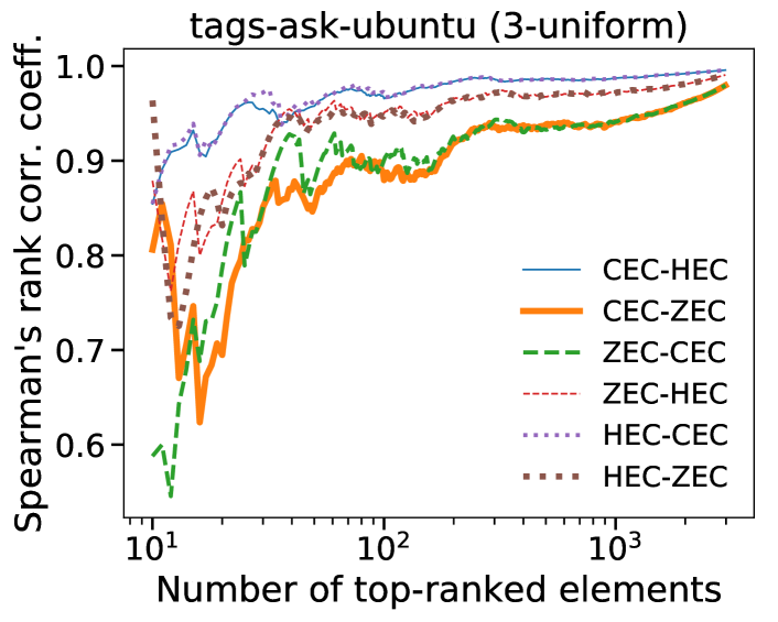
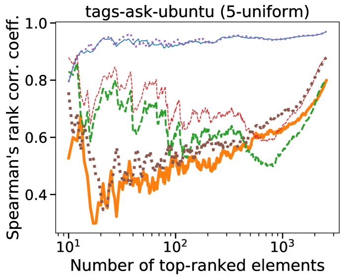
Figure 3: Spearman’s rank correlation coefficient between the top $k$ ranked nodes from one centrality measure with the same nodes from the other two centrality measures on the Ask Ubuntu co-tagging dataset (the one used to determine the nodes is listed first in the legend). For the 3-uniform hypergraph, all centralities are relatively correlated for $k\geq 30$. For the 4-uniform and 5-uniform hypergraphs, ZEC tends to be less correlated with CEC and HEC, which is also seen in the rankings of the top 10 nodes (Section 3, left).

Table 4: Top 10 nodes with largest centralities for CEC, ZEC, and HEC for three hypergraphs constructed from the reported sets of drugs used by patients in emergency room visits in the DAWN dataset. The highly-ranked nodes in the 4-uniform and 5-uniform hypergraphs are largely the same and are consistent across the centrality measures.

		CEC	ZEC	HEC
3-uniform	1	alcohol	cephalothin	alcohol
	2	cocaine	naloxone	alprazolam
	3	marijuana	meclizine	acet.-hydrocodone
	4	acet.-hydrocodone	cyclosporine	clonazepam
	5	alprazolam	desipramine	cocaine
	6	clonazepam	donnatal elixir	marijuana
	7	ibuprofen	pyridostigmine	quetiapine
	8	quetiapine	amoxapine	lorazepam
	9	acetaminophen	aspirin	ibuprofen
	10	lorazepam	bicalutamide	zolpidem
	1	alcohol	alcohol	alcohol
	2	cocaine	cocaine	cocaine
	3	marijuana	marijuana	marijuana
	4	alprazolam	alprazolam	alprazolam
	5	acet.-hydrocodone	acet.-hydrocodone	acet.-hydrocodone
	6	clonazepam	clonazepam	clonazepam
	7	quetiapine	heroin	quetiapine
	8	heroin	oxycodone	oxycodone
	9	oxycodone	methadone	heroin
	10	lorazepam	acet.-oxycodone	acet.-oxycodone
	1	alcohol	cocaine	alcohol
	2	cocaine	alcohol	cocaine
	3	marijuana	marijuana	marijuana
	4	alprazolam	heroin	alprazolam
	5	acet.-hydrocodone	alprazolam	acet.-hydrocodone
	6	clonazepam	benzodiazepines	heroin
	7	heroin	oxycodone	clonazepam
	8	benzodiazepines	acet.-hydrocodone	benzodiazepines
	9	oxycodone	methadone	oxycodone
	10	narcotic analgesics	narcotic analgesics	narcotic analgesics

4 Discussion

Centrality is a pillar of network science, and emerging datasets containing supra-dyadic relationships offer new challenges in understanding centrality in complex systems. Here, we proposed three eigenvector centralities for hypergraph models of such multi-relational data. Two of these incorporated non-linear structure and relied on fairly recent developments in the spectral theory of tensors to create a sensible definition. None of the three centralities is “best” and we saw empirically that the eigenvectors can provide qualitatively different results. There are several other types of tensor eigenvectors [?], as well as other types of Perron-Frobenius theorems for hypergraph data [?], which could be adapted for new centrality measures. However, $Z$- and $H$-eigenvectors are arguably the most well-understood and commonly used tensor eigenvectors.

There are other centrality measures and ranking methods for higher-order relational data. For example, multilinear PageRank generalizes PageRank to tensors [??]. ? developed eigenvector centrality for multiplex networks using new Perron-Frobenius theory of multi-linear maps [?]; this is most similar to HEC. There are also several ranking methods for multi-relational data represented as tensors [????], as well as notions of centrality based on simplicial complexes [?]. Finally, there are other centralitities for hypergraphs [?????], but these do not relate to the multilinear structure of tensors that we studied.

We used a set-based definition of hypergraphs that made the adjacency tensor symmetric. In network science, directed graphs with non-symmetric adjacency matrices are a common model, and eigenvector centrality is still well-defined if the graph is strongly connected. There are similar notions of directionality in hypergraphs. For example, the N-grams dataset could have been interpreted as “directed” since the ordering of the words matters for its frequency. Trajectory or path-based data appearing in transportation systems [?], citation patterns [?], and human contact sequences [?] can be encoded as directed hypergraphs in similar ways. Theorems 2.6 and 2.13 hold for arbitrary irreducible nonnegative tensors, which includes adjacency tensors of strongly connected hypergraphs. Therefore, the hypergraph centralities we developed remain well-defined in these more general cases. However, computation becomes a bigger challenge.

There are many choices in deciding how to construct hypergraphs from data. As one example, we made our adjacency tensors binary (i.e., an unweighted hypergraph). This was not necessary mathematically, and all of the proposed methods work seamlessly if the hypergraph is weighted. The Ask Ubuntu and DAWN datasets also demonstrated two different ways of constructing hyperedges—in the former we included hyperedges induced by larger sets and in the latter we did not. This choice was made to illustrate the point that there are several ways one could construct hypergraphs from data. Our methods also relied on theory for symmetric tensors, so we studied uniform hypergraphs. One could incorporate non-uniformity in several ways. A simple approach could combine the scores for hypergraphs of different uniformity. We could also “embed” smaller hyperedges into a larger adjacency tensor. For example, a mixture of 3-node and 4-node hyperedges could be incorporated into an order-4 adjacency tensor, where a 3-node hyperedge $\{i,j,k\}$ adds non-zeros in the indices that only contain $i$, $j$, and $k$ (e.g., setting $\mathchoice{\hbox to0.0pt{{$\underline{{\hbox to5.78613pt{}}}$\hss}}}{\hbox to0.0pt{{$\underline{{\hbox to5.78613pt{}}}$\hss}}}{\hbox to0.0pt{{$\underline{{\hbox to4.0503pt{}}}$\hss}}}{\hbox to0.0pt{{$\underline{{\hbox to2.89305pt{}}}$\hss}}}\bm{{T}}_{ijkk}=1$ would create one such non-zero). In general, hypergraphs can be a convenient abstraction, and understanding the right way of constructing a hypergraph from data is a general research challenge.

Bibliography

- Agarwal et al. (2006) S. Agarwal, K. Branson, and S. Belongie. Higher order learning with graphs. In Proceedings of the 23rd international conference on Machine learning. 2006. doi:10.1145/1143844.1143847.
- Balasubramaniam et al. (2016) K. Balasubramaniam, B. Beisner, J. Vandeleest, E. Atwill, and B. McCowan. Social buffering and contact transmission: network connections have beneficial and detrimental effects on Shigella infection risk among captive rhesus macaques. PeerJ, 4, p. e2630, 2016. doi:10.7717/peerj.2630.
- Bavelas (1950) A. Bavelas. Communication patterns in task-oriented groups. The Journal of the Acoustical Society of America, 22 (6), pp. 725–730, 1950. doi:10.1121/1.1906679.
- Benson et al. (2018) A. R. Benson, R. Abebe, M. T. Schaub, A. Jadbabaie, and J. Kleinberg. Simplicial closure and higher-order link prediction. arXiv:1802.06916, 2018.
- Benson and Gleich (2018) A. R. Benson and D. F. Gleich. Computing tensor Z-eigenvectors with dynamical systems. arXiv:1805.00903, 2018.
- Benson et al. (2016) A. R. Benson, D. F. Gleich, and J. Leskovec. Higher-order organization of complex networks. Science, 353 (6295), pp. 163–166, 2016. doi:10.1126/science.aad9029.
- Benson et al. (2017) A. R. Benson, D. F. Gleich, and L.-H. Lim. The spacey random walk: A stochastic process for higher-order data. SIAM Review, 59 (2), pp. 321–345, 2017. doi:10.1137/16m1074023.
- Benzi and Klymko (2015) M. Benzi and C. Klymko. On the limiting behavior of parameter-dependent network centrality measures. SIAM Journal on Matrix Analysis and Applications, 36 (2), pp. 686–706, 2015. doi:10.1137/130950550.
- Berge (1984) C. Berge. Hypergraphs: combinatorics of finite sets, Elsevier, 1984.
- Berman and Plemmons (1994) A. Berman and R. J. Plemmons. Nonnegative matrices in the mathematical sciences, SIAM, 1994.
- Boldi and Vigna (2014) P. Boldi and S. Vigna. Axioms for centrality. Internet Mathematics, 10 (3-4), pp. 222–262, 2014. doi:10.1080/15427951.2013.865686.
- Bonacich (1972) P. Bonacich. Technique for analyzing overlapping memberships. Sociological Methodology, 4, p. 176, 1972. doi:10.2307/270732.
- Bonacich (1987) ———. Power and centrality: A family of measures. American Journal of Sociology, 92 (5), pp. 1170–1182, 1987. doi:10.1086/228631.
- Bonacich et al. (2004) P. Bonacich, A. C. Holdren, and M. Johnston. Hyper-edges and multidimensional centrality. Social Networks, 26 (3), pp. 189–203, 2004. doi:10.1016/j.socnet.2004.01.001.
- Borgatti and Everett (2006) S. P. Borgatti and M. G. Everett. A graph-theoretic perspective on centrality. Social Networks, 28 (4), pp. 466–484, 2006. doi:10.1016/j.socnet.2005.11.005.
- Brin and Page (1998) S. Brin and L. Page. The anatomy of a large-scale hypertextual web search engine. Computer Networks and ISDN Systems, 30 (1-7), pp. 107–117, 1998. doi:10.1016/s0169-7552(98)00110-x.
- Bryan and Leise (2006) K. Bryan and T. Leise. The $25,000,000,000 eigenvector: The linear algebra behind google. SIAM Review, 48 (3), pp. 569–581, 2006. doi:10.1137/050623280.
- Bullmore and Sporns (2009) E. Bullmore and O. Sporns. Complex brain networks: graph theoretical analysis of structural and functional systems. Nature Reviews Neuroscience, 10 (3), pp. 186–198, 2009. doi:10.1038/nrn2575.
- Busseniers (2014) E. Busseniers. General centrality in a hypergraph. arXiv:1403.5162, 2014.
- Chang et al. (2013) K. Chang, K. Pearson, and T. Zhang. Some variational principles for -eigenvalues of nonnegative tensors. Linear Algebra and its Applications, 438 (11), pp. 4166–4182, 2013. doi:10.1016/j.laa.2013.02.013.
- Chang et al. (2008) K. C. Chang, K. Pearson, and T. Zhang. Perron-frobenius theorem for nonnegative tensors. Communications in Mathematical Sciences, 6 (2), pp. 507–520, 2008. doi:10.4310/cms.2008.v6.n2.a12.
- Chen et al. (2012) B. Chen, S. He, Z. Li, and S. Zhang. Maximum block improvement and polynomial optimization. SIAM Journal on Optimization, 22 (1), pp. 87–107, 2012. doi:10.1137/110834524.
- Crane (2013) E. H. Crane. Highlights of the 2011 drug abuse warning network (dawn) findings on drug-related emergency department visits. 2013.
- Cui et al. (2014) C.-F. Cui, Y.-H. Dai, and J. Nie. All real eigenvalues of symmetric tensors. SIAM Journal on Matrix Analysis and Applications, 35 (4), pp. 1582–1601, 2014. doi:10.1137/140962292.
- Davies (2011) M. Davies. N-grams data from the Corpus of Contemporary American English (COCA). 2011.
- de Sola Pool and Kochen (1978) I. de Sola Pool and M. Kochen. Contacts and influence. Social Networks, 1 (1), pp. 5–51, 1978. doi:10.1016/0378-8733(78)90011-4.
- Estrada and Higham (2010) E. Estrada and D. J. Higham. Network properties revealed through matrix functions. SIAM Review, 52 (4), pp. 696–714, 2010. doi:10.1137/090761070.
- Estrada and Rodríguez-Velázquez (2006) E. Estrada and J. A. Rodríguez-Velázquez. Subgraph centrality and clustering in complex hyper-networks. Physica A: Statistical Mechanics and its Applications, 364, pp. 581–594, 2006. doi:10.1016/j.physa.2005.12.002.
- Estrada and Ross (2018) E. Estrada and G. J. Ross. Centralities in simplicial complexes. applications to protein interaction networks. Journal of Theoretical Biology, 438, pp. 46–60, 2018. doi:10.1016/j.jtbi.2017.11.003.
- Franz et al. (2009) T. Franz, A. Schultz, S. Sizov, and S. Staab. TripleRank: Ranking semantic web data by tensor decomposition. In Lecture Notes in Computer Science, pp. 213–228. Springer Berlin Heidelberg, 2009. doi:10.1007/978-3-642-04930-9_14.
- Freeman (1977) L. C. Freeman. A set of measures of centrality based on betweenness. Sociometry, 40 (1), p. 35, 1977. doi:10.2307/3033543.
- Friedland and Ottaviani (2014) S. Friedland and G. Ottaviani. The number of singular vector tuples and uniqueness of best rank-one approximation of tensors. Foundations of Computational Mathematics, 14 (6), pp. 1209–1242, 2014. doi:10.1007/s10208-014-9194-z.
- Gallo et al. (1993) G. Gallo, G. Longo, S. Pallottino, and S. Nguyen. Directed hypergraphs and applications. Discrete Applied Mathematics, 42 (2-3), pp. 177–201, 1993. doi:10.1016/0166-218x(93)90045-p.
- Gautier et al. (2017) A. Gautier, F. Tudisco, and M. Hein. The perron-frobenius theorem for multi-homogeneous maps. arXiv:1702.03230, 2017.
- Gautier et al. (2018) ———. A unifying perron-frobenius theorem for nonnegative tensors via multi-homogeneous maps. arXiv:1801.04215, 2018.
- Gleich (2015) D. F. Gleich. PageRank beyond the web. SIAM Review, 57 (3), pp. 321–363, 2015. doi:10.1137/140976649.
- Gleich et al. (2015) D. F. Gleich, L.-H. Lim, and Y. Yu. Multilinear PageRank. SIAM Journal on Matrix Analysis and Applications, 36 (4), pp. 1507–1541, 2015. doi:10.1137/140985160.
- Golub and Van Loan (2013) G. H. Golub and C. F. Van Loan. Matrix computations, JHU press, 4 edition, 2013.
- Henderson et al. (2012) K. Henderson, B. Gallagher, T. Eliassi-Rad, H. Tong, S. Basu, L. Akoglu, D. Koutra, C. Faloutsos, and L. Li. RolX: structural role extraction & mining in large graphs. In Proceedings of the 18th ACM SIGKDD international conference on Knowledge discovery and data mining. 2012. doi:10.1145/2339530.2339723.
- Hillar and Lim (2013) C. J. Hillar and L.-H. Lim. Most tensor problems are NP-hard. Journal of the ACM, 60 (6), pp. 1–39, 2013. doi:10.1145/2512329.
- Jeong et al. (2001) H. Jeong, S. P. Mason, A.-L. Barabási, and Z. N. Oltvai. Lethality and centrality in protein networks. Nature, 411 (6833), pp. 41–42, 2001. doi:10.1038/35075138.
- Kapoor et al. (2013) K. Kapoor, D. Sharma, and J. Srivastava. Weighted node degree centrality for hypergraphs. In 2013 IEEE 2nd Network Science Workshop (NSW). 2013. doi:10.1109/nsw.2013.6609212.
- Katz (1953) L. Katz. A new status index derived from sociometric analysis. Psychometrika, 18 (1), pp. 39–43, 1953. doi:10.1007/bf02289026.
- Kleinberg (1999) J. M. Kleinberg. Authoritative sources in a hyperlinked environment. Journal of the ACM, 46 (5), pp. 604–632, 1999. doi:10.1145/324133.324140.
- Kofidis and Regalia (2002) E. Kofidis and P. A. Regalia. On the best rank-1 approximation of higher-order supersymmetric tensors. SIAM Journal on Matrix Analysis and Applications, 23 (3), pp. 863–884, 2002. doi:10.1137/s0895479801387413.
- Kolda and Bader (2006) T. Kolda and B. Bader. The TOPHITS model for higher-order web link analysis. In Proceedings of Link Analysis, Counterterrorism and Security 2006. 2006.
- Kolda et al. (2005) T. Kolda, B. Bader, and J. Kenny. Higher-order web link analysis using multilinear algebra. In Fifth IEEE International Conference on Data Mining. 2005. doi:10.1109/icdm.2005.77.
- Kolda and Bader (2009) T. G. Kolda and B. W. Bader. Tensor decompositions and applications. SIAM Review, 51 (3), pp. 455–500, 2009. doi:10.1137/07070111X.
- Kolda and Mayo (2011) T. G. Kolda and J. R. Mayo. Shifted power method for computing tensor eigenpairs. SIAM Journal on Matrix Analysis and Applications, 32 (4), pp. 1095–1124, 2011. doi:10.1137/100801482.
- Kolda and Mayo (2014) ———. An adaptive shifted power method for computing generalized tensor eigenpairs. SIAM Journal on Matrix Analysis and Applications, 35 (4), pp. 1563–1581, 2014. doi:10.1137/140951758.
- Koutra et al. (2013) D. Koutra, J. T. Vogelstein, and C. Faloutsos. DeltaCon: A principled massive-graph similarity function. In Proceedings of the 2013 SIAM International Conference on Data Mining, pp. 162–170. Society for Industrial and Applied Mathematics, 2013. doi:10.1137/1.9781611972832.18.
- Lathauwer et al. (2000) L. D. Lathauwer, B. D. Moor, and J. Vandewalle. On the Best Rank- and Rank-(, , , ) Approximation of Higher-Order Tensors. SIAM Journal on Matrix Analysis and Applications, 21 (4), pp. 1324–1342, 2000. doi:10.1137/s0895479898346995.
- Lim (2005) L.-H. Lim. Singular values and eigenvalues of tensors: A variational approach. In First IEEE International Workshop on Computational Advances in Multi-Sensor Adaptive Processing. 2005. doi:10.1109/camap.2005.1574201.
- Lim (2013) ———. Tensors and hypermatrices. In Handbook of Linear Algebra, Second Edition, chapter 15, pp. 231–260. Chapman and Hall/CRC, 2013. doi:10.1201/b16113-19.
- Liu et al. (2010) Y. Liu, G. Zhou, and N. F. Ibrahim. An always convergent algorithm for the largest eigenvalue of an irreducible nonnegative tensor. Journal of Computational and Applied Mathematics, 235 (1), pp. 286–292, 2010. doi:10.1016/j.cam.2010.06.002.
- Lohmann et al. (2010) G. Lohmann, D. S. Margulies, A. Horstmann, B. Pleger, J. Lepsien, D. Goldhahn, H. Schloegl, M. Stumvoll, A. Villringer, and R. Turner. Eigenvector centrality mapping for analyzing connectivity patterns in fMRI data of the human brain. PLOS ONE, 5 (4), p. e10232, 2010. doi:10.1371/journal.pone.0010232.
- Lovász (2007) L. Lovász. Eigenvalues of graphs. 2007.
- Michoel and Nachtergaele (2012) T. Michoel and B. Nachtergaele. Alignment and integration of complex networks by hypergraph-based spectral clustering. Physical Review E, 86 (5), 2012. doi:10.1103/physreve.86.056111.
- Newman (2003) M. E. J. Newman. The structure and function of complex networks. SIAM Review, 45 (2), pp. 167–256, 2003. doi:10.1137/s003614450342480.
- Newman (2008) ———. Mathematics of networks. In The New Palgrave Encyclopedia of Economics. Palgrave Macmillan, Basingstoke, second edition, 2008.
- Ng et al. (2010) M. Ng, L. Qi, and G. Zhou. Finding the largest eigenvalue of a nonnegative tensor. SIAM Journal on Matrix Analysis and Applications, 31 (3), pp. 1090–1099, 2010. doi:10.1137/09074838x.
- Ng et al. (2011) M. K.-P. Ng, X. Li, and Y. Ye. MultiRank: co-ranking for objects and relations in multi-relational data. In Proceedings of the 17th ACM SIGKDD international conference on Knowledge discovery and data mining. 2011. doi:10.1145/2020408.2020594.
- Nie and Wang (2014) J. Nie and L. Wang. Semidefinite relaxations for best rank-1 tensor approximations. SIAM Journal on Matrix Analysis and Applications, 35 (3), pp. 1155–1179, 2014. doi:10.1137/130935112.
- Nie and Zhang (2017) J. Nie and X. Zhang. Real eigenvalues of nonsymmetric tensors. Computational Optimization and Applications, 70 (1), pp. 1–32, 2017. doi:10.1007/s10589-017-9973-y.
- Page et al. (1999) L. Page, S. Brin, R. Motwani, and T. Winograd. The pagerank citation ranking: Bringing order to the web. Technical report, Stanford InfoLab, 1999.
- Qi (2005) L. Qi. Eigenvalues of a real supersymmetric tensor. Journal of Symbolic Computation, 40 (6), pp. 1302–1324, 2005. doi:10.1016/j.jsc.2005.05.007.
- Qi and Luo (2017) L. Qi and Z. Luo. Tensor analysis: Spectral theory and special tensors, SIAM, 2017.
- Qi et al. (2016) Y. Qi, P. Comon, and L.-H. Lim. Uniqueness of nonnegative tensor approximations. IEEE Transactions on Information Theory, 62 (4), pp. 2170–2183, 2016. doi:10.1109/tit.2016.2532906.
- Regalia and Kofidis (2000) P. A. Regalia and E. Kofidis. The higher-order power method revisited: convergence proofs and effective initialization. In Proceedings of the IEEE International Conference on Acoustics, Speech, and Signal Processing. 2000. doi:10.1109/icassp.2000.861047.
- Rodríguez et al. (2007) J. A. Rodríguez, E. Estrada, and A. Gutiérrez. Functional centrality in graphs. Linear and Multilinear Algebra, 55 (3), pp. 293–302, 2007. doi:10.1080/03081080601002221.
- Rosvall et al. (2014) M. Rosvall, A. V. Esquivel, A. Lancichinetti, J. D. West, and R. Lambiotte. Memory in network flows and its effects on spreading dynamics and community detection. Nature Communications, 5 (1), 2014. doi:10.1038/ncomms5630.
- Ruhnau (2000) B. Ruhnau. Eigenvector-centrality — a node-centrality? Social Networks, 22 (4), pp. 357–365, 2000. doi:10.1016/s0378-8733(00)00031-9.
- Sabidussi (1966) G. Sabidussi. The centrality index of a graph. Psychometrika, 31 (4), pp. 581–603, 1966. doi:10.1007/bf02289527.
- Scholtes (2017) I. Scholtes. When is a network a network? multi-order graphical model selection in pathways and temporal networks. In Proceedings of the 23rd ACM SIGKDD International Conference on Knowledge Discovery and Data Mining. 2017. doi:10.1145/3097983.3098145.
- Strogatz (2001) S. H. Strogatz. Exploring complex networks. Nature, 410 (6825), pp. 268–276, 2001. doi:10.1038/35065725.
- Taylor et al. (2017) D. Taylor, S. A. Myers, A. Clauset, M. A. Porter, and P. J. Mucha. Eigenvector-based centrality measures for temporal networks. Multiscale Modeling & Simulation, 15 (1), pp. 537–574, 2017. doi:10.1137/16m1066142.
- Tudisco et al. (2018) F. Tudisco, F. Arrigo, and A. Gautier. Node and layer eigenvector centralities for multiplex networks. SIAM Journal on Applied Mathematics, 78 (2), pp. 853–876, 2018. doi:10.1137/17m1137668.
- Wu et al. (2016) T. Wu, A. R. Benson, and D. F. Gleich. General tensor spectral co-clustering for higher-order data. In Advances in Neural Information Processing Systems, pp. 2559–2567. 2016.
- Xu et al. (2016) J. Xu, T. L. Wickramarathne, and N. V. Chawla. Representing higher-order dependencies in networks. Science Advances, 2 (5), pp. e1600028–e1600028, 2016. doi:10.1126/sciadv.1600028.
- Ye and Akoglu (2015) J. Ye and L. Akoglu. Discovering opinion spammer groups by network footprints. In Proceedings of the 2015 ACM on Conference on Online Social Networks. 2015. doi:10.1145/2817946.2820606.
- Yin et al. (2017) H. Yin, A. R. Benson, J. Leskovec, and D. F. Gleich. Local higher-order graph clustering. In Proceedings of the 23rd ACM SIGKDD International Conference on Knowledge Discovery and Data Mining. 2017. doi:10.1145/3097983.3098069.
- Zhou et al. (2013) G. Zhou, L. Qi, and S.-Y. Wu. Efficient algorithms for computing the largest eigenvalue of a nonnegative tensor. Frontiers of Mathematics in China, 8 (1), pp. 155–168, 2013. doi:10.1007/s11464-012-0268-4.