Multiple sclerosis lesion enhancement and white matter region estimation using hyperintensities in FLAIR images

Abstract

Multiple sclerosis (MS) is a demyelinating disease that affects more than 2 million people worldwide. The most used imaging technique to help in its diagnosis and follow-up is magnetic resonance imaging (MRI). Fluid Attenuated Inversion Recovery (FLAIR) images are usually acquired in the context of MS because lesions often appear hyperintense in this particular image weight, making it easier for physicians to identify them. Though lesions have a bright intensity profile, it may overlap with white matter (WM) and gray matter (GM) tissues, posing difficulties to be accurately segmented. In this sense, we propose a lesion enhancement technique to dim down WM and GM regions and highlight hyperintensities, making them much more distinguishable than other tissues. We applied our technique to the ISBI 2015 MS Lesion Segmentation Challenge and took the average gray level intensity of MS lesions, WM and GM on FLAIR and enhanced images. The lesion intensity profile in FLAIR was on average 25% and 19% brighter than white matter and gray matter, respectively; comparatively, the same profile in our enhanced images was on average 444.57% and 264.88% brighter. Such results mean a significant improvement on the intensity distinction among these three clusters, which may come as aid both for experts and automated techniques. Moreover, a byproduct of our proposal is that the enhancement can be used to automatically estimate a mask encompassing WM and MS lesions, which may be useful for brain tissue volume assessment and improve MS lesion segmentation accuracy in future works.

Keywords: multiple sclerosis, lesion enhancement, white matter tissue, FLAIR images, hyperintensities

1 Introduction

Multiple sclerosis (MS) is a demyelinating disease that attacks the central nervous system (CNS) and affects more than 2 million people worldwide [2]. It destroys neurons’ myelin sheaths, causing many effects on one’s body such as dizziness, confusion, memory problems and numbness of arms and legs [25]. The cause of MS is still unknown, and the disease itself has a devastating effect both for individuals and society. Since the onset of MS is typically around age 30, it affects subjects at the peak of their productivity in life [24]. In this context, it is essential to offer tools to neurologists and radiologists to quickly identify the disease and prescribe treatments to help patients lead a normal life.

Magnetic resonance imaging (MRI) is often used in diagnosis and follow-up of MS due to its high contrast between soft tissues [7]. One widely used imaging protocol of MRI is the Fluid Attenuated Inversion Recovery (FLAIR), which, as the name suggests, attenuates the effect of fluids, mainly from the cerebral spinal fluid (CSF) region. FLAIR images are important in the MS context because MS lesions appear hyperintense in this particular image weight, thus making it easier for physicians to identify them [12].

Though MS lesions present a hyperintense profile in FLAIR images, their intensity range varies significantly among different patients and between various time points from the same subject [11]. Due to this, both manual and automatic segmentation may be affected and undermine the accuracy of MS lesion detection, since they can be mistaken by other brain tissues - namely, white matter (WM) and gray matter (GM). And while it is true that gray level intensity is not the only feature that helps experts and algorithms differ MS lesions from other tissue classes, a more sharp distinction between hyperintensities and normal tissues would provide extra leverage to separate each class more accurately.

A proper distinction between brain tissues and abnormalities, such as lesions, may be of great help for experts and automatic segmentation techniques alike. In [17], the authors made a comprehensive analysis of the importance of intensity normalization and its effect on MS lesion segmentation. They have shown that applying the intensity normalization technique proposed by [14] to 21 images from subjects with MS increased the Dice Similarity Coefficient (DSC) [8] of lesion segmentation on automatic supervised approaches. However, a scatter plot analysis showed that despite normalization, lesions still had a significant intensity overlap with WM and GM tissues.

In [19], the authors proposed an algorithm to increase automatic lesion and brain tissue segmentation robustness by estimating a spatially global within-the-subject intensity distribution and a spatially local intensity distribution derived from a healthy reference population. This approach tried to circumvent the overlap between the whole brain signal intensity distribution of lesions and healthy tissue. A scatter plot analysis showed that local intensities from a reference population offered a better lesion intensity separation than by either global or local intensity distributions derived from a patient with MS. Though the authors’ proposal performed better than six other segmentation techniques on a 31-subject database, it was still dependent on a healthy reference population and, consequently, on careful registration and intensity normalization steps across the healthy and lesion image sets.

In this sense, we propose a technique to enhance hyperintensities in FLAIR images to better distinguish MS lesions from WM and GM. We built on the works of [16, 15] to automatically generate an image that shows the probability of each voxel being a hyperintense one, herein called the hyperintensity map. The main advantage of this technique is that it requires only FLAIR images and enhances MS lesions such that their intensity profile is much brighter than WM and GM compared to their profiles in FLAIR itself.

Regarding the effects that brain abnormalities, such as lesions, have on brain tissue segmentation, some works in the literature have explored the issue. In [1], the authors have shown that segmentation-based methods for brain volume measurement suffer in the presence of lesions since they interfere with GM and WM depending on lesion size and intensity. To overcome this problem, they proposed filling lesions with intensities matching surrounding normal-appearing WM. Their approach helped reduce the impact lesions had on tissue segmentation, especially regarding GM, and improved the accuracy of tissue classification and brain volume measurement. However, the filling algorithm depends on having the lesion ground truths at hand and, as noted by the authors themselves, their approach may overestimate lesion holes depending on where they are located and the intensity variation in the surrounding area.

Similarly, in [21], the authors stated that the accuracy of automatic tissue segmentation methods may be affected by the presence of MS lesions during the tissue segmentation process. They applied six well-known segmentation techniques to 30 T1-weighted images from subjects with MS and verified that GM volume was overestimated by all methods when lesion volume increased. This overestimation persisted even when masking out or relabeling lesions during segmentation. This particular finding was significant because provided evidence to show that tissue atrophy measurements are likely to be distorted when the subject’s lesion load is high.

In [22], the authors conducted a study to verify the effect ground truth annotations had on the assessment of automatic brain tissue segmentation accuracy. More specifically, they applied ten different brain tissue segmentation methods to the Internet Brain Segmentation Repository (IBSR), since this dataset considered Sulcal Cerebrospinal Fluid (SCSF) voxels as gray matter. Though this dataset comprised only images from healthy subjects, the authors were able to check that the performance and accuracy of the methods on IBSR images varied significantly when not considering SCSF voxels. This finding indicates that not only abnormalities, such as lesions, may affect segmentation techniques, but labeling is also a concern and may lead to a misguided analysis of accuracy.

Finally, in [23], the authors proposed an automated T1-weighted/FLAIR tissue segmentation approach designed to deal with images from subjects with WM lesions. They suggested a partial volume tissue segmentation with WM outlier rejection and filling, along with intensity, probabilistic and morphological prior maps, to segment brain tissues. This approach did not need manual annotations of lesions, which is an advantage compared to other works that use lesion filling or masking based on expert ground truths. The authors applied their algorithm to two databases. One of them comprised only images from subjects with MS, and the author’s proposal achieved competitive results compared to other five segmentation techniques. However, the MS database was not publicly available, thus making it difficult to directly compare their results to other works in the literature.

To this end, a byproduct of our technique is the estimation of a white matter mask based on the hyperintensity map. This approach is relevant because, as previously noted, MS lesions may interfere with the segmentation of brain tissues due to similarities in their intensity profiles. Our white matter mask estimation relies on the hyperintensity map to fill lesion holes that were left out during an automatic segmentation process. Our technique does not require manual annotations, making sole use of FLAIR images and probabilistic anatomical atlases to get such estimation. To verify its accuracy, we extracted DSC and the percentage of MS lesions that were included in the WM mask during the process to confirm how well our approach was to get a reasonable WM region estimate.

This paper is divided as follows. In Section 2, we describe our methodology and the database we used to apply our technique on; we present our results in Section 3 and discuss them in Section 4. Finally, we present our final considerations in Section 5 and indicate our future works.

2 Materials and methods

In this section, we describe the databases we used, the pipeline for enhancing multiple sclerosis lesions in FLAIR images and the algorithm for estimating the white matter region mask.

2.1 Databases

2.1.1 Clinical images

We used the training dataset of the Longitudinal MS Lesion Segmentation Challenge made available during the 2015 International Symposium on Biomedical Imaging [5]. This dataset comprised images of five patients, one male and four females, with a total of 21 time-points. The mean age of the patients was 43.5 years and the mean time between follow-up scans was one year.

Each scan was imaged and pre-processed in the same manner, with data acquired on a 3 Tesla MRI scanner (Philips Medical Systems, Best, The Netherlands). The imaging sequences were adjusted to produce T1-weighted, T2-weighted, proton density (PD) and FLAIR images.

Each subject underwent the following pre-processing: the baseline (first time-point) magnetization prepared rapid gradient echo (MPRAGE) was inhomogeneity-corrected using N4 [20], skull-stripped [6, 4] and dura stripped [18], followed by a second N4 inhomogeneity correction and rigid registration to a 1 mm isotropic MNI template. Once the baseline MPRAGE was in MNI space, it was used as a target for the remaining images, which included the baseline T2-w, PD-w, and FLAIR, as well as the scans from each of the follow-up time-points. These images were then N4 corrected and rigidly registered to the 1 mm isotropic baseline MPRAGE in MNI space. In the end, image dimensions were $181\times 217\times 181$.

It is important to note that the training dataset also included manual MS lesion delineations by two experts for each time-point. More details about time-points and average MS lesion volume for each subject are summarized in Table 1.

	Number of time-points	Mean lesion volume (in ml) Expert 1	Mean lesion volume (in ml) Expert 2
Patient 1	4	16.67	19.07
Patient 2	4	30.52	31.80
Patient 3	5	5.40	7.81
Patient 4	4	2.17	3.23
Patient 5	4	4.55	3.96

Table 1: Number of time-points and average lesion volume for each patient.

2.1.2 Probabilistic anatomical atlases

To estimate white matter regions and identify gray matter clusters, we used the probabilistic atlases from the ICBM project [10]. The atlases spatial resolution was $1\times 1\times 1$ mm and their initial dimensions were $256\times 256\times 256$. However, they were registered to each clinical time-point to provide accurate spatial information. A T1-weighted image initially registered to both white matter and gray matter atlases was used as a moving image, while T1-weighted images from each time-point were used as reference images. The registration took place using the NiftyReg tool [13] with free-form B-Spline deformation model and multi-resolution approach for non-rigid registration. The transformation was then applied to the atlases, thus making them aligned to each time-point and with dimensions $181\times 217\times 181$.

2.2 Metrics

A total of three metrics were used to assess the intensity profile distinction between lesions and other brain tissues and to compare the estimated white matter mask with the ground truth.

The intensity profile distinction (IPD) is calculated as

$$IPD=\left(\frac{\text{average(lesions)}}{\text{average(tissue)}}-1\right)\times 100,$$ (1)

in which we simply divide the average intensity of lesions by the average intensity of a tissue of interest (white matter or gray matter) in a particular image and then scale it in terms of percentage. By doing so, we can verify how much brighter, percent-wise, the lesion cluster is than other tissues.

On the assessment of the estimated white matter mask, we used the Dice Similarity Coefficient (DSC) [8] to check the overall overlap between our estimation and the ground truth. The DSC is defined as

$$DSC=\frac{2\times TP}{FP+FN+2\times TP},$$ (2)

where TP, FP, and FN are the true positives, false positives and false negatives. DSC values fall in the interval $[0,1]$, and the closer they are to 1, the better.

Another metric we used to assess the white matter mask estimation was the lesion intersection (LI), defined as

$$LI=\frac{|\text{Lesion}_{GT}\cap\text{Mask}_{estim}|}{|\text{Lesion}_{GT}|}\times 100.$$ (3)

Similar to IPD, LI is also calculated in terms of percentage and provides a quantitative tool to analyze the lesion load that was kept during the white matter mask estimation.

2.3 Pre-processing

The pre-processing stage used in this work was comprised of three steps: noise reduction, intensity normalization and intermediate enhancement.

The noise reduction step was performed using the non-local means approach [3] with $\sigma=15$. Reducing image noise is important because it helps eliminate part of intensity variations within the image, creating a smoother profile for each brain tissue. Given the nature of our lesion enhancement technique, which is heavily based on gray level intensities, noise reduction is relevant to mitigate effects inherent in the image acquisition procedure and thus improve the enhancement of MS lesions while dimming out other brain tissues.

Intensity normalization was done in order to assure that every image had the same intensity range. We applied the normalization proposed in [16], which rescales intensities as $v^{\prime}=\frac{v}{\mu+3\sigma}$, where $v^{\prime}$ is the new value of a given voxel, $v$ is the voxel value in FLAIR and $\mu$ and $\sigma$ represent the mean and standard deviation of the whole brain, respectively.

An edge detection step using Sobel [9] is required as input to generate the intermediate enhanced image with increased contrast between MS lesions and their surroundings, namely white matter tissue. Following the proposal in [16], this intermediate image was created as follows. Let $s=\{x,y,z\}$ be a particular spatial location, $I_{s}$ the FLAIR intensity at $s$ and $g_{s}$ the gradient in the Sobel image at $s$. The edge and intensity information are combined as

$$h(i)=\frac{1}{N}\sum_{s\in\{s|I_{s}=i\}}Prob\left(g\leq g_{s}\right),$$ (4)

where $N$ is the total number of voxels with intensity $i$. In other words, Equation 4 goes over every FLAIR image intensity $i$ and, given the probability density function (PDF) of the Sobel image, sums up the histogram bins that have a smaller frequency than $g_{s}$ and then normalizes it.

After calculating $h(i)$, we may compute the cumulative distribution function (CDF) of $h$ as proposed in [16]:

$$q(i)=\sum_{k=1}^{i}h(k).$$ (5)

In the end, each $q(i)$ is used to replace each intensity $i$. An example of such intermediate image is shown in Figure 1.

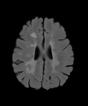
(a)

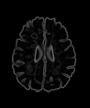
(b)

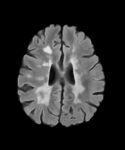
(c)

Figure 1: Intermediate image generation. (a) FLAIR image, (b) Sobel image, (c) intermediate image.

2.4 Hyperintensity probability map

The hyperintensity probability map is calculated based on the intermediate image generated during the pre-processing stage detailed in Section 2.3. We devised an algorithm that automatically generates such map and does not depend on parameters that must be set by experimental observations, as opposed to [16, 15].

The central principle behind this map is to compare each voxel neighborhood intensity with patches across different points in the image. The more times the voxel’s neighborhood mean intensity is higher than the patches’, then the more likely it is for that particular voxel to stand out and more likely for it to have a high hyperintense probability.

The first step to create the map is to define where each patch will be centered. To do that, we define a point net for each slice following the algorithm proposed in [15], which uses the combination of sines and cosines to evenly distribute points across a slice. Let $p=\{x,y,z\}$ be the coordinates of a candidate point. We then create new points $p^{\prime}=\{x^{\prime},y^{\prime},z\}$ with

$$\begin{array}[]{cc}x^{\prime}=&x+r\cos\theta\\ y^{\prime}=&y+r\sin\theta\end{array},$$ (6)

where $\theta$ is the angle and $r=10$ is the radius. We set $\theta$ to zero and increase it by 60 degrees six times to complete a whole circumference. The six newly defined points become candidate points, and the process repeats itself until no new point is found.

After defining such points, we prune the net using a brain mask to only keep points that are inside our ROI. This procedure is done by simply purging points outside the brain mask. An example of a final point net set $P$ for a particular slice is shown in Figure 2.

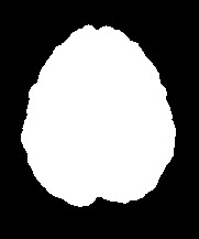
(a)

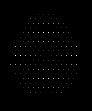
(b)

Figure 2: Brain mask (a) and pruned point net (b). Each patch of this particular slice is centered around one point in (b).

Now, let $\mu$ and $\sigma$ be the mean and standard deviation of the whole intermediate image within the brain mask. Then, for each voxel, we calculate its neighborhood mean intensity as

$$\mu_{v}=\frac{1}{N_{v}}\sum_{k=1}^{N_{v}}i_{k},$$ (7)

where $\mu_{v}$ is the mean neighborhood intensity of voxel $v$, $N_{v}$ is the number of neighbors of $v$ and $i_{k}$ is the intensity of neighbor $k$. The neighborhood size was defined as $3\times 3\times 3$ in order to maintain a good trade-off between sharpness and smoothness. The same rationale is used for the patches: the mean intensity is calculated as in Equation 7, thus creating $\mu_{p}$ for each patch.

Finally, we create a score $S_{v}$ as

$$S_{v}=\frac{1}{|P|}\sum_{p\in P}\delta(\mu_{v},\mu_{p}),$$ (8)

where $|P|$ is the cardinality of the patch set and

$$\delta(\mu_{v},\mu_{p})=\begin{cases}1,&\text{if }\mu_{v}-\mu_{p}\geq\sigma\\ 0,&\text{otherwise}\end{cases}.$$ (9)

In other words, if the difference of intensity between a candidate voxel neighborhood and a patch is greater than or equal to the standard deviation of the whole image, then it is a hit. Otherwise, it is a miss. By doing so, voxels with bright neighborhoods are enhanced while other regions and tissues are dimmed out. Moreover, since we normalize the score $S_{v}$, each voxel remains in the range $[0,1]$, which also serves as a hyperintensity probability indicator. An example of the map is shown in Figure 3.

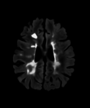
(a)

(b)

(c)

Figure 3: Hyperintensity map (a) compared to the original FLAIR image (b) and the intermediate image (c).

It is important to note that our approach does not require a hard threshold for Equation 9 or a fixed number of patches as it happens in [16]. Instead, the threshold is calculated automatically with respect to the standard deviation. Though simple, this is a significant improvement, since the main problem of using a hard threshold is that even normalized, intensities inherently vary from image to image. In this sense, a soft threshold such as the one we propose in this work may offer a better option for the enhancement of hyperintensities for it can adapt to each image intensity profile.

2.5 White matter mask estimation

The white matter region usually comprises most MS lesions [7]. An automatic brain segmentation into three clusters (WM, GM, and CSF) based on gray level intensities is most certainly going to mix lesions and cluster them as GM, WM or both [1, 21]. In this context, being able to estimate a mask that encompasses both white matter tissue and MS lesions may narrow down the ROI and increase the accuracy of lesion segmentation. To do so, we leveraged the fact that the map described in Section 2.4 can also be interpreted as a probability map and used it to get an estimate of such mask.

In this work, we made use of the Student t mixture model proposed in [11] and used T1-weighted and FLAIR images from each time-point to segment the brain into three different clusters and get an initial WM mask, herein referred to as $WM_{initial}$. To automatically identify the WM cluster from others, we used the WM probability map described in Section 2.1.2, averaged it over each cluster and selected the one with the highest WM probability.

Since the 2015 Longitudinal MS Lesion Segmentation Challenge did not provide WM ground truths, we created our own using a straightforward approach. Given any $WM_{initial}$, we simply merged it with the lesions ground truth to get the whole WM region in one single mask, herein referred to as $WM_{whole}$. Considering that each time-point had two different lesions ground truth, we created two WM masks for each time-point as well.

The actual WM estimation took place as follows. First, we calculated the mean ($\mu_{HI}$) and standard deviation ($\sigma_{HI}$) of the region defined by $WM_{initial}$ on the hyperintensity map image and the mean ($\mu_{prob}$) of the region defined by $WM_{initial}$ on the WM probability atlas. The idea was to expand $WM_{initial}$ by considering voxels that are not part of the mask yet and analyzing $3\times 3\times 3$ neighborhoods centered around these voxels to verify their potential for being included. The expansion itself occurred by incorporating voxels that seemed as outliers; more precisely, voxels with mean neighborhood values greater than $\mu_{HI}+1\times\sigma_{HI}$ in the hyperintensity map and greater than $\mu_{prob}$ in the probability atlas. A pseudo-algorithm for estimating the white matter mask is presented in Algorithm 1 and an example of the output of this estimation is shown in Figure 4.

Input: $\text{WM}_{initial}$, $\text{HI}_{map}$, $\text{WM}_{prob}$

Output: $\text{WM}_{estim}$

1:$i\leftarrow 3$

2:$WM_{estim}\leftarrow WM_{initial}$

3:$\mu_{HI},\sigma_{HI}\leftarrow MeanAndSigma(WM_{estim},HI_{map})$

4:$\mu_{prob}\leftarrow Mean(WM_{estim},WM_{prob})$

5:$t_{prob}\leftarrow\mu_{prob}$

6:$t_{HI}\leftarrow\mu_{HI}+i\times\sigma_{HI}$

7:for each voxel not in $WM_{estim}$ do

8:     $WM_{estim}\leftarrow ExpandWM(WM_{estim},HI_{map},WM_{prob},t_{HI},t_{prob})$

9:end for

Algorithm 1 White matter mask estimation algorithm

(a)

(b)

(c)

(d)

Figure 4: White matter estimation output. (a) Hyperintensity map, (b) $WM_{initial}$, (c) $WM_{ground\,truth}$ and (d) $WM_{estim}$.

2.6 Pure white matter and gray matter clusters

To estimate the intensity profiles of white matter and gray matter clusters without lesions, we did the following. For each time-point segmentation, we automatically identified the white and gray matter clusters by analyzing their mean intensities on white and gray matter probabilistic atlases. The cluster with highest white matter atlas mean intensity was taken as the white matter cluster ($WM_{initial}$); the same rationale was used for the gray matter cluster ($GM_{initial}$). Then, for each expert annotation, we simply excluded every voxel that had any intersection with the lesion ground truth and these two clusters. Formally, $WM_{pure}=WM_{initial}-(WM_{initial}\cap GT_{E\in\{\text{Expert 1, Expert 2}\}})$ and $GM_{pure}=GM_{initial}-(GM_{initial}\cap GT_{E\in\{\text{Expert 1, Expert 2}\}})$. By doing so, we were able to get so-called “pure” WM and GM clusters, which were then used to calculate their intensity profiles and compare them to lesion profiles in Section 3.1.

3 Results

In this section, we present the results regarding the brightness intensity profile of MS lesions compared to gray matter and white matter on FLAIR, intermediate and hyperintensity map images for each patient.

For the sake of comparison, all images were rescaled to the range $[0,1]$ and the results in Section 3.1 are shown in percentage; that is, how much brighter, percent-wise, the lesion profile was compared to other brain tissues.

We also present the Dice and lesion intersection metrics regarding the white matter mask in Section 3.2 to offer a quantitative analysis of the mask estimation.

It is important to remember that each patient had a number of time-points made available. For the sake of understandability and inter-patient comparison, every result presented in Sections 3.1 and 3.2 represents the average of all time-points of a particular patient.

3.1 Brightness profile

Since the 2015 Longitudinal MS Lesion Segmentation Challenge provided two ground truths for each time-point, we extracted the intensity profiles for both annotations. We rescaled all images to the $[0,1]$ interval, averaged the white matter, gray matter and lesion profiles and also calculated the standard deviation for each patient. The results are shown in Figures 5 and 6 for experts 1 and 2, respectively.

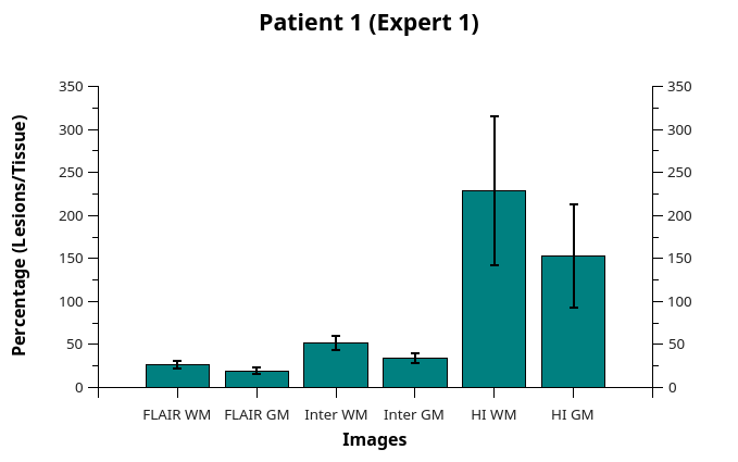
(a)

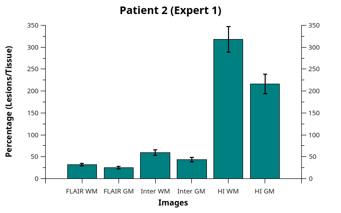
(b)

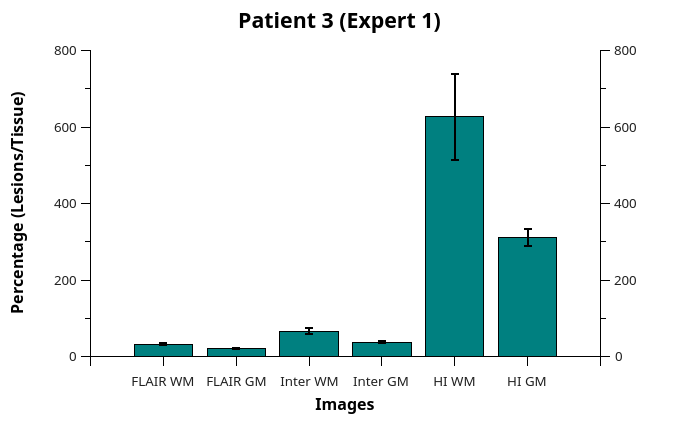
(c)

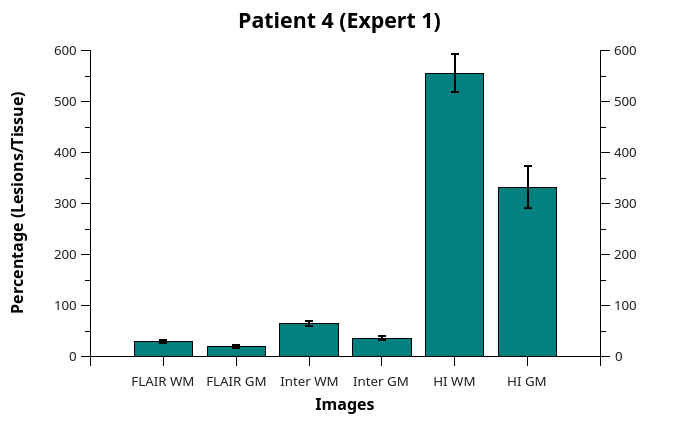
(d)

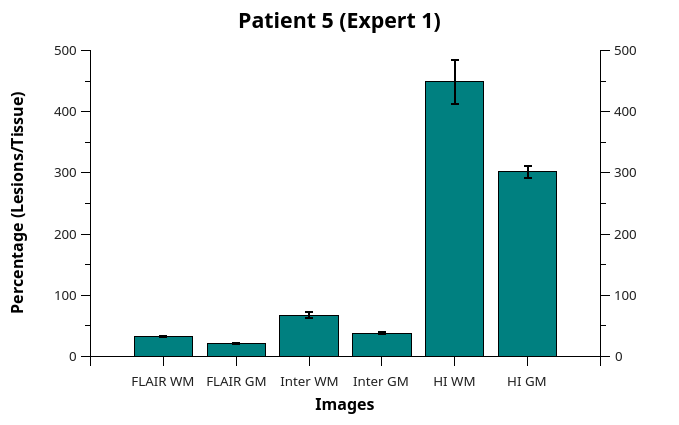
(e)

Figure 5: Lesion intensity profile compared to white matter and gray matter tissues using ground truths from expert 1. Here, “Inter” is the intermediate image and “HI” is the hyperintensity map. Each bar represents the mean lesion intensity over the mean intensity of a given tissue (white matter or gray matter) in a particular image type.

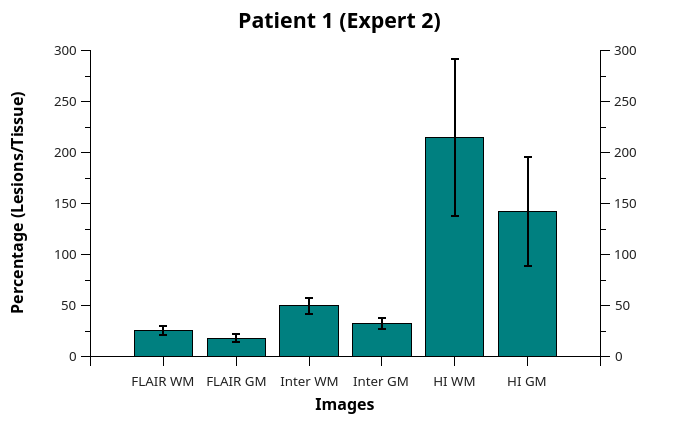
(a)

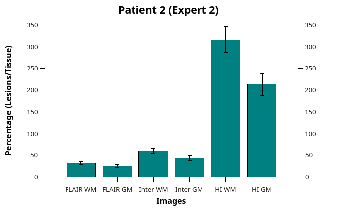
(b)

(c)

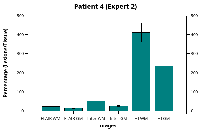
(d)

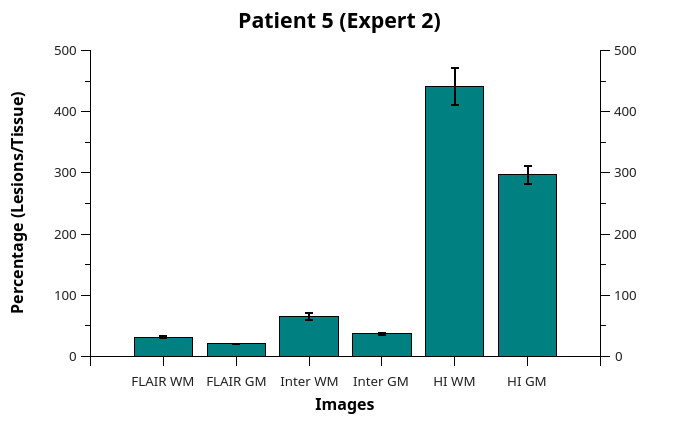
(e)

Figure 6: Lesion intensity profile compared to white matter and gray matter tissues using ground truths from expert 2. Here, “Inter” is the intermediate image and “HI” is the hyperintensity map. Each bar represents the mean lesion intensity over the mean intensity of a given tissue (white matter or gray matter) in a particular image type.

Each bar in Figures 5 and 6 represents the mean lesion intensity over the mean intensity of a given tissue (gray matter or white matter) in a particular image type (FLAIR, intermediate and hyperintensity map). For instance, the FLAIR WM bar in Figure 5(a) must be interpreted as “the average MS lesion profile in FLAIR images from Patient 1 is approximately 25% brighter than the average WM tissue intensity for the same image type and patient”. This result allows a direct comparison between tissues and images.

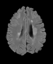
(a)

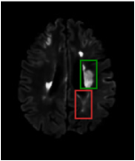
(b)

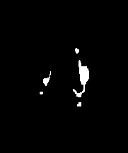
(c)

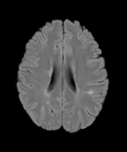
(d)

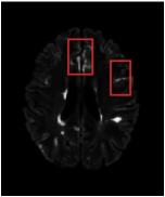
(e)

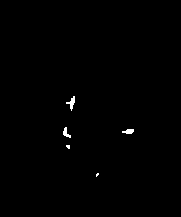
(f)

Figure 7: Intensity problems caused by wide lesion intensity range (first row) and hyperintensities in regions other than lesions (second row).

3.2 White matter mask comparison

We compared the white matter mask estimated in Section 2.5 with our WM ground truths using the Dice coefficient. We also extracted the percentage of lesions (intersection) present in each estimated mask to analyze the lesion load that was kept during the estimation. Again, since there were two lesion ground truths for each time-point, we extracted metrics for both experts. The results are presented in Table 2 and shown in Figures 8 and 9.

	LI (%) Expert 1 ($\mu\pm\sigma$)	LI (%) Expert 2 ($\mu\pm\sigma$)	Dice Expert 1 ($\mu\pm\sigma$)	Dice Expert 2 ($\mu\pm\sigma$)
Patient 1	78.56 $\pm$ 6.7	77.65 $\pm$ 8.30	0.9763 $\pm$ 0.0003	0.9764 $\pm$ 0.0007
Patient 2	89.60 $\pm$ 1.59	88.20 $\pm$ 1.71	0.9786 $\pm$ 0.0021	0.9775 $\pm$ 0.0020
Patient 3	83.88 $\pm$ 0.94	79.08 $\pm$ 2.51	0.9834 $\pm$ 0.0007	0.9829 $\pm$ 0.0005
Patient 4	76.83 $\pm$ 1.20	56.95 $\pm$ 4.03	0.9860 $\pm$ 0.0012	0.9853 $\pm$ 0.0013
Patient 5	73.73 $\pm$ 3.55	71.00 $\pm$ 2.16	0.9828 $\pm$ 0.0017	0.9826 $\pm$ 0.0017

Table 2: Lesion intersection (LI) and Dice coefficients for the white matter mask estimation for both expert ground truths.

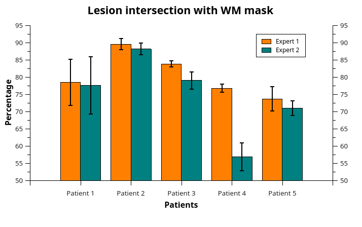
Figure 8: Lesion intersection with the estimated white matter mask using ground truths from both experts.

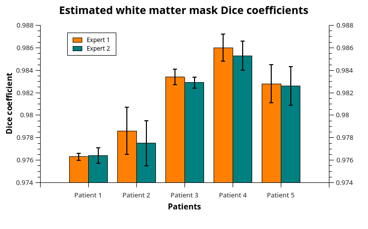
Figure 9: Dice coefficients of the estimated white matter mask compared to ground truths created using experts lesion annotations and automatic brain segmentation.

4 Discussion

The results in Figures 5 and 6 indicate a significant difference in the MS lesion intensity profile in the hyperintensity map compared to FLAIR and the intermediate image described in Section 2.3. This result is a significant outcome, because it provides quantitative background to show the discriminative features of the HI map.

It is possible to note that the lesion intensity profile was more similar to gray matter than to white matter. The difference in intensity between MS lesions and these two tissues in FLAIR and intermediate images was minimal compared to the HI map, which showed, in the worst case (Patient 1, Expert 2, GM), a 141% brightness gap. In contrast, this same case presented an 18% and 32% IPD for FLAIR and intermediate images.

At the same time, the standard deviation in the HI map was far bigger than in FLAIR and intermediate images, which is an indicator that the map has a rather spread out MS lesion intensity profile. While this is a concern that must be addressed when using the map to segment lesions, whether manually or automatically, the overall difference in intensity between lesions and other brain tissues is still significant and may provide enough leverage to overcome, at least partially, the wide standard deviation variation.

Moreover, a distinct drawback of the HI map is that it is highly dependent on the gray level intensity in FLAIR. This fact poses two problems that can be seen in Figure 7. The first one is presented in Figure 7(a)-(c) and concerns the natural intensity variation within the lesion profile. In this case, the lesion enclosed by the red rectangle was not as enhanced as the one enclosed by the green rectangle. As seen in Figure 7(a), the red rectangle lesion did not present a profile as hyperintense as the green one in FLAIR, so this difference was propagated to the HI map. The other problem is shown in Figure 7(d)-(f). Areas enclosed by red rectangles indicate regions that do not have MS lesions and yet are enhanced in the map. Again, this happens because these regions presented rather high-intensity profiles in FLAIR and thus were enhanced in the map. Both these problems may interfere with lesion segmentation accuracy and indicate that the HI map should not be used as a stand-alone feature in manual and automatic segmentation techniques.

While there are some works in the literature [17, 19, 1] that mention MS lesion intensity profiles and how they relate to other tissues, none of them provide a quantitative analysis regarding percentage, making it difficult to to compare our results with theirs objectively. The databases are also different. However, analyzing scatter plots in [17, 19], it is possible to see that lesion intensity profiles present a significant overlap with other brain tissues. Hence, the HI map can undoubtedly help distinguish lesions more easily.

On the white matter mask estimation, the results are shown in Table 2 and in Figures 8 and 9 indicate high DSCs and a significant intersection with lesions. A relevant observation to be made is that the LI metric presented a consistent level of intersection regardless of lesion volumes, which is an indication of robustness.

In Figure 8, it is possible to note that patient 4 presented very different results on lesion intersection. The reason for this is that the expert annotations for this patient had the smallest DSC ($0.612\pm 0.0019$) among all patients, as mentioned in [11]. In other words, experts did not have a high agreement coefficient on lesion segmentation for this particular case, which consequently made our technique present very different intersection values for each annotation.

Another point to be made about Figure 8 is that patient 1 presented the biggest standard deviation of all. This result came from the fact that this patient’s lesion intensities faded across time-points, making the enhancement less effective. This fading phenomenon can also be seen in Figures 5 and 6, since patient 1 had the biggest standard deviation on the lesion intensity profile in the HI map compared to other patients.

As mentioned in Section 1, there are various works in the literature focused on automatic brain tissue segmentation [1, 21, 22, 23]. Though a direct comparison is not possible due to different metrics being used and database access restrictions, the closest work to ours regarding white matter estimation was [23]. Contrary to the authors approach, our proposal requires only FLAIR images (from which the HI maps are created) and WM probability atlases to fill lesion holes left out during an automatic segmentation process. It is important to note that our technique focuses only on the white matter region at this point, while all three major brain tissues are segmented in [23]. However, we believe that it is possible to extend our work to also handle gray matter and cerebrospinal fluid tissues, thus allowing a thorough comparison between techniques in the future.

5 Conclusions

This work presented an automatic technique based on the works of [16, 15] to enhance hyperintensities in FLAIR images, making it easier to distinguish multiple sclerosis lesions from other brain tissues, namely gray matter and white matter. By defining a metric called Intensity Profile Difference (IPD), we were able to analyze, percent-wise, how much brighter the lesion profile was compared to other tissues and image types on five patients from the 2015 Longitudinal Multiple Sclerosis Lesion Segmentation Challenge.

The hyperintensity map, created by the enhancement process, offered a much more distinct lesion profile compared to FLAIR. On average, lesions presented a mean intensity profile 444.57% and 264.88% brighter than white matter and gray matter in the HI map, respectively. In FLAIR, the same profile was only 25% and 19% brighter considering the same tissues. This result may serve as an essential aid for both manual and automatic segmentation techniques.

The HI map is heavily based on gray level intensities and has two drawbacks worth of notice. The first one regards the intensity variation within lesions since the difference in intensity from one lesion to another in FLAIR is propagated to the map. The second drawback regards regions that do not have lesions but also appear hyperintense in FLAIR. These regions are also enhanced in the map, which may lead to false positives. Due to this reason, the HI map should not be used as a stand-alone feature in applications such as tissue or lesion segmentation.

A byproduct of the HI map is an initial estimate of the white matter mask for a given time-point. Automatically segmenting a brain image with multiple sclerosis into three clusters (white matter, gray matter, and cerebral spinal fluid) will undoubtedly mix lesions with other tissues. In this sense, we can simply get the white matter cluster mask and fill regions that are not yet in the mask but are above a certain threshold in the map to get a “full” WM mask. The estimation of the white matter area may be relevant to narrow down the ROI when segmenting lesions and also help with brain tissue segmentation and volume assessment.

We showed that lesions have an intensity profile that is brighter than white matter than it is to gray matter, so we believe that restricting the segmentation area to a mask that excludes most gray matter region might increase lesion segmentation accuracy. However, the two problems mentioned before about the HI map also affected the white matter mask estimation. Part of the lesions was left out, as evidenced by the LI metric, and some regions not related to white matter were included in the estimation.

In conclusion, the results of this study showed that the hyperintensity map offers a much more distinct profile for multiple sclerosis lesions compared to white matter and gray matter tissues in FLAIR and such map can also be used to estimate an initial white matter mask. In future works, we aim to address the problems with the enhancement algorithm mentioned earlier and efficiently use it to increase both tissue and lesion segmentation accuracies in automatic techniques. We also plan on extending the white matter estimation technique to the other two primary brain tissues (white matter and cerebrospinal fluid).

References

- [1] M. Battaglini, M. Jenkinson, and N.D. Stefano. Evaluating and reducing the impact of white matter lesions on brain volume measurements. Human Brain Mapping, 33(9):2062–2071, 2012.
- [2] P. Browne, D. Chandraratna, C. Angood, H. Tremlett, C. Baker, B. Taylor, and A. Thompson. Atlas of multiple sclerosis 2013: A growing global problem with widespread inequity. Neurology, 83(11):1022, 1024 2013.
- [3] A. Buades, B. Coll, and J-M. Morel. A non-local algorithm for image denoising. IEEE Computer Society Conference on Computer Vision and Pattern Recognition, 2:60–65, 2005.
- [4] A. Carass, J. Cuzzocreo, M.B. Wheeler, P.-L. Bazin, S.M. Resnick, and J. Prince. Simple paradigm for extra-cerebral tissue removal: Algorithm and analysis. NeuroImage, 56(4):1982–1992, 2011.
- [5] A. Carass, S. Roy, A. Jog, J.L. Cuzzocreo, E. Magrath, A. Gherman, J. Button, J Nguyen, F. Prados, C.H. Sudre, M. Jorge Cardoso, N. Cawley, O. Ciccarelli, C.A. Wheeler-Kingshott, Ourselin S., L. Catanese, H. Deshpande, P. Maurel, O. Commowick, C. Barillot, X. Tomas-Fernandez, S.K. Warfield, S. Vaidya, A. Chunduru, R. Muthuganapathy, G. Krishnamurthi, A. Jesson, T. Arbel, O. Maier, H. Handels, L.O. Iheme, D. Unay, S. Jain, D.M. Sima, D. Smeets, M. Ghafoorian, B. Platel, A. Birenbaum, H. Greenspan, P.L. Bazin, P.A. Calabresi, C.M. Crainiceanu, L.M. Ellingsen, D.S. Reich, J.L. Prince, and D.L. Pham. Longitudinal multiple sclerosis lesion segmentation: Resource and challenge. NeuroImage, 148:77–102, 2017.
- [6] A. Carass, M.B. Wheeler, J. Cuzzocreo, P.-L. Bazin, S.S. Bassett, and J. Prince. A Joint Registration and Segmentation Approach to Skull Stripping. In Proceedings of the 4th IEEE International Symposium on Biomedical Imaging: From Nano to Macro, pages 656–659, Arlington, VA, USA, April 2007. IEEE.
- [7] A. Compston and A. Coles. Multiple Sclerosis. Lancet, 372(9648):1502–1517, October 2008.
- [8] L.R. Dice. Measures of the amount of ecologic association between species. Ecology, 26(3):297–302, 1945.
- [9] O.R. Duda, P.E. Hart, and D.G. Stork. Pattern Classification (2Nd Edition). Wiley-Interscience, Hoboken, USA, 2000.
- [10] V.S. Fonov, A.C. Evans, R.C. McKinstry, Almli C.R., and D.L. Collins. Unbiased nonlinear average age-appropriate brain templates from birth to adulthood. NeuroImage, 47:S102, 2009.
- [11] P.G.L. Freire and R.J. Ferrari. Automatic iterative segmentation of multiple sclerosis lesions using Student’s t mixture models and probabilistic anatomical atlases in FLAIR images. Computers in Biology and Medicine, 73:10–23, 2016.
- [12] R.H. Hashemi, W.G. Bradley, Y.D. Chen, J.E. Jordan, J.A. Queralt, A.E. Cheng, and J.N. Henrie. Suspected mutiple sclerosis: MR imaging with a thin-section fast FLAIR pulse sequence. Radiology, 196(2):505–510, 1995.
- [13] M. Modat, G.R. Ridgway, Z.A. Taylor, M. Lehman, J. Barnes, D.J. Hawkes, N.C. Fox, and S. Ourselin. Fast free-form deformation using graphics processing units. Computer Methods and Programs in Biomedicine, 98(3):278–284, 2010.
- [14] L. Nyúl, J. Udupa, and X. Zhang. New Variants of a Method of MRI Scale Normalization. IEEE Transactions on Medical Imaging, 19(2):143–150, 2000.
- [15] P.K. Roy, A. Bhuiyan, A. Janke, P.M. Desmond, T.Y. Wong, E. Storey, W.P. Abhayaratna, and K. Ramamohanarao. Automated segmentation of white matter lesions using global neighbourhood given contrast feature-based random forest and Markov random field. In Proceedings of the 2014 IEEE International Conference on Healthcare Informatics, pages 1–6, Verona, Italy, September 2014. IEEE.
- [16] P.K. Roy, A. Bhuiyan, and K. Ramamohanarao. Automated Segmentation of multiple sclerosis lesion in intensity enhanced FLAIR MRI using texture features and support vector machine. In Proceedings of the 20th IEEE International Conference on Image Processing, pages 4277–4281, Melbourne, VIC, Australia, September 2013. IEEE.
- [17] M. Shah, Y. Xiao, N. Subbanna, S. Francis, D. Arnold, D. Collins, and T. Arbel. Evaluating intensity normalization on MRIs of human brain with multiple sclerosis. Medical Image Analysis, 15:267–282, 2011.
- [18] N. Shiee, P.-L. Bazin, J.L. Cuzzocreo, C. Ye, B. Kishore, A. Carass, P.A. Calabresi, D.S. Reich, J.L. Prince, and D. Pham. Robust Reconstruction of the Human Brain Cortex in the Presence of the WM Lesions: Method and Validation. Human Brain Mapping, 35(7):3385–3401, 2014.
- [19] X. Tomas-Fernandez and S. Warfield. A model of population and subject (MOPS) intensities with application to multiple sclerosis lesion segmentation. IEEE Transactions on Medical Imaging, 34(6):1349–1361, 2015.
- [20] N. Tustison and J. Gee. N4ITK: Nick’s N3 ITK implementation for MRI bias field correction. Penn Image Computing and Science Laboratory, 2009.
- [21] S. Valverde, O.A. Dez, Y. Cabezas, M. Vilanova, J. Rami-Torrentà, A. Rovira, and X. Lladó. Evaluating the effects of white matter multiple sclerosis lesions on the volume estimation of 6 brain tissue segmentation methods. American Journal of Neuroradiology, 36(6):1109–1115, 2015.
- [22] S. Valverde, A. Oliver, M. Cabezas, E. Roura, and Lladó X. Comparison of 10 brain tissue segmentation methods using revisited IBSR annotations. Journal of Magnetic Resonance Imaging, 41:93–101, 2015.
- [23] S. Valverde, A. Oliver, E. Roura, S. González-Villà, D. Pareto, J. Vilanova, L. Ramío-Torrentà, A. Rovira, and X. Lladó. Automated tissue segmentation of MR brain images in the presence of white matter lesions. Medical Image Analysis, 35:446–457, 2016.
- [24] S. Warren and K. Warren. Mutiple sclerosis. http://bit.ly/2AbSVqj, 2001. Last accessed in November 28th, 2017.
- [25] World Health Organization. Atlas - multiple sclerosis resources in the world. http://bit.ly/14Ddglh, 2008. Last accessed in November 28th, 2017.