Jellium and Cell Model for Titratable Colloids with Continuous Size Distribution

Abstract

A good understanding and determination of colloidal interactions is paramount to comprehend and model the thermodynamic and structural properties of colloidal suspensions. In concentrated aqueous suspensions of colloids with a titratable surface charge, this determination is, however, complicated by the density dependence of the effective pair potential due to both the many-body interactions and the charge regulation of the colloids. In addition, colloids generally present a size distribution which results in a virtually infinite combination of colloid pairs. In this paper we develop two methods and describe the corresponding algorithms to solve this problem for arbitrary size distributions. An implementation in Nim is also provided. The methods, inspired by the seminal work of Torres et al., are based on a generalization of the cell and renormalized jellium models to polydisperse suspensions of spherical colloids with a charge regulating boundary condition. The latter is described by the one-pK-Stern model. The predictions of the models are confronted to the equations of state of various commercially available silica dispersions. The renormalized Yukawa parameters (effective charges and screening lengths) are also calculated. The importance of size and charge polydispersity as well as the validity of these two models are discussed in light of the results.

I Introduction

Size polydispersity, rather than being an exception, is a general rule in the realm of colloidal systems. It has been shown to influence the micro structure of suspensions D’Aguanno and Klein (1991), to considerably enrich the number of crystal phases observed Shevchenko et al. (2006); Evers et al. (2010); Cabane et al. (2016); Schaertl, Palberg, and Bartsch (2017), to affect nucleationAuer and Frenkel (rint); van der Linden, van Blaaderen, and Dijkstra (2013); Palberg, Wette, and Herlach (2016), to induce the fractionation of particles during crystallizationDijkstra, Frenkel, and Hansen (1994); Bolhuis and Kofke (1996); Kofke and Bolhuis (1999); Byelov et al. (2010); Cabane et al. (2016) and to allow particular behavior such as colloidal Brazil nut effect Esztermann and Löwen (2004); Noguera-Marín et al. (2015), colloidal stratification Fortini et al. (2016); Zhou, Jiang, and Doi (2017) and fluid-fluid demixingAarts (2005); Dijkstra, van Roij, and Evans (1998); Zvyagolskaya, Archer, and Bechinger (2011). Moreover, polydispersity has been shown to be an essential feature in the formation of colloidal glassesPusey and van Megen (1986); Barrat and Hansen (1986) and has allowed substantial achievements in the understanding of this state, see e.g. Refs Fernández, Mart$\backslash$’ın-Mayor, and Verrocchio, 2007; Pusey et al., 2009; Palberg et al., 2016; Berthier et al., 2017.

Despite its ubiquity, polydispersity is still often neglected, with the exception of neutral hard sphere systems, and the variety of phases, states and behaviors that it brings about are imperfectly controlled and understood. The main reason for this is the fact that computer simulations still lag well behind experimental observations, when appropriate models exist at all. This is particularly true for charged colloidal suspensions, the system of interest in this paper.

From a simulation point of view, representative and realistic models of charged polydisperse colloidal suspensions are indeed tractable neither at the primitive model level of approximation, where the degrees of freedom of the solvent molecules are averaged out through a dielectric continuum, nor at the level of the mean field approximationFushiki (1992); Dobnikar et al. (2003); Hallez, Diatta, and Meireles (2014), where the many ions are further replaced by a mean electrostatic potential obtained from solving the Poisson-Boltzmann equation. An amenable and attractive approach, first introduced by Beresford-Smith Beresford-Smith, Chan, and Mitchell (1985), consists, instead, in whittling the colloidal system down to the colloidal particles only, i.e. the one-component model, while the degrees of freedom of the ions and solvent molecules are integrated out in effective pair potentials between the colloids, $w^{\ast}(r)$. The reduction of the many-body interactions into effective potentials, however, makes $w^{\ast}$ density dependent Brunner et al. (2002) and, thus, necessarily re-determined for each colloid density.

In the case of monodisperse spherical particles at low electrostatic coupling, Alexander et al. Alexander et al. (1984) showed that $w^{\ast}(r)$ retains a simple Yukawa form but with effective parameters, namely an effective charge, $Z^{\ast}$, and screening length, $1/\kappa^{\ast}$, instead of the bare charge, $Z$ and bulk screening length, $1/\kappa$. The study further showed that $Z^{\ast}$ and $\kappa^{\ast}$ can be obtained from solving the Poisson-Boltzmann equation around one colloid placed in Wigner-Seitz cell model (CM)Marcus (1955). In the same spirit, a one-colloid renormalized jellium model was developed and shown to be successful in salt free systems Trizac and Levin (2004). At high electrostatic coupling, two-colloids cell Turesson, Jönsson, and Labbez (2012) and jellium models Bareigts and Labbez (2017) solved in the full primitive model were shown to provide accurate $w^{\ast}(r)$ for arbitrary colloid shapes Thuresson, Ullner, and Turesson (2014) and concentrations. The two-colloid approach was further used at a molecular level Bonnaud et al. (2016) in a 3D-periodic simulation box.

In the case of charged colloid mixtures, Torres et al. Torres, Téllez, and van Roij (2008) proposed a generalization of the cell model. The great insight of Torres and co-workers was simply to impose the same potential at the boundary of each cell, each family of colloidal particles being represented by one colloidal particle of the same radius centered in its own Wigner-Sietz cell, in such a way as to ensure the continuity of electric potential and ion concentrations across the cell boundaries. The greatest ideas also being the simplest, it was then followed to generalize the jellium model Falcón-González and Castañeda-Priego (2011); García de Soria, Álvarez, and Trizac (2016). However, to our knowledge the generalized cell and jellium models have only been tested in the salt free case García de Soria, Álvarez, and Trizac (2016). Furthermore, they have so far always been restricted to binary mixtures, i.e. have never been applied to polydisperse charged colloidal suspensions with continuous size distribution.

Another difficulty arises from the nature of the surface charge and its dependence on the density and size polydispersity of colloidal suspensions, namely the charge regulation and the charge polydispersity. Both largely depend on the chemistry of the colloid surface and of the electrolyte but also on the surface curvature and strength of the interactions and are, thus, specific to each colloidal system. The aqueous surface chemistry and charging behavior of colloidal particles has been the subject of many investigations essentially concerning the thermodynamic limit of infinite (colloid) dilution, see e.g. Refs. Hunter, 1995; Hiemstra and Van Riemsdijk, 1996; Borkovec, 1997; Lyklema, 2005. On the contrary, in studies of the structure of colloidal suspensions, the charging behavior (of colloids) is most often simply ignored the assumption being a constant surface density or at best a constant electrical double layer potential Smallenburg et al. (2011). This can be explained in part by the complexity of characterization and, thus, by the poor knowledge of the charging behavior of colloids in non diluted suspensions, not to mention the charge polydispersity, as indicated by the very limited research work available Wette, Schöpe, and Palberg (2002); Lobaskin et al. (2007); Merrill, Sainis, and Dufresne (2009). Very rarely have attempts been made to include a description of surface chemistry Gisler et al. (1994); von Grünberg (1999); Heinen, Palberg, and Löwen (2014). Furthermore, those that do exist are, again, all limited to monodisperse systems.

Motivated by the recent experimental results obtained by Cabane et al.Cabane et al. (2016) on aqueous suspensions of titrating silica nanoparticles with large polydispersity, which show a fractionation of particles in three coexisting phases (Laves/BCC/liquid phases) in the semi-concentrated regime and high pH, we here develop two methods and describe the corresponding algorithms to estimate the charging behavior and charge polydispersity of titrating silica particles with a continuous size distribution. The methods are further used to evaluate the sets of effective parameters (i.e. $Z^{\ast}$ and $\kappa^{\ast}$) to be used in a one-component model. The methods, largely inspired by the seminal work of Torres et al.Torres, Téllez, and van Roij (2008), are based on a generalization of the cell and renormalized jellium models to polydisperse suspensions of spherical colloids supplemented with a charge regulating boundary condition described by a 1-p$K$-Stern model. Certain features are studied, in particular, the dependence of the charge polydispersity as well as its scaling with the surface curvature on the size polydispersity and density of the colloids. Finally, the validity of the proposed models is discussed in terms of their ability to describe the equation of state of various commercially available silica dispersions.

The manuscript is organized as follows: in Sect. II we introduce the models used, that is, in Sect. II.1 and II.2, the generalized cell model and jellium model for charged polydisperse colloidal suspensions and, in Sect. II.3, the 1-pK Stern model to describe the interface between the solid and the electrolyte solution in the presence of acidic surface groups. In Sect. II.4 the algorithm used to solve the cell and jellium models coupled with the 1-pK Stern model is described. In Sect. III.1 we present the 1-p$K$-Stern model fit of the charging behavior of silica surfaces in the dilute regime together with the CM and RJM predictions of the bare charge polydispersity of silica nanoparticles with various polydispersities and densities, and in various pH conditions. The corresponding effective charge polydispersities and effective screening lengths are presented in Sect. III.2. Microion pressures for various polydispersities and distribution shapes is studied in Sect III.3. Finally, experimental data are compared with the predictions of the cell and jellium model in the same section, followed by conclusions in Sect. IV.

II Models

Let us consider a polydisperse colloidal suspension composed of $n_{p}$ spherical colloidal species of radii $R_{p}$ bearing a charge $Q_{p}=Z_{p}e$ with $e$ the elementary charge and $p=1,\dots,n_{p}$. They are immersed in a volume $V$ filled with an aqueous salt solution of dielectric constant $\epsilon$ in equilibrium with a reservoir at a temperature $T$ and of inverse screening length,

$$\kappa=\sqrt{4\pi\lambda_{B}\sum_{i=1}^{n_{i}}z_{i}^{2}c_{s,i}},$$ (1)

where $\lambda_{B}=\frac{e^{2}}{4\pi k_{B}T\epsilon}$ is the Bjerrum length and $k_{B}$ is the Boltzmann constant while $z_{i}$ and $c_{s,i}$ are the number valence and bulk concentration of ionic species $i$, respectively. $n_{i}$ is the total number of ion species. The composition of each colloidal species is defined by its number fraction $x_{p}=N_{p}/\sum_{n_{p}}N_{p}$.

Within the mean-field approximation of the primitive model, the electrostatic potential at the surface of the colloids, at a set configuration of the latter, and in the electrolyte solution is determined by solving the Poisson-Boltzmann equation, which for an arbitrary system is given byIsraelachvili (1991)

$$\epsilon\bigtriangleup V(\vec{r})+\sum_{i=1}^{n_{i}}z_{i}ec_{i}(\vec{r})+\rho_{e}(\vec{r})=0,$$ (2)

where $\vec{r}$ is the vector position in the solution, $V$ is the electrostatic potential, $\bigtriangleup$ is the Laplace operator, $c_{i}(\vec{r})=c_{s,i}\exp\left(\frac{-z_{i}eV(\vec{r})}{k_{B}T}\right)$ and $\rho_{e}$ is a charge density associated with the colloids, specified later according to the model.

Within the approximation of the polydisperse cell model (PCM) and polydisperse renormalized jellium model (PRJM) it is only necessary to solve Equation 2 with one colloid with the appropriate boundary conditions and to repeat it for each colloid species. Taking further advantage of the spherical symmetry, the electrostatic potential becomes a mere function of the radial coordinate $r$ and Eq. 2 reduces to

$$\frac{\partial^{2}\psi}{\partial r^{2}}+\frac{1}{r}\frac{\partial\psi}{\partial r}+4\pi\lambda_{B}\left[\sum_{i=1}^{n_{i}}z_{i}c_{s,i}\exp(-z_{i}\psi(r))+\xi(r)\right]=0,$$ (3)

where for convenience, we have introduced the dimensionless potential $\psi=\frac{eV}{k_{B}T}$ and the reduced charge density $\xi=\rho_{e}/e$. The surrounding colloids are effectively accounted for through the boundary conditions and $\xi$ which depends on the model used. They are detailed below.

II.1 Cell model

The cell model approximation emerged was initially designed for colloidal crystals and emerged from the realization that due to its periodicity the volume of a crystal can be divided into electroneutral Wigner-Seitz cells surrounding each colloid which on average have the same volume and contain the same ion concentrationsAlexander et al. (1984). In other words, the thermodynamic properties of the system can be reduced to one colloid enclosed in an appropriate cell. The geometry of the cell is further assumed to have the same shape as the colloid. A spherical cell of radius $R_{c}$ centered on the colloid is a natural choice for a spherical colloid. Note that the cell model approximation was also shown to be valid for non spherical colloids and moderately concentrated fluid statesReiner and Radke (1991); Löwen (1994); Bocquet, Trizac, and Aubouy (2002).

Within this approximation, $\xi=0$ and, thus, the PB equation, Eq. 3, within the electrolyte solution takes the usual form

$$\bigtriangleup\psi(r)=\kappa^{2}\sinh\psi(r)\text{ with }R_{p}<r<R_{c}.$$ (4)

Note that here a 1-1 salt solution is considered. The Gauss law imposes that the electric field be null everywhere on the boundary of the electroneutral cell,

$$\frac{\partial\psi}{\partial r}\Big{|}_{r=R_{c}}=0.$$ (5)

The missing boundary condition at the colloid surface is described below (Sect. II.3).

For monodisperse dispersions the cell radius is commensurate with the particle volume fraction $\Phi$,

$$\Phi=\left(\frac{R}{R_{c}}\right)^{3}.$$ (6)

Similarly, for polydisperse dispersions, the cell radii of the colloidal species, $R_{c,p}$, are related to the overall particle volume fraction by

$$\Phi=\frac{\sum_{p=1}^{n_{p}}x_{p}R_{p}}{\sum_{p=1}^{n_{p}}x_{p}R_{c,p}^{3}}.$$ (7)

These unknown variables are determined by imposing the continuity of the electrical potential and ion concentrations over the different cellsTorres, Téllez, and van Roij (2008). That is to say,

$$\psi(R_{c,1})=\psi(R_{c,2})=\dots=\psi(R_{c,n_{p}})=\psi_{c}.$$ (8)

In the case of suspensions of colloids immersed in mono-monovalent salt solutions, the effective pair potential between the colloids keeps the form of a screened Coulomb potential,

$$\beta u(r_{pq})=\lambda_{B}\upsilon_{p}Z^{\ast}_{p}\upsilon_{q}Z^{\ast}_{q}\frac{\exp({-\kappa^{\ast}r})}{r},$$ (9)

but with the renormalized charges and inverse screening length as leading parameters. In the previous equation $\upsilon_{p}=\exp(\kappa^{\ast}R_{p})/(1+\kappa^{\ast}R_{p})$ ensures that the ionic cloud is excluded from the core of the colloid. Following the elegant method of Trizac et al.Trizac et al. (2003) those renormalized parameters can be obtained analytically from the calculated electrostatic potential at the edge of the cell. That is,

$$\kappa^{\ast}=\sqrt{4\pi\lambda_{B}\sum_{i=1}^{n_{i}}z_{i}^{2}c_{s,i}\exp(-z_{i}\psi_{c})}$$ (10)

and

$$Z^{\ast}_{p} =\frac{\gamma_{0}}{\kappa^{\ast}\lambda_{B}}\left[((\kappa^{\ast})^{2}R_{c,p}R_{p}-1)\sinh\kappa^{\ast}(R_{c,p}-R_{p})\right.$$

$$\left.+(\kappa^{\ast})^{2}+\kappa^{\ast}(R_{c,p}-R_{p})\sinh\kappa^{\ast}(R_{c,p}-R_{p})\right],$$ (11)

where

$$\gamma_{0}=\frac{-4\pi\lambda_{B}}{(\kappa^{\ast})^{2}}\sum_{i=1}^{n_{i}}z_{i}c_{s,i}\exp(-z_{i}\psi_{c}),$$ (12)

from which the effective charge density for colloid $p$ can be defined as

$$\sigma^{\ast}_{p}=\frac{Z^{\ast}_{p}}{4\pi R_{p}^{2}}.$$ (13)

The osmotic pressure of the colloidal dispersion can be approximated by the cell model and is given by

$$P=k_{B}T(c_{coll}+c_{ions,in}-c_{ions,res}),$$ (14)

with $c_{coll}$ the concentration of the colloids, $c_{ions,res}$ the ion concentration of the reservoir, and $c_{ions,in}$ the ion concentration of the dispersion, i.e. the ion concentration at the edge of the cell(s). The latter can be re-expressed as

$$P=k_{B}T\left\{\frac{\Phi}{\bar{v}_{p}}+\sum_{i=1}^{n_{i}}c_{s,i}\left[\exp(-z_{i}\psi_{c})-1\right]\right\},$$ (15)

where $\bar{v}_{p}=\sum_{p=1}^{n_{p}}x_{p}v_{p}$. This approximation for the osmotic pressure neglects, however, the contribution of the colloids and is valid for low ionic strength and/or relatively large particle volume fraction only. For a detailed discussion see Refs. Belloni, 2000; Dobnikar et al., 2006; Hallez, Diatta, and Meireles, 2014; Hallez and Meireles, 2017.

II.2 Renormalized jellium model

In contrast to the cell model, the jellium modelBeresford-Smith (1985) is based on the fact that, for diluted suspensions, the colloid-colloid radial distribution function can be approximated to $g_{pp}=1$. That is, the colloids can be seen as uniformly distributed throughout the suspension. The small ions are, on the other hand, strongly correlated with the colloids. Once again, the colloidal suspension can thus be reduced to a one-colloid subsystem immersed in an infinite sea of salt solution supplemented by a uniform background charge, namely $\xi=\xi_{back}$ in Eq. 3 which becomes

$$\frac{\partial^{2}\psi}{\partial r^{2}}+\frac{1}{r}\frac{\partial\psi}{\partial r}+4\pi\lambda_{B}\left[\sum_{i=1}^{n_{i}}z_{i}c_{s,i}\exp(-z_{i}\psi(r))+\xi_{back}\right]=0.$$ (16)

The background charge represents nothing but the other colloids bearing a charge $Z_{back}$ smeared out in space. In the case of a mono-disperse colloidal suspension of radius $R$, the particle volume fraction is thus a simple function of $\xi_{back}$. That is

$$\xi_{back}=Z_{back}\frac{3\Phi}{4\pi R^{3}}.$$ (17)

As noted by Trizac et al.Trizac and Levin (2004) in most of the cases $Z_{back}$ is different from the bare charge of the colloids which must be renormalized by fitting the electrostatic potential tail obtained by means of Eq.16 with the known far field expression for $\psi(r)$, see below.

In order to keep the system electroneutral a Donnan potential is set at infinite separation from the colloid, i.e. $\psi(\infty)=\psi_{D}$, given by

$$\xi_{back}=-\sum_{i=1}^{n_{i}}z_{i}c_{s,i}\exp(-z_{i}\psi_{D}).$$ (18)

Furthermore, the condition of electroneutrality imposes,

$$\frac{\partial\psi}{\partial r}\Big{|}_{r\to+\infty}=0.$$ (19)

The generalization of the renormalized jellium model to polydisperse colloidal suspensions is obtained simply by positing that the background charge is the charge density caused by a uniform mixture of colloidal species $p$ bearing a charge $Z_{back,p}$, so that

$$\xi_{back}=\frac{\Phi}{\bar{v}_{p}}\sum_{p=1}^{n_{p}}x_{p}Z_{back,p},$$ (20)

where $\bar{v}_{p}=\frac{4}{3}\pi\sum_{p=1}^{n_{p}}x_{p}R_{p}^{3}$, or, equivalently, that the overall colloidal volume fraction is given by,

$$\Phi=\frac{\bar{v}_{p}\xi_{back}}{\sum_{p=1}^{n_{p}}x_{p}Z_{back,p}}.$$ (21)

In other words, the continuity of the electrostatic potential and ion concentrations is ensured by imposing the same $\xi_{back}$ for all colloidal species $p$.

The $Z_{back,p}$ values are obtained by an iterative procedure which consists in equating them to their respective effective charges, $Z^{\ast}_{p}$, obtained from a fit of the tail of the far-field electrostatic potential profile by the expression of the linearized potential, $\tilde{\psi}_{p}(r)$,

$$\tilde{\psi}_{p}(r)=\psi_{D}+\lambda_{B}\frac{Z^{\ast}_{p}}{1+\kappa^{\ast}R_{p}}\frac{\exp({-\kappa^{\ast}(r-R_{p})})}{r},$$ (22)

where

$$\kappa^{\ast}=\sqrt{4\pi\lambda_{B}\sum_{i=1}^{n_{i}}z_{i}^{2}c_{s,i}\exp(-z_{i}\psi_{D})},$$ (23)

which thus gives a new value of $\xi_{back}$ and $\psi_{p}(r)$, until convergence of $Z^{\ast}_{p}$ for all colloidal species $p$,

$$Z_{back,p}(Z^{\ast}_{p})=Z^{\ast}_{p}\quad\forall p\in\{1,\dots,n_{p}\}.$$ (24)

Similarly to the cell model (Eq 15), the osmotic pressure of the colloidal dispersion can be expressed as

$$P=k_{B}T\left\{\frac{\Phi}{\bar{v}_{p}}+\sum_{i=1}^{n_{i}}c_{s,i}\left[\exp(-z_{i}\psi_{D})-1\right]\right\}.$$ (25)

Again, this expression neglects the contribution of the colloid-colloid correlations to the osmotic pressure.

II.3 Boundary conditions at the colloidal surface

So far, we have introduced the equation governing the electrostatic potential in the solution and the boundary conditions specific to the model used. In the following, we describe the boundary conditions relative to the surface of the colloids.

II.3.1 General conditions

For a colloid dressed with a bare charge density $\sigma$ a general boundary condition can be expressed from the Gauss theorem

$$\frac{\partial\psi}{\partial r}\Big{|}_{r=R_{p}}=-4\pi\lambda_{B}\sigma,$$ (26)

In the case of a titrating surface charge a more convenient condition can be obtained from the electroneutrality condition and reads

$$\sigma=\frac{1}{R_{p}^{2}}\int_{R_{p}}^{R_{c}}\mathrm{d}rr^{2}\sum_{i=1}^{n_{i}}z_{i}c_{s,i}\exp(-z_{i}\psi(r))$$ (27)

for the cell model and

$$\sigma=\frac{1}{R_{p}^{2}}\int_{R_{p}}^{\infty}\mathrm{d}rr^{2}\left[\sum_{i=1}^{n_{i}}z_{i}c_{s,i}\exp(-z_{i}\psi(r))-\xi_{back}\right]$$ (28)

for the renormalized jellium model. The above boundary conditions, although necessary to solve the cell model and the renormalized jellium model do not prejudge (define) either the nature of the colloidal charge or the response of the latter to colloid density or to a change in the nature and concentration of the electrolyte solution.

II.3.2 Titrating surface charge

In the case of a chemically inert colloid surface two conditions can be defined, namely the constant charge and constant potential conditionsHunter (1995). The first condition, however, gives rise to a nonphysical result when two such charged surfaces are in contact: the osmotic pressure becomes infinite! On the contrary, as two colloids approach, the second condition implies that $\sigma$ drops and eventually completely vanishes on contact. The constant potential forms the lower bond of the charge regulation condition. It can also be seen as a cheap and implicit manner to qualitatively account for the chemistry of the interface, namely here the binding of the counter-ions.

In reality, the chemistry of the solid/solution interface is specific to the nature of both the surface and the electrolyte. This chemistry can be specified/defined along the chemical reaction equilibrium with associated Gibbs free energies. They are then coupled with the physical interactions undergone by the reaction products and reactants to form the generically-termed physical chemistry of interfaces. The chemical reactivity, in some sense, gives a fourth dimension to, and thus considerably enlarges the domain of possible states of colloidal systems.

Let us consider the situation in which the colloids bear titratable surface sites with a surface density $d_{s}$. The surface sites are either in a protonated state, $\ce{M-OH^{q_{s}+}}$ with charge $q_{s}^{+}$, or deprotonated state, $\ce{M-O^{q_{s}-}}$ with charge $q_{s}^{-}$, depending on the equilibrium pH of the reservoir. Their partition can be conveniently quantified by the ionization fraction, $\alpha=N_{\ce{M-O^{q_{s}-}}}/(N_{\ce{M-OH^{q_{s}+}}}+N_{\ce{M-O^{q_{s}-}}})$. The bare surface density is then obtained from $\sigma=d_{s}(\alpha q_{s}^{-}+(1-\alpha)q_{s}^{+})$. The change in charge state of the surface sites with pH obeys the following chemical equilibrium

$$\ce{M-OH^{q_{s}+}\ce{<=>}M-O^{q_{s}-}+H+},$$ (29)

and associated equilibrium constant, a function of the Gibbs free energy,

$$K_{a}=\exp(-\beta\Delta G)=\frac{a_{\ce{M-O^{q_{s}^{-}}}}a_{\ce{H+}}}{a_{\ce{M-OH^{q_{s}^{+}}}}},$$ (30)

where the $a_{s}$ represent the chemical activities. Using the surface concentration for the definition of the standard compositionKallay, Preočanin, and Žalac (2004), $\Gamma_{s}=d_{s}/N_{A}$ where $N_{A}$ is the Avogadro number, the chemical activity of any chemical species at the colloid interface can be written as

$$a_{s}=\Gamma_{s}\exp(q_{s}\psi_{s}),$$ (31)

The fraction of deprotonated sites is obtained by combining Eqs. 30-31 and reads

$$\ln\frac{\alpha}{1-\alpha}=\ln 10\left(\text{pH}-\text{p}K_{a}\right)-\psi_{s}\left(q_{s}^{-}-q_{s}^{+}\right).$$ (32)

Finally, a Stern layer of thickness $\lambda_{Stern}$ is introduced around each colloids to account for the hydrated size of the ions and the hydration layer of the colloidsBrown, Bossa, and May (2015). The surface sites are considered to reside within this layer, that is, on the unhydrated surface of radius $R_{p}-\lambda_{Stern}$. Disregarding dielectric discontinuities, $\psi_{s}$ can be deduced from the diffuse layer electric potential $\psi_{d}(R_{p})$. It can be defined by the following expression

$$\psi_{s}=\psi(R_{p})+\frac{4\pi\lambda_{B}\lambda_{Stern}}{1+\lambda_{Stern}/R_{p}}\sigma,$$ (33)

obtained from the definition of the capacitance Walker (2014) for a spherical particle. Eqs. 29, 32, 33 form the basis of the 1-p$K$ Stern model. With the model specific boundary condition (Eq. 5 for the cell model and Eq. 19 for the renormalized jellium model), Eq. 3 can be solved for each particle size at any given pH. The detailed algorithms are described in the next section.

II.4 Algorithm description

The Poisson-Boltzmann equation

, thereafter referred to PBE, was numerically solved with an “in house” code based on the Newton Gauss-Seidel methodPress et al. (1992), see Supp-Info for more details. For a particle of radius $R_{p}$, and for a given pH, the potential profile $\psi(r)$ is calculated by the following algorithm:

1. Choose a first guess for the potential at $r=R_{p}$, $\psi_{d}$, within a range [$\psi_{d}^{m}$, $\psi_{d}^{M}$] .

2. Solve the PBE with a given $\psi(R)=\psi_{d}$.

3. Compute $\sigma$ (Eq. 26-27) and $\text{pH}(\psi_{d})$ (Eq. 32).

4. If $\text{pH}(\psi_{d})-\text{pH}$ is small enough, stop the program and return the results.

5. Dichotomy step:

   if $\operatorname{sign}[\text{pH}(\psi_{d})-\text{pH}]=\operatorname{sign}[\text{pH}(\psi_{d}^{M})-\text{pH}]$ , $\psi_{d}^{M}:=\psi_{d}$;

   else $\psi_{0}^{m}:=\psi_{d}$ ; $\psi_{d}:=(\psi_{d}^{m}+\psi_{d}^{M})/2$;

   Go to step 2.

If instead of the pH, one sets the bare charge as a constant parameter, pH and $\text{pH}(\psi_{d})$ in step 5 have to be replaced by $\sigma$ and $\sigma(\psi_{d})$, respectively.

The polydisperse cell model

can be advantageously solved, not by imposing a particle volume fraction, but, instead, by setting the same electrostatic potential $\psi_{c}$ at the cell edge for all colloidal families, i.e. the condition defined by Eq. 8. The particle volume fraction is then calculated a posteriori. That is, for a given $\psi_{c}$ the corresponding set of cell radii $\{R_{c,p}\}_{p=1,\dots,n_{p}}$ is calculated iteratively by solving Eq. 3 in such a way as the condition defined by Eq. 8 is respected and by imposing the boundary conditions defined by Eqs. 5, 27, 32, and 33. $\Phi$ is then calculated with Eq. 7. The proposed algorithm is summarized below:

1. Choose a potential at the cell edge $\psi_{c}$.

2. For each colloidal species $p$ choose a first guess $R_{c,p}$, within a range [$R_{c,p}^{m}$, $R_{c,p}^{M}$] .

3. For each $p$ solve the PBE for a given pH, see subsection II.4.

4. For each $p$ extract $\psi_{p}(R)$.

5. If $|\psi_{p}(R_{c,p})-\psi_{c}|$ is small enough, go to step 7.

6. Dichotomy step:

   if $\operatorname{sign}[\psi_{p}(R_{c,p})-\psi_{c}]=\operatorname{sign}[\psi_{p}^{M}(R_{c,p})-\psi_{c}]$ , $R_{c,p}^{M}:=R_{c,p}$;

   else $R_{c,p}^{m}:=R_{c,p}$ ; $R_{c,p}:=(R_{c,p}^{m}+R_{c,p}^{M})/2$.

   Go to step 3.

7. Calculate ${Z^{\ast}}_{p=1,\dots,n_{p}}$, $\Phi$ (Eq. 7), and $P$ (Eq. 25)

The polydisperse jellium model

is simpler to solve since it eliminate the cell radius and the corresponding adjustment. In fact, no iteration is required if it is solved from a set value of the background charge. Alternatively, a given $\Phi$ can be achieved by iteratively adjusting the background charge. The proposed algorithm reads:

1. Choose a background charge potential $\psi_{D}$. (see Eq. 18).

2. For each colloid $p$ compute the potential profile $\psi_{p}(r)$ at a given pH (see subsection II.4) for a given $\psi_{D}$.

3. Calculate ${Z^{\ast}}_{p=1,\dots,n_{p}}$, then $\Phi$ (Eq. 21), and $P$ (Eq. 15).

4. Optionally, if a given $\Phi_{goal}$ is imposed, inverse Eq. 21 with $\Phi=\Phi_{goal}$ to obtain a new $\psi_{D}$ and go to step 2, unless $|\Phi(\psi_{D})-\Phi_{goal}|$ is small enough.

The application to continuous size distribution

of the PCM and PRJM takes advantage of the continuous variation of the effective charge with its curvature and is simplified with the proposed algorithm where the particle volume fraction is not an input parameter but calculated a posteriori. For relatively small adimensional curvatures the charge scales linearly with $1/\kappa R_{p}$, $\sigma^{\ast}(R_{p})=\sigma^{\ast}_{plane}(1+A(\kappa R_{p})^{-1})$, while for large $1/\kappa R_{p}$ it scales quadratically, $\sigma^{\ast}(R_{p})=\sigma^{\ast}_{plane}(1+A(\kappa R_{p})^{-1}+B(\kappa R_{p})^{-2})$, see the results section for more details.

The source code

for the PRJM and PCM, along with examples, is available at this address: https://github.com/guibar64/polypbren.

II.5 Suspensions and model details

As specified earlier, we focus in this paper on polydisperse suspensions of titratable silica (SiO₂) nano-particles with continuous size distribution. As silicon is one of the major elements of the Earth’s crust, the chemistry and, of particular interest here, the surface chemistry of SiO₂ are quite well defined and documented. The surface of SiO₂ is covered with titratable silanol groups with a surface density $d_{s}$. These titrate with pH according to the following equilibrium reaction

$$\ce{Si-OH<=>M-O-+H+}.$$ (34)

The corresponding equilibrium constant, p$K_{a}$, as well as the thickness of the Stern layer, $\lambda_{Stern}$ and d_s were fitted against experimental titration data as obtained by Dove et al. Dove and Craven (2005), see Sect. III.1. These parameters were then maintained constant for all other calculations. A large number of the calculations were made with size distributions corresponding to commercially available silica suspensions, namely Ludox HS40 and TM50 suspensions, thereafter denominated HS40 and TM50, respectively. They are described in detail elsewhereGoehring, Li, and Kiatkirakajorn (2017). In short, we used a gamma distribution for the HS40 and a normal distribution for the TM50. In particular, for HS40, an average radius of 8.14 nm and a polydispersity of 14 % and for TM50, $\langle R_{p}\rangle=12.1\text{ nm}$ and a polydispersity of 12 % were used. Calculations were also performed with various distribution shapes and varying polydispersities as indicated in the text.

All the calculations were performed at a finite concentration (5 mM for most of them) of a mono-monovalent salt, $T=300\text{ K}$ and $\lambda_{B}=$ 0.7105 nm.

III Results

Before comparing the generalized cell and renormalized jellium models, the charging process of silica is presented and modeled to extract the ionization constant, the density of titratable sites and the thickness of the Stern layer.

III.1 Charging process of silica

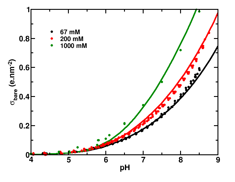
Figure 1: Comparison of experimental and simulated bare surface charge density versus pH for silica in aqueous solution at different NaCl concentrations. The simulations are represented by solid lines, the experimental data by points. The salt concentrations are 67 mM (black), 200 mM (red), 1000 mM (green). The experimental data are from Dove et al.Dove and Craven (2005).

Figure 1 presents the titration curve of silica in NaCl salt solution at three different concentrations, these data were obtained by Dove et al. Dove and Craven (2005). The charge density (in absolute values) increases with increasing pH due to the progressive dissociation of the silanol groups. $\sigma$ is also seen to increase with the salt concentration as a result of a greater screening of the electrostatic repulsion between charged sites. The following set of parameters, p$K_{a}$ = 7.7, $d_{site}$ = 5.55 nm^-2 and $\lambda_{Stern}$ = 0.107 nm, is found to provide a good description of the charging process of silica. Note that these parameters were obtained with Eq. 32 assuming a planar surface in the limit of infinite dilution. They are kept constant in the rest of the manuscript. The surface charge densities of a planar silica surface for several pH values and conditions used throughout this study are given in Table 1.

pH	Surface charge ($\text{e.nm}^{-2}$)
7	0.0816
8	0.18
9	0.365
9.5	0.508
10	0.695
10.5	0.932

Table 1: pH and bare surface charge density calculated for a planar silica surface in a monovalent salt solution with $c_{s}=5\text{ mM}$, $\lambda_{B}=0.7105\text{ nm}$, $pKa=7.7$, $d_{site}=5.55\text{ nm}^{-2}$, $\lambda_{Stern}=0.107\text{ nm}$.

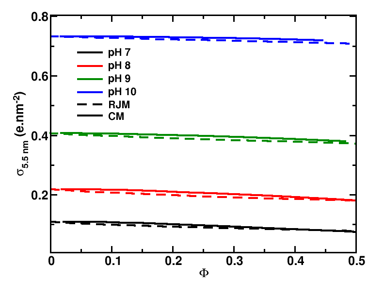
Figure 2: Calculated bare surface charge density for silica particles with $R_{p}$ = 5.5 nm when varying the particle volume fraction of a polydisperse HS40 suspension in monovalent salt solution at different pHs: 7 (black), 8 (red), 9 (green), and 10 (blue). The results are presented both with the polydisperse CM (solid lines) and RJM (dashed lines) approximations. The salt concentration is set to 5 mM.

$\sigma$ titrates with pH but also regulates as the particle volume fraction increases. The drop of $\sigma$ with $\psi$ is illustrated in Fig. 2 for the particle family of radius 5.5 nm in an HS40 suspension (polydispersity 14%) dispersed in a monovalent salt solution. This trend is similar in the PCM and PRJM and is explained by the co-ion exclusion which effectively mimics the strong interactions of the colloidal particles with their neighbors. The calculated $\sigma$, although close, tends to be larger within the PCM than the PRJM. This discrepancy increases as the pH is depressed ($<$10% at pH 7, and $<$1% at pH 10).

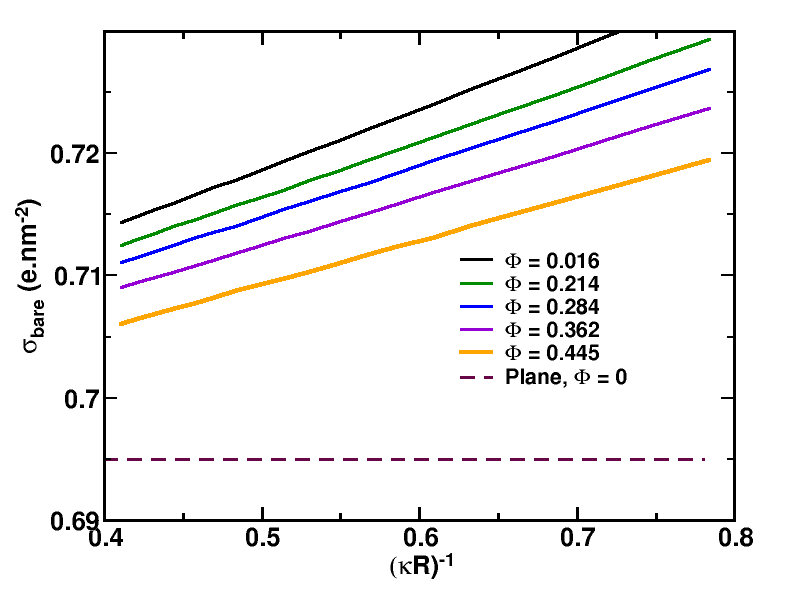
(a)  CM

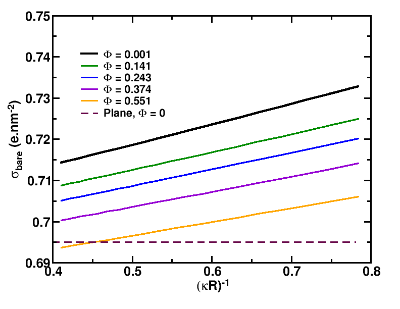
(b)  RJM

Figure 3: Bare surface charge $\sigma$ versus dimensionless curvature $(\kappa R)^{-1}$ at pH 10 and several volume fractions (see legend), for the PCM (a) and the PRJM (b). The surface charge for a planar surface at infinite dilution ($\Phi=0$) are displayed in both cases with a purple dashed line.

A result of the charge titration is also the curvature dependence of the particle charging. In particular, Abbas and coworkersAbbas et al. (2008) showed that there is a considerable increase in the surface charge density for particles smaller than 10 nm in diameter. The rise in charge up with particle curvature can be understood as an enhanced screening of small sized particles by counter-ions as compared to that of large particles. This is illustrated in Fig. 3 as a function of the dimensionless curvature $(\kappa R_{p})^{-1}$ at pH=10 for various $\Phi$ of the HS40 silica particle dispersion. The calculations are performed both in the PCM and PRJM approximations and are compared to the planar case at infinite dilution. Interestingly, the curvature dependence of $\sigma$ is found to vary linearly with $(\kappa R_{p})^{-1}$. This can be explained by the Taylor development of $\sigma$ with respect to $(\kappa R_{p})^{-1}$ which in the limit of $\kappa R_{p}\gg 1$ takes the form

$$\sigma(R_{p})=\sigma_{plane}(1+A_{0}(\kappa R_{p})^{-1}),$$ (35)

where $\sigma_{plane}$ is the charge density of a planar surface and $A_{0}$ gives the slope. Note that here it also applies to relatively small $(\kappa R_{p})^{-1}$. It should be mentioned, however, that in the pH region of large charge regulation, typically for pH values close to p$K_{a}$ Lund and Jönsson (2005), the linear relationship only holds for $\kappa R_{p}>2$, not shown. The slope of $\sigma(1/\kappa R_{p})$ is seen to decrease slightly with the particle volume fraction as a result of increasing counter-ion screening which tends to moderate, in relative terms, that due to curvature. Also, in the large $\Psi$ domain, the $\sigma$ of the small particles becomes lower than $\sigma_{plane}$ in the reference state (i.e. $\Psi=0$), see e.g. Fig. 3-b. In the infinite dilution limit where a Grahame relation for the nonlinear PBE in the spherical geometry has been recently obtained de Carvalho, Metzler, and Cherstvy (2016), an analytical expression for $A_{0}$ can be found. It reads

$$A_{0}=\frac{\frac{1}{\cosh^{2}(\psi_{0,plane}/4)}+\frac{C\sigma_{plane}\kappa\lambda_{Stern}}{2q_{s}\tanh(\psi_{0,plane}/2)}}{1+\frac{1/(1-\alpha_{plane})+C\sigma_{plane}}{2q_{s}\tanh(\psi_{0,plane}/2)}}.$$ (36)

A detailed development is given in the SI.

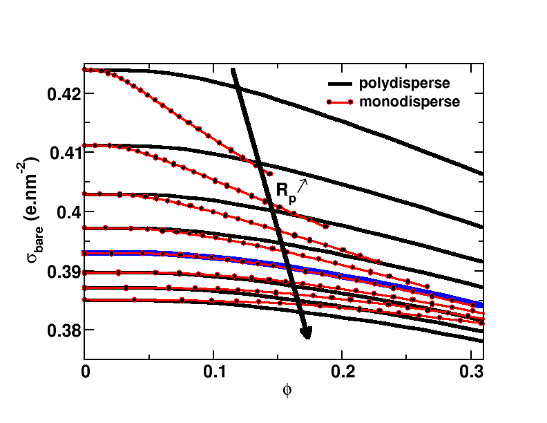
(a)  

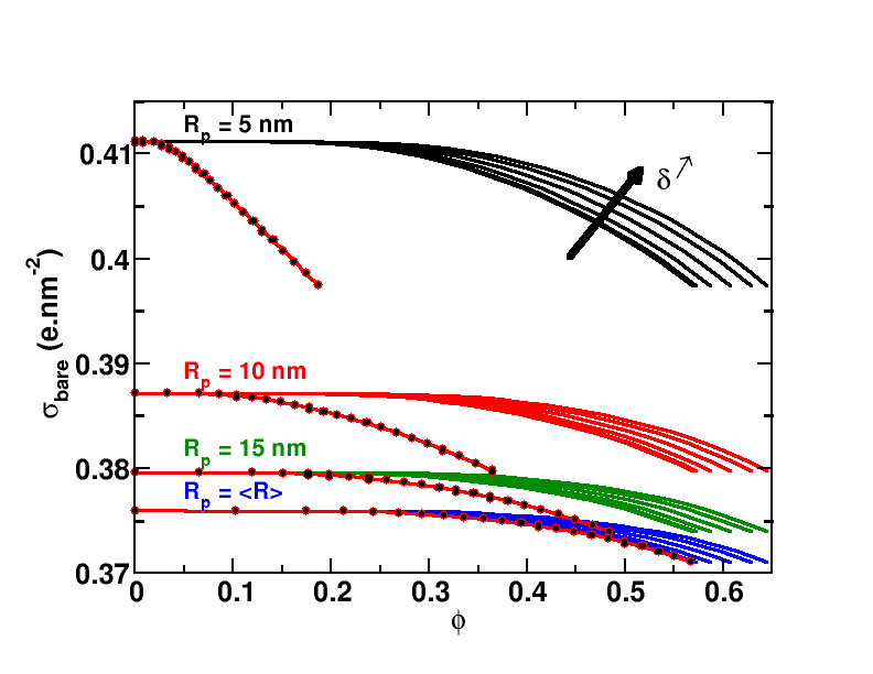
(b)  

Figure 4: Bare surface charge density, $\sigma$, for particle suspensions immersed in a 5 mM 1-1 salt solution at pH 9 for various particle sizes, size distributions and particle volume fractions a) $\sigma$ for particles of various $R_{p}$ (4, 5, 6, 7, 8, 9, 10 and 11 nm) within HS40 suspensions in comparison with the corresponding monodisperse cases. The blue line gives that of particles with $R_{p}=\langle R_{p}\rangle$. b) The same as in (a) but for particle suspensions having a normal radii distribution with $\langle R_{p}\rangle$ = 20 nm at different polydispersities $\delta$ (5, 10, 20, 30, 40 and 50 %). $\sigma$ of monodisperse particle suspensions (red lines with symbols) are also given for comparison.

The influence of polydispersity on the bare surface charge density of different particle families, i.e. with different $R_{p}$, is illustrated in Fig. 4 which compares the case of polydisperse and monodisperse suspensions for various particle size distributions. Interestingly, for particles with $R_{p}$ equal to the mean value of the distribution, $R_{p}=\langle R_{p}\rangle$, the polydispersity, when it is relatively small ($<$15%), has virtually no impact on $\sigma$. As could be expected, this is the same for infinitely diluted suspensions whatever the particle family or polydispersity, see Fig. 4-b. On the contrary, as $R_{p}$ departs from $\langle R_{p}\rangle$, the $\sigma$ of mono- and poly-disperse suspensions can clearly be seen to differentiate and this differentiation steps up with $\Phi$ and the departure from $\langle R_{p}\rangle$. The polydispersity effect is more pronounced for the small particles of the size distribution. In addition, polydispersity yields them higher charges (compared to monodispersity) which monotonically increase with it. The opposite is found for the large particles.

III.2 Renormalized parameters

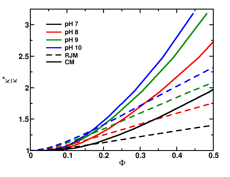
(a)  

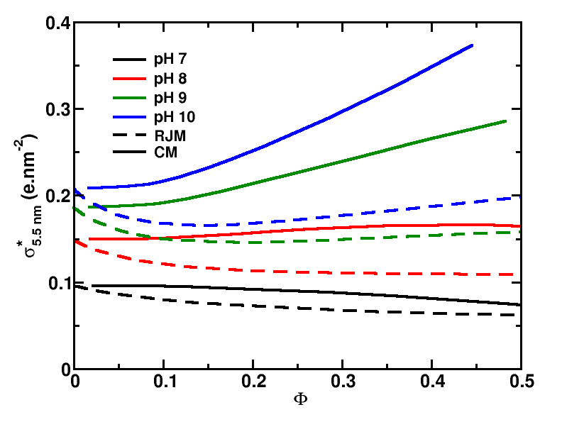
(b)  

Figure 5: a) Relative effective inverse screening length $\kappa^{\ast}/\kappa$, and b) effective surface charge density $\sigma^{\ast}$ versus volume fraction $\Phi$, for particles with $R_{p}=$5.5 nm of the HS40 dispersion, at the following pHs: 7 (black), 8 (red), 9 (green) and 10 (blue). The ionic strength is set to 5 mM. The full lines give the results of the PCM while the dashed lines those of the PRJM.

So far we have seen that the bare surface charge densities as obtained from the PCM and PRJM approximations are very similar whatever the particle size distribution or particle volume fraction. This is no longer true for the renormalized charge and screening length as shown in Fig.5. These parameters are calculated for HS40 suspensions at various $\Phi$.

$\sigma^{\ast}$ obtained within the PRJM is found to be lower than that within the PCM, whatever the $\Phi$ and all the more so as pH increases, that is as the effective charge approaches saturation. The same is observed for $\kappa^{\ast}$ but in the domain of large $\Phi$ ($\Phi\gtrsim 0.15$) while the opposite is found, that is $\kappa^{\ast}_{RJM}>\kappa^{\ast}_{CM}$, in the dilute and semi-dilute regimes ($\Phi\lesssim 0.15$). These results are consistent with those obtained by Trizac et al. with monodisperse suspensions, see Refs Trizac and Levin, 2004; Dobnikar et al., 2006, but are here exacerbated by the polydispersity. In particular, $\kappa^{\ast}$ values of both models are found not to converge in the limit of large $\Phi$, the domain of counter-ion dominated systems (supposedly equivalent to the salt free case), but, instead, to become increasingly divergent even at low pH values. Note that in the salt free case (not shown), $\sigma^{\ast}$ is still distinctly lower in the RJM, but the $\kappa^{\ast}$ of both models are found to be similar in the domain of low $\Phi$ ($<0.2$).

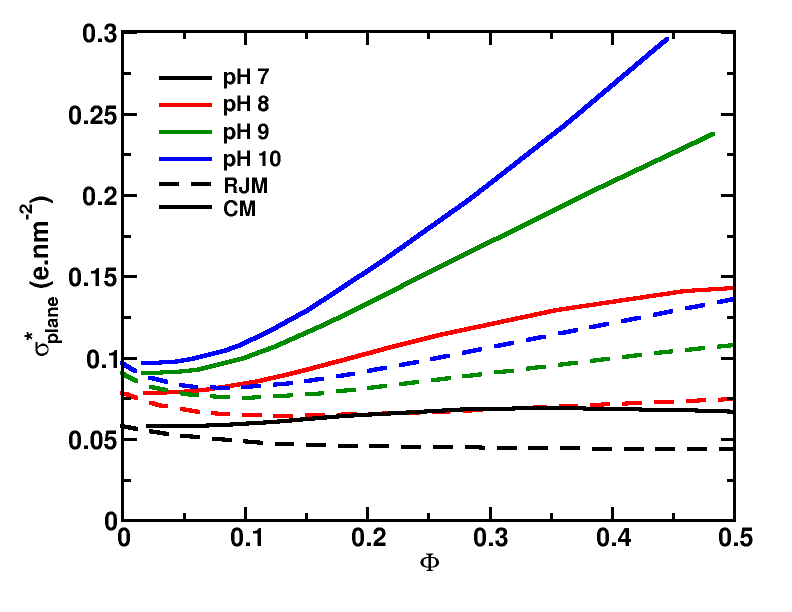
(a)  

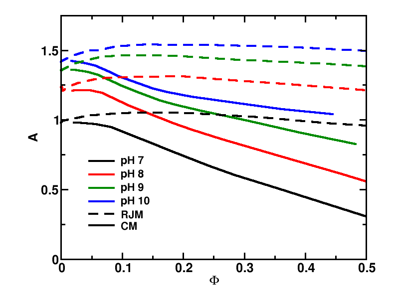
(b)  

Figure 6: Effective charge density of the planar surface $\sigma^{\ast}_{plane}$ and factor $A$ versus volume fraction $\Phi$. Those were worked out for the HS40 distribution, and for the following pHs: 7 (black), 8 (red), 9 (green), and 10 (blue), using the PCM (full lines), and the PRJM (dashed lines) .

In the same way as for the bare charge density, the effective surface charge density can be accurately approximated by means of an affine function of $(\kappa^{\ast}R_{p})^{-1}$, that is,

$$\sigma^{\ast}=\sigma^{\ast}_{plane}\left(1+A(\kappa^{\ast}R_{p})^{-1}\right),$$ (37)

where $\sigma^{\ast}_{plane}$ is the effective surface charge density of the confined planar surface in the same conditions (pH and $\Phi$, i.e. same edge potential for the PCM and same background charge for the PRJM) and $A$ is a dimensionless coefficient which measures the impact of the size of the particle. $\sigma^{\ast}_{plane}$ and $A$ depend on the model, pH, particle size distribution and volume fraction. Equivalently, Eq. 37 can be written in terms of effective charge, that is $Z^{\ast}/R_{p}=4\pi\sigma^{\ast}_{plane}/\kappa^{\ast}(\kappa^{\ast}R_{p}+A)$. In the case of no added salt, after noting that $\sigma^{\ast}=\frac{\gamma\kappa^{\ast}}{\pi\lambda_{B}}$, where $\gamma$ is a coefficient which varies with $\sigma$ and $\Phi$ Bocquet, Trizac, and Aubouy (2002), it was found that $Z^{\ast}$ scales linearly with the ratio $R_{p}/\lambda_{B}$. Such linear scaling was verified experimentally for deionized colloidal suspensions in the infinite dilution limit, in the semi-dilute regime and in the concentrated regime by measurements of electrophoretic mobility of isolated colloidsGarbow et al. (2004); Strubbe, Beunis, and Neyts (2006), conductivity of colloidal liquids and elasticity of colloidal crystalsWette, Schöpe, and Palberg (2002), respectively.

In the case of added salt ($\kappa R_{p}\gg 1$) and infinite dilution limit, where an analytical expression of the electrostatic potential solution of the non linear Poisson Boltzmann theory has been obtained Shkel, Tsodikov, and Record (2000); Aubouy, Trizac, and Bocquet (2003), an analytical approximation of the coefficient A for non titrating colloids can be obtained and reads,

$$A=\frac{1}{2}\left(5-\frac{\gamma^{4}+3}{\gamma^{2}+1}\right),$$ (38)

where $\gamma=\sqrt{1+x^{2}}-x$ and $x=\frac{\kappa}{2\pi\lambda_{B}\sigma}$. The approximation is asymptotically exact in the limit of large R, see the SI for a detailed development. Finally, since $\gamma$ goes to 1 when $\sigma\rightarrow\infty$ one finds $A_{sat}=3/2$ at the saturation of the colloidal charge.

Fig. 6 shows the PCM and PRJM results of the coefficient A and the effective charge density of the plane, $\sigma^{\ast}_{plane}$, versus $\Phi$ on HS40 at different pH and a set ionic strength of 5 mM. Not surprisingly, $\sigma^{\ast}_{plane}$ follows the same trend as for $\sigma^{\ast}_{5.5\text{ nm}}$, c.f. Fig. 5(b). In particular, for pH values greater than the p$K_{a}$ (pH $>7.7$) PRJM’s $\sigma^{\ast}_{plane}$ systematically shows a non monotonous behavior with respect to $\Phi$ with a minimum around $\Phi\approx 0.1$. Within the PCM, on the other hand, $\sigma^{\ast}_{plane}$ continuously rises with $\Phi$. The difference in behavior in $\sigma^{\ast}_{plane}$ between the two models is reminiscent of that of $\sigma^{\ast}_{plane}$ at saturation which follows the same qualitative trend, see e.g. Ref. Pianegonda, Trizac, and Levin, 2007. Indeed, in these conditions of pH, $\sigma_{plane}$ is generally larger than $\sigma^{\ast}_{plane,sat}$. For pH values lower than the p$K_{a}$ and at relatively high $\Phi$ the PCM’s $\sigma^{\ast}_{plane}$ also shows a drop due to the regulation of the bare charge density which becomes much smaller than $\sigma^{\ast}_{plane}$ at saturation.

This qualitative difference is echoed in the coefficient $A$ which shows a maximum value in the PRJM and not in the PCM, see Fig. 6-b. Indeed, $A$ varies between a maximum value $A_{sat}$, at the saturation of the charge and a minimum value $A_{0}$ when $\sigma^{\ast}=\sigma$, c.f. Eq. 35. It naturally follows that $\sigma^{\ast}(R_{p})$ desaturates as $\Phi$ further increases and approaches the ideal planar limit where the effective charge is proportional to $R_{p}^{2}$. In this respect, the PCM’s $A$ values decrease faster with $\Phi$ than is the case in the PRJM. In addition, for non titrating surfaces $A_{0}=0$ ($\sigma(R_{p})=\sigma_{plane}$) and, as we have seen above, $A_{sat}\leavevmode\nobreak\ 1.5$ at $\Phi=0$ both for titrating and non titrating surfaces.

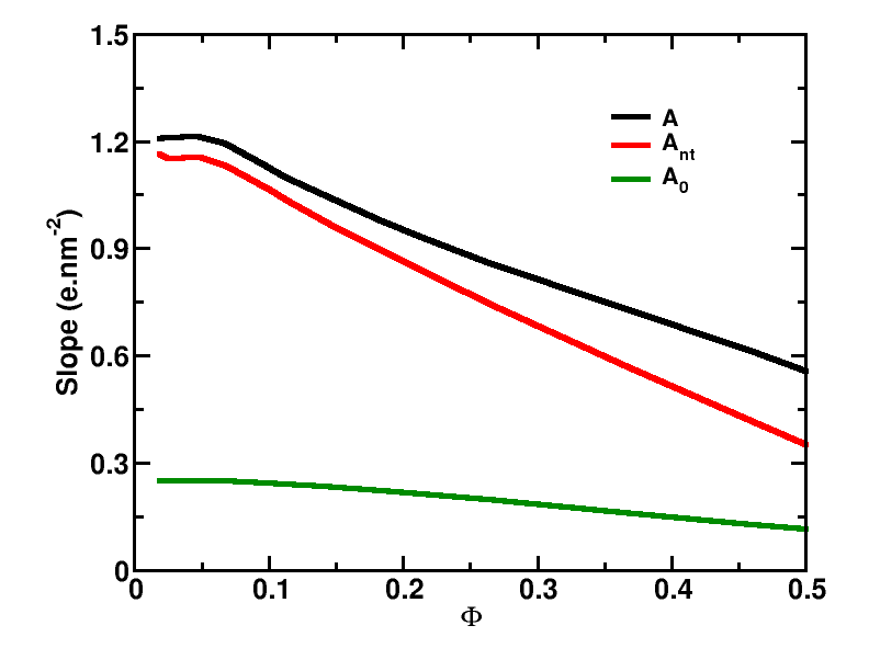
(a)  CM

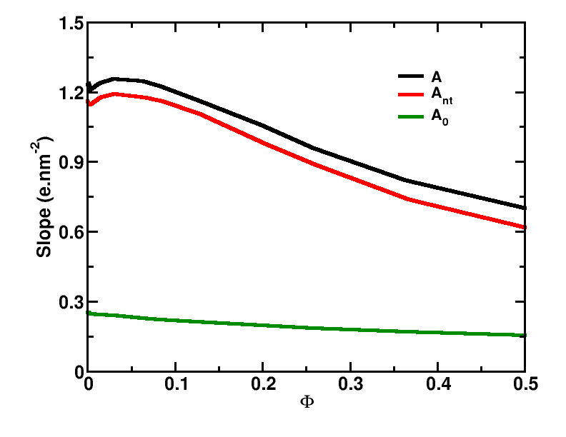
(b)  RJM

Figure 7: Slopes of the linear variation of $\sigma^{\ast}$ with $(\kappa R_{p})^{-1}$ of a titrating, $A$, and a non-titrating colloidal particle, $A_{nt}$. That of the bare surface charge density, $A_{0}$, is also given as a reference. The slopes are given for both the PCM (a) and PRJM (b). Calculations are performed for silica HS40 dispersions in equilibrium with a bulk solution containing 5mM of 1-1 salt and at pH 8. In the non titrating case, the particles are given a surface charge density equal to that of the planar silica surface in the same conditions.

This points to the fact that for non titrating colloids, with a $\sigma(R_{p},\Phi)$ equal to that of a titrating planar surface in the same conditions ($\sigma_{plane}(\Phi,\mathrm{pH})$), the corresponding coefficient, $A_{nt}$, is lower than $A$ for charge regulating particles. In other words, $A$ is a function of $A_{0}$ and $A_{nt}$, see Figure 7. In the limit of small variations of $\sigma$, one can further give an analytic approximation for the dependence of $A$ on $A_{0}$ and $A_{nt}$ which reads,

$$A\approx A_{nt}+\frac{\kappa^{\ast}}{\kappa}A_{0}\frac{\sigma_{b}}{\sigma^{\ast}}\frac{\mathrm{d}\sigma^{\ast}}{\mathrm{d}\sigma_{b}}.$$ (39)

Close to the saturation of the effective charge as well as in the limit of small $\sigma_{p}$ the last expression reduces to $A\approx A_{nt}+\kappa^{\ast}/\kappa A_{0}$.

Not shown here is how the ionic strength affects both $\sigma^{\ast}_{plane}$ and $A$. This is already well documented in the literature in the case of monodisperse suspensions, see e.g. Refs. Belloni, 1998; Groot, 1991; Stevens, Falk, and Robbins, 1996. Not surprisingly, the same qualitative behavior is found in polydisperse suspensions. That is, $A$ drops and $\sigma^{\ast}$ rises when ionic strength increases. It is also is easy to infer from Eqs. 8-22 and Fig. 4 that an increase in the polydispersity gives rise to a shift in $\sigma^{\ast}_{plane}$ and $A$ values to larger $\Phi$ values.

In conclusion of this section, we have seen that the well-known linear scaling of the effective charge with $(\kappa R_{p})^{-1}$ is also verified in the case of polydisperse and charge regulating colloids for all $\Phi$. In practice, this means that a complete force field for these suspensions can be obtained at relatively low computational cost. Indeed, this amounts to calculating $A$, $\sigma^{\ast}_{plane}$ and $\kappa^{\ast}$ with a few $R_{p}$ values (in principle two are enough) at set values of $\psi_{c}$ (in the PCM) or $Z_{back}$ (in the PRJM), and post-calculating $\Phi$ given the particle size distribution (continuous or not).

III.3 Osmotic pressure

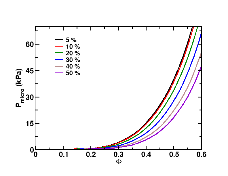
Figure 8: Simulated microion contribution to the osmotic pressure of titratating silica particle dispersions as a function of the particle volume fraction for varying polydispersities. The calculations are performed within the PCM approximation. The silica particles are suspended in a 5 mM 1-1 salt solution at pH 9. The particles present a normal size distribution with $\langle R_{p}\rangle=$ 20 nm. The polydispersity is changed as indicated in the legend.

In this section the effect of the polydispersity on osmotic pressure is discussed. Finally, the validity of the PRJM and PCM will be discussed in light of experimental equation of states for various commercial silica dispersions.

Figure 8 gives the microion contribution to the total osmotic pressure, $P_{micro}$ as obtained from the PCM with different polydisperse suspensions having a normal size distribution of the same mean particle size $\langle R_{p}\rangle=$ 20 nm but of varying polydispersities. $P_{micro}$ is found to decrease as $\delta$ increases. The drop in $P_{micro}$ is significant above 10% of polydispersity. The PRJM exhibits the same qualitative behavior (not shown).

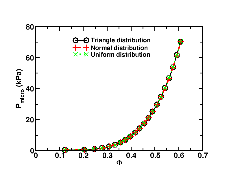
(a)  

(b)  

Figure 9: (a) CM calculations of the micro-ions osmotic pressure, $P_{micro}$, for silica dispersions with varying shapes of particle size distribution but with identical $\langle R_{p}\rangle$ (20 nm) and $\langle R_{p}^{3}\rangle$ (21.77³ nm³). The silica particles are suspended in a 5 mM 1-1 salt solution at pH 9. Note that for the normal distribution $\delta=31\%$. The distribution is changed as indicated in the legend. (b) The triangular, normal and uniform size distributions used.

The shape of the particle radius distribution is further found to have only a minor effect on $P_{micro}$. This is all the more true as the particle size distributions are chosen so as to have identical $\langle R_{p}^{3}\rangle$ and $\langle R_{p}\rangle$. As shown in Figure 9-a for three different distribution shapes, when these conditions are met the $P_{micro}$ thus obtained can hardly be distinguished. This behavior is a direct consequence of the geometrical definition of the particle volume fraction, see Eq. 6 combined with the very slow variation in the water layer thickness, $R_{cell}-R_{p}$, with the particle radius. In the limit of large $\kappa R_{p}$, $R_{cell}-R_{p}$ becomes constant.

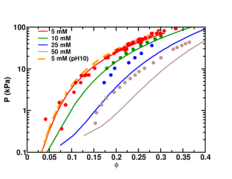
(a)  

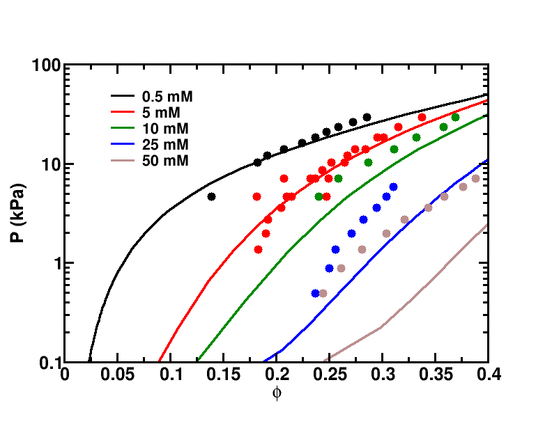
(b)  

Figure 10: Experimental equation of state for the (a) HS40 and (b) TM50 silica dispersions in comparison with the micro-ion pressure calculated by the polydisperse cell model at various bulk concentrations of monovalent salt and pH 9. The results for the polydisperse RJM are given in the SI.

Fig. 10 compares the experimental equations of state of the HS40 and TM50 silica dispersionsGoehring, Li, and Kiatkirakajorn (2017) with the micro-ion pressure calculated with the polydisperse cell model at various bulk concentrations of monovalent salt and pH 9. The osmotic pressure is seen to increase when the ionic strength of the bulk and the mean particle radius ($\langle R_{p}(\text{HS40})\rangle<\langle R_{p}(\text{TM50})\rangle$) decreases, in good agreement with the polydisperse cell model. What is more, the PCM is found to give a good description of the osmotic pressure of the silica dispersions only for the lowest bulk salt concentrations studied, up to 10 mM for the HS40 and to 5 mM for the TM50. This should not come as a surprise since the PCM is known to neglect the entropic and contact contributions to the osmotic pressureHallez, Diatta, and Meireles (2014); Dobnikar et al. (2006). As discussed by Hallez et al.Hallez, Diatta, and Meireles (2014) , it is found that the lower the mean particle size, the larger the validity range of the PCM. The PRJM, on the other hand, is found to give a poor description of the experimental osmotic pressure, see SI. Generally, it overestimates the osmotic pressure at low volume fractions and underestimates them in the concentrated regime.

IV Conclusion

In this paper, we proposed a cell and a renormalized jellium model to study the thermodynamic properties and estimate the renormalized parameters to be used in a one-component model, i.e. $Z^{\ast}$ and $\kappa^{\ast}$, for polydisperse suspensions of titratable spherical colloids with a continuous size distribution. We further proposed a simple algorithm and a Nim implementation to solve them. The models are largely inspired by the work of TorresTorres, Téllez, and van Roij (2008) on binary mixtures of colloids with constant charge. PCM and PRJM include a charge regulation, instead of a constant charge boundary condition, modeled as a simple 1-p$K$-Stern model. The application of the models to continuous size distributions was made simple and easy by the linear scaling of both the bare and effective charges with the adimensional curvature of the particles, $(\kappa R_{p})^{-1}$. For very small $(\kappa R_{p})^{-1}$, $\sigma$ and $\sigma^{\ast}$ scale quadratically. We presented a detailed example of such an analysis in the case of aqueous suspensions of silica nanoparticles of various size distributions. Besides being simple, the 1-p$K$ model was found to give a very good description of the charging behavior for bare silica surfaces experimentally observed in diluted conditions, in accordance with previous studies, see e.g. Ref. Kobayashi et al., 2005. This allowed us to constrain the surface chemistry parameters of the PCM, leaving us with two commonly characterized parameters, that is the pH and the particle size distribution. Both models give the same qualitative results. Yet, the cell model thus generalized is found to predict much more accurately the equations of state of aqueous silica dispersions at finite salt concentrations. In general, the bare surface density is found to drop as the density and the radius of the silica particles increases, due to the charge regulation. In a polydisperse suspension, the particles of radius $R_{p}<\langle R_{p}\rangle$ are further found to bear a surface charge density significantly greater than that of the same particles at the same density but in a monodisperse suspension (the opposite occurs when $R_{p}>\langle R_{p}\rangle$). This is all the more true as polydispersity rises and $R_{p}$ is small compared to $\langle R_{p}\rangle$ ($R_{p}>>\langle R_{p}\rangle$). In other words, the bare charge polydispersity is found to increase with the size polydispersity. Not surprisingly, the same trend is found for the effective charge polydispersity. It should be stressed, however, that a polydispersity of effective charges is also present in the case of polydisperse particles having the same bare surface charge density, although less pronounced. Despite these differences a significant impact on the microion osmotic pressure is only seen in suspensions of silica particles with very large polydispersities ($>15\%$). One may expect, however, to observe more clear effects in the micro-structure of these suspensions, even for relatively small polydispersities.