Massive quark form factors

Abstract:

In this contribution we provide further details to the recent calculation of QCD corrections to massive three-loop form factors presented in Ref. [1].

1 Introduction

Form factors play an important role in any quantum field theory. They are building blocks for various physical quatities and furthermore provide a playground for studying infrared properties. In this contribution form factors involving massive quark are discussed. The most advanced results have been obtained in Refs. [1] and [2], where three-loop corrections have been considered. More precisely, all light-fermion contributions have been computed and the non-fermionic part has been considered in the large-$N_{c}$ limit. In the latter case only planar Feynman diagrams contribute whereas in the former case also non-planar integral families have to be taken into account. For references to previous work, in particular to two-loop calculations, we refer to [1].

In this contribution we provide more details to the calculation performed in Ref. [1]. Furthermore, numerical results are presented for the imaginary part of the form factors.

2 Quark form factors

We consider QCD correction to the interaction of massive quarks with a vector, axial-vector, scalar or pseudo-scalar current defined as

$$j_{\mu}^{v} = \bar{\psi}\gamma_{\mu}\psi\,,$$

$$j_{\mu}^{a} = \bar{\psi}\gamma_{\mu}\gamma_{5}\psi\,,$$

$$j^{s} = m\,\bar{\psi}\psi\,,$$

$$j^{p} = im\,\bar{\psi}\gamma_{5}\psi\,.$$ (1)

The tensor decomposition of the corresponding vertex functions leads to six scalar functions which we define as

$$\Gamma_{\mu}^{v}(q_{1},q_{2}) = F_{1}^{v}(q^{2})\gamma_{\mu}-\frac{i}{2m}F_{2}^{v}(q^{2})\sigma_{\mu\nu}q^{\nu}\,,$$

$$\Gamma_{\mu}^{a}(q_{1},q_{2}) = F_{1}^{a}(q^{2})\gamma_{\mu}\gamma_{5}{-\frac{1}{2m}F_{2}^{a}(q^{2})q_{\mu}}\gamma_{5}\,,$$

$$\Gamma^{s}(q_{1},q_{2}) = {m}F^{s}(q^{2})\,,$$

$$\Gamma^{p}(q_{1},q_{2}) = {im}F^{p}(q^{2}){\gamma_{5}}\,.$$ (2)

$F_{1}^{v},\ldots,F^{p}$ depend on the ratio of the virtuality $q^{2}$, where $q$ is the outgoing momentum of the external current, and the square of the heavy quark mass $m$. For the practical calculation it is convenient to introduce the variable $x$ defined through

$$\frac{q^{2}}{m^{2}} = -\frac{(1-x)^{2}}{x}\,,$$ (3)

which maps the complex $q^{2}/m^{2}$ plane into the unit circle. In particular, we have that the special points $q^{2}=0$, $q^{2}=4m^{2}$ and $q^{2}\to\-\infty$ are mapped to $x=1,-1$ and $0$, respectively.

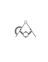
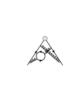
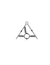
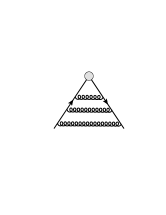
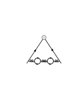
Figure 1: Sample diagrams contributing to the form factors. Solid and curly lines represent quarks and gluons, respectively. The grey blob refers to one of the external currents given in Eq. (1).

The workflow of our calculation is as follows: We generate the amplitudes using qgraf [3]. Althogether 337 diagrams are generated, which, however, also includes non-planar integrals. We use color to compute the colour factors which allows us to select the fermionic and large-$N_{c}$ contributions. Representative three-loop diagrams can be found in Fig. 1. We use q2e [4, 5] to transform the qgraf output to FORM [6] notation and exp [4, 5] together with the underlying symmetries of the vertex diagrams to map all contributing integrals to eight planar and three non-planar integral families (see Fig. 1 of Ref. [7] and Fig. 5 of Ref [1] for graphical representations).

In a next step we compute the amplitudes of each Feynman diagram using FORM [6]. We apply projectors to obtain the scalar function $F_{1}^{v},\ldots,F^{p}$, take traces and map each integral to a scalar function as defined by the corresponding integral family. For most diagrams this step takes only a few minutes for a general QCD gauge parameter. Afterwards we extract the integral list which serves as input for FIRE [8]. FIRE is used in combination with LiteRed [9, 10] for the reduction to master integrals. For the large-$N_{c}$ contribution we have ${\cal O}(10^{5})$ and for the $n_{l}$ term about $30\,000$ integrals. For the most complicated integral family the reduction to master integrals takes of the order of a week on a 12-core node with main memory of order 100 gigabyte.

Analytic results for the master integrals are available from Refs. [7] (89 planar integrals) and [11] (additional 15 integrals, two of them are non-planar), respectively. They are used to express each of the six form factors $F_{1}^{v},\ldots,F^{p}$ in terms of Goncharov polylogarithms (GPLs) [12]. Computer-readable expressions can be found in the ancillary file to Ref. [1]. They are quite lengthy, however, a numerical evaluation is possible with the help of ginac [13, 14].

There are several checks on the correctness of our result: First of all, we have verified that in the renormalized form factors the QCD gauge parameter drops out. We also obtain the expected limiting behaviours for $x\to 0,1,-1$ (see Ref. [1] for an extensive discussion). Furthermore, we can check the pole part against a dedicated calulation of the cusp anomalous dimension $\Gamma_{\rm cusp}$ which has been performed in Ref. [15]. Note that we obtain the same result for $\Gamma_{\rm cusp}$ for all four currents of Eq. (1) which is expected due to the universality of the infra-red behaviour. Finally, we obtain complete agreement for the renormalized three-loop form factors $F_{1}^{v},\ldots,F^{p}$ with an independent calculation performed in Ref. [2]. Let us stress that in [2] different software has been used to perform the reduction to master integrals, the integral families are defined differently and a different method has been used to compute the master integrals.

3 Numerical results

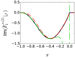
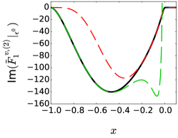
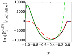
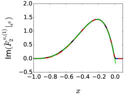
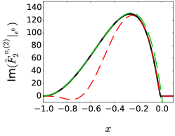
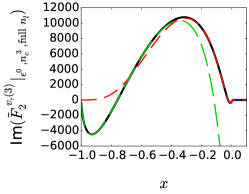
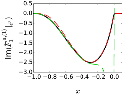
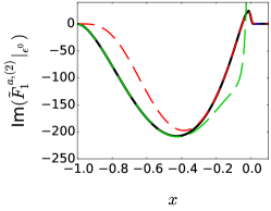
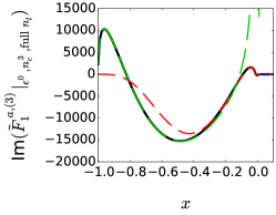
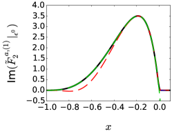
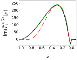
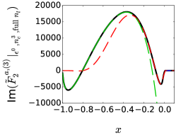
Figure 2: Imaginary part of the $\epsilon^{0}$ term of the vector and axial-vector form factors as a function of $x$. Exact results and approximations are shown as solid and dashed lines, respectively. At three-loop order we add the complete light-fermion part for $n_{l}=5$ and the $N_{c}^{3}$ contribution. Medium- (red) and long- (green) dashed lines correspond to the high-energy and threshold approximation, respectively. Note that the imaginary part is zero for $x\in[0,1]$.

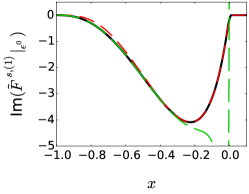
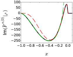
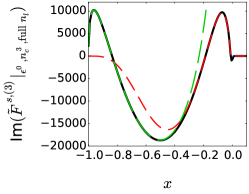
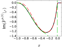
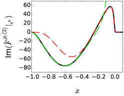
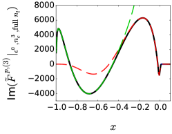
Figure 3: Same as Fig. 2 but for the the scalar and pseudo-scalar currents.

We refrain to show analytic expressions but refer to [7, 1, 1] for analytic results in the kinematic limits $x\to 0,1$ and $-1$. In the following we complement the numerical results shown in [1] by discussing the imaginary parts of $F_{1}^{v},\ldots,F^{p}$.

In [1] plots for the real part of the $\epsilon^{0}$ term of

$$\tilde{F}(q^{2})=(1+x)^{4}\left[F(q^{2})-F(q^{2})\Big{|}_{q^{2}\to\infty}\right]\,.$$ (4)

are shown for $x\in[-1,1]$. The subtraction term and the factor $(1+x)^{4}$ guarantee that in all three limis ($x\to 0,1,-1$) finite results are obtained. Furthermore, the six scalar functions $F_{1}^{v},\ldots,F^{p}$ are multiplied by $(\pi-\phi)^{4}$ and plotted against $\phi\in[0,\pi]$, where $x=e^{i\phi}$.

Note that for $x>0$ and for values of $x$ on the circumference of the unit circle the form factors are real-valued. Thus, in Figs. 2 and 3 we show the imaginary parts of $\tilde{F}_{1}^{v},\ldots,\tilde{F}^{p}$ for negative values of $x$. By construction (cf. Eq. (4)) the form factors are zero for $x=-1$ and $x=0$. The exact result is shown as solid black curve. Short- and long-dashed curves correspond to high-energy and threhold approximations where terms up to order $x^{6}$ and $\beta^{3}$ [with $x=2\beta/(1+\beta)-1$] are included. Note that in all cases (except for a small region around $x\approx-0.3$ for the two-loop result of $F_{1}^{v}$) the whole range $x\in[-1,1]$ can be covered by the approximations, i.e., for each $x$-value there is at least one of the dashed curves on top of the (black) solid line.

4 Outlook

There are several possible next steps towards the full massive three-loop form factors. A well-defined and gauge invariant subset is the singlet contributions where the coupling of the external current to the external fermions is mediated via gluons. Another subset is composed of all (non-singlet) contributions with a closed massive fermion loop. However, all these cases are significantly more involved which is mainly due to the occurrence of so-called elliptic sectors where differential equations cannot be transformed into a canonical form. This makes it probably necessary to resign on numerical methods, e.g., along the lines presented in Ref. [16].

References

- [1] R. N. Lee, A. V. Smirnov, V. A. Smirnov and M. Steinhauser, JHEP 1805 (2018) 187 doi:10.1007/JHEP05(2018)187 [arXiv:1804.07310 [hep-ph]].
- [2] J. Ablinger, J. Blümlein, P. Marquard, N. Rana and C. Schneider, Phys. Lett. B 782 (2018) 528 doi:10.1016/j.physletb.2018.05.077 [arXiv:1804.07313 [hep-ph]].
-
[3]
P. Nogueira,
J. Comput. Phys. 105 (1993) 279;
- [4] R. Harlander, T. Seidensticker and M. Steinhauser, Phys. Lett. B 426 (1998) 125 [hep-ph/9712228].
- [5] T. Seidensticker, hep-ph/9905298.
- [6] B. Ruijl, T. Ueda and J. Vermaseren, arXiv:1707.06453 [hep-ph].
- [7] J. M. Henn, A. V. Smirnov and V. A. Smirnov, JHEP 1612 (2016) 144 [arXiv:1611.06523 [hep-ph]].
- [8] A. V. Smirnov, Comput. Phys. Commun. 189 (2015) 182 [arXiv:1408.2372 [hep-ph]].
- [9] R. N. Lee, arXiv:1212.2685 [hep-ph].
- [10] R. N. Lee, J. Phys. Conf. Ser. 523 (2014) 012059 [arXiv:1310.1145 [hep-ph]].
- [11] R. N. Lee, A. V. Smirnov, V. A. Smirnov and M. Steinhauser, JHEP 1803 (2018) 136 doi:10.1007/JHEP03(2018)136 [arXiv:1801.08151 [hep-ph]].
- [12] A. B. Goncharov, Math. Res. Lett. 5 (1998) 497 [arXiv:1105.2076 [math.AG]].
- [13] C. W. Bauer, A. Frink and R. Kreckel, J. Symb. Comput. 33 (2000) 1 [cs/0004015 [cs-sc]].
- [14] J. Vollinga and S. Weinzierl, Comput. Phys. Commun. 167 (2005) 177 [hep-ph/0410259].
- [15] A. Grozin, J. M. Henn, G. P. Korchemsky and P. Marquard, JHEP 1601 (2016) 140 [arXiv:1510.07803 [hep-ph]].
- [16] R. N. Lee, A. V. Smirnov and V. A. Smirnov, arXiv:1709.07525 [hep-ph].
- [17] J. A. M. Vermaseren, Comput. Phys. Commun. 83 (1994) 45.
- [18] D. Binosi and L. Theussl, Comput. Phys. Commun. 161 (2004) 76 [arXiv:hep-ph/0309015].