Lattice QCD and the anomalous magnetic moment of the muon

Abstract

The anomalous magnetic moment of the muon, $a_{\mu}$, has been measured with an overall precision of 540 ppb by the E821 experiment at BNL. Since the publication of this result in 2004 there has been a persistent tension of $3.5$ standard deviations with the theoretical prediction of $a_{\mu}$ based on the Standard Model. The uncertainty of the latter is dominated by the effects of the strong interaction, notably the hadronic vacuum polarisation (HVP) and the hadronic light-by-light (HLbL) scattering contributions, which are commonly evaluated using a data-driven approach and hadronic models, respectively. Given that the discrepancy between theory and experiment is currently one of the most intriguing hints for a possible failure of the Standard Model, it is of paramount importance to determine both the HVP and HLbL contributions from first principles. In this review we present the status of lattice QCD calculations of the leading-order HVP and the HLbL scattering contributions, $a_{\mu}^{\rm hvp}$ and $a_{\mu}^{\rm hlbl}$. After describing the formalism to express $a_{\mu}^{\rm hvp}$ and $a_{\mu}^{\rm hlbl}$ in terms of Euclidean correlation functions that can be computed on the lattice, we focus on the systematic effects that must be controlled to achieve a first-principles determination of the dominant strong interaction contributions to $a_{\mu}$ with the desired level of precision. We also present an overview of current lattice QCD results for $a_{\mu}^{\rm hvp}$ and $a_{\mu}^{\rm hlbl}$, as well as related quantities such as the transition form factor for $\pi^{0}\to\gamma^{\ast}\gamma^{\ast}$. While the total error of current lattice QCD estimates of $a_{\mu}^{\rm hvp}$ has reached the few-percent level, it must be further reduced by a factor $\sim 5$ to be competitive with the data-driven dispersive approach. At the same time, there has been good progress towards the determination of $a_{\mu}^{\rm hlbl}$ with an uncertainty at the $10-15$%-level.

1 Introduction

The anomalous magnetic moment of the muon, $a_{\mu}$ is one of the most precisely measured quantities in particle physics. It is defined as the deviation of the $g$-factor, which determines the strength of the muon’s magnetic moment, from the value $g=2$ predicted by the Dirac equation, i.e.

$$g_{\mu}=2(1+a_{\mu}),\quad a_{\mu}=\frac{1}{2}(g-2)_{\mu}.$$ (1)

The deviation, caused by quantum loop corrections, is a characteristic property of the particle. Both $a_{\mu}$ and the corresponding anomalous magnetic moment of the electron, $a_{e}$, have been measured experimentally with very high precision [1, 2],

$$a_{\mu}^{\rm exp}=(116\,592\,089\pm 63)\cdot 10^{-11}\quad(540\,\rm ppb)$$ (2)

$$a_{e}^{\rm exp}=(115\,965\,218\,073\pm 28)\cdot 10^{-14}\quad(0.24\,\rm ppb)$$ (3)

The particular interest in $a_{\mu}$ comes from the high sensitivity to effects from physics beyond the Standard Model. The anomalous magnetic moment of a generic lepton, $a_{\ell}$, receives a contribution from quantum fluctuations induced by heavy particles proportional to

$$\delta a_{\ell}=m_{\ell}^{2}/M^{2},$$ (4)

where $m_{\ell}$ is the lepton mass, and $M$ denotes either the mass of a particle which is not part of the Standard Model (SM) or the energy scale beyond which the SM loses its validity. This implies that the sensitivity of $a_{\mu}$ to “new physics” is increased by a factor $(m_{\mu}/m_{e})^{2}\approx 4\cdot 10^{4}$ relative to $a_{e}$. Against this backdrop it is intriguing that there has been a persistent discrepancy between the measured value of $a_{\mu}$ and its prediction based on the SM, $a_{\mu}^{\rm exp}-a_{\mu}^{\rm SM}=(266\pm 76)\cdot 10^{-11}$, which amounts to $\sim 3.5$ standard deviations (see Table 1).

Within the SM, the anomalous magnetic moment of the muon receives contributions from QED, the electroweak sector, and the strong interaction:

$$a_{\mu}^{\rm SM}=a_{\mu}^{\rm QED}+a_{\mu}^{\rm EW}+a_{\mu}^{\rm had},$$ (5)

where the superscript “had” indicates that the effects of the strong interaction must be quantified at typical hadronic scales. An overview which specifies the contributions from electromagnetism, the weak and the strong interactions to $a_{\mu}$ is provided in Table 1. Extensive reviews of the subject, which detail the various contributions, can be found in Refs. [4, 5, 6].

	Value		Error		$a_{\mu}^{\rm exp}-a_{\mu}^{\rm SM}$
QED	11 658 471.	895	0.	008		10th order [7]
EW	15.	36	0.	11		Two loop [8, 9]
HVP, LO	693.	1	3.	4		DHMZ 17 [10]
HVP, NLO	$-9$.	84	0.	07		HMNT [11]
HLBL	10.	5	2.	6		PdeRV [12]
Total SM	11 659 182.	3	4.	3	$3.5\sigma$	DHMZ 17
Experiment	11 659 208.	9	6.	3		BNL E821 [1]

Table 1: Contributions to the SM prediction for $a_{\mu}$ from QED, the electroweak (EW) and hadronic sectors, in units of $10^{-10}$.

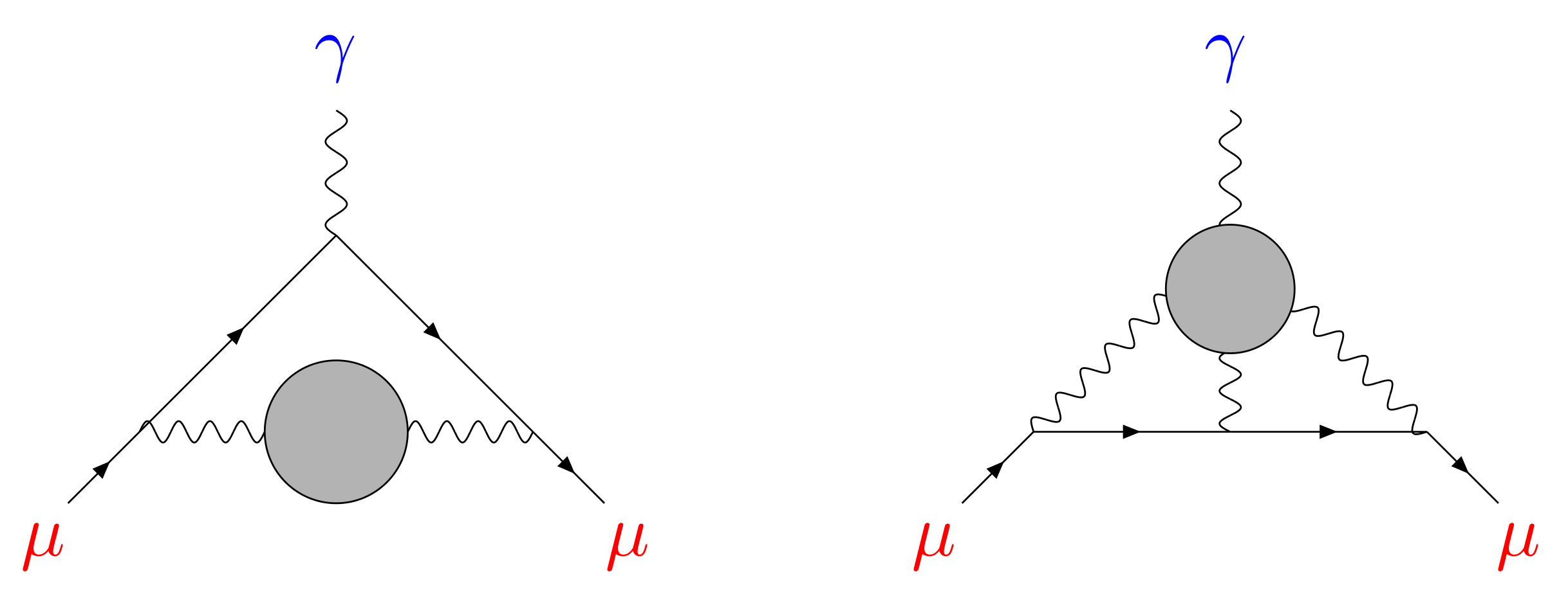
Figure 1: The diagrams representing the leading hadronic vacuum polarisation (left) and light-by-light scattering contributions. Grey circles denote the hadronic loops.

The overall precision of the SM prediction is limited by hadronic contributions, as is evidenced by Table 1. In particular, the uncertainties ascribed to the leading hadronic vacuum polarisation (HVP) and hadronic light-by-light (HLbL) scattering contributions (see Fig 1) dominate the total error of $a_{\mu}^{\rm SM}$. Efforts have therefore been concentrated on corroborating the actual estimates and reducing the associated uncertainties.

The leading (i.e. ${\rm{O}}(\alpha^{2})$) HVP contribution, $a_{\mu}^{\rm hvp}$, which enters the SM estimate has been determined via dispersion relations. In the conventions and notation of [4] the relevant expression reads

$$a_{\mu}^{\rm hvp}=\left(\frac{\alpha m_{\mu}}{3\pi}\right)^{2}\int_{m_{\pi^{0}}^{2}}^{\infty}ds\,\frac{\hat{K}(s)}{s^{2}}\,R(s),$$ (6)

where $\alpha$ is the fine-structure constant, $\hat{K}(s)$ is a known QED kernel function [13], and $R(s)$ denotes the cross section for $e^{+}e^{-}\to\hbox{hadrons}$ normalised by $\sigma(e^{+}e^{-}\to\mu^{+}\mu^{-})$ at tree level in the limit $s\gg m_{\mu}^{2}$:

$$R(s)=\frac{\sigma(e^{+}e^{-}\to\hbox{hadrons})}{4\pi\alpha^{2}/(3s)}$$ (7)

A high energies the ratio can be approximated with sufficient accuracy in perturbative QCD. However, at low energies, where the dispersion integral is dominated by the $\rho$-resonance, one has to resort to experimental data for $R(s)$. In practice one splits the integration into two intervals:

$$R(s)\longrightarrow\left\{\begin{array}[]{ll}R(s)^{\rm data},&m_{\pi^{0}}^{2}\leq s<E_{\rm cut}^{2}\\ R(s)^{\rm pQCD},&s>E_{\rm cut}^{2}\end{array}\right..$$ (8)

The resulting estimates for $a_{\mu}^{\rm hvp}$ from several independent analyses [14, 15, 16, 10, 17, 18] based on the combined data for $e^{+}e^{-}\to\hbox{hadrons}$ are listed in Table 2. Currently, several issues are still being debated: The first concerns the consistency of the experimental data in the $\pi^{+}\pi^{-}$ channel determined using the ISR (initial state radiation) method [19, 20, 21, 22, 23], as well as the treatment of this particular contribution in the evaluation of the dispersion integral. The second issue concerns the question whether a more precise result for $a_{\mu}^{\rm hvp}$ can be obtained by including data from hadronic $\tau$ decays in order to estimate the spectral function [24, 14, 15]. Progress has been achieved on both of these issues, and some of the most recent analyses of the SM contribution to $a_{\mu}$ report a slightly increased discrepancy of about $4\,\sigma$ with the direct measurement (see Table 2). While the dispersive approach produces estimates for $a_{\mu}^{\rm hvp}$ with a total error at the sub-percent level, it is clear that the resulting SM estimate is subject to experimental uncertainties. This is one of the main motivations for working towards a result based on a first-principles approach such as lattice QCD.

Author(s)	$a_{\mu}^{\rm hvp}\cdot 10^{-10}$		Error		$a_{\mu}^{\rm exp}-a_{\mu}^{\rm SM}$	Comment
DHMZ 11 [14]	692.	3	4.	2	$3.6\sigma$	$e^{+}e^{-}$ data
	701.	5	4.	7	$2.4\sigma$	$\tau$ data
FS 11 [15]	690.	75	4.	72		$e^{+}e^{-}$ data
	690.	96	4.	65	$3.3\sigma$	$e^{+}e^{-}$ and $\tau$ data
HLMNT 11 [16]	694.	9	4.	3	$3.2\sigma$	$e^{+}e^{-}$ data
DHMZ 17 [10]	693.	1	3.	4	$3.5\sigma$	$e^{+}e^{-}$ data
Jegerlehner 17 [17]	688.	07	4.	14	$4.0\sigma$	$e^{+}e^{-}$ data
	688.	77	3.	38	$4.1\sigma$	$e^{+}e^{-}$ and $\tau$ data
KNT 18 [18]	693.	27	2.	46	$3.7\sigma$	$e^{+}e^{-}$ data

Table 2: Compilation of results for the leading order (O($\alpha^{2}$)) hadronic vacuum polarisation contribution $a_{\mu}^{\rm hvp}$ from the data-driven dispersive approach.

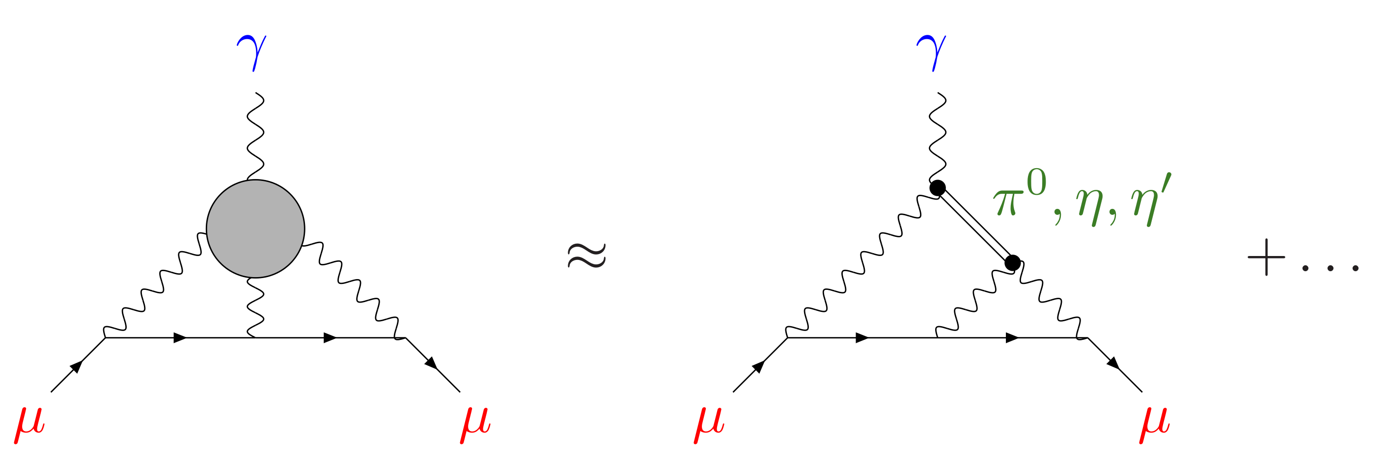
Figure 2: The expected dominant contributions to the HLbL scattering amplitude.

The hadronic light-by-light scattering contribution, $a_{\mu}^{\rm hlbl}$, has so far been determined via model estimates (see [25, 26, 27, 28, 29, 30, 31, 32, 4, 12, 5, 33]), though recent efforts have focussed on developing a dispersive framework [34, 35, 36, 37, 38] and other data-driven approaches [39, 40, 41, 42, 43, 44]. The most widely used model estimate that enters the current SM estimate is known as the “Glasgow consensus” [12], $a_{\mu}^{\rm hlbl}=(10.5\pm 2.6)\cdot 10^{-10}$. An alternative, but compatible estimate of $a_{\mu}^{\rm hlbl}=(11.6\pm 3.9)\cdot 10^{-10}$ is quoted in [4, 32], while a recent update [17] finds $a_{\mu}^{\rm hlbl}=(10.3\pm 2.9)\cdot 10^{-10}$.

Since a comprehensive treatment of the full hadronic light-by-light scattering tensor $\Pi_{\mu\nu\lambda\rho}$ is a rather complex task, it is useful to focus on particular subprocesses, even though this introduces a dependence on hadronic models. The value of $a_{\mu}^{\rm hlbl}$ is expected to be dominated by the pion pole, with additional corrections provided by the $\eta$ and $\eta^{\prime}$ [26, 27, 28, 29, 30] (see Figure 2). In order to quantify the pion pole contribution, it is then necessary to constrain the off-shell pion-photon-photon transition form factor ${\cal{F}}_{\pi^{0}\gamma^{\ast}\gamma^{\ast}}$, which is usually done using hadronic models [44], lattice QCD [45] and a data-driven phenomenological approach [46].

The need to obtain more precise results for the HVP and HLbL contributions is underlined by the fact that the sensitivity of future experimental measurements of $a_{\mu}$ will exceed the uncertainties associated with HVP and HLbL. Two new experiments with very different setups are expected to improve the precision of the experimental determination by a factor four: The E989 experiment at Fermilab [47, 48] uses the original storage ring of the older BNL experiment. A number of technical improvements will provide a much cleaner muon sample, better magnetic field calibration and more efficient detectors to record the muon decay. The goal is a measurement of the the anomalous precession frequency of the muon spin with a precision of 70 ppb, with statistical and other systematic uncertainties expected at the level of 100 and 70 ppb, respectively. Combining all projected uncertainties in quadrature yields the target precision of 140 ppb for the new measurement of $a_{\mu}$. First results are expected in 2019.

The E34 experiment at J-PARC [49] is based on a very different setup, designed to determine both $a_{\mu}$ and the muon’s electric dipole moment. This is made possible by working without an electric field, $\boldsymbol{E}=0$. The technical challenge then consists in producing an accurately collimated muon beam without any focussing that is normally provided by the electric field. A beam of ultracold muons with low emittance is produced via resonant laser ionisation of muonium. The muons are subsequently re-accelerated to reduce their transverse dispersion to a level of $10^{-5}$. Eventually they are injected into the storage magnet equipped with detectors to measure the anomalous precession frequency of the muon spin. The electric dipole moment can be extracted from the amplitude of the oscillation. The goal for the first phase of the experiment is the determination of $a_{\mu}$ at the level of 370 ppb. In the long term one aims for a total precision of 100 ppb.

From these considerations it is clear that the precision of the SM estimate must keep pace with the expected error reduction provided by the forthcoming direct measurements. In order to avoid any dependence on experimental input in the dispersive approach to HVP and to eliminate the model dependence in the current estimates of $a_{\mu}^{\rm hlbl}$, a first-principles approach to quantifying the main hadronic contributions to $a_{\mu}$ is warranted. Lattice QCD has produced precise results for a wide range of hadronic observables, including not only hadron masses, decay constants, form factors and mixing parameters characterising weak decay amplitudes, but also SM parameters such as quark masses and the running coupling [50].

The objective of this review is to provide an overview of recent attempts to determine both the leading hadronic vacuum polarisation and light-by-light scattering contributions to the muon $g-2$ using lattice QCD. In order to test the significance of the tension between the SM prediction and the direct measurement, lattice QCD must be able to determine $a_{\mu}^{\rm hvp}$ with an overall precision far below the percent level. By contrast, a model-independent estimate of $a_{\mu}^{\rm hlbl}$ with a total uncertainty of ${\rm{O}}(10\%)$ would be a major achievement. As will become apparent, both objectives present considerable challenges to lattice calculations.

This article is organised as follows: Section 2 is focussed on the determination of the hadronic vacuum polarisation contribution, $a_{\mu}^{\rm hvp}$. We discuss various representations of $a_{\mu}^{\rm hvp}$ that are amenable to lattice calculations and describe the particular challenges that must be confronted in order to determine $a_{\mu}^{\rm hvp}$ with the desired precision. Section 2.8 contains a compilation of results for $a_{\mu}^{\rm hvp}$ and a critical assessment of the current status of lattice calculations. Section 3 describes the efforts to gain information on $a_{\mu}^{\rm hlbl}$ from first principles. We introduce the general formalism that allows for the calculation of $a_{\mu}^{\rm hlbl}$ on the lattice with manageable numerical effort. The crucial ingredient is the efficient treatment of the QED kernel, which can be achieved either via stochastic sampling or by performing a semi-analytic calculation. First results for $a_{\mu}^{\rm hlbl}$ are discussed in Section 3.5, followed by a discussion of related quantities that can be used in conjunction with phenomenological models, including forward light-by-light scattering amplitudes and the transition form factor for $\pi^{0}\to\gamma^{\ast}\gamma^{\ast}$. We end the review with some concluding remarks in Section 4. A self-containted introduction to the basic concepts of lattice QCD, including a discussion of vector currents and correlators, is relegated to the appendix.

2 The hadronic vacuum polarisation

A concrete proposal for determining the hadronic vacuum polarisation contribution $a_{\mu}^{\rm hvp}$ in lattice QCD was published in 2002 [51]. While early calculations in the quenched approximation [51, 52] produced results that were much smaller than the phenomenological value, the overall feasibility of the lattice approach could be demonstrated. First attempts to compute $a_{\mu}^{\rm hvp}$ in full QCD were published in 2008 [53], and in the following years several studies appeared [54, 55, 56, 57], employing a range of different discretisations of the quark action, which were mostly aimed at investigating systematic effects. The most recent calculations are focussed on reducing the overall uncertainties to a level similar to that of the dispersive approach [58, 59, 60, 61, 62, 63, 64, 65, 66]. Here we introduce the lattice approach for determining the hadronic vacuum polarisation contribution. In particular, we present a detailed discussion of systematic effects and give an overview of recent results.

2.1 Lattice approach to hadronic vacuum polarisation

The relevant quantity for the determination of $a_{\mu}^{\rm hvp}$ in lattice QCD is the polarisation tensor

$$\Pi_{\mu\nu}(Q)\equiv\int d^{4}x\,{\rm{e}}^{iQ\cdot x}\langle J_{\mu}(x)J_{\nu}(0)\rangle,$$ (9)

where $J_{\mu}(x)$ is the hadronic contribution to the electromagnetic current, i.e.

$$J_{\mu}={\textstyle\frac{2}{3}\overline{u}\gamma_{\mu}u-\frac{1}{3}\overline{d}\gamma_{\mu}d-\frac{1}{3}\overline{s}\gamma_{\mu}s+\ldots.}$$ (10)

Current conservation and O(4) invariance (which replaces Lorentz invariance in the Euclidean formulation) imply the tensor structure

$$\Pi_{\mu\nu}(Q)=\big{(}Q_{\mu}Q_{\nu}-\delta_{\mu\nu}Q^{2}\big{)}\Pi(Q^{2}).$$ (11)

Since the vacuum polarisation $\Pi(Q^{2})$ still contains a logarithmic divergence, one has to perform a subtraction in order to obtain a finite quantity, which is defined as

$${\hat{\Pi}(Q^{2})}\equiv{4\pi^{2}}\,[\Pi(Q^{2})-\Pi(0)].$$ (12)

With these definitions, the leading hadronic contribution to $(g-2)_{\mu}$ can be expressed in terms of a convolution integral over Euclidean momenta $Q$ [67, 51], i.e.

$$a_{\mu}^{\rm hvp}=\left(\frac{\alpha}{\pi}\right)^{2}\int_{0}^{\infty}{dQ^{2}}\,f(Q^{2})\,\hat{\Pi}(Q^{2}).$$ (13)

The QED kernel function $f$ which appears in this expression is given by

$$f(Q^{2})=\frac{\hat{s}Z(\hat{s})^{3}}{m_{\mu}^{2}}\cdot\frac{1-\hat{s}Z(\hat{s})}{1+\hat{s}Z(\hat{s})^{2}}\,,\quad Z(\hat{s})=-\frac{\hat{s}-\sqrt{\hat{s}^{2}+4\hat{s}}}{2\hat{s}},$$ (14)

where $\hat{s}\equiv{Q^{2}}/{m_{\mu}^{2}}$.

Using a suitable transcription of the electromagnetic current and the vacuum polarisation tensor for a Euclidean space-time lattice (details are provided in A.3 and A.4), it is straightforward to compute $\Pi(Q^{2})$ via Eq. (11) and determine $a_{\mu}^{\rm hvp}$ in lattice QCD. However, this procedure entails a number of technical difficulties that limit the accuracy of the result. First, the structure of the kernel function $f(Q^{2})$ implies that the convolution integral receives its dominant contribution from the region near $Q^{2}\lesssim m_{\mu}^{2}\approx 0.01\,{\rm{GeV}}^{2}$. On a finite hypercubic lattice the momentum is quantised in units of the inverse box length, and hence the smallest non-zero value of $Q^{2}$ that can be realised for spatial lengths of $L\approx 6\,{\rm{fm}}$ is $4-5$ times larger than $m_{\mu}^{2}$. Furthermore, the statistical accuracy of $\Pi(Q^{2})$ deteriorates quickly in the small-momentum region. Thus, any lattice calculation of $a_{\mu}^{\rm hvp}$ must address the lack of statistically precise data in the regime that provides the bulk of the contribution.

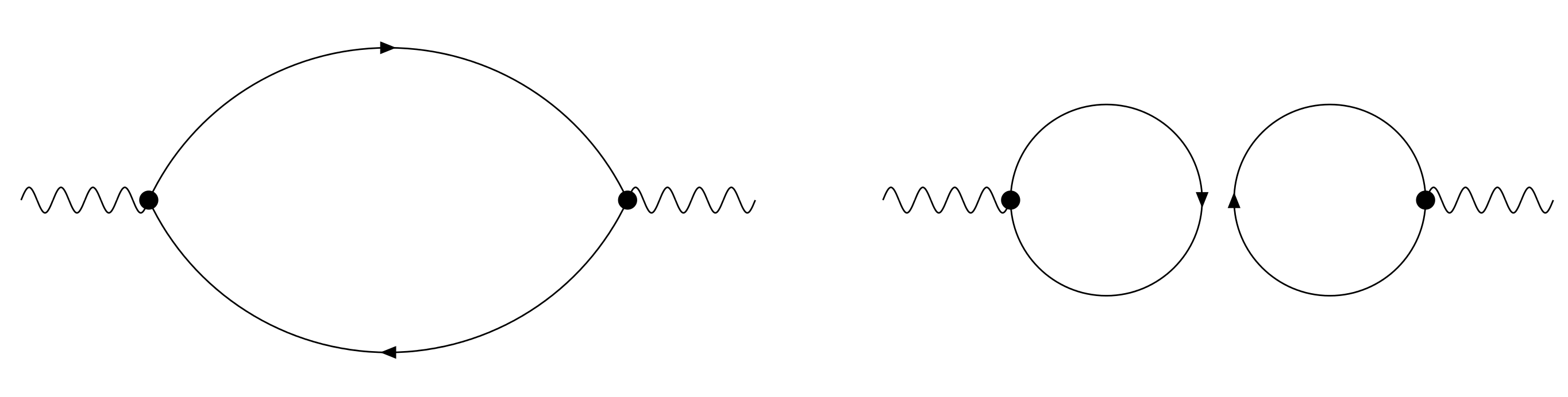
Figure 3: The quark-connected and quark-disconnected diagrams that contribute to the correlator of the electromagnetic current Gluons lines are not shown.

In order to challenge or even surpass the accuracy of the estimates of $a_{\mu}^{\rm hvp}$ obtained using dispersion theory listed in Table 2, lattice calculations must control all sources of statistical and systematic uncertainties at the sub-percent level. This includes the inherent systematic effects that are common to all lattice calculations, i.e. lattice artefacts, finite-volume effects and the dependence on the light quark mass that are discussed in A.5. Since simulations at or very near the physical pion mass are the state of the art, the systematic error associated with the chiral extrapolation is under increasingly good control. Discretisation effects are potentially large for heavy quarks, and since the charm quark makes a small but significant contribution to $a_{\mu}^{\rm hvp}$, the extrapolation to the continuum limit must be sufficiently well controlled. Many quantities computed in lattice QCD, such as hadron masses and decay constants do not receive large finite-volume corrections relative to the typical statistical error, provided that $m_{\pi}L\gtrsim 4$. However, this is only an empirical statement derived from a finite set of quantities, and it is uncertain whether this rule of thumb applies to $a_{\mu}^{\rm hvp}$. At the sub-percent level, isospin breaking effects arising from the mass splitting among the up and down quarks, as well as from their different electric charges cannot be neglected. This represents a major complication, since calculations for $m_{u}\neq m_{d}$ are technically more involved and because QED effects must be incorporated as well [68, 69, 70, 66, 71, 72, 73, 74, 75, 76, 77, 78, 64] (see also the recent review [79]). Finally, there is the issue of quark-disconnected diagrams: after performing the Wick contractions over the quark fields in the vector correlator of Eq. (9) one recovers the two types of diagrams shown in Figure 3. Due to the large inherent level of statistical fluctuations, special noise reduction techniques must be applied in order to determine the contributions from quark-disconnected diagrams with sufficient accuracy. Isospin symmetry implies that, in the low-energy regime, the disconnected contribution to $\hat{\Pi}(Q^{2})$ amounts to $-1/10$ of the connected one [80, 81]. While this estimate for the ratio is essentially confirmed in chiral effective theory at two loops [82], it is necessary to evaluate disconnected contributions directly using actual simulation data if the overall target precision is set below 1%. We postpone a detailed discussion of quark-disconnected diagrams to Section 2.3.

2.2 The infrared regime of $\Pi(Q^{2})$

In this subsection we will discuss the strategies that are employed to determine the subtracted vacuum polarisation $\hat{\Pi}(Q^{2})\equiv 4\pi^{2}(\Pi(Q^{2})-\Pi(0))$ with sufficient accuracy in the low-momentum region. We will focus, in particular, on the determination of the additive renormalisation $\Pi(0)$. Recalling the relation between the vacuum polarisation tensor and $\Pi(Q^{2})$ in Eq. (11) one easily sees that the statistical accuracy of $\Pi(Q^{2})$ deteriorates near $Q^{2}=0$, which makes an accurate determination of $\Pi(0)$ quite difficult. In early calculations of $a_{\mu}^{\rm hvp}$ the value of $\Pi(0)$ was determined by performing fits to $\Pi(Q^{2})$ over the entire accessible range in $Q^{2}$, using some ansatz for the momentum dependence. The disadvantage of such a procedure lies in the fact that the higher statistical accuracy of the data points at larger values of $Q^{2}$ may lead to a systematic bias in the shape of $\Pi(Q^{2})$ in the momentum range from which the convolution integral in Eq. (13) receives its dominant contribution. This issue bears some resemblance to the determination of the proton charge radius from $ep$ scattering data [83, 84].

2.2.1 The “hybrid method”

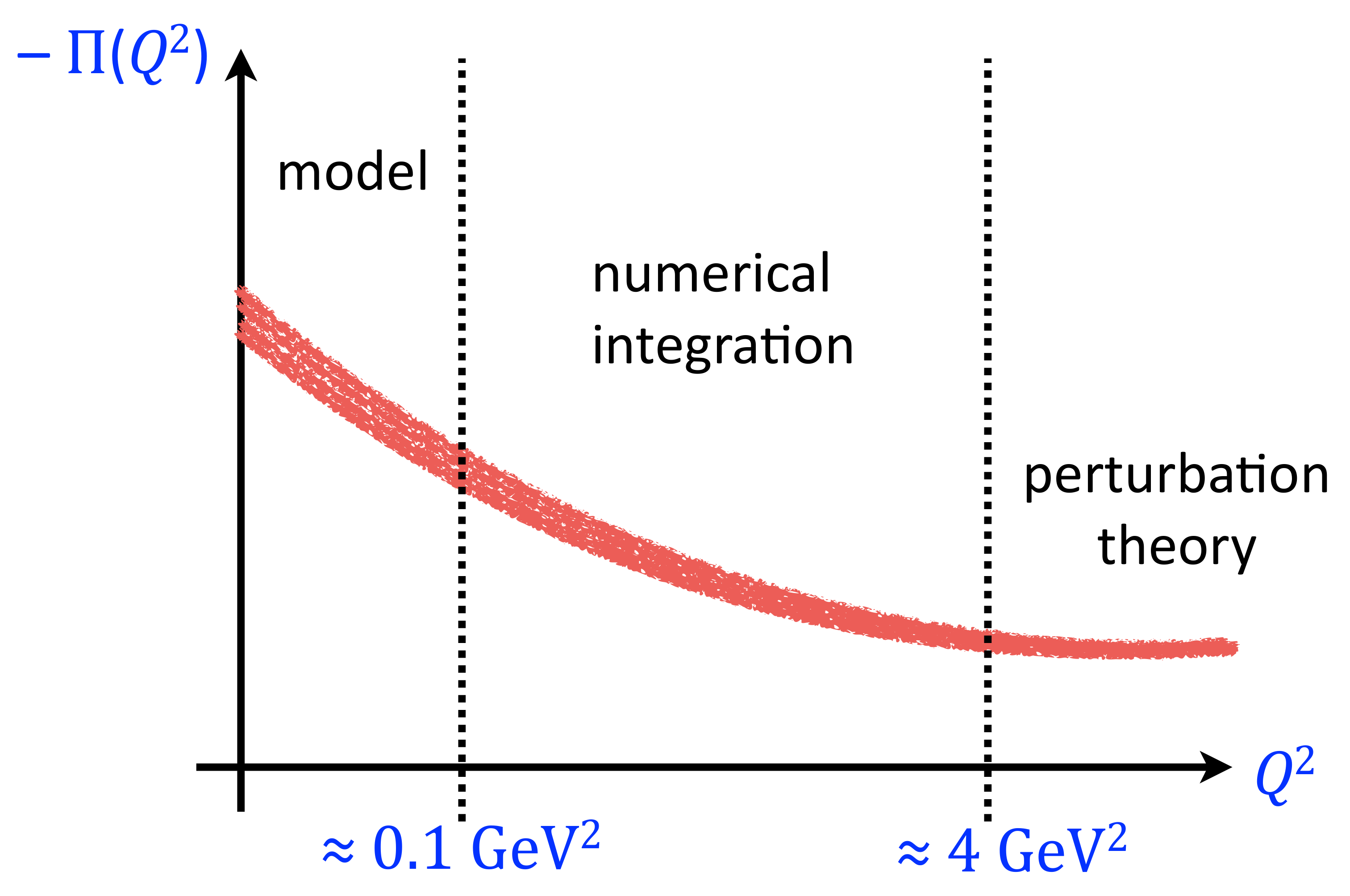
Figure 4: Sketch of the hybrid method introduced in Ref. [85]. The red band denotes the unsubtracted vacuum polarisation $\Pi(Q^{2})$. The model ansatz for fitting lattice data for $\Pi(Q^{2})$ in the low-momentum regime are based on Padé approximants or conformal polynomials.

In Ref. [85] the so-called hybrid method was proposed. Here the accessible $Q^{2}$-interval is divided into three parts, as shown schematically in Figure 4. Fits to the unsubtracted vacuum polarisation $\Pi(Q^{2})$ are restricted to the immediate vicinity of $Q^{2}=0$, i.e. to the interval $0\leq Q^{2}\leq Q_{\rm low}^{2}$. Ideally, the scale $Q_{\rm low}$ should be chosen much smaller than the mass of the lowest vector meson, $m_{\rho}$, in order to avoid any bias arising from the parameterisation of $\Pi(Q^{2})$. A possible ansatz for the $Q^{2}$-behaviour in this regime is provided by the Padé approximant of order $[N,M]$:

$$\Pi_{[N,M]}(Q^{2})=\Pi(0)+\frac{a_{1}Q^{2}+a_{2}Q^{4}\ldots+a_{N}Q^{2N}}{1+b_{1}Q^{2}+b_{2}Q^{4}+\ldots+b_{M}Q^{2M}}.$$ (15)

One expects that Padé approximants of increasingly higher degree eventually converge towards a model-independent description of the data [86], so that a determination of the intercept $\Pi(0)$ and the shape of $\Pi(Q^{2})$ in the low-momentum region is obtained which is free of any bias from data points at larger $Q^{2}$. Alternatively, one may use conformal polynomials [87] in the interval $0\leq Q^{2}\leq Q_{\rm low}^{2}$, i.e.

$$\Pi(Q^{2})=\Pi(0)+\sum_{n=1}^{\infty}\,p_{n}w^{n},\quad w=\frac{1-\sqrt{1+z}}{\sqrt{1+z}},\quad z=Q^{2}/4m_{\pi}^{2}.$$ (16)

Given an estimate for $\Pi(0)$ one can determine $\hat{\Pi}(Q^{2})$ over the entire momentum range and evaluate the convolution integral. In the intermediate momentum range, i.e. in the interval $Q_{\rm low}^{2}\leq Q^{2}\leq Q_{\rm high}^{2}$ the integration of $f(Q^{2})\hat{\Pi}(Q^{2})$ can be performed numerically using, for instance, the trapezoidal rule. Typically $Q_{\rm high}^{2}$ is as large as a few ${\rm{GeV}}^{2}$, and hence one can use perturbation theory to continue the integration above $Q_{\rm high}^{2}$.

Obviously, the success of the hybrid method depends on the availability of statistically accurate data for $Q^{2}\leq Q_{\rm low}^{2}$. In addition, a number of strategies for increasing the number of data points in the low-momentum region have been proposed. These include the use of twisted boundary conditions in Ref. [56] that allow for the realisation of momenta which differ from the usual integer multiples of $2\pi/L$. To this end one imposes spatial periodic boundary conditions on the quark fields up to a phase factor [88, 89, 90]

$$\psi(x+L\hat{k})={\rm{e}}^{i\theta_{k}}\psi(x).$$ (17)

This is equivalent to boosting the spatial momenta in the quark propagator by $\theta_{k}/L$. By a suitable tuning of the phase angle $\theta_{k}$ one can thus access much smaller values of $Q^{2}$ than those which can be realised by the usual Fourier momenta. A potential drawback of this procedure is the modification of the Ward identities of the vacuum polarisation tensor due to twisting [91], yet a recent investigation showed that the effect is numerically insignificant [92].

2.2.2 Time moments

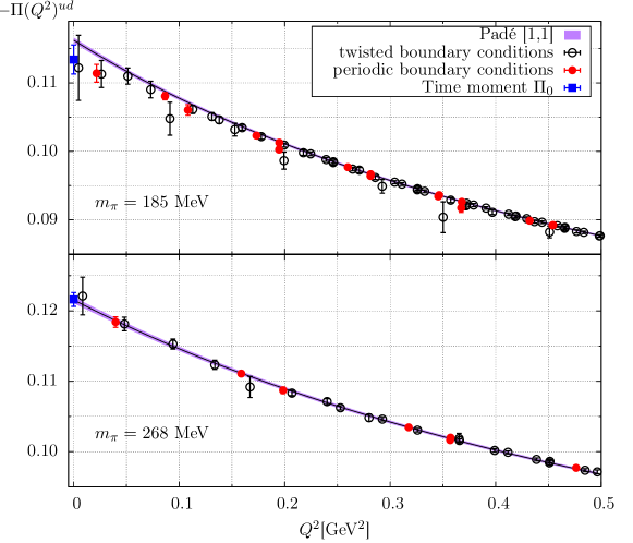
Figure 5: The low-momentum representation of the $u,d$ contributions to $\Pi(Q^{2})$ in terms of a [1,1]-Padé approximation for pion masses of 190 (top) and 270 MeV (bottom), taken from Ref. [62]. The curves represent fits to the data in the interval $0\leq Q^{2}\leq 0.5\,{\rm{GeV}}^{2}$. Blue filled squares indicate the value of $\Pi(0)$ determined from the second time moment.

Another method, proposed in [93], is based on constructing the Padé representation of $\Pi(Q^{2})$ in the interval $0\leq Q^{2}\leq Q_{\rm low}^{2}$ from the time moments of the vector correlator. The starting point is the Taylor expansion

$$\Pi(Q^{2})=\Pi_{0}+\sum_{j=1}^{\infty}\Pi_{j}\,Q^{2j},$$ (18)

with coefficients $\Pi_{0},\Pi_{1},\ldots$. Choosing $Q=(\omega,\boldsymbol{0})$ one finds that the non-vanishing components of the vacuum polarisation tensor are given by (see Eq. (11))

$$\Pi_{kk}(\omega)=\int_{-\infty}^{\infty}dx_{0}\,{\rm{e}}^{i\omega x_{0}}\,\int d^{3}x\left\langle J_{k}(x)J_{k}(0)\right\rangle.$$ (19)

If $G(x_{0})$ denotes the spatially summed vector correlator defined by

$$G(x_{0})\delta_{kl}=-\int d^{3}x\left\langle J_{k}(x)J_{l}(0)\right\rangle,$$ (20)

it is easy to see that the expansion coefficients $\Pi_{j}$ can be expressed in terms of the time moments $G_{2n}$ of $G(x_{0})$, i.e.

$$G_{2n}\equiv\int_{-\infty}^{\infty}dx_{0}\,x_{0}^{2n}\,G(x_{0})=(-1)^{n}\frac{\partial^{2n}}{\partial\omega^{2n}}\left\{\omega^{2}\Pi(\omega^{2})\right\}_{\omega^{2}=0}\,.$$ (21)

The expansion coefficients are then recovered as

$$\Pi_{j}=(-1)^{j+1}\,\frac{G_{2j+2}}{(2j+2)!}.$$ (22)

In particular, the additive renormalisation $\Pi(0)$ is given by the second moment, i.e.

$$\Pi(0)\equiv\Pi_{0}=-\frac{1}{2}G_{2}.$$ (23)

The Taylor coefficients can then be used to construct the Padé approximation of $\Pi(Q^{2})$. For instance, the coefficients $a_{n}$ and $b_{m}$ of the two lowest order Padé approximations (see Eq. (15)) are related to the time moments via

$$\Pi_{[1,1]}: a_{1}=\Pi_{1},\quad b_{1}=-\Pi_{2}/\Pi_{1}$$

$$\Pi_{[2,1]}: a_{1}=\Pi_{1},\quad a_{2}=(\Pi_{2}^{2}-\Pi_{1}\Pi_{3})/\Pi_{2},\quad b_{1}=-\Pi_{3}/\Pi_{1},$$ (24)

while $\Pi(0)=\Pi_{0}$. Figure 5 shows a comparison of the [1,1]-Padé approximation of $\Pi(Q^{2})$ constructed from a fit to the data for $\Pi(Q^{2})$ in the interval $0\leq Q^{2}\leq 0.5\,{\rm{GeV}}^{2}$. The value of the additive renormalisation, $\Pi(0)$, determined from the intercept agrees well with the estimate from the second time moment, $\Pi_{0}=-G_{2}/2$. Note that the results in the figure have been obtained by restricting the electromagnetic current to the quark-connected contributions from up and down quarks, only.

Although the use of time moments avoids the calculation of $\Pi(Q^{2})$ at specific values of $Q^{2}$ as well as the subsequent fit to some ansatz, there are modelling issues that must still be addressed: The fact that the Padé representation is constructed from time moments implies that the same considerations regarding any bias must be applied as in the case where the Padé is determined from fits to $\Pi(Q^{2})$. Secondly, while the moments are obtained by integrating $G(x_{0})$ up to infinitely large Euclidean time separations (see Eq. (21)), the vector correlator is only accessible for a finite number of time slices, due to the finite temporal extent of the lattice and the rapidly decreasing signal-to-noise ratio. Therefore, some degree of modelling is necessary to extrapolate $G(x_{0})$ to infinity. In fact, this issue becomes even more important for the higher moments since the large-$|x_{0}|$ behaviour of the vector correlator is enhanced by increasing powers of $x_{0}^{2}$.

2.2.3 The time-momentum representation

As was first shown in [94] the subtracted vacuum polarisation function admits an integral representation in terms of the spatially summed vector correlator, i.e.

$$\Pi(Q^{2})-\Pi(0)=\frac{1}{Q^{2}}\int_{0}^{\infty}dx_{0}\,G(x_{0})\,\left[Q^{2}x_{0}^{2}-4\sin^{2}\left({\textstyle\frac{1}{2}}Qx_{0}\right)\right].$$ (25)

When inserted into the convolution integral, Eq. (13), one can re-arrange the order of the integrations, leading to the expression

$$a_{\mu}^{\rm hvp}=\left(\frac{\alpha}{\pi}\right)^{2}\int_{0}^{\infty}\,dx_{0}\,w(x_{0})G(x_{0}),$$ (26)

where the kernel function $w(x_{0})$ is given by

$$w(x_{0})=4\pi^{2}\int_{0}^{\infty}\frac{dQ^{2}}{Q^{2}}\,f(Q^{2})\left[Q^{2}x_{0}^{2}-4\sin^{2}\left({\textstyle\frac{1}{2}}Qx_{0}\right)\right],$$ (27)

and $f(Q^{2})$ denotes the momentum-space kernel of Eq. (14).

The time-momentum representation is closely related to the expression for $\hat{\Pi}(Q^{2})$ in terms of time moments. By expanding the kernel $\left\{Q^{2}x_{0}^{2}-4\sin^{2}\left({\textstyle\frac{1}{2}}Qx_{0}\right)\right\}$ in a Taylor series in $Q^{2}$ one recovers the expression for the subtracted vacuum polarisation function in powers of $Q^{2}$ as

$$\Pi(Q^{2})-\Pi(0)=\sum_{k=1}^{\infty}\left\{\frac{(-1)^{k+1}}{(2k+2)!}\int_{-\infty}^{\infty}dx_{0}\,x_{0}^{2k+2}\,G(x_{0})\right\}Q^{2k}.$$ (28)

Here the expression in curly brackets reproduces the time moment $\Pi_{k}$, as can be seen from Eqs. (21) and (22). Thus, the time-momentum representation is equivalent to the exact Taylor series of $\hat{\Pi}(Q^{2})$.

In both methods, the vector correlator must be integrated up to infinite Euclidean time. On a finite lattice with temporal dimension $T$ and periodic boundary conditions the maximum time extension that can be achieved is $T/2$. More importantly, however, the relative statistical precision of the vector correlator declines sharply [95, 96] so that the computed data for $G(x_{0})$ provide only an increasingly inaccurate constraint on the long-distance part of the integrand in Eq. (26). It is customary to split the vector correlator according to

$$G(x_{0})=\left\{\begin{array}[]{ll}G(x_{0})_{\rm data},&x_{0}\leq x_{0}^{\rm{cut}}\\ G(x_{0})_{\rm ext},&x_{0}>x_{0}^{\rm{cut}}\end{array}\right.,$$ (29)

where $x_{0}^{\rm{cut}}\gtrsim 1.5-2$ fm, and the subscript “ext” indicates that the correlator is being extended by a continuous function in $x_{0}$.

For the following discussion it is useful to consider the decomposition of the electromagnetic current into an iso-vector ($I=1$) and an iso-scalar ($I=0$) part, according to

$$J_{\mu}(x)=J_{\mu}^{\rho}(x)+J_{\mu}^{I=0}(x),$$

$$J_{\mu}^{\rho}={\textstyle\frac{1}{2}}(\bar{u}\gamma_{\mu}u-\bar{d}\gamma_{\mu}d),\quad J_{\mu}^{I=0}={\textstyle\frac{1}{6}}(\bar{u}\gamma_{\mu}u+\bar{d}\gamma_{\mu}d-2\bar{s}\gamma_{\mu}s+\ldots),$$ (30)

where we have used the superscript $\rho$ to denote the iso-vector contribution. The associated correlator is defined by

$$G^{\rho\rho}(x_{0})\,\delta_{kl}=-\int d^{3}x\,\left\langle J_{k}^{\rho}(x)J_{l}^{\rho}(0)\right\rangle.$$ (31)

The corresponding isospin decomposition of the vector correlator reads

$$G(x_{0})=G^{\rho\rho}(x_{0})+G(x_{0})^{(I=0)},$$ (32)

and it is important to realise that the iso-vector part $G^{\rho\rho}$ is proportional to the quark-connected light quark contribution $G^{ud}$ defined according to Eq. (206), i.e.

$$G^{\rho\rho}(x_{0})=\frac{9}{10}\,G^{ud}(x_{0}).$$ (33)

Since the spectral function in the iso-scalar channel vanishes below the 3-pion threshold, one expects that $G(x_{0})$ is dominated by the lowest-energy state in the iso-vector channel as $x_{0}\to\infty$. Thus, the simplest ansatz for $G(x_{0})_{\rm ext}$ is a single exponential:

$$G(x_{0})_{\rm ext}=|A_{\rho}|^{2}\,{\rm{e}}^{-m_{\rho}x_{0}},$$ (34)

where $m_{\rho}$ denotes the $\rho$-meson mass and $A_{\rho}$ is the matrix element of the vector current and the vacuum. Obviously, this ansatz ignores the fact that the iso-vector correlator is dominated by the two-pion state as $x_{0}\to\infty$. The starting point for a rigorous treatment of the long-distance regime of $G^{\rho\rho}$ is the observation that the spectrum in a finite volume of spatial dimension $L$ is discrete. The iso-vector correlator is then given by a sum of exponentials

$$G^{\rho\rho}(x_{0},L)=\sum_{n}\,|A_{n}|^{2}\,{\rm{e}}^{-\omega_{n}x_{0}},\quad\omega_{n}=2\sqrt{m_{\pi}^{2}+k^{2}},$$ (35)

where the argument of $G^{\rho\rho}$ explicitly indicates that we work in a finite volume. The sum runs over all energy eigenstates, and $A_{n}$ is the matrix element of the iso-vector current between the $n^{\rm th}$ state and the vacuum. The energies $\omega_{n}$ are related to the scattering momentum $k$ via the Lüscher condition [97, 98]

$$\delta_{1}(k)+\phi(q)=0\;{\rm mod}\;\pi,\quad q=\frac{kL}{2\pi},$$ (36)

where $\delta_{1}$ is the infinite-volume scattering phase shift, and the function $\phi(z)$ is defined by [98]

$$\phi(z)=-\frac{\pi^{3/2}z}{{\cal{Z}}_{00}(1;z^{2})},\quad{\cal{Z}}_{00}(s;z^{2})=\frac{1}{\sqrt{4\pi}}\sum_{\boldsymbol{n}\in{\mathds{Z}}^{3}}\frac{1}{({\boldsymbol{n}}^{2}-z^{2})^{s}}.$$ (37)

Below the inelastic threshold, i.e. for $2m_{\pi}\leq\sqrt{s}\leq 4m_{\pi}$, the amplitudes $A_{n}$ can be expressed in terms of the timelike pion form factor [99] via a Lellouch-Lüscher factor [100]

$$|A_{n}|^{2}=\,\frac{2k^{5}}{3\pi\omega_{n}^{2}}\,\frac{|F_{\pi}(\omega_{n})|^{2}}{q\phi^{\prime}(q)+k\delta_{1}^{\prime}(k)}.$$ (38)

The $p$-wave scattering phase shift can be determined by computing suitable correlation matrices, followed by the projection onto the approximate energy eigenstates via the variational method [101, 102] and solving for Eq. (36) (see Refs. [103, 104, 105, 106, 107, 108, 109, 110, 111, 112, 113, 114, 115]). The matrix elements $A_{n}$ can be determined from ratios of correlators involving the vector current and the linear combination of interpolating operators that represent the $n^{\rm th}$ energy eigenstate [110, 116, 115]. As a side remark we note that the matrix elements $|A_{n}|$ and the associated timelike pion form factor allow for a reliable determination of finite-volume corrections to $a_{\mu}^{\rm hvp}$ (see Section 2.4).

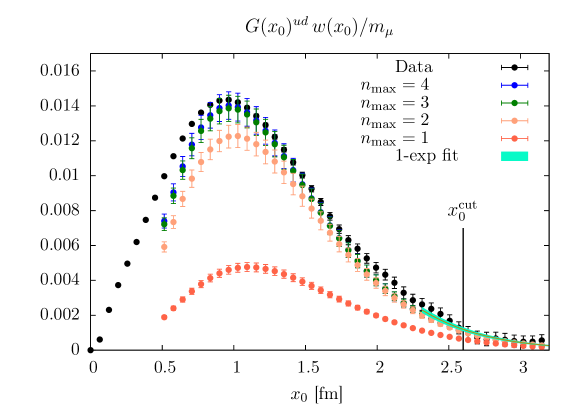
Figure 6: The light quark contribution to the integrand, $w(x_{0})G(x_{0})^{ud}$, in units of $m_{\mu}$, computed for $N_{\rm f}=2+1$ at $m_{\pi}=200$ MeV [117]. Black filled squares represent the direct calculation of the spatially summed vector correlator. The red circles denote the two-pion contribution to the iso-vector correlator $G^{\rho\rho}$, with the remaining coloured points showing the accumulated contributions from the higher excited states. The green band denotes the naive single-exponential ansatz for the extension of $G(x_{0})^{ud}$.

Replacing the infinite sum in Eq. (35) by the sum over a handful of lowest-lying states is an excellent approximation of the iso-vector correlator $G^{\rho\rho}(x_{0},L)$ for $x_{0}\gtrsim 1.5$ fm. Since the iso-scalar contribution to $G(x_{0})$ is sub-dominant, one may replace $G(x_{0})^{(I=0)}$ in Eq. (32) by a single exponential whose fall-off is given by $m_{\omega}\approx m_{\rho}$. In Figure 6 we show a calculation of the light-quark contribution $w(x_{0})\,G^{ud}(x_{0})$ to the integrand in Eq. (26) by CLS/Mainz [117]. It is obvious that the statistical accuracy of the direct calculation (represented by the black points) deteriorates for $x_{0}\gtrsim 2$ fm. By contrast, a much more precise determination of the long-distance regime is obtained through the auxiliary calculation of $G^{\rho\rho}(x_{0},L)$. In particular, one finds that the first four lowest-lying states saturate the correlator for $x_{0}\gtrsim 1.2$ fm. Furthermore, the two-pion contribution, shown in red, is clearly visible and dominates the correlator for distances $x_{0}\gtrsim 3.0$ fm. It is also interesting to note that a naive single exponential, shown by the green band, provides a fairly good description of the tail of the correlator.

A simple method for constraining the large-$x_{0}$ behaviour of $G(x_{0})$ is described in Ref. [61]. On a lattice with temporal and spatial dimensions $T$ and $L$, the correlator $G(x_{0})$ is expected to be dominated by a two-pion state as $x_{0}\to\infty$. Asymptotically, the corresponding correlator $G^{2\pi}(x_{0})$ has the form

$$G^{2\pi}(x_{0})\propto\left({{\rm{e}}}^{-E_{2\pi}x_{0}}+{{\rm{e}}}^{-E_{2\pi}(T-x_{0})}\right).$$ (39)

For the purpose of constraining the long-distance regime of $G(x_{0})$ one may approximate the energy level $E_{2\pi}$ by the energy of two non-interacting pions whose momenta are each given by the smallest non-vanishing value $2\pi/L$, i.e.

$$E_{2\pi}=\sqrt{m_{\pi}^{2}+\left(\frac{2\pi}{L}\right)^{2}}.$$ (40)

Since the iso-vector correlator is a sum of exponentials with positive semi-definite coefficients, it is bounded from below and above according to

$$0\leq G(x_{0})\leq G(x_{0}^{\rm cut})\frac{G^{2\pi}(x_{0})}{G^{2\pi}(x_{0}^{\rm cut})},$$ (41)

since $G(x_{0})$ must fall off faster than $G^{2\pi}(x_{0})$. By truncating the integration interval in Eq. (26) at $x_{0}=x_{0}^{\rm{cut}}$ and inserting the lower and upper bounds in Eq. (41) to evaluate the remainder, one can monitor the resulting upper and lower estimates for $a_{\mu}^{\rm hvp}$ as a function of $x_{0}^{\rm{cut}}$. Figure 7, taken from the calculation by the BMW collaboration [65], shows that the upper and lower bounds agree at $x_{0}^{\rm{cut}}\approx 3.0$ fm, which coincides with the observation by CLS/Mainz [117] that the two-pion states saturates the iso-vector correlator for $x_{0}\gtrsim 3.0$ fm.

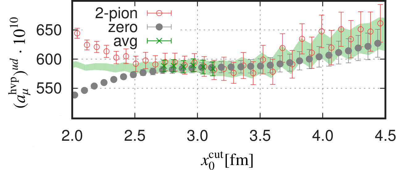
Figure 7: Illustration of the “bounding method” from Ref. [65]. The red and grey data points denote the estimates of the light quark contribution to $a_{\mu}^{\rm hvp}$ obtained by inserting the upper and lower bounds in the evaluation of the convolution integral for $x_{0}>x_{0}^{\rm{cut}}$. Green crosses represent the average of the upper and lower bounds in the regime where they coincide.

We note that the issue how to constrain the deep infrared regime concerns all of the methods discussed above: While the direct calculation of $\Pi(Q^{2})$ raises the question how to describe the low-$Q^{2}$ regime in an unbiased way, one must address the problem of describing the long-distance behaviour of $G(x_{0})$ when employing the time-momentum representation or time moments. Moreover, the issue is intimately linked to the problem of finite-volume effects [62] (see Section 2.4).

2.2.4 Lorentz-covariant coordinate space representation

In the time-momentum representation, Eq. (26), the HVP contribution is the time integral over the spatially summed vector correlator $G(x_{0})$ multiplied by a weight function $w(x_{0})$. As shown in Ref. [118], $a_{\mu}^{\rm hvp}$ can also be expressed in terms of a manifestly Lorentz-covariant integral involving the point-to-point vector correlator $G_{\mu\nu}(x)\equiv\langle J_{\mu}(x)J_{\nu}(0)\rangle$. A particular benefit of this method may be the reduction of the noise-to-signal ratio, especially for the quark-disconnected contribution. The starting point for the derivation is the representation of $a_{\mu}^{\rm hvp}$ in terms of the Adler function $D(Q^{2})$:

$$D(Q^{2})\equiv Q^{2}\frac{d}{dQ^{2}}\,\Pi(Q^{2})=Q^{2}\int_{0}^{\infty}ds\,\frac{\rho(s)}{(s+Q^{2})^{2}}\,,$$ (42)

where the spectral density $\rho(s)$ is related to the $R$-ratio by

$$\rho(s)=\frac{R(s)}{12\pi^{2}},\quad R(s)\equiv\frac{\sigma(e^{+}e^{-}\to\hbox{hadrons})}{4\pi\alpha^{2}/(3s)},$$ (43)

and $a_{\mu}^{\rm hvp}$ is obtained via the convolution integral as [119]

$$a_{\mu}^{\rm hvp}=2\pi^{2}\left(\frac{\alpha}{\pi}\right)^{2}\int_{0}^{1}\frac{dy}{y}(1-y)(2-y)\,D(Q^{2}(y)).$$ (44)

The integration variable $y$ is related to the Euclidean four-momentum $Q$ via

$$y=\frac{2|Q|}{|Q|+\sqrt{4m_{\mu}^{2}+Q^{2}}}\quad\Leftrightarrow\quad Q^{2}=\frac{y^{2}}{1-y}\,m_{\mu}^{2}.$$ (45)

Equivalently, one can express $a_{\mu}^{\rm hvp}$ as an integral over $Q^{2}$ which can be interpreted as a four-dimensional integral over momentum with spherical symmetry [118], i.e.

$$a_{\mu}^{\rm hvp}=\int_{0}^{\infty}dQ^{2}\,D(Q^{2})\,g_{a}(Q^{2})=\frac{1}{\pi^{2}}\int\frac{d^{4}Q}{Q^{2}}\,D(Q^{2})\,g_{a}(Q^{2}),$$ (46)

where

$$g_{a}(Q^{2})=2\alpha^{2}\frac{m_{\mu}^{4}}{|Q|^{6}}\,(y(|Q|))^{4}.$$ (47)

A key observation in Ref. [118] is that the Adler function $D(Q^{2})$ is related to the current-current correlator $G_{\mu\nu}(x)\equiv\langle J_{\mu}(x)J_{\nu}(0)\rangle$ via

$$D(Q^{2})=\frac{1}{3Q^{2}}\left(\delta_{\mu\nu}-\frac{Q_{\mu}Q_{\nu}}{Q^{2}}\right)\int d^{4}x\,G_{\mu\nu}(x)\,{\rm{e}}^{iQ\cdot x}\left(1-{\textstyle\frac{i}{2}}(Q\cdot x)\right),$$ (48)

which, when inserted into Eq. (46), yields the HVP contribution as

$$a_{\mu}^{\rm hvp}=\int d^{4}x\;G_{\mu\nu}(x)\,H_{\mu\nu}(x).$$ (49)

The kernel $H_{\mu\nu}(x)$ is given by

$$H_{\mu\nu}(x)=\frac{1}{3\pi^{2}}\left(1-\frac{x_{\lambda}}{2}\frac{\partial}{\partial x_{\lambda}}\right)\int\frac{d^{4}Q}{(Q^{2})^{2}}\,g_{a}(Q^{2})\,\left(\delta_{\mu\nu}-\frac{Q_{\mu}Q_{\nu}}{Q^{2}}\right)\,{\rm{e}}^{iQ\cdot x},$$ (50)

with $g_{a}(Q^{2})$ specified in Eq. (47). In [118] it was shown that the tensor $H_{\mu\nu}(x)$ can be expressed in terms of weight functions ${\cal{H}}_{1}(|x|)$ and ${\cal{H}}_{2}(|x|)$ that are analytically computable in terms of Bessel functions. Furthermore, one finds that, once the space-time indices of $G_{\mu\nu}$ and $H_{\mu\nu}$ are contracted, the integration over the four-volume becomes a one-dimensional integral over $|x|$.

Another important result of [118] is the Lorentz-covariant expression for the slope of the Adler function and, equivalently, the vacuum polarisation function $\Pi(Q^{2})$, i.e.

$$D^{\prime}(0)=\Pi^{\prime}(0)=\frac{1}{1152}\int d^{4}x\;G_{\mu\nu}(x)\,(x^{2})^{2}\,\left(-\frac{7}{4}\delta_{\mu\nu}+\frac{x_{\mu}x_{\nu}}{x^{2}}\right).$$ (51)

This is the Lorentz-covariant analogue of the relation between the slope $\Pi^{\prime}(0)$ and the time-moment $G_{4}$ (see Eq. (22)):

$$\Pi^{\prime}(0)=\Pi_{1}=\frac{1}{4!}\int_{-\infty}^{\infty}dx_{0}\,G(x_{0})\,x_{0}^{4}.$$ (52)

The advantage of the covariant integral representation of Eq. (49) is that only those space-time points are summed over that contribute to $a_{\mu}^{\rm hvp}$ up to some particular precision. For instance, one may define an effective HVP contribution via

$$(a_{\mu}^{\rm hvp})^{\rm eff}(R)=\int_{|x|<R}d^{4}x\,G_{\mu\nu}(x)\,H_{\mu\nu}(x),$$ (53)

in which the integration domain is truncated to a sphere with radius $R$. The convergence of $(a_{\mu}^{\rm hvp})^{\rm eff}(R)$ towards $a_{\mu}^{\rm hvp}$ can then be studied systematically by increasing the radius $R$. By contrast, in the time-momentum representation (and also when computing $\Pi(Q^{2})$ via Eq. (9)), the vector correlator is summed over the entire spatial volume, even though points very far from the origin barely contribute. This observation also suggests that the estimation of contributions from quark-disconnected diagrams via the covariant formulation may be statistically more precise. First results indicate that this is indeed the case [120].

2.2.5 Other methods for determining $\Pi(0)$

The extensive literature on lattice determinations of $a_{\mu}^{\rm hvp}$ contains further proposals for computing the additive renormalisation $\Pi(0)$.

In Ref. [121] it was noted that the vacuum polarisation $\Pi(Q^{2})$ can be interpreted in terms of magnetic susceptibilities which, in turn, are defined by taking derivatives of the free energy with respect to an external magnetic field. For non-zero values of $Q^{2}$ the vacuum polarisation is obtained from the susceptibility derived from a harmonically varying magnetic field. Moreover, the additive renormalisation $\Pi(0)$ is related to the susceptibility $\chi_{0}$ which characterises the response of the system to applying a homogeneous background field, i.e.

$$\chi_{0}=\Pi(0).$$ (54)

The main conceptual difficulty arises from the fact that taking derivatives with respect to a homogeneous magnetic field is not straightforward, since in a finite volume one has to deal with a non-vanishing magnetic flux. Several methods have been proposed and tested [122, 123] which give mostly consistent results. A pilot study using rooted staggered quarks on coarse lattice spacings shows that this approach yields promising results concerning the overall accuracy [121], yet the method has not been applied in large-scale calculations of $a_{\mu}^{\rm hvp}$ aimed at rivalling the precision of the dispersive method.

A variant of the method that relates $\Pi(0)$ to the time moment $G_{2}$ via $\Pi(0)\equiv\Pi_{0}=-G_{2}/2$ has been proposed in [124]. Here the idea is to apply the second derivative with respect to the momentum directly to the correlation function of the vector current. The momentum derivatives correspond to operator insertions in the correlator, so that $\Pi(0)$ can be computed directly in terms of four-point, three-point and two-point correlation functions. First results obtained at large pion masses indicate that $\Pi(0)$ can be obtained with good statistical precision. The technical challenge of the method consists in isolating the asymptotic behaviour of three- and four-point correlation functions.

2.2.6 Mellin-Barnes representation and time moments

The difficulty to reach small values of the squared Euclidean momentum in lattice simulations has been the motivation for several recent analyses, aimed at providing an alternative representation of $a_{\mu}^{\rm hvp}$ in terms of quantities that can easily be computed in lattice calculations [125, 126, 127]. The starting point is the Mellin-Barnes representation of the hadronic vacuum polarisation

$$a_{\mu}^{\rm hvp}=\left(\frac{\alpha}{\pi}\right)^{2}\frac{1}{2\pi i}\int_{c-i\infty}^{c+i\infty}\,{\cal{F}}(s){\cal{M}}(s),$$ (55)

where the exact kernel function ${\cal{F}}(s)$ is given in terms of Euler $\Gamma$-functions

$${\cal{F}}(s)=-\Gamma(3-2s)\Gamma(-3+s)\Gamma(1+s),$$ (56)

and ${\cal{M}}(s)$ denotes the Mellin transform of the hadronic spectral function

$${\cal{M}}(s)=\int_{t_{0}=4m_{\pi}^{2}}^{\infty}\frac{dt}{t}\,\left(\frac{t}{t_{0}}\right)^{s-1}\frac{1}{\pi}\,{\rm Im}\hat{\Pi}(t).$$ (57)

As proposed in [125] one can perform a low-momentum expansion of the kernel function ${\cal{F}}(s)$ by calculating its residues and poles. This yields the expansion of $a_{\mu}^{\rm hvp}$ in terms of the Mellin moments [126, 128]

$$a_{\mu}^{\rm hvp} = \left(\frac{\alpha}{\pi}\right)^{2}\frac{m_{\mu}^{2}}{t_{0}}\left\{\frac{1}{3}{\cal{M}}(0)+\frac{m_{\mu}^{2}}{t_{0}}\left[\left(\frac{25}{12}-\ln\frac{t_{0}}{m_{\mu}^{2}}\right){\cal{M}}(-1)+\widetilde{\cal{M}}(-1)\right]\right.$$ (58)

$$+\left(\frac{m_{\mu}^{2}}{t_{0}}\right)^{2}\left[\left(\frac{97}{10}-6\ln\frac{t_{0}}{m_{\mu}^{2}}\right){\cal{M}}(-2)+6\widetilde{\cal{M}}(-2)\right]$$

$$+\left(\frac{m_{\mu}^{2}}{t_{0}}\right)^{3}\left[\left(\frac{208}{5}-28\ln\frac{t_{0}}{m_{\mu}^{2}}\right){\cal{M}}(-3)+28\widetilde{\cal{M}}(-3)\right]+\,{\rm{O}}\left(\left(m_{\mu}^{2}/t_{0}\right)^{4}\right)\Bigg{\}}.$$

The key observation is that the moments ${\cal{M}}(-n)$ are related to the derivatives of $\hat{\Pi}(Q^{2})$ which can be computed on the lattice from time moments, i.e.

$${\cal{M}}(-n)\equiv\int_{0}^{\infty}\frac{dt}{t}\,\left(\frac{t_{0}}{t}\right)^{n+1}\frac{1}{\pi}\,{\rm Im}\,\hat{\Pi}(t)=\frac{(-1)^{n+1}}{(n+1)!}\,t_{0}^{n+1}\left.\frac{\partial^{n+1}}{(\partial Q^{2})^{n+1}}\,\hat{\Pi}(Q^{2})\right|_{Q^{2}=0}.$$ (59)

In other words, the determination of the first few terms in the Taylor expansion of $\hat{\Pi}(Q^{2})$ yields the Mellin transform of the spectral function at negative integer argument [126]. Computing the slope $\Pi_{1}$ and the curvature $\Pi_{2}$ via Eq. (22) should already provide a precise estimate of $a_{\mu}^{\rm hvp}$ due to the good convergence property of the expansion in terms of the Mellin moments. When applied to phenomenological models for $\hat{\Pi}(Q^{2})$ such as the one described in [94], one finds that the expansion up to ${\rm{O}}((m_{\mu}^{2}/t_{0})^{2})$ already provides an excellent approximation [125, 126].

The expression in Eq. (58) also contains the first derivatives of ${\cal{M}}(s)$, defined by

$$\widetilde{\cal{M}}(s)\equiv-\frac{d}{ds}{\cal{M}}(s)=\int_{0}^{\infty}\frac{dt}{t}\,\left(\frac{t_{0}}{t}\right)^{1-s}\ln\frac{t_{0}}{t}\frac{1}{\pi}\,{\rm Im}\hat{\Pi}(t).$$ (60)

Their determination is, however, more involved and requires the evaluation of an integral over the subtracted vacuum polarisation $\Pi(Q^{2})$ weighted by inverse powers of $Q^{2}$. Lattice calculations of $\widetilde{\cal{M}}(s)$ will thus be confronted with similar problems as those encountered for the integral representation of Eq. (13), but for a convolution function which is not as strongly peaked at low momenta as $f(Q^{2})$. Concrete proposals for the determination of the log-weighted moments $\widetilde{\cal{M}}(s)$ from lattice data are described in [127].

In Ref. [127] the Mellin moments were determined using experimental data for $e^{+}e^{-}\to\hbox{hadrons}$, and the resulting values can be used to infer the Taylor coefficients $\Pi_{1}$ and $\Pi_{2}$ which can be directly confronted with lattice calculations. We will present a more detailed discussion in Section 2.8. Moreover, in Ref. [128] the Mellin-Barnes technique was advocated as a viable method to derive a highly precise estimate for $a_{\mu}^{\rm hvp}$, using the Taylor coefficients of $\hat{\Pi}(Q^{2})$ determined either in lattice QCD or from the experimental spectral function.

2.2.7 QCD sum rules and the slope of $\Pi(Q^{2})$.

Lattice QCD also plays a central role in an approach that combines QCD sum rules with lattice calculation of the slope of the vacuum polarisation function $\Pi(Q^{2})$ at $Q^{2}=0$ (i.e. the Taylor coefficient $\Pi_{1}$) as well as experimental data for the hadronic cross section data [129, 130]. The resulting expression for $a_{\mu}^{\rm hvp}$ ensures that the latter contribute only a small part to the overall result, making experimental uncertainties quite irrelevant. It starts with the observation that the QED kernel function $\hat{K}(s)$ in Eq. (6) varies only slowly with $s$ [4]. One may therefore approximate it with a meromorphic function $\hat{K}_{1}(s)$ in the low-energy region [129], e.g.

$$\frac{\hat{K}(s)}{s^{2}}\;\longrightarrow\;\frac{\hat{K}_{1}(s)}{s^{2}}=\frac{\hat{c}_{-2}}{s^{2}}+\hat{c}_{0}+\hat{c}_{1}s,\quad m_{\pi^{0}}^{2}\leq s<s_{0},$$ (61)

where $s_{0}\approx 4\,{{\rm{GeV}}}^{2}$ delineates the low-energy from the perturbative region. The coefficients $\hat{c}_{-2},\hat{c}_{0}$ and $\hat{c}_{1}$ may be determined by requiring

$$\int_{m_{\pi^{0}}^{2}}^{s_{0}}\,\hat{K}(s)\,s^{n-2}\,ds=\int_{m_{\pi^{0}}^{2}}^{s_{0}}\,\hat{K}_{1}(s)\,s^{n-2}\,ds,$$ (62)

for suitably chosen integers $n$. As shown in [130] the sum of the contributions from up, down and strange quarks to $a_{\mu}^{\rm hvp}$ can be separated into four terms:

$$(a_{\mu}^{\rm hvp})^{uds}=a_{\mu}^{\rm SR}+a_{\mu}^{\rm Lat}+a_{\mu}^{\rm Exp}+a_{\mu}^{\rm Pert},$$ (63)

where

$$a_{\mu}^{\rm SR}=\left(\frac{\alpha m_{\mu}}{3\pi}\right)^{2}6{\pi}i\oint_{|s|=s_{0}}ds\,\frac{\hat{K}_{1}(s)}{s^{2}}\,\Pi(s),\quad a_{\mu}^{\rm Lat}=\left(\frac{\alpha m_{\mu}}{3\pi}\right)^{2}12\pi^{2}\,\hat{c}_{-2}\,\Pi_{1},$$ (64)

$$a_{\mu}^{\rm Exp}=\left(\frac{\alpha m_{\mu}}{3\pi}\right)^{2}\int_{4m_{\pi}^{2}}^{s_{0}}ds\frac{\hat{K}(s)-\hat{K}_{1}(s)}{s^{2}}\,R(s)^{\rm data},\quad a_{\mu}^{\rm Pert}=\left(\frac{\alpha m_{\mu}}{3\pi}\right)^{2}\int_{s_{0}}^{\infty}ds\frac{\hat{K}(s)}{s^{2}}\,R(s)^{\rm pQCD}.$$

The integral that appears in the expression for the low-energy contribution $a_{\mu}^{\rm SR}$ can be evaluated using QCD sum rules [130]. While $a_{\mu}^{\rm Exp}$ must be determined using experimental data for the hadronic cross section ratio $R(s)$, the influence of experimental uncertainties is greatly diminished relative to the standard dispersive approach, since $R(s)$ is multiplied by the difference of kernel functions, $\hat{K}(s)-\hat{K}_{2}(s)$, in the integrand. By far the largest contribution to $a_{\mu}^{\rm hvp}$ comes from the term $a_{\mu}^{\rm Lat}$, which contains the slope of $\Pi(s)$ at $s=0$, a quantity that can be obtained in lattice QCD, either from the Padé approximation of the vacuum polarisation function or from time moments. Without going into further detail concerning the evaluation of $a_{\mu}^{\rm SR},a_{\mu}^{\rm Exp}$ and $a_{\mu}^{\rm Pert}$, we refer to Ref. [130] and simply quote the final result as

$$(a_{\mu}^{\rm hvp})^{uds}=\left\{(183.2\pm 2.1)+\left(\frac{\alpha m_{\mu}}{3\pi}\right)^{2}\,12\pi^{2}\,\hat{c}_{-2}\,\Pi_{1}\right\}\cdot 10^{-10}.$$ (65)

After inserting the numerical value for $\hat{c}_{-2}$ determined in [130], i.e. $m_{\mu}^{2}\,\hat{c}_{-2}/3=2.36\cdot 10^{-3}\,{{\rm{GeV}}}^{2}$, one obtains

$$(a_{\mu}^{\rm hvp})^{uds}=\left\{(183.2\pm 2.1)+5027\,\left(\Pi_{1}\,[{{\rm{GeV}}}^{-2}]\right)\,\right\}\cdot 10^{-10},$$ (66)

which is easily converted into a estimate for the hadronic vacuum polarisation, by providing a lattice result for the Taylor coefficient $\Pi_{1}$ in units of ${{\rm{GeV}}}^{-2}$. The contribution from the charm quark must also be added before confronting this method with results from the standard dispersive approach, direct determinations of $a_{\mu}^{\rm hvp}$ in lattice QCD and from the approach based on Mellin-Barnes moments.

2.3 Quark-disconnected diagrams

The correlator of the electromagnetic current contains both quark-connected and quark-disconnected contributions, as depicted in Figure 3. Despite the fact that the latter occur frequently in lattice calculations of a variety of hadronic observables involving flavour-singlet contributions, they have often been ignored for technical reasons related to the large level of statistical noise encountered when the standard techniques for computing quark propagators are employed. Obviously, neglecting this class of diagrams amounts to an uncontrolled approximation, and their inclusion is indispensable if one strives for sub-percent accuracy. For concreteness, we consider the electromagnetic current of Eq. (10), which we write as

$$J_{\mu}(x)=\sum_{f=u,d,s,\ldots}{\cal{Q}}_{f}\,\overline{\psi}_{f}(x)\gamma_{\mu}\psi_{f}(x),$$ (67)

where ${\cal{Q}}_{f}$ denotes the electric charge of quark flavour $f$. After inserting the current into the correlation function and performing the Wick contractions, one obtains

$$\left\langle J_{\mu}(x)J_{\nu}(y)\right\rangle = \phantom{+}\sum_{f}{\cal{Q}}_{f}^{2}\left\langle{\rm Tr\,}\left\{\gamma_{\nu}\gamma_{5}S^{f}(x,y)^{\dagger}\gamma_{\mu}\gamma_{5}S^{f}(x,y)\right\}\right\rangle$$ (68)

$$+\sum_{f,f^{\prime}}{\cal{Q}}_{f}{\cal{Q}}_{f^{\prime}}\left\langle{\rm Tr\,}\left\{\gamma_{\mu}S^{f}(x,x)\right\}\,{\rm Tr\,}\left\{\gamma_{\nu}S^{f^{\prime}}(y,y)\right\}\right\rangle,$$

where $S^{f}$ denotes the quark propagator of flavour $f$, and the second line corresponds to the diagram depicted on the right in Figure 3.

The standard technique for computing the quark propagator $S(x,y)$ amounts to fixing the coordinate $y$ (i.e. the source point) and inverting the lattice Dirac operator $D$, by solving the linear system

$$\sum_{z}D(x,z)\,\phi(z)=\delta_{xy}\quad\Rightarrow\quad\phi(x)=\sum_{z}D^{-1}(x,z)\,\delta_{zy}=D^{-1}(x,y)\equiv S(x,y).$$ (69)

The solution $S(x,y)$ is interpreted as the “point-to-all” propagator, starting from the (fixed) point $y$ to any space-time point $x$ on the lattice. Let us now consider the spatially summed vector correlator $G(x_{0})$, which plays a central role for determining the vacuum polarisation using the time-momentum representation or time moments. Its connected part is easily obtained from the point-to-all propagator via

$$G_{\rm con}(x_{0})=-\frac{a^{3}}{3}\sum_{k=1}^{3}\sum_{f}{\cal{Q}}_{f}^{2}\sum_{\boldsymbol{x}}\left\langle{\rm Tr\,}\left\{\gamma_{k}\gamma_{5}S^{f}(x,0)^{\dagger}\gamma_{k}\gamma_{5}S^{f}(x,0)\right\}\right\rangle,$$ (70)

where we have explicitly chosen $y=0$. The disconnected part of $G(x_{0})$ involves the quantity

$$\Delta^{f}(x_{0})\equiv a^{3}\sum_{\boldsymbol{x}}{\rm Tr\,}\left\{\gamma_{k}S^{f}(x,x)\right\},\quad f=ud,s.$$ (71)

In order to sum over $\boldsymbol{x}$ one has to solve the linear system in Eq. (69) for every spatial coordinate $\boldsymbol{x}$ and repeat this for every timeslice $x_{0}$ to obtain $\Delta^{f}(x_{0})$. Thereby the numerical effort is increased by a factor proportional to the 4-volume of the lattice, which is of order $10^{7}$. This is prohibitively costly, and one usually resorts to stochastic techniques in order to compute the “all-to-all” propagator $S(x,y)$ in which the source point $y$ runs over all points of the lattice. To this end one generalises Eq. (69) according to

$$\sum_{z}\,D(y,z)\phi^{(r)}(z)=\eta^{(r)}(y),\quad r=1,\ldots,N_{\rm r},$$ (72)

where $\eta^{(r)}(y)$ is a random noise vector which satisfies

$$\langle\langle\eta(x)\,\eta^{\dagger}(y)\rangle\rangle\equiv\lim_{N_{\rm r}\to\infty}\frac{1}{N_{\rm r}}\sum_{r=1}^{N_{\rm r}}\eta^{(r)}(x)\,\eta^{(r)}(y)^{\dagger}=\delta_{xy}.$$ (73)

By $\langle\langle\cdots\rangle\rangle$ one denotes the stochastic average over a sample of $N_{\rm r}$ random noise vectors. A few lines of straightforward algebra show that the solution of Eq. (73), i.e.

$$\phi^{(r)}(x)=\sum_{y}S^{f}(x,y)\,\eta^{(r)}(y),$$ (74)

yields $\Delta^{f}(x_{0})$ via the stochastic average involving the original noise vector $\eta^{(r)}$

$$\Delta^{f}(x_{0})=a^{3}\sum_{\boldsymbol{x}}\lim_{N_{\rm r}\to\infty}\frac{1}{N_{\rm r}}\sum_{r=1}^{N_{\rm r}}\,{\rm Tr}\,\left\{\eta^{(r)}(x)^{\dagger}\gamma_{k}\phi^{(r)}(x)\right\}.$$ (75)

We now return to the spatially summed vector correlator $G(x_{0})$ which is the main quantity for the determination of $a_{\mu}^{\rm hvp}$ based either on the time-momentum representation or time moments. We restrict the discussion to the case of the $u,d,s$ quarks, and hence the current components with $\mu=k=1,2,3$ are given by

$$J_{k}={\textstyle\frac{2}{3}}\overline{u}\gamma_{k}u-{\textstyle\frac{1}{3}}\overline{d}\gamma_{k}d-{\textstyle\frac{1}{3}}\overline{s}\gamma_{k}s.$$ (76)

Furthermore, we ignore isospin breaking and set $m_{u}=m_{d}$. The correlator then assumes the form

$$G(x_{0}) = G_{\rm con}^{ud}(x_{0})+G_{\rm con}^{s}(x_{0})-G_{\rm disc}(x_{0}),$$ (77)

$$G_{\rm disc}(x_{0}) = G_{\rm disc}^{ud}(x_{0})+G_{\rm disc}^{s}(x_{0})-2G_{\rm disc}^{ud,s}(x_{0}).$$ (78)

Here we have made the distinction between quark-connected and -disconnected contributions explicit by using the the subscripts “con” and “disc”, while the superscripts indicate whether the contribution involves only light $(ud)$, strange $(s)$ or both $(ud,s)$ quark flavours (for the definition of the connected single-flavour contribution $G^{f}(x_{0})$, see Eq. (206)). In Ref. [131] it was shown that $G_{\rm disc}(x_{0})$ factorises according to

$$G_{\rm disc}(x_{0})=-\frac{1}{9}\left\langle\left(\Delta^{ud}(x_{0})-\Delta^{s}(x_{0})\right)\left(\Delta^{ud}(0)-\Delta^{s}(0)\right)\right\rangle.$$ (79)

It is now important to realise that the stochastic noise in the evaluation of the disconnected part largely cancels in the difference $(\Delta^{ud}-\Delta^{s})$, provided that the same noise vectors $\eta^{(r)}$ are used to compute the individual estimates for $\Delta^{ud}$ and $\Delta^{s}$. In refs. [131, 132] it was demonstrated that this is indeed the case and that the gain in statistical precision amounts to almost two orders of magnitude.

There are several refinements of the method, designed to suppress the intrinsic stochastic noise. One is based on the hopping parameter expansion (HPE) of the quark propagator: The Wilson-Dirac operator can be expressed as a sum of two terms, one of which is diagonal in coordinate space, while the other one, the hopping term $H$, encodes the nearest-neighbour interactions

$$D_{\rm w}=\frac{1}{2\kappa}\mathbb{1}-\frac{1}{2}H.$$ (80)

The hopping parameter $\kappa$ is related to the bare quark mass of flavour $f$, $m_{f}$, via

$$\kappa=\frac{1}{2am_{f}+8}.$$ (81)

With these definitions one can express the quark propagator as [133, 134]

$$S(x,y)=2\kappa\sum_{k=0}^{N-1}\,(\kappa H)^{k}+(\kappa H)^{N}D_{\rm w}^{-1}(x,y).$$ (82)

When $D_{\rm w}^{-1}$ is computed using the noise sources as described above, the stochastic noise is further suppressed by a factor $\kappa^{N}$, where $N$ denotes the order of the HPE. The factors $(\kappa H)^{k}$, on the other hand, contain only products of the hopping matrix $H$ and are cheap to evaluate. The HPE can also be adapted to the case of ${\rm{O}}(a)$ improved Wilson fermions [135, 136].

Another method for achieving stochastic noise cancellation makes use of the spectral decomposition of the quark propagator in terms of eigenvectors of the lattice Dirac operator [137, 138]

$$S(x,y)=\sum_{k=1}^{N_{\rm ev}}\frac{v_{k}(x)\otimes v_{k}(y)^{\dagger}}{\lambda_{k}}+S_{\perp}(x,y)$$ (83)

where the sum runs over the $N_{\rm ev}$ lowest eigenmodes $v_{k}(x)$ of the Dirac operator with eigenvalue $\lambda_{k}$. Stochastic sources are only applied in the calculation of $S_{\perp}(x,y)$, which is the propagator restricted to the orthogonal complement of the subspace spanned by the low modes. If one chooses $N_{\rm ev}$ large enough, so that $\lambda_{N_{\rm{ev}}}\simeq m_{s}$ then the stochastic noise in the calculation of $\Delta^{ud}$ will be suppressed by a factor of ${\rm{O}}(m_{s}^{-1})$, and the signal for $G_{\rm disc}(x_{0})$ will be dominated by the low-mode contribution [58].

Several methods have been developed and tested in order to minimise the stochastic noise in the calculation of the individual flavour contribution $\Delta^{f}$, such as the application of suitable “dilution schemes” [139, 137] which improve the convergence towards the right-hand-side of Eq. (73). Furthermore it was found that the use of four-dimensional random noise vectors, either at fixed momentum [121] or in combination with hierarchical probing [140, 141] is particularly efficient in suppressing stochastic noise.

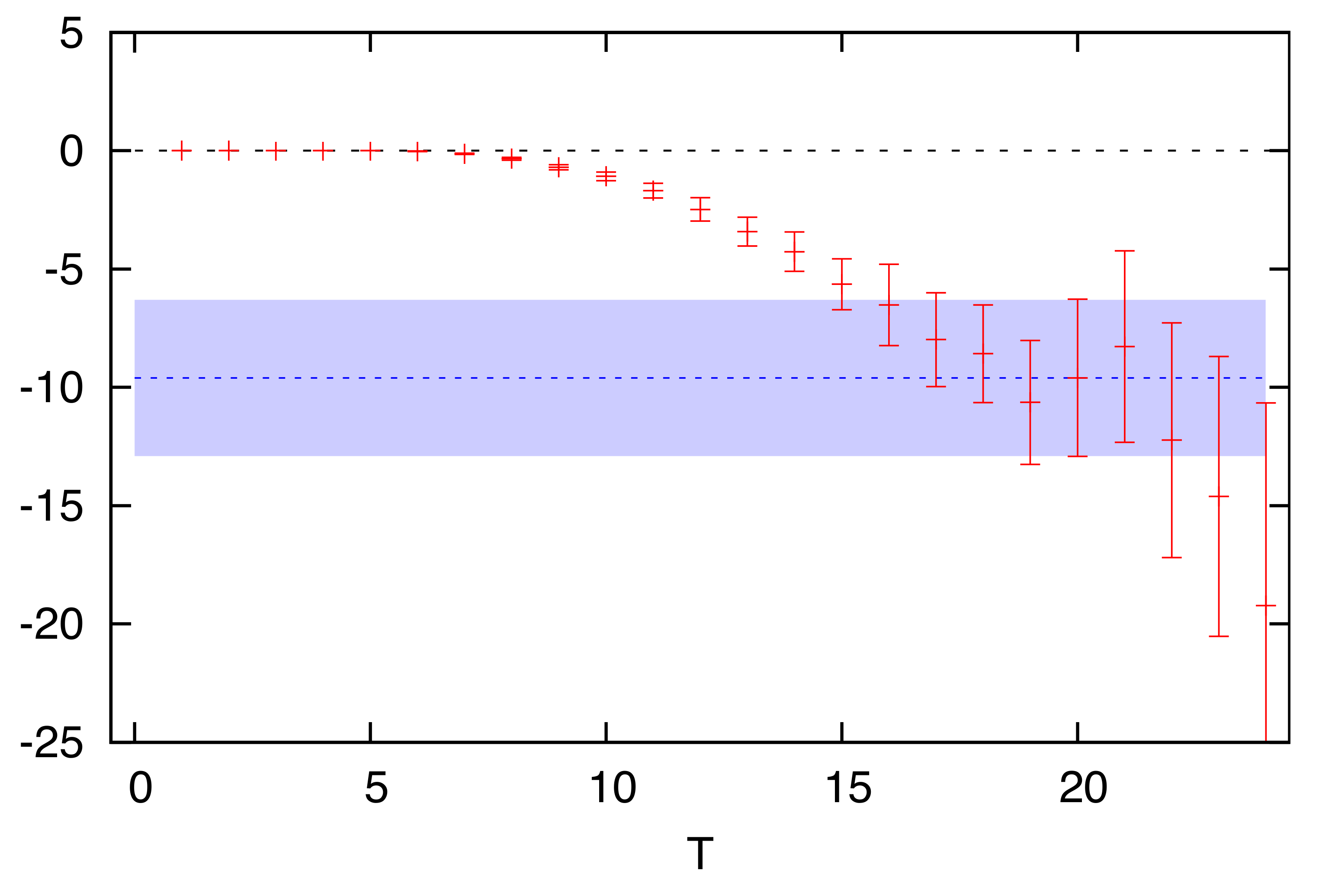
Figure 8: The effective disconnected contribution $(a_{\mu}^{\rm hvp})_{\rm disc}^{\rm eff}(T)$ to the hadronic vacuum polarisation (see Eq. (84)), as computed in [58] plotted versus $T$ in units of $10^{-10}$. The blue band denotes the value at $T=20$.

We will now discuss three specific calculations [58, 62, 61] of the quark-disconnected contribution which are all based on the time-momentum representation. The RBC/UKQCD Collaboration [58] have employed the spectral decomposition of Eq. (83) to compute the disconnected part $G_{\rm disc}(x_{0})$ on gauge ensembles generated using domain wall fermions at the physical pion mass and a lattice spacing of $0.114\,{\rm{fm}}$. In order to quantify the contribution from quark-disconnected diagrams, defined by

$$(a_{\mu}^{\rm hvp})_{\rm disc}=\left(\frac{\alpha}{\pi}\right)^{2}\int_{0}^{\infty}dx_{0}\,(-G_{\rm disc}(x_{0}))\,w(x_{0}),$$ (84)

with $w(x_{0})$ given in Eq. (27), one may consider the effective disconnected contribution

$$(a_{\mu}^{\rm hvp})_{\rm disc}^{\rm eff}(T)\equiv\left(\frac{\alpha}{\pi}\right)^{2}\int_{0}^{T}\,(-G_{\rm disc}(x_{0}))\,w(x_{0}).$$ (85)

As $T\to\infty$ this quantity converges towards $(a_{\mu}^{\rm hvp})_{\rm disc}$. A plateau in a plot of $(a_{\mu}^{\rm hvp})_{\rm disc}^{\rm eff}(T)$ versus $T$ would signal that the sum in Eq. (84) is saturated. As indicated in Figure 8, RBC/UKQCD find that the asymptotic value is reached for $T/a\gtrsim 17$, and the resulting estimate for the quark-disconnected contribution is [58]

$$(a_{\mu}^{\rm hvp})_{\rm disc}=-(9.6\pm 3.3\pm 2.3)\cdot 10^{-10}.$$ (86)

Here the first error is statistical, and the second is an estimate of systematic effects such as discretisation and finite-volume effects.

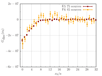
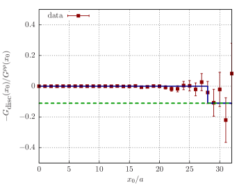
Figure 9: Left: the disconnected contribution $G_{\rm{disc}}$ in two-flavour QCD at pion masses of $440\,{\rm{MeV}}$ (red squares) and $310\,{\rm{MeV}}$ (yellow squares) [62]. Right: the ratio defined in Eq. (92) at $m_{\pi}=440\,{\rm{MeV}}$. The data are compatible with Eq. (92) which is represented by the blue line.

Another determination of the disconnected contribution was performed by CLS/Mainz [62], using two flavours of ${\rm{O}}(a)$ improved Wilson fermions at pion masses of 440 and $310\,{\rm{MeV}}$ and a lattice spacing of $a=0.066\,{\rm{fm}}$. Here the disconnected part was computed employing stochastic noise cancellation as described above. In Refs. [131, 62] the Mainz group describes how an upper bound on the magnitude of the disconnected contribution can be derived. Recalling the isospin decomposition of the vector correlator in Eq. (32), i.e. $G(x_{0})=G^{\rho\rho}(x_{0})+G(x_{0})^{(I=0)}$, one can identify the iso-vector and iso-scalar contributions as

$$G^{\rho\rho}(x_{0}) = \frac{9}{10}G^{ud}_{\rm con}(x_{0}),$$

$$G^{(I=0)}(x_{0}) = \frac{1}{10}G^{ud}_{\rm con}(x_{0})+G^{s}_{\rm con}(x_{0})-G_{\rm disc}(x_{0}).$$ (87)

Using Eq. (77) one can then derive the relation

$$-\frac{G_{\rm disc}(x_{0})}{G^{\rho\rho}(x_{0})}=\frac{G(x_{0})-G^{\rho\rho}(x_{0})}{G^{\rho\rho}(x_{0})}-\frac{1}{9}\left(1+9\frac{G^{s}_{\rm con}(x_{0})}{G^{\rho\rho}(x_{0})}\right).$$ (88)

Since the iso-scalar spectral function vanishes below the three-pion threshold, the long-distance behaviour of the iso-scalar correlator is given by $G^{(I=0)}(x_{0})\sim{\rm{e}}^{-3m_{\pi}x_{0}}$. According to Eq. (87) this implies

$$G_{\rm disc}(x_{0}) = \left({\frac{1}{10}}G^{ud}_{\rm con}(x_{0})+G^{s}_{\rm con}(x_{0})\right)\cdot(1+{\rm{O}}({\rm{e}}^{-m_{\pi}x_{0}})),$$ (89)

$$G(x_{0}) = G^{\rho\rho}(x_{0})\cdot(1+{\rm{O}}({\rm{e}}^{-m_{\pi}x_{0}}))$$ (90)

in the deep infrared. In this way one can derive the asymptotic behaviour of the ratio in Eq. (88) in the long-distance regime as

$$-\frac{G_{\rm disc}(x_{0})}{G^{\rho\rho}(x_{0})}\stackrel{{\scriptstyle x_{0}\to\infty}}{{\longrightarrow}}-\frac{1}{9},$$ (91)

where it is taken into account that $G^{s}_{\rm con}(x_{0})$ drops off faster than $G^{\rho\rho}(x_{0})$ due to the heavier mass of the strange quark.

Data for the correlator ratio $-{G_{\rm disc}}/{G^{\rho\rho}}$ are shown in the right-hand panel of Figure 9 [62]. While there is no visible trend that the ratio approaches the asymptotic value of $-1/9$ for $x_{0}/a\lesssim 26$ or $x_{0}\lesssim 1.7$ fm, one may still derive an upper bound on the magnitude of the disconnected contribution: To this end one assumes that the ratio drops to $-1/9$ at $x_{0}=x_{0}^{\ast}$, which marks the timeslice where the precision is insufficient to distinguish between zero and the expected asymptotic value. In other words, $x_{0}^{\ast}$ is chosen such that the data are statistically compatible with

$$-\frac{G_{\rm disc}(x_{0})}{G^{\rho\rho}(x_{0})}=\left\{\begin{array}[]{cl}0,&x_{0}\leq x_{0}^{\ast},\\ -1/9,&x_{0}>x_{0}^{\ast}\end{array}\right.$$ (92)

One can now define the relative size of the connected and disconnected contributions to $a_{\mu}^{\rm hvp}$ via

$$\Delta a_{\mu}^{\rm hvp}\equiv-\frac{(a_{\mu}^{\rm hvp})_{\rm disc}}{(a_{\mu}^{\rm hvp})_{\rm con}}>0,$$ (93)

with $(a_{\mu}^{\rm hvp})_{\rm disc}$ defined in Eq. (84). After inserting Eq. (92) one obtains the upper bound on the magnitude of $(a_{\mu}^{\rm hvp})_{\rm disc}$ as

$$\left|(a_{\mu}^{\rm hvp})_{\rm disc}\right|^{\rm(max)}=\frac{1}{10}\left(\frac{\alpha}{\pi}\right)^{2}\int_{x_{0}^{\ast}}^{\infty}dx_{0}\,G^{ud}_{\rm con}(x_{0}))\,w(x_{0}).$$ (94)

In their two-flavour calculation [62] CLS/Mainz find that $\Delta a_{\mu}^{\rm hvp}$ is less than 1% for a pion mass of 440 MeV but that the magnitude increases to 2% for $m_{\pi}=310$ MeV, which is the estimate quoted in Table 3 and represented by the red band in Figure 11.

Not only the fraction of the disconnected contribution to $a_{\mu}^{\rm hvp}$ has been the subject of recent investigations, but also the determination of the ratio $\Pi^{\rm disc}/\Pi^{\rm con}$ of the subtracted vacuum polarisation function $\hat{\Pi}(Q^{2})$ itself. An analytic study based on chiral perturbation theory (ChPT) at NLO [80] has found the result $\Pi^{\rm disc}/\Pi^{\rm con}=-1/10$, implying that disconnected contributions reduce the vacuum polarisation function by 10%. Moreover, general arguments based on properties of spectral functions that are related to $\Pi(Q^{2})$ via the optical theorem also produce the value $-1/10$ for the long-distance part in $\Pi^{\rm disc}/\Pi^{\rm con}$ [81]. Recently, the ChPT calculation has been extended by including some of the two-loop contributions [82, 143]. In this way the Taylor expansion of the ratio $\Pi^{\rm disc}/\Pi^{\rm con}$ is obtained as

$$\frac{\Pi^{\rm disc}}{\Pi^{\rm con}}(Q^{2})=-0.0353+0.031\left(Q^{2}\,[{\rm{GeV}}]^{2}\right),$$ (95)

which implies that higher-order corrections reduce the magnitude of the disconnected contributions by roughly a factor three relative to the NLO estimate.

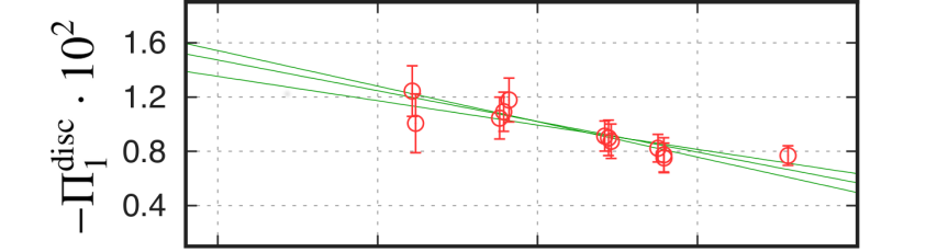
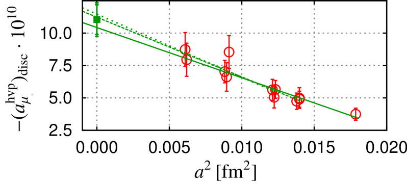
Figure 10: The continuum extrapolation of the quark-disconnected contribution to the leading time moment $\Pi_{1}$ of the vacuum polarisation function (top) and to $a_{\mu}^{\rm hvp}$ (bottom) computed by the BMW Collaboration [61, 65].

These results can be contrasted with a direct determination of the connected and disconnected contributions to the lowest two time moments, $\Pi_{1}$ and $\Pi_{2}$, calculated by the BMW Collaboration [61] at the physical pion mass. By employing a massive 6000 stochastic sources and exploiting stochastic noise cancellation between light and strange quark contributions [131], the disconnected contributions $\Pi_{1}^{\rm disc}$ and $\Pi_{2}^{\rm disc}$ could be well resolved. The upper panel of Figure 10 shows the continuum extrapolation of $\Pi_{1}^{\rm disc}$ computed at five different lattice spacings. One clearly sees that the leading disconnected contributions is negative. From the results of the two leading moments listed in Table II of Ref. [61] one can infer the Taylor expansion of the ratio $\Pi^{\rm disc}/\Pi^{\rm con}$ in the continuum limit as

$$\frac{\Pi^{\rm disc}}{\Pi^{\rm con}}(Q^{2})=-0.0166(25)+0.021(13)\left(Q^{2}\,[{\rm{GeV}}^{2}]\right)+{\rm{O}}(Q^{4}).$$ (96)

Hence, for $Q^{2}=0$, the ratio is given by $\Pi^{\rm disc}/\Pi^{\rm con}=-0.0166(25)$ which is $\approx-1/60$ and thus another factor two smaller in magnitude than the ChPT estimate of Ref. [82].

In two recent calculations the quark-disconnected contribution was computed at the physical value of the pion mass: The absolute magnitude of the disconnected part was found to be $(a_{\mu}^{\rm hvp})^{\rm{disc}}=-12.8(1.0)\cdot 10^{-10}$ by the BMW Collaboration [65] (see the lower panel of Figure 10 for a plot of the continuum extrapolation), while RBC/UKQCD [66] reported $(a_{\mu}^{\rm hvp})^{\rm{disc}}=-11.2(4.0)\cdot 10^{-10}$.

Collab.		$(a_{\mu}^{\rm hvp})_{\rm disc}\cdot 10^{10}$	$(a_{\mu}^{\rm hvp})_{\rm disc}/(a_{\mu}^{\rm hvp})_{\rm con}^{\ell\ell}$	$\Pi^{\rm disc}/\Pi^{\rm con}$	Comments
RBC/UKQCD		$-11.2(3.3)(2.3)$	$-1.6(6)\%$		$m_{\pi}=139\,{\rm{MeV}}$,
[58, 66]					domain wall fermions
BMW [61, 65]		$-12.8(1.0)(1.6)$	$-1.8(3)\%$	$-0.0166(25)$	$m_{\pi}=139\,{\rm{MeV}}$, cont. limit,
					staggered fermions
CLS/Mainz [62]			$>-2\%$		$m_{\pi}=437$ and $311\,{\rm{MeV}}$,
					Clover fermions
Bali & Endrődi				$-0.00036(45)$	$m_{\pi}=139\,{\rm{MeV}}$, $a=\,0.29\,{\rm{fm}}$,
[121]					staggered fermions
HSC 15 [144]		$-0.8(3)$	$-0.14(5)\%$		$m_{\pi}=391\,{\rm{MeV}}$, Clover fermions,
					smeared vector current

Table 3: Compilation of recent results for the quark-disconnected contribution to the hadronic vacuum polarisation. The result marked by an asterisk has been obtained from $(a_{\mu}^{\rm hvp})_{\rm disc}$ assuming $(a_{\mu}^{\rm hvp})_{\rm{con}}^{\ell\ell}=600\cdot 10^{-10}$.

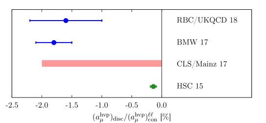
Figure 11: Ratio of the quark-disconnected and light quark-connected contribution to $a_{\mu}^{\rm hvp}$ as determined by RBC/UKQCD [66], BMW [65], CLS/Mainz [62] and HSC [144]. The red band denotes the range allowed by the lower bound determined via Eq. (93). The green circle indicates that the result has been obtained using smeared sources.

A compilation of recent results for the quark-disconnected contribution $(a_{\mu}^{\rm hvp})_{\rm disc}$, as well as the ratio $\Pi^{\rm disc}/\Pi^{\rm con}$ is shown in Table 3. With the recent determinations of Refs. [65] and [66] a consistent picture emerges: It is obvious that disconnected diagrams have only a minor influence on the total value of $a_{\mu}^{\rm hvp}$: their contribution is negative and amounts to $1.5-2$% in magnitude. This is also demonstrated by the plot shown in Figure 11.

In summary one finds that quark-disconnected contributions to $a_{\mu}^{\rm hvp}$ can nowadays be quantified reliably thanks to a number of technical improvements. Their overall magnitude is estimated to be at the level of a percent, which implies that they are important regarding the overall target precision. The accuracy achieved in the most recent determinations shows that they do not represent a serious obstacle for reaching the goal of making lattice calculations of $a_{\mu}^{\rm hvp}$ at least as precise as the dispersive analysis.

2.4 Finite-volume effects

As we shall see below, the effects induced by performing calculations in a finite volume lead to sizeable corrections when the minimum pion mass in units of the spatial box length satisfies $m_{\pi}L\approx 4$ . Obviously, a very accurate determination of finite-volume corrections is necessary, in order to estimate $a_{\mu}^{\rm hvp}$ with the desired level of overall precision.

The empirical evidence from calculations of hadron masses and decay constants suggests that finite-volume effects are negligibly small if the spatial box size $L$ satisfies $m_{\pi}L\gtrsim 4$, where $m_{\pi}$ is the actual value of the pion mass in the simulation. By contrast, the determination of $a_{\mu}^{\rm hvp}$ in lattice QCD appears to be much more sensitive to finite-size effects such that volumes in excess of $L=6\,{\rm{fm}}$ may be required.

Most estimates of finite-volume corrections that enter the current lattice QCD estimates of $a_{\mu}^{\rm hvp}$ are based on chiral effective field theory (EFT). There are also efforts to confront EFT estimates of finite-volume corrections with lattice data [145, 60], as well as scaling studies employing several different volumes [146]. There are some arguments that suggest that $m_{\pi}L\geq 6$ is necessary to suppress finite-volume sufficiently [62, 147], although more detailed studies are required to corroborate this.

One particular method to quantify finite-volume corrections is to consider anisotropy effects in the vacuum polarisation function $\Pi(Q^{2})$. The paper by Aubin et al. [145] starts from the observation that the vacuum polarisation tensor, $\Pi_{\mu\nu}(Q)$, does not vanish for $Q=0$ in a finite volume [94], contrary to what is expected from the tensor structure in Eq. (11), which is valid in infinite volume. It is then possible to construct the tensor $\overline{\Pi}_{\mu\nu}(Q)$ which has the zero mode subtracted and which satisfies the Ward-Takahashi identities. $\overline{\Pi}_{\mu\nu}(Q)$ contains five irreducible substructures that do not transform into each other under cubic rotations and which differ by finite-volume effects. In Ref. [145] the different irreducible substructures were computed in a lattice calculation employing rooted staggered quarks with $m_{\pi}=220\,{\rm{MeV}}$ and $m_{\pi}L=4.0$, as well as in chiral perturbation theory. While the effective chiral theory fails to reproduce the absolute value of the vacuum polarisation function, it describes the difference between different irreducible substructures quite well within the quoted statistical errors. The difference in the vacuum polarisation function due to finite volume effects can then be inserted into the convolution integral (see Eq. (13)), in order to determine the corresponding shift in $a_{\mu}^{\rm hvp}$. One finds that the correction amounts to $10-15$%. Thus, one concludes that the condition $m_{\pi}L=4$ at $m_{\pi}=220\,{\rm{MeV}}$ is not sufficient to guarantee that finite-volume effects are suppressed below the percent-level.

The observation that the assumption $\Pi_{\mu\nu}(0)=0$ does not hold in a finite volume has inspired the common practice of subtracting the zero mode via a simple modification of the phase factor in the Fourier transform of the vector correlator [94, 148], i.e.

$$\Pi_{\mu\nu}(Q)-\Pi_{\mu\nu}(0)=\int d^{4}x\,\left({\rm{e}}^{iQ\cdot x}-1\right)\left\langle J_{\mu}(x)J_{\nu}(0)\right\rangle\stackrel{{\scriptstyle!}}{{=}}(Q_{\mu}Q_{\nu}-\delta_{\mu\nu})\Pi(Q^{2}).$$ (97)

As discussed in [146], the subtraction of the zero mode leads to much smaller finite-volume effects in the determination of $\Pi(Q^{2})$ and, in turn, the estimate of $a_{\mu}^{\rm hvp}$.

Another approach to quantify finite-volume corrections and effects arising from the mass splitting between different “tastes” in the rooted staggered fermion formulation was presented in [60]. The starting point is an effective theory of photons, pions and $\rho$-mesons, similar to that used in [15]. This set-up can be used to compute the subtracted vacuum polarisation function in terms of an integral over the four-momentum. The coefficients in the Taylor expansion are related to the time moments. Their shift due to the finite volume can then be worked out by replacing the integral with a discrete sum over the Fourier modes and averaging over the multiplets related by the taste symmetry. The overall finite-volume correction to the estimate of $a_{\mu}^{\rm hvp}$ is estimated to be 7%.

We are now going to present a more detailed discussion of a dynamical theory of finite-volume effects, which uses as input the mass ratio $m_{\pi}/m_{\rho}$, as well as the box size in units of the pion mass, $m_{\pi}L$. This method is based on the time-momentum representation, and a detailed account can be found in [81, 62]. The goal is to compute the difference of the spatially summed vector correlator in infinite and finite volume, $G(x_{0},\infty)-G(x_{0},L)$. When inserted in Eq. (26), the finite-volume shift is determined. At short distances, i.e. for $x_{0}\lesssim 1\,{\rm{fm}}$ the Poisson resummation formula based on non-interacting pions should provide a good approximation for $G(x_{0},\infty)-G(x_{0},L)$. The long-distance contribution ($x_{0}\gtrsim 1\,{\rm{fm}}$) to the finite-size effect can be determined by invoking the Lüscher formalism using the low-lying energy eigenstates on a torus.

The integral representation for the short-distance part reads [81, 62]

$$G(x_{0},L)-G(x_{0},\infty)=\frac{1}{3}\left\{\frac{1}{L^{3}}\sum_{{\boldsymbol{n}}}-\frac{1}{(2\pi)^{3}}\int d^{3}k\right\}\frac{{\boldsymbol{k}^{2}}}{{\boldsymbol{k}^{2}+m_{\pi}^{2}}}{\rm{e}}^{-2x_{0}\sqrt{{{\boldsymbol{k}}}^{2}+m_{\pi}^{2}}}$$ (98)

$$\phantom{=}=\frac{m_{\pi}^{4}x_{0}}{3\pi^{2}}\sum_{\boldsymbol{n}\neq\boldsymbol{0}}\left\{\frac{K_{2}\left(m_{\pi}\sqrt{L^{2}{\boldsymbol{n}}^{2}+4x_{0}^{2}}\,\right)}{m_{\pi}^{2}(L^{2}{\boldsymbol{n}}^{2}+4x_{0}^{2})}\right.$$ (99)

$$\left.\phantom{\sum_{\boldsymbol{n}\neq\boldsymbol{0}}\frac{K_{2}\left(m_{\pi}\sqrt{L^{2}}\right)}{m_{\pi}^{2}(L^{2})}}-\frac{1}{m_{\pi}L|\boldsymbol{n}|}\int\limits_{1}^{\infty}dy\,K_{0}\left(m_{\pi}y\sqrt{L^{2}{\boldsymbol{n}}^{2}+4x_{0}^{2}}\,\right)\,\sinh\left(m_{\pi}L|\boldsymbol{n}|(y-1)\right)\right\},$$

where $K_{0},K_{2}$ denote modified Bessel functions of the second kind. Numerical estimates for the finite-volume shift in $a_{\mu}^{\rm hvp}$ have been worked out for the two-flavour CLS ensembles used in [56, 62]. It turns out that in the region where $x_{0}\lesssim 1\,{\rm{fm}}$ finite-volume corrections are negligibly small for $m_{\pi}L\geq 4$ and $m_{\pi}\lesssim 300\,{\rm{MeV}}$.

In order to determine finite-volume effects at large distances, i.e. in the case of interacting pions, we can rely on our earlier discussion in Section 2.2.3 on constraining the long-distance part of the iso-vector correlator. The iso-vector vector correlator in infinite volume is expressed in terms of the spectral function $\rho(\omega)$ as

$$G^{\rho\rho}(x_{0},\infty)=\int_{0}^{\infty}d\omega\,\omega^{2}\rho(\omega^{2})\,{\rm{e}}^{-\omega|x_{0}|},$$ (100)

with the $\pi\pi$ contribution given by

$$\rho(\omega^{2})=\frac{1}{48\pi^{2}}\left(1-\frac{4m_{\pi}^{2}}{\omega^{2}}\right)^{3/2}\left|F_{\pi}(\omega)\right|^{2}.$$ (101)

Above the threshold $\omega=2m_{\pi}$ the phase of the timelike pion form factor $F_{\pi}(\omega)$ is equal to the $p$-wave pion scattering phase shift $\delta_{11}(k)$, according to Watson’s theorem:

$$F_{\pi}(\omega)=\left|F_{\pi}(\omega)\right|{\rm{e}}^{i\delta_{11}(k)}.$$ (102)

In finite volume the correlator is given by Eq. (35), i.e. $G^{\rho\rho}(x_{0},L)=\sum_{n}|A_{n}|^{2}\,{\rm{e}}^{-\omega_{n}x_{0}}$. The discrete energy levels $\omega_{n}$ are related to the infinite-volume phase shifts by the Lüscher condition (see Eq. (36)), while the amplitudes $|A_{n}|^{2}$ are related to the timelike pion form factor according to Eq. (38). The determination of both $G^{\rho\rho}(x_{0},\infty)$ and $G^{\rho\rho}(x_{0},L)$ rely on input data for $F_{\pi}(\omega)$. The Gounaris-Sakurai parameterisation [149] of $F_{\pi}(\omega)$ proves helpful in this case. It describes the $\rho$-resonance in terms of two free parameters, $m_{\rho}$ and $\Gamma_{\rho}$. The expression for $F_{\pi}(\omega)$ reads

$$F_{\pi}(\omega)={f_{0}}\left/{\frac{k^{3}}{\omega}[\cot\delta_{11}(k)-i]}\right.,$$ (103)

and if one defines $k_{\rho}$ via $m_{\rho}=2\sqrt{k_{\rho}^{2}+m_{\pi}^{2}}$ one can express the phase shift $\delta_{11}(k)$ and the quantity $f_{0}$ in terms of $k_{\rho}$ and $\Gamma_{\rho}$.

In order to determine the iso-vector correlator $G^{\rho\rho}(x_{0},\infty)$ in infinite volume, one can use the values of $m_{\pi}$ and $m_{\rho}$ computed on a given ensemble and evaluate $k_{\rho}$ and $\Gamma_{\rho}$, assuming that $\Gamma_{\rho}\propto k_{\rho}^{3}/m_{\rho}^{2}$. Since $k$ is related to $\omega$ by $\omega=2\sqrt{k^{2}+m_{\pi}^{2}}$ in infinite volume, one can then evaluate $k^{3}\cot\delta_{11}(k)/\omega$ and $f_{0}$, and insert the result for $|F_{\pi}(\omega)|$ into Eq. (100).

In finite volume one uses $m_{\pi},m_{\rho}$ as before to determine $\delta_{11}(k)$ and $|F_{\pi}(\omega)|$. Both quantities then serve as input to solve the Lüscher condition, Eq. (36), as well as Eq. (38) for $n=1,2,\ldots.$ In this way one obtains both the finite-volume energy levels $\omega_{n}$ and the corresponding matrix elements $A_{n}$, which are used to evaluate $G^{\rho\rho}(x_{0},L)$ of Eq. (35). The resulting difference $G^{\rho\rho}(x_{0},\infty)-G^{\rho\rho}(x_{0},L)$ can then be used to determine the finite-volume shift $a_{\mu}^{\rm hvp}(\infty)-a_{\mu}^{\rm hvp}(L)$.

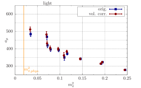
Figure 12: The ight quark contribution to the hadronic vacuum polarisation, $(a_{\mu}^{\rm hvp})^{ud}$, computed by CLS/Mainz [62] in two-flavour QCD. Filled red circles and blue squares denote the results with and without the finite-volume shift, respectively. The largest correction of $5.2\%$ is observed at the lightest pion mass of $\approx 190\,{\rm{MeV}}$.

This procedure has been applied by the Mainz group to determine the finite-volume shifts for $a_{\mu}^{\rm hvp}$ determined using the time-momentum representation [62]. Figure 12 shows the estimates for the hadronic vacuum polarisation contribution of the light quarks as a function of the pion mass, with and without the finite-volume shift. The largest correction of $(a_{\mu}^{\rm hvp}(\infty)-a_{\mu}^{\rm hvp}(L))/a_{\mu}^{\rm hvp}(\infty)=5.2\%$ is encountered for $m_{\pi}\approx 190\,{\rm{MeV}}$ at $m_{\pi}L=4.0$. In order to check the stability of the finite-volume shifts one can consider variations of the Gounaris-Sakurai parameters $m_{\rho},\Gamma_{\rho}$, as well as the Euclidean time at which one switches from considering non-interacting pions and the Poisson formula to the interacting case. In this way one can assign a 20% systematic uncertainty to the estimate of $a_{\mu}^{\rm hvp}(\infty)-a_{\mu}^{\rm hvp}(L)$. After applying the correction to each ensemble and performing a simultaneous chiral and continuum extrapolation one finds a finite-volume shift of 6.7% at the physical point.

Preliminary results by CLS/Mainz obtained in QCD with $2+1$ flavours of O($a$) improved Wilson fermions suggest that the above procedure is able to quantify the finite-volume correction quite accurately. By computing the correlator $G^{ud}(x_{0})$ on two different volumes, corresponding to $L=2.7$ fm and 4.1 fm, respectively one observes a significant finite-volume shift for the integrand $w(x_{0})\,G^{ud}(x_{0})$. Applying the finite-volume correction determined via the timelike pion form factor and the Lüscher procedure makes the results obtained on the two volumes compatible within statistical errors.

Another direct comparison of results for $a_{\mu}^{\rm hvp}$ obtained on two different volumes has been reported by the PACS collaboration [147]. Employing $2+1$ flavours of O($a$) Wilson quarks on lattice sizes of $96^{4}$ and $64^{4}$ at $a=0.085$ fm, which correspond to box lengths of $L=8.1$ fm and 5.4 fm, respectively, they study the volume dependence of the integrand $w(x_{0})\,G(x_{0})$ of the time-momentum representation, as well as the estimate for $a_{\mu}^{\rm hvp}$ resulting from the integration up to $x_{0}^{\rm{cut}}\approx 3$ fm. At their reference pion mass of 146 MeV they find an absolute finite-volume correction of

$$a_{\mu}^{\rm hvp}(L=8.1\,{\rm{fm}})-a_{\mu}^{\rm hvp}(L=5.4\,{\rm{fm}})=(10\pm 26)\cdot 10^{-10}$$ (104)

for the light quark contribution to $a_{\mu}^{\rm hvp}$. The central value of this estimate agrees well with the result obtained using chiral EFT [145]. One concludes that, at near-physical pion mass, the finite-volume correction between ensembles with $m_{\pi}L\approx 4$ and $m_{\pi}L\approx 6$ amounts to 1.5%, although the shift is not statistically significant.

2.5 Chiral extrapolation of $a_{\mu}^{\rm hvp}$

Simulations of lattice QCD at parameter values that correspond to the physical pion mass have become routine. However, in some cases the result at the physical point is still obtained by chirally extrapolating the data obtained for pion masses in the range of $200-400\,{\rm{MeV}}$. Furthermore, results computed directly at the physical value of $m_{\pi}$ are often combined with data at larger masses in order to increase the overall accuracy, and in many cases the final estimate is obtained through a simultaneous chiral and continuum extrapolation. Results from the first comprehensive calculations of $a_{\mu}^{\rm hvp}$ on the lattice [54, 55, 56] showed a strong dependence of $a_{\mu}^{\rm hvp}$ on $m_{\pi}^{2}$. In Ref. [54] it was observed that this behaviour was correlated with a strong variation of the $\rho$-meson mass with $m_{\pi}$. Hence, in order to produce a milder dependence of $a_{\mu}^{\rm hvp}$ on the pion mass, the authors of Ref. [54] proposed a rescaling of the momentum $Q^{2}$ of the subtracted vacuum polarisation according to

$$\hat{\Pi}(Q^{2})\to\hat{\Pi}(hQ^{2}),\quad h=\frac{m_{\rm V}^{2}}{m_{\rho}^{2}},$$ (105)

where $m_{\rho}$ is the physical $\rho$-meson mass, while $m_{\rm V}$ denotes its value computed for the actual pion mass of a given gauge ensemble. The fact that the rescaling factor $h$ approaches unity as $m_{\pi}$ is tuned towards its physical value implies that the limits of $a_{\mu}^{\rm hvp}$ computed with or without rescaling are the same.

The motivation for the rescaling can be derived from a simple consideration based on vector meson dominance [56, 150]. In the VMD model the $Q^{2}$-dependence of the hadronic vacuum polarisation in the iso-vector channel is given by

$$\hat{\Pi}(Q^{2})_{\rm VMD}(Q^{2})\sim g_{\rm V}\frac{Q^{2}}{Q^{2}+m_{\rm V}^{2}},$$ (106)

where $g_{\rm V}$ is related to the $\rho$-meson decay constant. Assuming that $m_{\rm V}$ depends strongly on $m_{\pi}$ while $g_{\rm V}$ does not, one easily sees that the rescaling of $Q^{2}$ according to Eq. (105) makes $\hat{\Pi}(Q^{2})_{\rm VMD}$ broadly independent of the pion mass, and the same will be true for the resulting value of $a_{\mu}^{\rm hvp}$ after evaluating the convolution integral of Eq. (13). In [60], a variant of the method was considered, which combines the rescaling with the subtraction of the relative pion loop correction computed in chiral effective theory at NLO between the physical and actual values of $m_{\pi}$. Indeed, one finds that the chiral behaviour of $a_{\mu}^{\rm hvp}$ is much flatter as a result of multiplying $Q^{2}$ by ${m_{\rm{V}}^{2}}/{m_{\rho}^{2}}$ [54, 60].

The stability of the chiral extrapolation of $a_{\mu}^{\rm hvp}$ was analysed extensively in Ref. [150] using a model for the iso-vector vacuum polarisation derived from ChPT at two loops and the experimentally determined spectral function. By comparing several ansätze for the chiral extrapolation of the hadronic vacuum polarisation determined for pion masses in the range $200-400\,{\rm{MeV}}$ it was found that the typical spread of $a_{\mu}^{\rm hvp}$ at the physical pion mass is of the order of 5%. Importantly, while the rescaling helps to produce a flatter pion mass dependence, there remains an ambiguity arising from different model functions for the chiral fit, none of which is clearly preferred on theoretical grounds. The authors of Ref. [150] conclude that extrapolations from pion masses larger than 200 MeV are not reliable enough to achieve sub-percent level precision.

2.6 Scale setting

A source of systematic uncertainty that received little attention in early calculations of $a_{\mu}^{\rm hvp}$ is the error on the lattice scale [62, 117]. Although $a_{\mu}^{\rm hvp}$ is a dimensionless quantity, there are two ways in which the lattice scale enters the calculation. This is most easily explained in the framework of the time-momentum representation of $a_{\mu}^{\rm hvp}$ defined in Eq. (26): Firstly, the muon mass $m_{\mu}$ enters the kernel function $w(x_{0})$ via the dimensionless combination $x_{0}m_{\mu}$. Secondly, the masses of the dynamical quarks enter implicitly via the lattice evaluation of the vector correlator. Therefore, $a_{\mu}^{\rm hvp}$ can be thought of as a function in the dimensionless variables $M_{\mu}\equiv m_{\mu}/\Lambda,M_{u}\equiv m_{u}/\Lambda,M_{d}\equiv m_{d}/\Lambda,\ldots$, where $\Lambda$ is the quantity that sets the lattice scale. The scale setting error $\Delta\Lambda$ then induces a corresponding uncertainty in $a_{\mu}^{\rm hvp}$, i.e.

$$\Delta a_{\mu}^{\rm hvp}=\bigg{|}\Lambda\frac{da_{\mu}^{\rm hvp}}{d\Lambda}\bigg{|}\,\frac{\Delta\Lambda}{\Lambda}=\bigg{|}M_{\mu}\frac{\partial a_{\mu}^{\rm hvp}}{\partial M_{\mu}}+\sum_{f=1}^{N_{\rm f}}M_{\rm f}\frac{\partial a_{\mu}^{\rm hvp}}{\partial M_{\rm f}}\bigg{|}\,\frac{\Delta\Lambda}{\Lambda}.$$ (107)

Often one employs a hadronic renormalisation scheme in which the quark masses are expressed in terms of suitable meson masses. For instance, in the isospin limit one can fix the average light quark mass $m_{ud}\equiv\frac{1}{2}(m_{u}+m_{d})$ by the pion mass $m_{\pi}$, which can be easily generalised to apply to heavier quark flavours, too. The uncertainty $\Delta a_{\mu}^{\rm hvp}$ can then be written as

$${\Delta a_{\mu}^{\rm hvp}}=\bigg{|}M_{\mu}\frac{\partial a_{\mu}^{\rm hvp}}{\partial M_{\mu}}+M_{\pi}\frac{\partial a_{\mu}^{\rm hvp}}{\partial M_{\pi}}+M_{\rm K}\frac{\partial a_{\mu}^{\rm hvp}}{\partial M_{\rm K}}+\ldots\bigg{|}\,\frac{\Delta\Lambda}{\Lambda},$$ (108)

where $M_{\pi},M_{\rm K},\ldots$ denote the meson masses in units of $\Lambda$. In the time-momentum representation one can determine the derivative term involving the muon mass via [62]

$$M_{\mu}\frac{\partial a_{\mu}^{\rm hvp}}{\partial M_{\mu}}=-a_{\mu}^{\rm hvp}+\left(\frac{\alpha}{\pi}\right)^{2}\int_{0}^{\infty}dx_{0}\,G(x_{0})\,J(x_{0}),\quad J(x_{0})=x_{0}w^{\prime}(x_{0})-w(x_{0}),$$ (109)

where $w^{\prime}(x_{0})$ denotes the derivative of the kernel function $w(x_{0})$ in Eq. (27). Both $w(x_{0})$ and $w^{\prime}(x_{0})$ can be easily computed using the series expansion from appendix B in [62]. Moreover, in the same paper the derivative with respect to the pion mass $M_{\pi}$ has been determined from the slope of the chiral extrapolation at $m_{\pi}=m_{\pi}^{\rm{phys}}$. In this way one finds

$$\frac{\Delta a_{\mu}^{\rm hvp}}{a_{\mu}^{\rm hvp}}=\Bigg{|}\underbrace{\frac{M_{\mu}}{a_{\mu}^{\rm hvp}}\frac{\partial a_{\mu}^{\rm hvp}}{\partial M_{\mu}}}_{\displaystyle{1.8}}+\underbrace{\frac{M_{\pi}}{a_{\mu}^{\rm hvp}}\frac{\partial a_{\mu}^{\rm hvp}}{\partial M_{\pi}}}_{\displaystyle{-0.18(6)}}\Bigg{|}\,\frac{\Delta\Lambda}{\Lambda}.$$ (110)

Thus, the factor multiplying the scale setting uncertainty is dominated by the contribution from the muon mass, with only a 10% reduction coming from the light quarks. Heavier quark flavours are likely to have an even smaller effect. One concludes from this analysis that the proportionality between the relative uncertainties of $a_{\mu}^{\rm hvp}$ and the lattice scale $\Lambda$ is a number of order one. Therefore, the lattice scale must be known to within a fraction of a percent, if one is to reach the precision goal in the determination of $a_{\mu}^{\rm hvp}$.

2.7 Isospin-breaking effects

Controlling and quantifying the effects from isospin breaking is of major importance for the determination of $a_{\mu}^{\rm hvp}$. In the phenomenological approach based on the hadronic cross section ratio $R(s)$, it is necessary to include the contributions from final state radiation [4], $\pi^{0}\gamma$ and $\eta\gamma$ channels [14], as well as $\rho\omega$ mixing [151, 15]. The latter, in particular, played a vital rôle in arriving at a consistent estimate of the iso-vector $\pi\pi$-contribution to $a_{\mu}^{\rm hvp}$ using data from either $e^{+}e^{-}\to\pi^{+}\pi^{-}$ or, alternatively, from hadronic $\tau$-decays [15]. In total, isospin breaking effects account for 1.3% of the dispersive estimate for $a_{\mu}^{\rm hvp}$ and represent a crucial ingredient for reaching the current level of precision.

The treatment of isospin breaking in lattice QCD has been a major focus of recent activity. The inclusion of isospin breaking effects in lattice calculations of $a_{\mu}^{\rm hvp}$ is indispensable for the goal of reaching sub-percent precision. There are two sources of isospin breaking: (1) the strong interaction contribution that arises from the mass splitting between the up and down quarks, $m_{u}\neq m_{d}$, which is of order $\alpha^{2}(m_{d}-m_{u})$, and (2) electromagnetic corrections of O($\alpha^{3}$) due to the different electric charges of the quarks.

The inclusion of electromagnetism in a manner that is consistent with the lattice formulation of QCD is technically challenging. As discussed in a recent review article [79], Gauss’s law forbids the existence of states with non-zero electric charge in a finite volume with periodic boundary conditions. Another way of expressing this obstacle is the statement that charged states do not propagate in a finite periodic box: Large gauge transformations that are admitted by the boundary conditions cannot be eliminated by any local gauge-fixing procedure.

Since the photon is a massless unconfined particle, the finite-volume effects of lattice QCD in the presence of electromagnetism must be reassessed. In particular, one expects finite-volume effects to be more severe, since the leading corrections fall off as powers of the inverse volume instead of exponentially [152]. In order to circumvent these problems several prescriptions have been pursued. The starting point is the Euclidean path integral of QCD and QED

$$Z_{\rm QCD+QED}=\int D[U]D[A]D[\overline{\psi},\psi]\,{\rm e}^{-S_{\gamma}[A]-S_{\rm G}[U]-S_{\rm F}[U,A,\overline{\psi},\psi]},$$ (111)

where $S_{\gamma}[A]$ denotes the photon action, and $A_{\mu}(x)$ represents the photon field. Usually one employs the non-compact formulation of QED in which the action – including a gauge-fixing term – is given by

$$S_{\gamma}[A]=a^{4}\sum_{x}\left\{\frac{1}{4}\sum_{\mu,\nu}\left(\nabla_{\mu}A_{\nu}-\nabla_{\nu}A_{\mu}\right)^{2}+\frac{1}{2\xi}\left(\sum_{\mu}\nabla_{\mu}A_{\mu}(x)\right)^{2}\right\},$$ (112)

where $\nabla_{\mu}$ denotes the forward lattice derivative. Below we outline several prescriptions that have been pursued to circumvent the conceptual problems of QED in a finite volume.

• In the QED_TL prescription, originally proposed in Ref. [152], the zero modes of the photon field are explicitly set to zero by imposing

  $$\left.\widetilde{A}_{\mu}(p)\right|_{p=0}\equiv\int d^{4}x\,A_{\mu}(x)=0,$$ (113)

  where $\widetilde{A}_{\mu}(p)$ denotes the photon field in Fourier space. As this is a non-local constraint, the path integral in Eq. (111) does not admit a representation in terms of the transfer matrix, and hence the Hamiltonian cannot be defined.

• The QED_L prescription [153] imposes a different constraint, i.e.

  $$\int d^{3}x\,A_{\mu}(x_{0},\boldsymbol{x})=0,$$ (114)

  which corresponds to setting all spatial zero modes of the photon field to zero. Since this condition is local in time, the theory does admit a Hamiltonian. However, the non-locality in space spoils the renormalisation of local composite operators with dimensions larger than four [79].

• In the formulation of Ref. [154], proposed originally to study the infrared properties of QED, one imposes a cutoff on the value of the zero mode. The existence of a transfer matrix is not guaranteed.

• Alternative treatments include the QED_m prescription which introduces a massive photon [155], and the formulation based on the introduction of C-parity boundary conditions, called QED_C [156, 157]. While both are consistent quantum field theories, one finds that QED_m requires a careful treatment of the limits $m_{\gamma}\to 0$ and $L\to\infty$. The QED_C formulation breaks flavour symmetry, but as the breaking is local, the effects of flavour symmetry breaking are exponentially suppressed.

Two distinct approaches are widely applied in calculations of observables in the presence of strong and electromagnetic isospin breaking. The first is the “stochastic method”: It is based on the direct Monte Carlo evaluation of the path integral in Eq. (111). The coupling of the photon $A_{\mu}(x)$ to the quark fields is accomplished by augmenting the link variables describing the gluons by a U(1) phase factor according to

$$U_{\mu}(x)\to{\rm{e}}^{ieA_{\mu}(x)}U_{\mu}(x),$$ (115)

where $e$ is the electric charge. In order to facilitate the stochastic calculation of observables defined with respect to $Z_{\rm QCD+QED}$ the sea quarks are assumed to be electrically neutral, so that the U(1) gauge field is generated independently from the SU(3) gauge fields. This defines the so-called “electro-quenched” approximation which has been applied very successfully to determine electromagnetic mass splittings among hadrons, as well as the up-down quark mass difference (see Refs. [152, 158, 68, 76, 77, 159, 160, 161, 162]). Strong isospin breaking is either incorporated by choosing different up and down quark masses, as was done, for instance, in [77] or via reweighting techniques (an example is discussed in Ref. [163]).

The second method for determining isospin breaking effects arising from electromagnetic corrections is based on the perturbative expansion of the path integral of Eq. (111) in powers of the fine structure constant $\alpha$ [72]. In a similar manner, strong isospin breaking effects can be treated in this framework by expanding the path integral in powers of the light quark mass difference $(m_{d}-m_{u})$ [71].

We will now discuss several recent lattice calculations of isospin-breaking effects in $a_{\mu}^{\rm hvp}$. The RBC/UKQCD Collaboration has studied electromagnetic corrections using the QED_L prescription at a pion mass of 340 MeV and focussing on connected diagrams only [70]. By performing a detailed comparison of the stochastic and perturbative methods they conclude that, while both yield consistent results of similar accuracy, the stochastic approach fares slightly better in terms of numerical accuracy. In a follow-up paper [66] they present a calculation of both strong and electromagnetic isospin-breaking contributions based on the perturbative method and at the physical pion mass. The finite-volume corrections of order $1/L$ and $1/L^{2}$ are removed, a subset of QED-disconnected graphs is included, and strong isospin-breaking effects have been included by computing the leading-order graphs arising in the expansion in $(m_{u}-m_{d})$. The isospin-breaking corrections to the renormalisation factor of the electromagnetic current have also been included. In this way they obtain a total isospin-breaking correction to $a_{\mu}^{\rm hvp}$ of $(9.5\pm 10.4)\cdot 10^{-10}$, which amounts to $+(1.5\pm 1.6)$% of the iso-symmetric contribution from up and down quarks. It is interesting to note that the contribution from strong isospin breaking alone is $(10.6\pm 8.0)\cdot 10^{-10}$, indicating that the dominant effect is due to $m_{u}\neq m_{d}$.

The ETM Collaboration [63] has used the QED_L prescription together with the perturbative approach to determine the electromagnetic corrections to the strange and charm quark contributions, $(a_{\mu}^{\rm hvp})^{s}$ and $(a_{\mu}^{\rm hvp})^{c}$. Neglecting disconnected diagrams and extrapolating results to the physical pion mass and vanishing lattice spacing, they find that electromagnetic corrections to $(a_{\mu}^{\rm hvp})^{s}$ and $(a_{\mu}^{\rm hvp})^{c}$ amount to $-0.03$ % and $-0.21$ %, respectively, which is negligible relative to the statistical error of the iso-symmetric contribution.

The calculation by the Fermilab-HPQCD-MILC Collaboration [64] is focussed on the determination of the strong isospin-breaking correction alone. Using two ensembles at the physical pion mass – one in the iso-symmetric limit, i.e. with $m_{u}=m_{d}$, and another one that realises a splitting between up and down quark masses consistent with an earlier calculation [64] – they are able to test strong isospin-breaking effects arising from the quark sea as well. Their main result for the strong isospin correction in $a_{\mu}^{\rm hvp}$ is $(9.0\pm 2.3\pm 3.1)\cdot 10^{-10}$, where the second error is the total systematic error which is dominated by the neglected quark-disconnected contribution. Combining this result with the iso-symmetric light quark contribution to $a_{\mu}^{\rm hvp}$ of Ref. [60], the relative shift is $+(1.5\pm 0.7)$%.

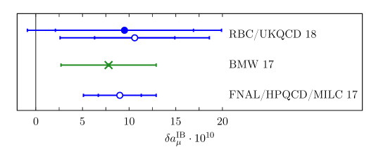
Figure 13: Compilation of determinations of the isospin-breaking correction $\delta a_{\mu}^{\rm IB}$ to the hadronic vacuum polarisation, computed by RBC/UKQCD [66], BMW [65] and Fermilab/HPQCD/MILC [64]. Circles denote results computed in lattice QCD, while the green cross represents the phenomenological estimate used in the calculation by BMW. Strong isospin-breaking contributions are shown as open circles.

The estimate of isospin-breaking effects in the result of the BMW Collaboration [65] has not been determined by a lattice calculation but instead by phenomenology. The contributions from the $\pi^{0}\gamma$ and $\eta\gamma$ channel have been taken over from the dispersive approach, final-state radiation has been estimated using a combination of data and point-particle QED corrections, and hadronic models have been used to estimate the contribution from $\rho$-$\omega$ mixing. The slight detuning of the pion mass has been corrected for using leading-order chiral EFT. The total correction due to isospin breaking is found to be $(7.8\pm 5.1)\cdot 10^{-10}$ or $+(1.2\pm 0.8)$ % of the light-quark iso-symmetric contribution.

Thanks to the considerable effort invested, a coherent picture emerges regarding the isospin-breaking contribution $\delta a_{\mu}^{\rm IB}$ to $a_{\mu}^{\rm hvp}$: as is evident from the compilation in Figure 13, the correction is positive and of order $10\cdot 10^{-10}$, which amounts to about 1.5% of the total leading-order hadronic vacuum polarisation. In view of the target precision, this is a significant correction. Moreover, the calculations of RBC/UKQCD [66] and FNAL/HPQCD/MILC [64] show that the size of $\delta a_{\mu}^{\rm IB}$ is dominated by strong isospin-breaking effects. The fact that electromagnetic corrections are small and negligible relative to the statistical errors in current calculations has also been confirmed by ETMC [63]. It is also interesting to note that isospin-breaking corrections to $a_{\mu}^{\rm hvp}$ are similar in size compared to the quark-disconnected contribution, but come in with the opposite sign.

Clearly, the precision of these calculations must be further increased, since the errors quoted for $\delta a_{\mu}^{\rm IB}$ amount to $50-100$ %. It is also important to note that the mass difference between the charged and neutral pions must be treated in a consistent manner, in order to guarantee a reliable determination of isospin-breaking effects.

2.8 Results for $a_{\mu}^{\rm hvp}$

We will now discuss the available results from lattice QCD calculations of $a_{\mu}^{\rm hvp}$, assess their level of accuracy and compare them to estimates based on dispersion relations. We begin by presenting short accounts of the individual calculations whose results are listed in Table 4, with additional information on simulation details given in Table 5.

Aubin and Blum [53] performed the first determination of $a_{\mu}^{\rm hvp}$ using $N_{\rm f}=2+1$ flavours of staggered quarks, following the strategy outlined in [51]. By fitting the $Q^{2}$-dependence of $\Pi(Q^{2})$ to the functional form predicted by staggered ChPT, they determined $a_{\mu}^{\rm hvp}$ at a single value of the lattice spacing and three pion masses in the range $240-470\,{\rm{MeV}}$. The results were extrapolated to the physical pion mass using either a linear or quadratic ansatz in $m_{\pi}^{2}$. Contributions from the charm quark were not included, and the quoted errors are purely statistical.

The calculations by the ETM Collaboration [54, 57] were performed using twisted mass QCD as the discretisation of the quark action. One of the main features of their analysis is the rescaling of the squared momentum $Q^{2}$ in the argument of $\Pi(Q^{2})$ according to Eq. (105). In Ref. [54] it was argued (see also [56]) that this rescaling results in a much milder pion mass dependence, leading to a more stable chiral extrapolation to the physical point. The first calculation [54] was performed in two-flavour QCD, considering only the $u,d$ contributions to the hadronic vacuum polarisation. No significant dependence on the lattice spacing, the volume and the details of the chiral extrapolation were observed at the level of statistical precision. Quark-disconnected contributions were computed but found to be zero within errors. The second calculation was performed for tmQCD with $N_{\rm f}=2+1+1$ dynamical flavours at three different lattice spacings. Systematic uncertainties were estimated from variations in the fit ansatz used to describe the low-$Q^{2}$ regime and by considering different fit intervals in the determination of the vector meson mass $m_{\rm V}$ which enters the rescaling factor in Eq. (105). No appreciable change in the result was observed when ensembles with $m_{\pi}L<4$ were excluded from the analysis, and hence they concluded that volume effects were small. In their 2017 paper [63], ETM presented results for the strange and charm quark contributions (which had not been quoted as separate quantities in [57]), including the corrections from electromagnetism. As was already discussed in Section 2.7, the latter were found to be much smaller than the overall statistical uncertainty.

CLS/Mainz [56, 62] have determined $a_{\mu}^{\rm hvp}$ using two flavours of ${\rm{O}}(a)$ improved Wilson fermions at three lattice spacings and pion masses from $190-500\,{\rm{MeV}}$. Twisted boundary conditions were employed to realise smaller values of $Q^{2}$ and a high density of points to describe the $Q^{2}$-dependence of the vacuum polarisation function. The overall precision of the earlier result [56] amounts to 10% with the main systematic uncertainty arising from the uncertainty in the lattice scale. The more recent publication [62] contains a detailed comparison of the different methods to determine $a_{\mu}^{\rm hvp}$, i.e. the hybrid method, the time-momentum representation and time moments. Finite-volume corrections were determined using the Gounaris-Sakurai model for the timelike pion form factor. The uncertainty in the final result is dominated by statistics, while the systematic error estimate includes the uncertainties due to variations in the analysis procedure, finite-volume corrections, scale setting and quark-disconnected diagrams. The calculations have now been extended to QCD with $N_{\rm f}=2+1$ flavours of dynamical quarks [117], including ensembles at the physical value of the pion mass. Special attention is given to constraining the long-distance regime of the spatially summed vector correlator via a dedicated calculation of the energies $\omega_{n}$ and associated amplitudes $A_{n}$ for the first four lowest-lying states in the iso-vector channel (see Eq. (35)), which also allows for the determination of the finite-volume shift via the timelike pion form factor.

The RBC/UKQCD Collaboration [55, 59, 66] employs domain wall fermions for the discretisation of the quark action. In their initial study [55] they studied eight different ensembles at three different lattice spacings to obtain a result for $a_{\mu}^{\rm hvp}$, yet without contributions from the charm quark and disconnected diagrams. By comparing the results from a chiral extrapolation with and without the rescaling factor of Eq. (105) no statistically significant difference between the two procedures was detected at the physical pion mass. Results were found to be stable against variations in the lattice spacing and volume in the accessible range. The calculation of the strange quark contribution $(a_{\mu}^{\rm hvp})^{s}$ reported in [59] was based on ensembles at the physical pion mass and two lattice spacings. The $Q^{2}$-dependence was studied extensively by employing the hybrid method of Ref. [85]. Systematic errors were estimated by considering a large number of procedural variations. In their latest paper [66] RBC/UKQCD presented a determination of $a_{\mu}^{\rm hvp}$ at two values of the lattice spacing and at the physical pion mass. Employing the time-momentum representation, the long-distance regime was constrained by the “bounding method” used also by the BMW Collaboration (see Figure 7). The total precision of the final result, which includes finite-volume corrections, quark-disconnected diagrams and isospin-breaking (QCD+QED) effects, is 2.6%. They also quote a far more precise estimate which is obtained through a combination of their lattice calculation of the correlator $G(x_{0})$ and experimentally determined cross section ratio $R(s)$. This is discussed further below.

Collaboration	$a_{\mu}^{\rm hvp}$	$(a_{\mu}^{\rm hvp})^{uds}$	$(a_{\mu}^{\rm hvp})^{ud}$	$(a_{\mu}^{\rm hvp})^{s}$	$(a_{\mu}^{\rm hvp})^{c}$	Method
$N_{\rm f}=2+1+1:$
BMW 17 [65]	711.0(7.5)(17.3)∗†	696.3(7.5)(17.3)∗†		53.7(0)(4)	14.7(0)(1)	TMR
ETMC 17 [63]				53.1(2.5)†	14.72(56)†	TMR
HPQCD 16 [60]	667(6)(12)∗†		599(11)∗†			Moments
HPQCD 14 [93]				53.4(6)	14.4(4)	Moments
ETMC 13 [57, 164]	674(21)(18)	655(21)		53(3)	14.1(6)	Fits in $Q^{2}$
$N_{\rm f}=2+1:$
	715.4(16.3)(9.2)∗†	701.2(16.3)(9.2)∗†		53.2(4)(3)	14.3(0)(7)	TMR
RBC/UKQCD 18 [66]	692.5(1.4)(0.5)(0.7)(2.1)∗†					$R$-ratio, TMR
RBC/UKQCD 16 [59]				53.1(9)(${}^{1}_{3}$)		Hybrid
RBC/UKQCD 11 [55]		641(33)(32)				Fits in $Q^{2}$
Aubin & Blum 07 [53]		713(15) / 748(25)				Fits in $Q^{2}$
$N_{\rm f}=2:$
CLS/Mainz 17 [62]	654(32)(${}^{21}_{23}$)∗	639(32)(${}^{21}_{23}$)∗	588(32)(${}^{21}_{23}$)	51.1(1.7)(0.4)	14.3(2)(1)	TMR
CLS/Mainz 11 [56]		618(64)				Fits in $Q^{2}$
ETMC 11 [54]			572(16)∗			Fits in $Q^{2}$

Table 4: Compilation of recent results for the hadronic vacuum polarisation contribution in units of $10^{-10}$. The method used to determine $a_{\mu}^{\rm hvp}$ is specified in the last column. Whenever contributions from quark-disconnected diagrams enter the estimate or the quoted error this is marked by an asterisk. Entries marked by a dagger have either been corrected for isospin-breaking effects or the corresponding uncertainty has been included in the error. Additional information on simulation details are given in Table 5.

Collaboration	Action	$a$ [fm]	$m_{\pi}^{\rm min}$ [MeV]	$m_{\pi}^{\rm min}L$	FV corr.
$N_{\rm f}=2+1+1:$
BMW 17 [65]	Staggered	$0.064,0.095,0.111,0.118,0.134$	139	4.3	ChEFT
ETMC 17 [63]	tmQCD	$0.062,0.082,0.089$	223	3.4	X
HPQCD 16 [60]	HISQ	$0.09,0.12,0.15$	133	3.9	ChEFT
HPQCD 14 [93]	HISQ	$0.09,0.12,0.15$	133	3.9	ChEFT
ETMC 13 [57, 164]	tmQCD	$0.062,0.078,0.086$	227	3.3	X
$N_{\rm f}=2+1:$
RBC/UKQCD 18 [66]	DWF	$0.084,0.114$	139	3.8	ChEFT
RBC/UKQCD 16 [59]	DWF	$0.084,0.114$	139	3.8	X
RBC/UKQCD 11 [55]	DWF	$0.084,0.114,0.143$	180	4.0	X
Aubin & Blum 07 [53]	Staggered	$0.086$	241	4.2	X
$N_{\rm f}=2:$
CLS/Mainz 17 [62]	Clover	$0.049,0.066,0.076$	185	4.0	GS
CLS/Mainz 11 [56]	Clover	$0.05,0.06,0.08$	277	4.0	X
ETMC 11 [54]	tmQCD	$0.063,0.079$	290	3.7	X

Table 5: Simulation details for the calculations of the hadronic vacuum polarisation contribution $a_{\mu}^{\rm hvp}$ listed in Table 4. The discretisation of the quark action is indicated in the second column (HISQ: highly improved staggered quarks; tmQCD: twisted mass QCD; DWF: domain wall fermions; Clover: O$(a)$ improved Wilson quarks). The column labelled “FV corr.”, indicate whether finite-volume corrections have been included, either via chiral effective field theory (ChEFT) or the formalism based on the Gounaris-Sakurai (GS) parameterisation.

The HPQCD Collaboration [93, 60] use ensembles with $N_{\rm f}=2+1+1$ flavours of “highly improved staggered quarks” (HISQ) to determine $a_{\mu}^{\rm hvp}$ by computing time moments. The large-$x_{0}$ regime of the vector correlator $G(x_{0})$ was constrained by performing multi-exponential fits using Bayesian priors. Ensembles at three different lattice spacings including physical pion masses enable a simultaneous chiral and continuum extrapolation of the moments from which the vacuum polarisation function $\Pi(Q^{2})$ was determined. The light quark contribution was corrected for finite-volume effects as well as taste-symmetry violations that manifest themselves as mass splittings among pions within a taste multiplet. Contributions from quark-disconnected diagrams were included in the final result and error. The effects of strong isospin-breaking were reported in a companion paper together with the Fermilab-HPQCD-MILC Collaboration [64]. The findings were already discussed in Section 2.7 of this review. The overall precision of the result quoted in [60] is 2.0%.

The BMW Collaboration [61, 65] has performed a comprehensive study using $N_{\rm f}=2+1+1$ flavours of staggered quarks at six values of the lattice spacing including physical pion masses and volumes that satisfy $m_{\pi}L\approx 4.3$. Thanks to the massive accumulated statistics (i.e. more than $10^{6}$ individual measurements for the contributions from up and down quarks and about $10^{5}$ measurements for strange and charm), they obtained very precise results and were also able to compute quark-disconnected diagrams for all four flavours. The infrared regime of the correlator was constrained via the “bounding method” (see Eq. (41)). The first paper [61] was focussed on the leading two time moments, $\Pi_{1}$ and $\Pi_{2}$, which can be used to constrain $a_{\mu}^{\rm hvp}$ via the Mellin moments discussed in Section 2.2.6 and the QCD sum rule approach of Section 2.2.7. The more recent publication [65] contains the result for $a_{\mu}^{\rm hvp}$ extrapolated to the continuum limit, including finite-volume corrections, quark-disconnected diagrams and a correction for isospin-breaking effects estimated from phenomenology (see Section 2.7). The overall precision is 2.7%.

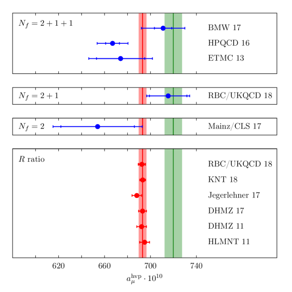
Figure 14: Compilation of recent results for the hadronic vacuum polarisation contribution in units of $10^{-10}$. The three panels represent calculations with different numbers of sea quarks. References for individual lattice calculations are listed in Table 4. The red vertical band denotes the estimate from dispersion theory quoted in DHMZ 17 [10], while the green band represents the “no new physics” scenario (see text). The other phenomenological determinations based on the $R$-ratio are labelled as HLMNT 11 [16], DHMZ 11 [14], Jegerlehner 17 [17] and KNT 18 [18].

In Figure 14 we show a compilation of recent results for the total leading-order hadronic vacuum polarisation contribution, while Figures 15 and 16 show recent estimates of the individual contributions from the strange and charm quarks to $a_{\mu}^{\rm hvp}$. The overall precision of current lattice calculations of $a_{\mu}^{\rm hvp}$ is at the level of 2.5%. Estimates are mostly dominated by systematics, with the largest uncertainties associated with finite-volume effects, the continuum extrapolation, isospin-breaking and scale setting. Constraining the infrared regime of the vector correlator also makes a sizeable contribution to the total error budget of the calculations shown and listed in Figure 14 and Table 4.

It is interesting to note that the results of ETMC 13 [57], HPQCD 16 [60] and CLS/Mainz 17 [62] are 3–5% lower than the phenomenological estimate, while the most recent estimates by BMW 17 [65] and RBC/UKQCD 18 [66] are larger by 3%. By contrast, lattice estimates for the individual strange and charm quark contributions are quite compatible among different collaborations, as indicated in Figures 15 and 16. This confirms that the contribution from the light quark flavours not only accounts for the bulk of the HVP contribution but is also mainly responsible for the accuracy of current lattice calculations. In Figure 14 the lattice results for $a_{\mu}^{\rm hvp}$ are also compared to the estimates obtained by evaluating the dispersion integral using the experimentally measured cross section ratio for $e^{+}e^{-}\to\rm hadrons$ in the low-energy regime. Clearly, the uncertainties of the phenomenological approach are much smaller, implying that the overall precision of lattice calculations must be improved by a factor $\sim 5$.

Figure 14 also shows that the estimates from BMW 17 and RBC/UKQCD 18 are compatible with the “no new physics” (NNP) scenario. The quantity $(a_{\mu}^{\rm hvp})_{\rm NNP}$ is defined as the value of $a_{\mu}^{\rm hvp}$ which would make the currently observed discrepancy of 3.5 standard deviations between SM prediction and experimental measurement of $a_{\mu}$ disappear, i.e.

$$(a_{\mu}^{\rm hvp})_{\rm NNP}\equiv(a_{\mu}^{\rm hvp})_{\rm disp}+\Delta a_{\mu},\quad\Delta a_{\mu}\equiv a_{\mu}^{\rm exp}-a_{\mu}^{\rm SM}=26.6(6.3)_{\rm exp}(4.3)_{\rm theo}\cdot 10^{-10},$$ (116)

where $(a_{\mu}^{\rm hvp})_{\rm disp}$ is the result from dispersion theory. After adding $\Delta a_{\mu}$ to the result for $(a_{\mu}^{\rm hvp})_{\rm disp}$ from Ref. [10] one finds $(a_{\mu}^{\rm hvp})_{\rm NNP}=719.7(7.6)\cdot 10^{-10}$, which yields the green vertical band in Figure 14. One concludes that current lattice estimates of $a_{\mu}^{\rm hvp}$ are not yet precise enough to distinguish between the “no new physics” scenario and a clear deviation between Standard Model and experiment.

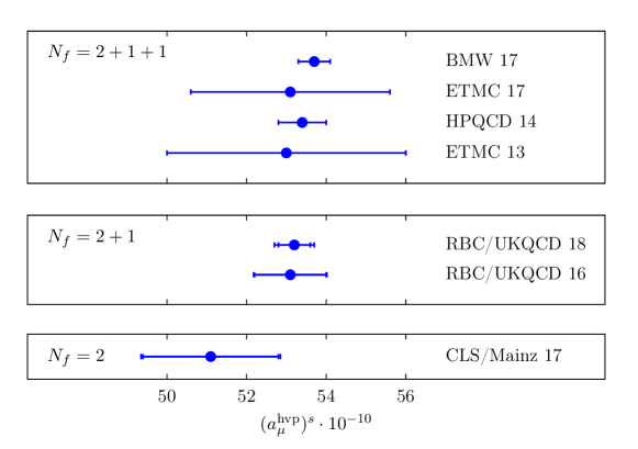
Figure 15: The hadronic vacuum polarisation contribution from the strange quark in units of $10^{-10}$. References for individual calculations are listed in Table 4.

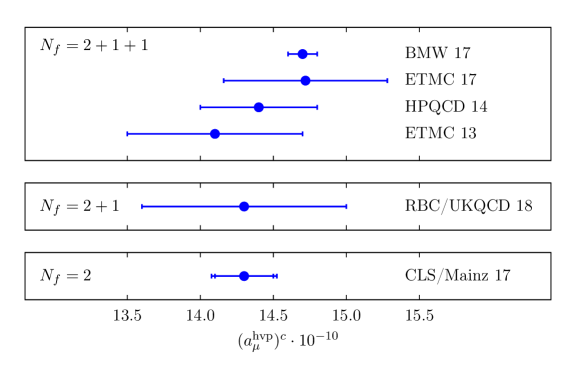
Figure 16: The hadronic vacuum polarisation contribution from the charm quark in units of $10^{-10}$. References for individual calculations are listed in Table 4.

An alternative method for determining $a_{\mu}^{\rm hvp}$ from a combination of the experimentally measured $R$-ratio and lattice data was used by RBC/UKQCD [66]. It is based on the relation between the vector correlator $G(x_{0})$ and the hadronic cross section ratio $R(s)$ derived in Ref. [94], i.e.

$$G(x_{0})=\frac{1}{12\pi^{2}}\int_{0}^{\infty}d(\sqrt{s})\,R(s)s\,e^{-\sqrt{s}x_{0}},$$ (117)

with $R(s)$ defined in Eq. (7). When multiplied by the kernel function $w(x_{0})$ of the time-momentum representation one obtains $a_{\mu}^{\rm hvp}$ via Eq. (26). As explained in detail in [165, 66], replacing the lattice determination of the vector correlator $G(x_{0})$ by the expression in Eq. (117) results in a statistically more precise integrand $w(x_{0})G(x_{0})$ for $x_{0}\lesssim 0.4$ fm and $x_{0}\gtrsim 1.0$ fm. Replacing $G(x_{0})$ by its representation in terms of the $R$-ratio for $x_{0}\leq 0.4$ fm reduces the influence from discretisation errors, while for $x_{0}\geq 1.0$ fm the uncertainties associated with the modelling of the long-distance behaviour can be eliminated. By splitting the integration over $x_{0}$ into three intervals and using the lattice data for $G(x_{0})$ only for $0.4\,{\rm{fm}}\leq x_{0}\leq 1.0$ fm, RBC/UKQCD 18 obtain

$$a_{\mu}^{\rm hvp}=(692.5\pm 2.7)\cdot 10^{-10},$$ (118)

where statistical and systematic errors from the lattice calculation and the $R$-ratio have been combined in quadrature. This estimate, shown in the lower panel of Figure 14, not only agrees very well with the results from the most recent phenomenological analyses [10, 17, 18], but is also slightly more precise. Owing to the use of the experimentally determined $R$-ratio and keeping in mind that the value of $a_{\mu}^{\rm hvp}$ is dominated by the low-energy regime, it is not too surprising that this method produces a central value that agrees so well with dispersion theory.

Collaboration	$\phantom{0.0}\Pi_{1}[{\rm{GeV}}^{-2}]$	$\phantom{-0.}\Pi_{2}[{\rm{GeV}}^{-4}]$	Comments
$N_{\rm f}=2+1+1:$
BMW 16 [61]	$0.0999(10)(9)(23)_{\rm FV}\,(13)_{\rm IB}$	$-0.181(6)(4)(10)_{\rm FV}\,(2)_{\rm IB}$	Continuum limit
	$0.0889(16)$	$-0.206(10)$	$a=0.15\,{\rm{fm}}$
HPQCD 16 [60]	$0.0892(14)$	$-0.204(9)$	$a=0.12\,{\rm{fm}}$
$N_{\rm f}=2:$
CLS/Mainz 17 [62]	$0.0883(59)$		Continuum limit
Benayoun
et al. $16\qquad$ [127, 61]	$0.0990(7)$	$-0.2057(16)$	$R(e^{+}e^{-}\to\hbox{hadrons})$

Table 6: Results for the first two time moments of the hadronic vacuum polarisation function $\hat{\Pi}(Q^{2})$. Lattice estimates have been computed at or extrapolated to the physical pion mass. The subscript “FV” on the results from [61] indicates the uncertainty in the applied volume correction, while the label “IB” denotes a phenomenological estimate of isospin breaking corrections.

Instead of focussing directly on $a_{\mu}^{\rm hvp}$ it is also instructive to discuss the individual time moments which also provide useful information, since they can be linked to the rapidly converging expansion of $a_{\mu}^{\rm hvp}$ in terms of the Mellin moments discussed in Section 2.2.6. Results for the leading two time moments published by BMW [61] are listed in Table 6 together with the estimates by HPQCD [60] and CLS/Mainz [62].

BMW correct their results for finite-volume effects, computed in chiral effective theory at one loop. They quote corrections of 2% and 10% for $\Pi_{1}$ and $\Pi_{2}$, respectively. They also add an uncertainty reflecting the fact that their results are not corrected for isospin breaking effects. HPQCD apply a correction for finite-volume effects and effects relating to the breaking of taste symmetry, which amounts to 7% for $\Pi_{1}$. The results from CLS/Mainz have been extrapolated to the continuum limit without applying any finite-volume corrections. While the estimates for $\Pi_{1}$ determined by HPQCD and CLS/Mainz agree within errors, the result from BMW is larger by 10%. A similar observation applies to $\Pi_{2}$. It is instructive to compare these findings to a recent study [127] in which the moments are determined from the experimentally determined $R$-ratio. While the phenomenological estimate for $\Pi_{1}$ agrees well with the determination from BMW, $\Pi_{2}$ from [127] compares more favourably to the estimate by HPQCD. Obviously, the current situation calls for further investigations into the systematics of lattice calculations, even more so since both BMW and HPQCD employ staggered fermions as their discretisation of the quark action. It should also be noted that the overall precision of the phenomenological determination of the moments is higher than that of current lattice calculations.

2.9 Concluding remarks on the hadronic vacuum polarisation

Recent years have seen enormous progress concerning a first-principles determination of the O($\alpha^{2}$) hadronic vacuum polarisation contribution. Lattice QCD is not only capable of providing direct determinations of $a_{\mu}^{\rm hvp}$, but also provides estimates that combine experimental information and/or other theoretical methods with lattice results. In addition to controlling the standard systematic effects arising in any lattice calculation, isospin breaking corrections, contributions from quark-disconnected diagrams, finite-volume corrections and the contributions from the IR regime must all be quantified at the desired level of precision if lattice QCD is to have a decisive impact on understanding the observed discrepancy between experiment and SM prediction. The currently available direct determinations of $a_{\mu}^{\rm hvp}$ carry an overall uncertainty of $2-3$% which is not yet sufficient to discriminate between the dispersive estimate and the “no new physics” scenario which assumes that the observed discrepancy is due to some unknown or uncontrolled hadronic effect. Ongoing efforts to provide more precise lattice QCD estimates focus on increasing the overall statistical precision, including the accuracy of the lattice scale which is a limiting factor, as well as constraining finite-volume effects and the deep IR region of the vector correlator.

3 Hadronic light-by-light scattering in $(g-2)_{\mu}$

At O($\alpha^{3}$), the theoretically most challenging hadronic contribution to $(g-2)_{\mu}$ is the scattering of light by light via QCD degrees of freedom. In this section we review the progress made in formulating the calculation of $a_{\mu}^{\rm hlbl}$ for a lattice QCD treatment, the first numerical results and discuss some of the sources of systematic error. The first proposal to compute $a_{\mu}^{\rm hlbl}$ in lattice QCD was made in 2005 [166], but this activity picked up momentum only about five years ago. Prior to that, the only approach pursued to estimate $a_{\mu}^{\rm hlbl}$ was the use of a model mainly based on the exchange of hadronic resonances with various quantum numbers (mainly $J^{PC}=0^{-+}$, $0^{++}$, $1^{++}$, $2^{++}$). In addition to the “Glasgow consensus” value $a_{\mu}^{\rm hlbl}=(105\pm 26)\cdot 10^{-11}$ quoted in Table 1, an alternative estimate is $a_{\mu}^{\rm hlbl}=(102\pm 39)\cdot 10^{-11}$ [167]. The largest contribution by far comes from the exchange of the lightest pseudoscalar mesons, $\pi^{0}$, $\eta$ and $\eta^{\prime}$. In recent years, major progress has also been made in developing a dispersive approach to $a_{\mu}^{\rm hlbl}$ [34, 35, 36, 37, 38].

3.1 General considerations

We begin with a review of the initial steps in setting up the calculation; most of this material is standard and has been known for a long time. We follow the treatment given in [30], with the difference that we work directly in the Euclidean theory. This approach is appropriate because we want to compute an electromagnetic form factor at an (infinitesimal) spacelike momentum transfer. It is well known in the lattice community that the calculation of spacelike form factors can be formulated directly in Euclidean space [168], thus making them accessible to lattice QCD simulations. Let

$$J_{\rho}={\textstyle\frac{2}{3}}\bar{u}\gamma_{\rho}u-{\textstyle\frac{1}{3}}\bar{d}\gamma_{\rho}d-{\textstyle\frac{1}{3}}\bar{s}\gamma_{\rho}s$$ (119)

be the contribution of the light quarks to the electromagnetic current (in units of $-e$, $e$ being the electric charge of the electron). Here we are interested in the matrix element of $J_{\rho}$ between single-muon states, $\langle\mu^{-}(p^{\prime},s^{\prime})|J_{\rho}(0)|\mu^{-}(p,s)\rangle$. In Euclidean space, we therefore set

$$p_{\mu}=(iE_{\boldsymbol{p}},\boldsymbol{p}),\qquad\quad p^{\prime}_{\mu}=(iE_{\boldsymbol{p}^{\prime}},\boldsymbol{p}^{\prime}),\qquad\quad k_{\mu}=p_{\mu}^{\prime}-p_{\mu}.$$ (120)

Lorentz symmetry implies generically

$$\Big{\langle}\mu^{-}(p^{\prime},s^{\prime})\big{|}J_{\rho}(0)\big{|}\,\mu^{-}(p,s)\Big{>}=-\bar{u}^{s^{\prime}}(p^{\prime})\Big{[}\gamma_{\rho}\hat{F}_{1}(k^{2})+\frac{\sigma_{\rho\tau}k_{\tau}}{2m}\hat{F}_{2}(k^{2})\Big{]}u^{s}(p),$$ (121)

with $\sigma_{\rho\tau}\equiv\frac{i}{2}\left[\gamma_{\rho},\gamma_{\tau}\right]$ in terms of the Euclidean Dirac matrices, $\left\{\gamma_{\rho},\gamma_{\sigma}\right\}=2\delta_{\rho\sigma}$. The matrix element is thus parameterised in terms of contributions (indicated by the hat) to the Dirac form factor $F_{1}(k^{2})$ and the Pauli form factor $F_{2}(k^{2})$ of the muon. The spinors $u^{s}(p)$ are the usual plane-wave solutions to the Dirac equation.

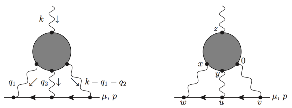
Figure 17: The hadronic light-by-light contribution to $(g-2)_{\mu}$.

Using the Feynman rules for QED in Euclidean space (see the left panel of Fig. 17), we get for the leading contribution in powers of $e$ to the matrix element

$$(ie)\Big{\langle}\mu^{-}(p^{\prime})\big{|}J_{\rho}(0)\big{|}\,\mu^{-}(p)\Big{>} = (-ie)^{3}\,(ie)^{4}\int\frac{d^{4}q_{1}}{(2\pi)^{4}}\int\frac{d^{4}q_{2}}{(2\pi)^{4}}\frac{1}{q_{1}^{2}q_{2}^{2}(q_{1}+q_{2}-k)^{2}}\cdot$$

$$\cdot\;\frac{-1}{(p^{\prime}-q_{1})^{2}+m^{2}}\,\frac{-1}{(p^{\prime}-q_{1}-q_{2})^{2}+m^{2}}\cdot\phantom{\frac{1}{1}}$$

$$\cdot\;\bar{u}(p^{\prime})\gamma^{\mu}(ip\!\!\!/^{\prime}-iq\!\!\!/{}_{1}-m)\gamma^{\nu}(ip\!\!\!/^{\prime}-iq\!\!\!/{}_{1}-iq\!\!\!/{}_{2}-m)\gamma^{\lambda}u(p)\cdot$$

$$\cdot\;\Pi_{\mu\nu\lambda\rho}(q_{1},q_{2},k-q_{1}-q_{2}),$$

with

$$\Pi_{\mu\nu\lambda\rho}(q_{1},q_{2},q_{3})=\int d^{4}x_{1}\int d^{4}x_{2}\int d^{4}x_{3}\;{\rm{e}}^{-i(q_{1}x_{1}+q_{2}x_{2}+q_{3}x_{3})}\Big{\langle}J_{\mu}(x_{1})J_{\nu}(x_{2})J_{\lambda}(x_{3})J_{\rho}(0)\Big{\rangle}_{\rm QCD}.$$ (123)

The tensor $\Pi_{\mu\nu\lambda\rho}$ satisfies

$$(q_{1})_{\mu}\,\Pi_{\mu\nu\lambda\rho}(q_{1},q_{2},q_{3})=0, (q_{2})_{\nu}\,\Pi_{\mu\nu\lambda\rho}(q_{1},q_{2},q_{3})=0,$$ (124)

$$(q_{3})_{\lambda}\,\Pi_{\mu\nu\lambda\rho}(q_{1},q_{2},q_{3})=0, (q_{1}+q_{2}+q_{3})_{\rho}\,\Pi_{\mu\nu\lambda\rho}(q_{1},q_{2},q_{3})=0.$$ (125)

The last equation implies in particular

$$k_{\sigma}\;\Pi_{\mu\nu\lambda\sigma}(q_{1},q_{2},k-q_{1}-q_{2})=0\qquad\forall k,$$ (126)

and therefore

$$\frac{\partial}{\partial k_{\rho}}\Big{(}k_{\sigma}\;\Pi_{\mu\nu\lambda\sigma}(q_{1},q_{2},k-q_{1}-q_{2})\Big{)}=0,$$ (127)

implying

$$\Pi_{\mu\nu\lambda\rho}(q_{1},q_{2},k-q_{1}-q_{2})=-k_{\sigma}\frac{\partial}{\partial k_{\rho}}\Pi_{\mu\nu\lambda\sigma}(q_{1},q_{2},k-q_{1}-q_{2}).$$ (128)

We can therefore write

$$\Big{\langle}\mu^{-}(p^{\prime},s^{\prime})\big{|}J_{\rho}(0)\big{|}\,\mu^{-}(p,s)\Big{>}=k_{\sigma}\hat{\gamma}_{\rho\sigma}^{s^{\prime}s}(p^{\prime},p),\qquad\hat{\gamma}_{\rho\sigma}^{s^{\prime}s}(p^{\prime},p)=\bar{u}^{s^{\prime}}(p^{\prime})\Gamma_{\rho\sigma}(p^{\prime},p)u^{s}(p)$$ (129)

with

$$\Gamma_{\rho\sigma}(p^{\prime},p) = -e^{6}\,\int\frac{d^{4}q_{1}}{(2\pi)^{4}}\int\frac{d^{4}q_{2}}{(2\pi)^{4}}\frac{1}{q_{1}^{2}q_{2}^{2}(q_{1}+q_{2}-k)^{2}}\cdot$$

$$\cdot\;\frac{1}{(p^{\prime}-q_{1})^{2}+m^{2}}\,\frac{1}{(p^{\prime}-q_{1}-q_{2})^{2}+m^{2}}\cdot\phantom{\frac{1}{1}}$$

$$\cdot\;\gamma^{\mu}(ip\!\!\!/^{\prime}-iq\!\!\!/{}_{1}-m)\gamma^{\nu}(ip\!\!\!/^{\prime}-iq\!\!\!/{}_{1}-iq\!\!\!/{}_{2}-m)\gamma^{\lambda}\cdot$$

$$\cdot\;\frac{\partial}{\partial k_{\rho}}\Pi_{\mu\nu\lambda\sigma}(q_{1},q_{2},k-q_{1}-q_{2}).$$

This expression is well known and has been the starting point for many calculations.

Note that due to the property $k_{\rho}k_{\sigma}\Gamma_{\rho\sigma}(p^{\prime},p)=0$, one finds that $\hat{F}_{1}(0)=0$. Identifying terms to linear order in $k$, we have

$$\hat{\gamma}_{\rho\tau}^{s^{\prime}s}(p,p)=-\bar{u}^{s^{\prime}}(p)\frac{\hat{F}_{2}(0)}{2m}\sigma_{\rho\tau}u^{s}(p).$$ (131)

By writing $-ip\!\!\!/+m=\sum_{s}u^{s}(p)\bar{u}^{s}(p)$ and using Eq. (131), one obtains the expression [169]

$$a_{\mu}^{\rm hlbl}=\hat{F}_{2}(0)=-\frac{i}{48m}{\rm Tr}\left\{[\gamma_{\rho},\gamma_{\tau}]\,(-ip\!\!\!/+m)\Gamma_{\rho\tau}(p,p)(-ip\!\!\!/+m)\right\}.$$ (132)

In summary, it suffices to know $\Gamma_{\rho\sigma}(p,p)$ to determine $\hat{F}_{2}(0)$. This observation is interesting, because in the loop integral (3.1), it means that the integrand is now function of three ($p,q_{1},q_{2}$) rather than four ($p,p^{\prime},q_{1},q_{2}$) momenta.

The number of relevant four-momenta can be further reduced, down to two, by realizing that $\hat{F}_{2}(0)$ is a Lorentz scalar, and therefore does not depend on the direction of the muon’s momentum. In the rest frame of the muon, its four-momentum has the form $p_{\mu}=(im,\boldsymbol{0})$. Therefore, in Euclidean space, the momentum may be parameterised as

$$p=i\,m\,\hat{\epsilon},$$ (133)

with $\epsilon\in\mathbb{R}^{4}$ a unit vector. The integrand in Eq. (3.1) projected onto the anomalous magnetic moment via Eq. (132), can therefore be averaged over the direction of $\hat{\epsilon}$,

$$\langle f(\hat{\epsilon})\rangle_{\hat{\epsilon}}\equiv\frac{1}{2\pi^{2}}\int d\Omega_{\epsilon}\;f(\hat{\epsilon}),$$ (134)

$2\pi^{2}$ being the surface of the unit-sphere embedded in four dimensions. The integrand for $a_{\mu}^{\rm hlbl}$ can thus be brought into the form

$$\hat{F}_{2}(0)=e^{6}\int\frac{d^{4}q_{1}}{(2\pi)^{4}}\int\frac{d^{4}q_{2}}{(2\pi)^{4}}\;\underbrace{{\cal K}_{\mu\nu\lambda[\rho\sigma]}(q_{1},q_{2})}_{{\displaystyle{\rm QED}}}\underbrace{\Big{[}\frac{\partial}{\partial k_{\rho}}\Pi_{\mu\nu\lambda\sigma}(q_{1},q_{2},k-q_{1}-q_{2})\Big{]}_{k=0}}_{{\displaystyle{\rm QCD}}}.$$ (135)

After the contraction of the five Lorentz indices of the QED kernel ${\cal K}_{\mu\nu\lambda\rho\sigma}$ with those of the QCD four-point function, the integrand is a Lorentz scalar. It is therefore a function of the three invariants $q_{1}^{2}$, $q_{2}^{2}$ and $q_{1}\cdot q_{2}$. Performing the integral in hyperspherical coordinates, only the integrals over these variables are non-trivial. The reduction to a three-dimensional integral can be made explicit if the QCD four-point function is decomposed into a number of tensor structures with associated form factors, which are functions of $q_{1}^{2},q_{2}^{2},q_{1}\cdot q_{2}$. This program has been carried out in [36]. Taking into account crossing symmetry, a total of twelve form factors characterizing $\frac{\partial}{\partial k_{\rho}}\Pi_{\mu\nu\lambda\sigma}(q_{1},q_{2},k-q_{1}-q_{2})_{k=0}$ contribute to $a_{\mu}^{\rm hlbl}$. From a lattice point of view, a possible strategy is thus to provide a parameterisation of each of these twelve form factors, which can then be fed into the integral over ($q_{1}^{2},q_{2}^{2},q_{1}\cdot q_{2}$) to obtain $\hat{F}_{2}(0)$. No attempt has been made yet to implement this strategy.

As will be described in Section 3.4, it is also possible to write the desired quantity in terms of a position-space integral,

$$\hat{F}_{2}(0) = \frac{me^{6}}{3}\int d^{4}y\int d^{4}x\;\underbrace{\bar{\cal L}_{[\rho,\sigma];\mu\nu\lambda}(x,y)}_{{\displaystyle{\rm QED}}}\;\underbrace{i\widehat{\Pi}_{\rho;\mu\nu\lambda\sigma}(x,y)}_{{\displaystyle{\rm QCD}}}\;,$$ (136)

$$i\widehat{\Pi}_{\rho;\mu\nu\lambda\sigma}(x,y) = -\int d^{4}z\;z_{\rho}\,\Big{\langle}\,J_{\mu}(x)\,J_{\nu}(y)\,J_{\sigma}(z)\,J_{\lambda}(0)\Big{\rangle}.$$ (137)

From the point of view of lattice calculations, one advantage of this representation is that for fixed $y$, the $x$-integral over the fully connected contribution to the four-point function can be evaluated with a computational effort of order volume by using the technique of sequential propagators – see the next paragraph. An explicit decomposition of the QCD four-point function into form factors is thus not necessary. After the $x$-integral is performed, by Lorentz invariance of $a_{\mu}^{\rm hlbl}$, the $y$ integral reduces to a one-dimensional integral over $|y|$. A second advantage is that on the torus, the asymptotic finite-size effects are determined by the longest QCD correlation length; power-law corrections in the box size $L$ are thus avoided altogether.

The HLbL scattering amplitude, which is determined by the four-point function (123) of the vector current, can be computed in lattice QCD by constructing all possible Wick contractions of the quark fields – their interaction with the SU(3) gauge fields being taken into account non-perturbatively by the importance-sampling of the gauge fields. A complete list of the Wick contraction topology classes is given in Fig. 18. Each class consists of a number of Wick contractions; for the fully connected class, labelled “(4)” in Fig. 18, there are six of them. An important computational aspect in lattice QCD is then the following: consider an $n$-point correlation function of the type

$$\sum_{x_{2}}f(x_{2})\;\left\langle{\cal O}_{0}(0)\,{\cal O}_{1}(x_{1})\,{\cal O}_{2}(x_{2})\right\rangle,$$ (138)

with ${\cal O}_{i}(x)=\bar{\psi}(x)\Gamma_{i}\psi(x)$. One of the fully connected contributions to the Wick contractions reads

$$\sum_{x_{2}}f(x_{2})\;\left\langle\Gamma_{0}S^{f}(0,x_{1})\Gamma_{1}S^{f}(x_{1},x_{2})\Gamma_{2}S^{f}(x_{2},0)\right\rangle,$$ (139)

where $S^{f}$ is the quark propagator of flavour $f$ and the average is taken over the SU(3) gauge field. The key to computing the quantity

$$v(x_{1})\equiv\sum_{x_{2}}f(x_{2})S^{f}(x_{1},x_{2})\Gamma_{2}S^{f}(x_{2},0)$$ (140)

is to note that it satisfies

$$\sum_{z}D^{f}(x,z)v(z)=f(x)\Gamma_{2}S^{f}(x,0).$$ (141)

Thus the spinor field $v(z)$, called a sequential propagator, is obtained by inverting the Dirac operator on a single given “source” field, $D^{f}v=\eta$, with $\eta(x)=f(x)\Gamma_{2}S^{f}(x,0)$. This technique allows one to calculate the correlation function (138) with O($V$) operations. More generally, correlation functions of the type

$$C[f_{1},\dots,f_{n-1}](x_{n})=\sum_{x_{1},\dots,x_{n-1}}\Big{(}\prod_{i=1}^{n-1}f_{i}(x_{i})\Big{)}\;\langle{\cal O}_{1}(x_{1})\dots\cal O_{n}(x_{n})\rangle$$ (142)

can be computed simultaneously for all $x_{n}$ with O($V$) operations using this technique. The important point is that the weighting function of the coordinates $(x_{1},\dots,x_{n-1})$ must be factorised, $\prod_{i=1}^{n-1}f_{i}(x_{i})$. This observation will be used repeatedly in the forthcoming sections, particularly for computing the fully connected class of Wick contractions of the vector four-point function.

Figure 18: The five classes of quark-field Wick contractions contributing to HLbL scattering. From left to right we refer to them as (4), (2,2), (3,1), (2,1,1) and (1,1,1,1). Each class contains a number of actual contractions. Figure from [170].

3.2 Stochastic U(1) field

In this subsection we describe a class of lattice methods to compute $a_{\mu}^{\rm hlbl}$ whose common point is the (at least partially) stochastic treatment of the electromagnetic field. We follow the treatment of Ref. [171]. Consider then the Euclidean correlation function

$$-{\cal M}^{\rm l+h}_{\nu}(x_{\rm src},x_{\rm op},x_{\rm snk})=\left\langle\mu(x_{\rm snk})\;J^{\rm l+h}_{\nu}(x_{\rm op})\;\bar{\mu}(x_{\rm src})\right\rangle$$ (143)

involving the muon field $\mu(x)$ and the full electromagnetic current $J^{\rm l+h}_{\nu}(x)$ in units of $(-e)$. For $t_{\rm src}\to-\infty$ and $t_{\rm snk}\to+\infty$, the Fourier-transform of ${\cal M}_{\nu}(x_{\rm src},x_{\rm op},x_{\rm snk})$, projecting the initial-state muon on momentum $\boldsymbol{p}$ and the final-state muon on momentum $\boldsymbol{p}^{\prime}$, is proportional to the matrix element (121), a linear combination of the Dirac and Pauli form factors at momentum transfer $q=p^{\prime}-p$.

However, treating QED perturbatively, there are many Feynman diagrams contributing to ${\cal M}_{\nu}(x_{\rm src},x_{\rm op},x_{\rm snk})$, and we are only interested in the HLbL contribution. Therefore, we keep only the hadronic contribution $J_{\nu}$ of $J^{\rm l+h}_{\nu}$ and select the relevant Feynman diagrams. Call this correlation function ${\cal M}_{\nu}$ and consider the fully connected HLbL contribution ${\cal M}^{(4)}_{\nu}$,

$${\cal M}^{(4)}_{\nu}(x_{\rm src},x_{\rm op},x_{\rm snk}) = \sum_{x,y,z}{\cal F}_{\nu}(x,y,z,x_{\rm src},x_{\rm op},x_{\rm snk}),$$ (144)

$$-ie{\cal F}_{\nu}(x,y,z,x_{\rm src},x_{\rm op},x_{\rm snk}) = -(-ie)^{3}(ie)^{4}\sum_{f=u,d,s}{\cal Q}_{f}^{4}\;$$

$$\Big{\langle}{\rm Tr}\{\gamma_{\nu}S^{f}(x_{\rm op},x)\gamma_{\rho}S^{f}(x,z)\gamma_{\kappa}S^{f}(z,y)\gamma_{\sigma}S^{f}(y,x_{\rm op})\}\Big{\rangle}_{{\rm SU}(3)}$$

$$\times\sum_{x^{\prime},y^{\prime},z^{\prime}}G_{\rho\rho^{\prime}}(x,x^{\prime})G_{\sigma\sigma^{\prime}}(y,y^{\prime})G_{\kappa\kappa^{\prime}}(z,z^{\prime})\;$$

$$\Big{(}S_{0}(x_{\rm snk},x^{\prime})\gamma_{\rho^{\prime}}S_{0}(x^{\prime},z^{\prime})\gamma_{\kappa^{\prime}}S_{0}(z^{\prime},y^{\prime})\gamma_{\sigma^{\prime}}S_{0}(y^{\prime},x_{\rm src})$$

$$+S_{0}(x_{\rm snk},z^{\prime})\gamma_{\kappa^{\prime}}S_{0}(z^{\prime},x^{\prime})\gamma_{\rho^{\prime}}S_{0}(x^{\prime},y^{\prime})\gamma_{\sigma^{\prime}}S_{0}(y^{\prime},x_{\rm src})$$

$$+\textrm{four other permutations}\Big{)}.$$

Here $S^{f}(x,y)$ is the propagator of quark flavour $f$, while

$$S_{0}(x,y)=\int\frac{d^{4}p}{(2\pi)^{4}}\frac{{\rm{e}}^{ip(x-y)}}{ip_{\mu}\gamma_{\mu}+m}$$ (146)

is the free muon propagator, and $G_{\mu\mu^{\prime}}(x,y)$ is the free photon propagator. While ${\cal F}_{\nu}(x,y,z,x^{\prime},y^{\prime},z^{\prime})$ is relatively straightforward to compute for fixed values of its arguments, the exact evaluation of the six spacetime sums is computationally far too costly. Noting the identity (in Feynman gauge)

$$\int d^{4}z\int d^{4}z^{\prime}\;G_{\kappa\kappa^{\prime}}(z,z^{\prime})f_{\kappa}(z)g_{\kappa^{\prime}}(z^{\prime})=\int\frac{d^{4}k}{(2\pi)^{4}}\frac{\tilde{f}_{\kappa}(-k)\;\tilde{g}_{\kappa}(k)}{k^{2}}$$ (147)

for test functions $f(x),g(x)$ and using the shorthand notation $\int_{k}\equiv\int\frac{d^{4}k}{(2\pi)^{4}}$, we can rewrite Eq. (144) as

$${\cal M}^{(4)}_{\nu}(x_{\rm src},x_{\rm op},x_{\rm snk}) = (-ie)^{3}(ie)^{3}\sum_{f=u,d,s}{\cal Q}_{f}^{4}\;\int_{k,p,\ell}\frac{1}{k^{2}\,p^{2}\,\ell^{2}}$$ (148)

$$\bigg{(}\sum_{x,y,z}{\rm{e}}^{i(kz+\ell y+px)}\,\Big{\langle}{\rm Tr}\{\gamma_{\nu}S^{f}(x_{\rm op},x)\gamma_{\rho}S^{f}(x,z)\gamma_{\kappa}S^{f}(z,y)\gamma_{\sigma}S^{f}(y,x_{\rm op})\}\Big{\rangle}_{{\rm SU}(3)}\bigg{)}$$

$$\times\bigg{(}\sum_{x^{\prime},y^{\prime},z^{\prime}}{\rm{e}}^{-i(kz^{\prime}+\ell y^{\prime}+px^{\prime})}\Big{(}S_{0}(x_{\rm snk},x^{\prime})\gamma_{\rho}S_{0}(x^{\prime},z^{\prime})\gamma_{\kappa}S_{0}(z^{\prime},y^{\prime})\gamma_{\sigma}S_{0}(y^{\prime},x_{\rm src})$$

$$+S_{0}(x_{\rm snk},z^{\prime})\gamma_{\kappa}S_{0}(z^{\prime},x^{\prime})\gamma_{\rho}S_{0}(x^{\prime},y^{\prime})\gamma_{\sigma}S_{0}(y^{\prime},x_{\rm src})+\dots\Big{)}\bigg{)}.$$

For fixed momenta $p,\ell$, the integrand can be computed simultaneously for all $k$ with O($V$) operations. However, an expensive sampling of the momenta $p,\ell$ then remains. An exact evaluation is however not required, since the average $\langle\dots\rangle_{U}$ over the gluon degrees of freedom is performed stochastically in any case.

One way to generate ${\cal M}_{\nu}(x_{\rm src},x_{\rm op},x_{\rm snk})$ and reduce the computational burden is thus to treat two of the photon propagators stochastically. In the method proposed in [166], one considers a difference of correlation functions,

$${\cal M}^{(4)}_{\nu}(x_{\rm src},x_{\rm op},x_{\rm snk})=e^{2}\!\!\!\sum_{f=u,d,s}{\cal Q}_{f}^{2}\int_{k}\frac{1}{k^{2}}$$ (149)

$$\cdot\;\bigg{[}\Big{\langle}\sum_{z}{\rm{e}}^{ikz}\,{\rm Tr}\Big{\{}\gamma_{\nu}S^{f}(x_{\rm op},z)\gamma_{\kappa}S^{f}(z,x_{\rm op})\Big{\}}\sum_{z^{\prime}}{\rm{e}}^{-ikz^{\prime}}S(x_{\rm snk},z^{\prime})\gamma_{\kappa}S(z^{\prime},x_{\rm src})\Big{\rangle}_{{\rm SU}(3)\times{\rm U}(1)}$$

$$-\;\Big{\langle}\sum_{z}{\rm{e}}^{ikz}\,{\rm Tr}\{\gamma_{\nu}S^{f}(x_{\rm op},z)\gamma_{\kappa}S^{f}(z,x_{\rm op})\}\Big{\rangle}_{{\rm SU}(3)\times{\rm U}(1)}\cdot\sum_{z^{\prime}}{\rm{e}}^{-ikz^{\prime}}\Big{\langle}S(x_{\rm snk},z^{\prime})\gamma_{\kappa}S(z^{\prime},x_{\rm src})\Big{\rangle}_{{\rm U}(1)}$$

$$\quad+\;{\rm O}(\alpha^{3})\bigg{]}.$$

Here $S(x,y)$ is the muon propagator in a background U(1) field and $S^{f}(x,y)$ the quark propagator of flavour $q$ in a background ${\rm SU}(3)\times{\rm U}(1)$ field. The subtraction implies that only the “1-photon irreducible” graphs are kept, i.e. more than one photon must be exchanged between the muon and the QCD degrees of freedom. By charge conjugation invariance, this number must be odd; hence the first contribution involves the exchange of three photons and corresponds to the desired HLbL contribution to the amplitude ${\cal M}_{\nu}(x_{\rm src},x_{\rm op},x_{\rm snk})$. The computational cost for one configuration of ${\rm SU}(3)\times{\rm U}(1)$ gauge fields has been reduced to O($V$). At this point it remains to be determined how many samples of the fields are necessary to achieve a given accuracy on the result. Note that inside the square bracket of Eq. (149) an O$(e^{2})$ contribution cancels, leaving over an O$(e^{4})$ contribution. The latter, including the explicit $e^{2}$ factor outside the square bracket, represents the desired set of diagrams of the connected HLbL contribution (O$(e^{6})$). Proof-of-principle results obtained with this method have been presented in Ref. [69] at pion masses of 330 MeV and larger.

A different stochastic treatment of the U(1) field was proposed in [171], which avoids the large cancellation appearing in Eq. (149). It involves introducing two stochastic U(1) fields $A_{\mu}(x)$ and $B_{\mu}(x)$, such that

$$\left\langle A_{\mu}(x)\,A_{\mu^{\prime}}(y)\right\rangle_{A}=\left\langle B_{\mu}(x)\,B_{\mu^{\prime}}(y)\right\rangle_{B}=G_{\mu\mu^{\prime}}(x,y).$$ (150)

Using this equation to replace $G_{\rho\rho^{\prime}}(x,x^{\prime})$ and $G_{\sigma\sigma^{\prime}}(y,y^{\prime})$ in Eq. (3.2) by their stochastic estimates in terms of $A$ and $B$ fields respectively, one obtains

$${\cal M}^{(4)}_{\nu}(x_{\rm src},x_{\rm op},x_{\rm snk}) = e^{6}\sum_{f=u,d,s}{\cal Q}_{f}^{4}\;\int_{k}\frac{1}{k^{2}}\;\bigg{\langle}\sum_{x,y,z}A_{\rho}(x)B_{\sigma}(y)\,{\rm{e}}^{ikz}$$

$$\Big{\langle}{\rm Tr}\Big{\{}\gamma_{\nu}S^{f}(x_{\rm op},x)\gamma_{\rho}S^{f}(x,z)\gamma_{\kappa}S^{f}(z,y)\gamma_{\sigma}S^{f}(y,x_{\rm op})\Big{\}}\Big{\rangle}_{{\rm SU}(3)}$$

$$\times\sum_{x^{\prime},y^{\prime},z^{\prime}}A_{\rho^{\prime}}(x^{\prime})B_{\sigma^{\prime}}(y^{\prime})\,{\rm{e}}^{-ikz^{\prime}}$$

$$\Big{(}S_{0}(x_{\rm snk},x^{\prime})\gamma_{\rho^{\prime}}S_{0}(x^{\prime},z^{\prime})\gamma_{\kappa}S_{0}(z^{\prime},y^{\prime})\gamma_{\sigma^{\prime}}S_{0}(y^{\prime},x_{\rm src})$$

$$+S_{0}(x_{\rm snk},z^{\prime})\gamma_{\kappa}S_{0}(z^{\prime},x^{\prime})\gamma_{\rho^{\prime}}S_{0}(x^{\prime},y^{\prime})\gamma_{\sigma^{\prime}}S_{0}(y^{\prime},x_{\rm src})+\dots\Big{)}\bigg{\rangle}_{A,B}.$$

The operation just performed allows one to factorise the sums over $x,y$ from those over $x^{\prime},y^{\prime}$, so that the computational load for one instance of the $A,B$ fields becomes manageable. A concrete prescription for the generation of the stochastic U(1) field satisfying Eq. (150) is given in [171].

3.3 Sampling the positions of QED vertices

As the reader may have noted, the methods discussed so far allow for the determination of the full form factors $\hat{F}_{1}(q^{2})$ and $\hat{F}_{2}(q^{2})$, when in fact for $(g-2)_{\mu}$ all that is needed is $\hat{F}_{2}(0)$. It is then natural to ask whether the computational cost can be reduced if one is interested only in one value of the momentum transfer.

We therefore return to Eq. (148). From the definition (143), an important observation is that if $x_{\rm src}$ and $x_{\rm snk}$ are projected on definite spatial momenta $\boldsymbol{p}$ and $\boldsymbol{p}^{\prime}$, and $|t_{\rm snk}-t_{\rm src}|\to\infty$, the dependence of ${\cal M}_{\nu}(x_{\rm src},x_{\rm op},x_{\rm snk})$ on the insertion point $x_{\rm op}$ of the electromagnetic current is completely determined by four-momentum conservation, since the correlation function is then saturated by the muon. Following [171], we re-use expression (3.2) and define

$${\cal F}_{\nu}(\boldsymbol{q},x,y,z,x_{\rm op}) = \lim_{\begin{subarray}{c}t_{\rm src}\to-\infty\\ t_{\rm snk}\to+\infty\end{subarray}}{\rm{e}}^{E_{\boldsymbol{p}}(t_{\rm op}-t_{\rm src})+E_{\boldsymbol{p}^{\,\prime}}(t_{\rm snk}-t_{\rm op})}\!\!\sum_{x_{\rm snk},x_{\rm src}}\!\!{\rm{e}}^{-i\boldsymbol{q}\cdot(x_{\rm src}+x_{\rm snk})/2}\;\cdot$$

$$\qquad\qquad\qquad\qquad\qquad\cdot\;{\cal F}_{\nu}(x,y,z,x_{\rm op},x_{\rm snk},x_{\rm op}),$$

$${\cal M}_{\nu}(\boldsymbol{q}) = {\rm{e}}^{i\boldsymbol{q}\cdot{\boldsymbol{x}}_{\rm op}}\sum_{x,y,z}{\cal F}_{\nu}(\boldsymbol{q},x,y,z,x_{\rm op}).$$ (153)

The quantity ${\cal M}_{\nu}(\boldsymbol{q})$ does not depend on $x_{\rm op}$, and ${\rm{e}}^{i\boldsymbol{q}\cdot{\boldsymbol{x}}_{\rm op}}{\cal F}_{\nu}(\boldsymbol{q},x,y,z,x_{\rm op})$ is invariant under a common shift to the position-space vectors ($x,y,z,x_{\rm op}$). Based on these observations, one can choose the average of $x$ and $y$ to coincide with the origin and write

$${\cal M}_{\nu}(\boldsymbol{q})=\sum_{r,z,x_{\rm op}}{\rm{e}}^{i\boldsymbol{q}\cdot\boldsymbol{x}_{\rm op}}\;{\cal F}_{\nu}(\boldsymbol{q},r/2,-r/2,z,x_{\rm op}).$$ (154)

Explicitly, after a few rearrangements the matrix element can be brought into the form

$${\cal M}_{\nu}(\boldsymbol{q})=e^{6}\sum_{f=u,d,s}{\cal Q}_{f}^{4}\;\sum_{r}{\cal G}_{\rho\sigma\kappa}(r,\boldsymbol{p},\boldsymbol{q})$$

$$\sum_{z,x_{\rm op}}{\rm{e}}^{i\boldsymbol{q}\cdot\boldsymbol{x}_{\rm op}+(E_{\boldsymbol{p}}-E_{\boldsymbol{p}^{\,\prime}})t_{\rm op}}\;\Big{\langle}{\rm Tr}\Big{\{}\gamma_{\nu}S^{f}(x_{\rm op},r/2)\gamma_{\rho}S^{f}(r/2,z)\gamma_{\kappa}S^{f}(z,-r/2)\gamma_{\sigma}S^{f}(-r/2,x_{\rm op})\Big{\}}\Big{\rangle}_{{\rm SU}(3)},$$

$${\cal G}_{\rho\sigma\kappa}(r,\boldsymbol{p},\boldsymbol{q})=\sum_{x^{\prime},y^{\prime},z^{\prime}}G_{\kappa\kappa^{\prime}}(z,z^{\prime})\;G_{\rho\rho^{\prime}}(r/2,x^{\prime})\;G_{\sigma\sigma^{\prime}}(-r/2,y^{\prime})$$ (155)

$$\lim_{\begin{subarray}{c}t_{\rm src}\to-\infty\\ t_{\rm snk}\to+\infty\end{subarray}}\sum_{\boldsymbol{x}_{\rm snk},\boldsymbol{x}_{\rm src}}{\rm{e}}^{i\boldsymbol{p}\cdot\boldsymbol{x}_{\rm src}-E_{\boldsymbol{p}}t_{\rm src}-i\boldsymbol{p}^{\,\prime}\cdot\boldsymbol{x}_{\rm snk}+E_{\boldsymbol{p}^{\,\prime}}t_{\rm snk}}\;\Big{(}S_{0}(x_{\rm snk},x^{\prime})\gamma_{\rho^{\prime}}S_{0}(x^{\prime},z^{\prime})\gamma_{\kappa^{\prime}}S_{0}(z^{\prime},y^{\prime})\gamma_{\sigma^{\prime}}S_{0}(y^{\prime},x_{\rm src})$$

$$\qquad\qquad\qquad\qquad\qquad\qquad\quad+S_{0}(x_{\rm snk},z^{\prime})\gamma_{\kappa^{\prime}}S_{0}(z^{\prime},x^{\prime})\gamma_{\rho^{\prime}}S_{0}(x^{\prime},y^{\prime})\gamma_{\sigma^{\prime}}S_{0}(y^{\prime},x_{\rm src})+\dots\Big{)}.$$

We note that in the latter form, the second line can, for fixed $(r,\boldsymbol{p},\boldsymbol{q})$, be evaluated for all $z$ and $x_{\rm op}$ with O($V$) operations, by setting point sources at $r/2$ and at $-r/2$. The object ${\cal G}_{\rho\sigma\kappa}(r,\boldsymbol{p},\boldsymbol{q})$, which contains only photon and muon propagators, can also be evaluated with O($V$) operations. This QED part can of course be simplified further, but we will not go into further details. The important point is that, after the limit $\boldsymbol{q}\to 0$ is taken, the sum over the four-vector $r$ remains to be done. The authors of [171] have developed a stochastic integration technique to perform this task, sampling the short distances more finely that the longer distances.

A test of the method for the contribution of a free quark-loop to $a_{\mu}^{\rm hlbl}$ was performed in Ref. [171], see Fig. 19. The known result in the continuum and infinite-volume limits is reproduced with a statistical precision below one percent, with the dominant systematic uncertainty coming from the linear extrapolation to infinite-volume in the variable $1/L^{2}$. This method was found to be more efficient than the use of stochastic U(1) fields, for reasons that are largely understood [171], even though within the latter class of methods the treatment based on Eq. (3.2) represented a significant improvement over the older method based on Eq. (149).

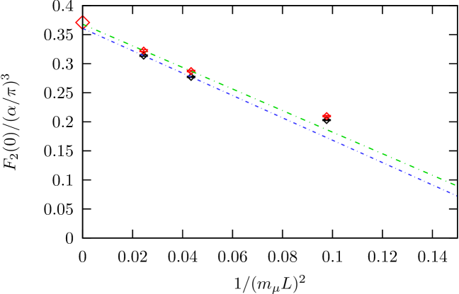
Figure 19: Study of finite-size effects for lattice calculations of $a_{\mu}^{\rm hlbl}$ [171]: extrapolation to infinite volume of the free-fermion-loop contribution to $a_{\mu}^{\rm LbL}$ computed on a torus of dimension $L\times L\times L$ using the method described in Section 3.3.

3.4 Semi-analytic calculation of the QED kernel

Position-space methods are often advantageous in lattice QCD, because the elementary degrees of freedom are treated in position space (quark fields $\psi(x)$ and gauge variables $U_{\mu}(x)$), rather than in momentum space. Moreover, using position-space perturbation theory for the photons and leptons in infinite volume eliminates the power-law corrections in the volume that one incurs when treating the U(1) gauge field on the torus. See [148] for an alternative idea to avoid the power-law corrections. Below we follow the treatment presented in [172, 173, 174, 175]. A similar treatment was developed in [176], to which we return at the end of this subsection.

One may start from Eqs. (3.1) and (132), which hold in the infinite-volume, continuum theory. Interchanging the order of the integrations and expressing the $q_{1}$ and $q_{2}$ integrals in terms of position-space propagators, one arrives at [173]

$$\Gamma_{\rho\sigma}(p,p) = -e^{6}\int_{x_{1},x_{2}}K_{\mu\nu\lambda}(x_{1},x_{2},p)\;\widehat{\Pi}_{\rho;\mu\nu\lambda\sigma}(x_{1},x_{2}),$$ (156)

$$\widehat{\Pi}_{\rho;\mu\nu\lambda\sigma}(x_{1},x_{2}) = \int_{x_{3}}(+ix_{3})_{\rho}\,\Big{\langle}\,J_{\mu}(x_{1})\,J_{\nu}(x_{2})\,J_{\sigma}(x_{3})\,J_{\lambda}(0)\Big{\rangle},$$ (157)

with the shorthand notation $\int_{x}\equiv\int d^{4}x$ for position-space integrals and

$$K_{\mu\nu\lambda}(x_{1},x_{2},p) = \gamma_{\mu}(ip\!\!\!/+\partial\!\!\!/^{(x_{1})}-m)\gamma_{\nu}(ip\!\!\!/+\partial\!\!\!/^{(x_{1})}+\partial\!\!\!/^{(x_{2})}-m)\gamma_{\lambda}\;{\cal I}(\hat{\epsilon},x_{1},x_{2}),\phantom{\frac{1}{1}}$$ (158)

$${\cal I}(\hat{\epsilon},x,y) = \int_{q,k}\frac{1}{q^{2}k^{2}(q+k)^{2}}\frac{1}{(p-q)^{2}+m^{2}}\frac{1}{(p-q-k)^{2}+m^{2}}{\rm{e}}^{-i(qx+ky)}.$$ (159)

We remind the reader that the unit vector $\hat{\epsilon}$ parameterises the momentum of the muon, $p=i\,m\,\hat{\epsilon}$. An important point is that the scalar function ${\cal I}$ requires infrared regularisation, which however can be dropped after the derivatives are applied to it to compute $K_{\mu\nu\lambda}(x,y)$.

Combining Eqs. (156) and (132), one arrives at an expression of the form [172]

$$\hat{F}_{2}(0)=\frac{me^{6}}{3}\int_{x,y}{\cal L}_{[\rho,\sigma];\mu\nu\lambda}(\hat{\epsilon},x,y)\;i\widehat{\Pi}_{\rho;\mu\nu\lambda\sigma}(x,y).$$ (160)

Exploiting the fact that $\hat{F}_{2}(0)$ is a Lorentz scalar, we may average the right-hand side over the direction of the muon’s momentum, so that [172]

$$\hat{F}_{2}(0)=\frac{me^{6}}{3}\int_{x,y}\bar{\cal L}_{[\rho,\sigma];\mu\nu\lambda}(x,y)\;i\widehat{\Pi}_{\rho;\mu\nu\lambda\sigma}(x,y),\quad\bar{\cal L}_{[\rho,\sigma];\mu\nu\lambda}(x,y)=\Big{\langle}{\cal L}_{[\rho,\sigma];\mu\nu\lambda}(\hat{\epsilon},x,y)\Big{\rangle}_{\hat{\epsilon}}.\quad\quad\quad$$ (161)

The calculation of the kernel proceeds as follows. The kernel is written as

$$\bar{\cal L}_{[\rho,\sigma];\mu\nu\lambda}(x,y) = \sum_{A={\rm I,II,III}}{\cal G}^{A}_{\delta[\rho\sigma]\mu\alpha\nu\beta\lambda}T^{(A)}_{\alpha\beta\delta}(x,y).$$ (162)

The ${\cal G}^{A}_{\delta[\rho\sigma]\mu\alpha\nu\beta\lambda}$ are sums of products of Kronecker deltas resulting from traces of Dirac matrices. The rank-three tensor $T^{(A)}_{\alpha\beta\delta}(x,y)$ can be written in terms of a scalar, a vector and a tensor component of ${\cal I}(\hat{\epsilon},x,y)$ viewed as a function of the unit vector $\hat{\epsilon}$,

$$T^{({\rm I})}_{\alpha\beta\delta}(x,y) = \partial^{(x)}_{\alpha}(\partial^{(x)}_{\beta}+\partial^{(y)}_{\beta})V_{\delta}(x,y),$$ (163)

$$T^{({\rm II})}_{\alpha\beta\delta}(x,y) = m\,\partial^{(x)}_{\alpha}\Big{(}T_{\beta\delta}(x,y)+\frac{1}{4}\delta_{\beta\delta}S(x,y)\Big{)}$$ (164)

$$T^{({\rm III})}_{\alpha\beta\delta}(x,y) = m\,(\partial^{(x)}_{\beta}+\partial^{(y)}_{\beta})\Big{(}T_{\alpha\delta}(x,y)+\frac{1}{4}\delta_{\alpha\delta}S(x,y)\Big{)},$$ (165)

with

$$S(x,y)=\Big{\langle}{\cal I}\Big{\rangle}_{\hat{\epsilon}},\qquad V_{\delta}(x,y)=\Big{\langle}\hat{\epsilon}_{\delta}{\cal I}\Big{\rangle}_{\hat{\epsilon}},\qquad T_{\beta\delta}(x,y)=\Big{\langle}\Big{(}\hat{\epsilon}_{\delta}\hat{\epsilon}_{\beta}-{\textstyle\frac{1}{4}}\delta_{\beta\delta}\Big{)}\;{\cal I}\Big{\rangle}_{\hat{\epsilon}}.$$ (166)

Only the scalar contribution $S(x,y)$ contains the infrared divergence of ${\cal I}(\hat{\epsilon},x,y)$; the divergence cancels after the derivatives in (164) and (165) are applied. In the intermediate steps of the calculation, it can for instance be regulated by introducing a photon mass. The vector and tensor functions are parameterised by, respectively, two and three weight functions,

$$S(x,y) \!\!=\!\! \bar{g}^{(0)}(|x|,x\cdot y,|y|),\phantom{\frac{1}{1}}$$ (167)

$$V_{\delta}(x,y) \!\!=\!\! x_{\delta}\bar{\mathfrak{g}}^{(1)}(|x|,x\cdot y,|y|)+y_{\delta}\bar{\mathfrak{g}}^{(2)}(|x|,x\cdot y,|y|),$$ (168)

$$T_{\alpha\beta}(x,y) \!\!=\!\! \left(x_{\alpha}x_{\beta}-{\textstyle\frac{1}{4}}x^{2}\,\delta_{\alpha\beta}\right)\;\bar{\mathfrak{l}}^{(1)}+\left(y_{\alpha}y_{\beta}-{\textstyle\frac{1}{4}}y^{2}\,\delta_{\alpha\beta}\right)\;\bar{\mathfrak{l}}^{(2)}+\left(x_{\alpha}y_{\beta}+y_{\alpha}x_{\beta}-{\textstyle\frac{1}{2}}x\cdot y\,\delta_{\alpha\beta}\right)\;\bar{\mathfrak{l}}^{(3)}.\qquad$$ (169)

In total, the QED kernel $\bar{\cal L}_{[\rho,\sigma];\mu\nu\lambda}(x,y)$ is thus parameterised by six weight functions $\bar{g}^{(0)}$, $\bar{\mathfrak{g}}^{(1)}$, $\bar{\mathfrak{g}}^{(2)}$, $\bar{\mathfrak{l}}^{(1)}$, $\bar{\mathfrak{l}}^{(2)}$ and $\bar{\mathfrak{l}}^{(3)}$, which are functions of $(x^{2},y^{2},x\cdot y)$. The averaging over $\hat{\epsilon}$ is performed analytically [173] using the Gegenbauer polynomial technique, which is the four-dimensional analogue of applying Legendre polynomials to three-dimensional problems; see for instance [30]. In the final step, the calculation of the form factors involves a two-dimensional numerical integration of a function defined by an infinite series. Through the use of Lorentz covariance, the calculation of the kernel thus involves a manageable amount of computation and storage.

In the course of an actual lattice calculation, the six form factors can be read in and combined into ${\cal L}_{[\rho,\sigma];\mu\nu\lambda}(x,y)$ “on the fly” for fixed $y$ [173]. In analytic calculations, once all indices of ${\cal L}_{[\rho,\sigma];\mu\nu\lambda}(x,y)$ are contracted with $\widehat{\Pi}_{\rho;\mu\nu\lambda\sigma}(x,y)$, the eight-dimensional integral over $(x,y)$ reduces to a three-dimensional integral over $(x^{2},y^{2},\hat{x}\cdot\hat{y})$. However, in practical lattice calculations, the sum over $x$ can be carried out explicitly using the sequential-propagator technique with O($V$) operations and no significant increase in computational cost. After the $x$ integral is carried out, by Lorentz invariance of $a_{\mu}^{\rm hlbl}$, the $y$ integral collapses to a one-dimensional integral, $\int d^{4}y\to 2\pi^{2}\int_{0}^{\infty}d|y|\;|y|^{3}$. For that reason, one may expect that the number of $y$ points at which the integrand needs to be evaluated is manageable [172], perhaps of order twenty.

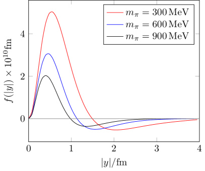
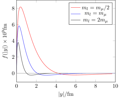
Figure 20: The integrand to obtain the $\pi^{0}$ pole (left) and the lepton loop (right) contribution to $a_{\mu}^{\rm hlbl}$ in infinite-volume position space based on Eq. (161). The vector-dominance model was used for the pion transition form factor. The known results are reproduced at the percent level. Figures from [175].

To demonstrate the validity of the position-space approach described above, the $\pi^{0}$ contribution to $a_{\mu}^{\rm hlbl}$ was computed [173, 174] in infinite volume and shown to reproduce the result obtained using momentum-space methods; see Fig. 20. Similarly, the analytically known contribution of a free quark was reproduced [174] at the one-percent level. In the latter case, a closed analytic expression was obtained for $\widehat{\Pi}_{\rho;\mu\nu\lambda\sigma}(x,y)$.

As noted at the beginning of this subsection, a closely related approach has been implemented and tested on the lattice using a free quark loop [176]. In the latter publication, however, the muon rest frame was chosen and the kernel was not parameterised by Lorentz-invariant scalar functions. The idea to perform either $x$ or $y$-independent subtractions on the QED kernel in an expression of the type (160) was introduced and tested. In infinite volume, such subtractions do not modify the final result for $a_{\mu}^{\rm hlbl}$, because current conservation implies for instance that $\int d^{4}x\;\widehat{\Pi}_{\rho;\mu\nu\lambda\sigma}(x,y)$ vanishes. Subtraction terms were used to define a new kernel that vanishes at the contact points $x=0$ and $y=0$. With the latter kernel, the continuum limit of the free quark loop contribution was found to be under better control in the tests performed in [176]. Subtractions of this type can be implemented straightforwardly in the Lorentz-covariant formulation Eq. (161) as well.

3.5 Lattice QCD results on $a_{\mu}^{\rm hlbl}$

Lattice QCD results on hadronic light-by-light scattering in $(g-2)_{\mu}$ are still scarce. Only one group has published results on the direct calculation of $a_{\mu}^{\rm hlbl}$ on the lattice [69, 171, 177]. The first two publications concern only the fully connected contribution. In the third publication, first results of the same group concerning the diagrams of topology (2,2) were obtained. An update was presented at the Lattice 2016 conference [178].

We summarise the main result obtained in Ref. [171], beginning with the fully connected contribution to $a_{\mu}^{\rm hlbl}$. It was obtained using a method based on Eq. (154), where the positions of two quark-photon vertices are summed exactly at short vertex separations and sampled stochastically at larger separations.

The calculation presented in [171] is based on an $N_{f}=2+1$ domain-wall-fermion (DWF) lattice ensemble. It uses a Möbius variant of the domain-wall fermion operator for the valence quarks, matched to the domain-wall action used in the generation of the ensemble. The muon propagator is also computed using the DWF action. The lattice size is $32^{3}\times 64$, the lattice spacing $a=0.144\,$fm and the pion mass $171\,$MeV. The number of gauge configurations used is 23. This yields the estimate

$$({a_{\mu}^{\rm hlbl}})_{\rm con}\equiv({a_{\mu}^{\rm hlbl}})^{(4)}=(132.1\pm 6.8)\cdot 10^{-11},$$ (170)

where the error indicated is purely statistical.

An update was presented at the Lattice 2016 conference [178] and published in [177]. On a $48^{3}\times 96$ lattice with a lattice spacing of 0.114 fm and a pion mass of 139 MeV, the result is

$$({a_{\mu}^{\rm hlbl}})^{(4)}=(116.0\pm 9.6)\cdot 10^{-11}.$$ (171)

An evaluation of the (2,2) disconnected diagrams (see Fig. 18) on the same lattice ensemble as the connected contribution (171) yielded the negative contribution

$$({a_{\mu}^{\rm hlbl}})^{(2,2)}=(-62.5\pm 8.0)\cdot 10^{-11}.$$ (172)

The sign of this contribution was expected on the basis of large-$N_{c}$ arguments reviewed in section 3.8.2, $N_{c}$ being the number of colours. In that section, we will also comment on the magnitude of the results (171) and (172). The sum of the two contributions,

$$({a_{\mu}^{\rm hlbl}})^{(4)+(2,2)}=(53.5\pm 13.5)\cdot 10^{-11},$$ (173)

is substantially smaller than the “Glasgow consensus”. However, as pointed out in [177], finite-volume and discretisation effects may be large and must be studied in more detail before Eq. (173) can be regarded as a result with fully controlled systematic errors.

3.6 The HLbL forward scattering amplitude

Besides the direct calculation of $a_{\mu}^{\rm hlbl}$, two studies pertinent to this quantity have been carried out on the lattice. The first, reviewed in this subsection, concerns the calculation of the HLbL scattering amplitude per se [170]. The second, reviewed in the next subsection, is the calculation of the pion transition form factor ${\cal F}_{\pi_{0}\gamma^{*}\gamma^{*}}(Q_{1}^{2},Q_{2}^{2})$ [45]. As a motivation, in phenomenological and/or dispersive approaches to $a_{\mu}^{\rm hlbl}$, the QCD amplitude has been approximated by the exchange of mesonic resonances [4]. How well the HLbL scattering amplitude itself can be described by such an approximation can be tested using lattice calculations. Furthermore, some of the experimentally least well constrained parameters can be estimated in this way. Secondly, the neutral pion pole contribution is thought to be the single largest contribution to $a_{\mu}^{\rm hlbl}$ (see Figure 2). It is determined by the transition form factor (see e.g. [30]) and no experimental data exists as of today for the doubly virtual case [44].

In [170], the HLbL scattering amplitude was computed in $N_{f}=2$ lattice QCD. More precisely, the fully connected contribution was computed using the sequential-propagator methods described in Section 3.1. The amplitude is a function of three momenta $(q_{1},q_{2},q_{3})$, the fourth one being fixed by momentum conservation. Using sequential and “double-sequential” propagators, it is possible to obtain the amplitude for all values of $q_{3}$ at fixed $(q_{1},q_{2})$ with O($V$) operations.

The emphasis was placed on the forward scattering amplitudes: the advantage of studying the latter is that these amplitudes can be related to the $\gamma^{*}\gamma^{*}\to{\rm hadrons}$ cross section via dispersive sum rules [40]. There are eight such invariant amplitudes, which are functions of three kinematic variables: the photon virtualities $q_{1}^{2}$ and $q_{2}^{2}$ and $\nu=q_{1}\cdot q_{2}$. The dispersive sum rule for one of the amplitudes reads

$${\cal M}_{\rm TT}(q_{1}^{2},q_{2}^{2},\nu)-{\cal M}_{\rm TT}(q_{1}^{2},q_{2}^{2},0)=\frac{2\nu^{2}}{\pi}\int_{\nu_{0}}^{\infty}d\nu^{\prime}\frac{\sqrt{\nu^{\prime}{}^{2}-q_{1}^{2}q_{2}^{2}}}{\nu^{\prime}(\nu^{\prime}{}^{2}-\nu^{2}-i\epsilon)}(\sigma_{0}+\sigma_{2})(\nu^{\prime}),$$ (174)

where $\sigma_{0}$ and $\sigma_{2}$ are the total cross sections $\gamma^{*}(q_{1}^{\,2})\gamma^{*}(q_{2}^{\,2})\to{\rm hadrons}$ with total helicity 0 and 2, respectively. It can be shown [40] that ${\cal M}_{\rm TT}$ vanishes at $\nu=0$ if either of the photons is real.

Figure 21 shows the amplitude ${\cal M}_{\rm TT}$ for a fixed photon virtuality $Q_{1}^{2}=-q_{1}^{2}=0.377{\rm GeV}^{2}$, as a function of the second virtuality, for various values of the variable $\nu$. A model for the cross section, known to provide a good description of experimental data for real-photon scattering, $\gamma\gamma\to{\rm hadrons}$ and generalised to spacelike photons, is displayed as well and found to describe the data quite well.

This study has recently been extended to include all eight forward amplitudes [179]. By fitting a resonance-exchange model for the $\gamma^{*}(q_{1}^{\,2})\gamma^{*}(q_{2}^{\,2})\to{\rm hadrons}$ cross sections simultaneously to the eight amplitudes, the virtuality dependence of the transition form factors of the scalar, axial-vector and tensor mesons could be constrained. The simultaneous analysis of the amplitudes is beneficial, since the resonances contribute with different weight factors and even different signs to the various amplitudes, thus enabling a much more constrained analysis. The successful simultaneous description of the eight amplitudes by the same type of model used in estimating $a_{\mu}^{\rm hlbl}$ makes it less likely that the model estimate is grossly wrong.

If a resonance-exchange model, plus the pion-loop contribution, is found to describe the forward amplitude, it is relatively straightforward to extend it to general kinematics. Therefore, a possible strategy is to take the hadronic model with its parameters fitted to the forward amplitudes determined by the lattice calculation, and to compute $a_{\mu}^{\rm hlbl}$; here we have especially the parameters describing the transition form factors in mind. While still a model-dependent calculation, this procedure would be constrained by ab initio information from the lattice.

3.7 The pion transition form factor and $(a_{\mu}^{\rm hlbl})^{\pi^{0}}$

The transition form factor (TFF) of the neutral pion was computed in $N_{f}=2$ lattice QCD [45] in the kinematic range relevant to $a_{\mu}^{\rm hlbl}$, with $0<Q_{1,2}^{2}<1.5\,{\rm GeV}^{2}$. A chiral and continuum extrapolation to the physical point was performed. Three models, in increasing order of complexity, were used in an attempt to describe the data. While the simplest “vector-dominance model” (VMD) fails to describe the data, fits with the “lowest meson dominance” (LMD) model [180, 181] and the more refined LMD+V model [182] were found to work. The LMD+V model accommodates the correct leading asymptotic behavior of the form factor both in the single-virtual case and in the doubly virtual case, ${\cal F}_{\pi^{0}\gamma^{*}\gamma^{*}}(Q^{2},Q^{2})$ and was therefore chosen to obtain the final result quoted below.

Given the TFF, $(a_{\mu}^{\rm hlbl})^{\pi^{0}}$ can be obtained via a three-dimensional integral over the variables $|Q_{1}|$, $|Q_{2}|$ and $(Q_{1}\cdot Q_{2})/(|Q_{1}||Q_{2}|)$ of two factors of the TFF at different arguments and a kernel known analytically [4]. Inserting the LMD+V parameterisation of the lattice result for the transition form factor into the formula, the authors obtain [45]

$$(a_{\mu}^{\rm hlbl})^{\pi^{0}}=(65\pm 8.3)\cdot 10^{-11},$$ (175)

in good agreement with previous estimates, which are reviewed in [44]. The novel element of the calculation is the availability of direct information on the doubly virtual transition form factor.

Improved calculations in $N_{f}=2+1$ QCD with increased statistics are underway. The increased precision should allow for a parameterisation of the form factor through a systematically improvable family of functional forms, enabling an informed estimate of the systematic error. A dispersive determination of the pion transition form factor has recently appeared [46], thus allowing for valuable cross-checks among the different frameworks.

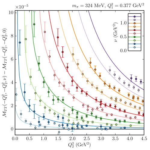
Figure 21: The forward HLbL scattering amplitude ${\cal M}_{\rm TT}$ computed in $N_{f}=2$ lattice QCD and compared to a model for the $\gamma^{*}\gamma^{*}\to{\rm hadrons}$ cross section via the dispersive sum rule (174). Figure from [170].

3.8 Sources of systematic errors in lattice calculations of $a_{\mu}^{\rm hlbl}$

3.8.1 Finite-volume effects

When computing $a_{\mu}^{\rm hlbl}$ using lattice techniques, precisely which formulation is used has a big impact on the systematic effects of the calculation. One important source of systematic error, as in the case of the hadronic vacuum polarisation, are finite-volume effects. Since the photon is massless, an important question is how QED is treated. If it is treated in finite-volume, as in [166, 171], power-law corrections on the result are bound to occur. A quantitative study of these effects was carried out in [171], considering the free-fermion loop contribution to light-by-light scattering in $(g-2)_{\mu}$.

In the strategy laid out in [172, 173], position-space perturbation theory is used to derive an expression for $a_{\mu}^{\rm hlbl}\equiv\hat{F}_{2}(0)$ with QED treated in infinite volume, in order to avoid power-law corrections. Only the QCD four-point function (see Eq. 137) is evaluated in finite volume. Of course this does not necessarily mean that the finite-size effects are then numerically small for the typical volumes used in lattice QCD. A first hint that the finite-size effects might indeed be significant is provided by the calculation of the $\pi^{0}$ pole contribution using the position-space method shown in Fig. 20. For instance, even with a $\pi^{0}$ mass of 600 MeV, an integration up to at least 2 fm is necessary to control the result to within $10\%$. On a torus, the upper bound of integration in the variable $|y|$ is $L/2$ in the least favourable direction, which suggests that $L$ would have to be at least 4 fm, in spite of the large pion mass.

On the other hand, since the pion pole contribution is computable both in finite and in infinite volume, the finite-size effect due to this contribution can be corrected for, provided the pion transition form factor is known. This possibility represents a further motivation for computing the pion transition form factor.

3.8.2 Flavour symmetry and disconnected diagrams in $a_{\mu}^{\rm hlbl}$

The calculation of all Wick-contraction topologies is demanding. In many instances, disconnected diagram contributions have been found to make numerically small contributions to hadronic matrix elements. Quark loops generated by a single vector current have been empirically found to be particularly suppressed; on the other hand, it is well known that the disconnected diagram is responsible for the difference between the pion and the $\eta^{\prime}$ correlator, and is therefore crucial at long distances.

The importance of the disconnected diagrams in the HLbL amplitude has been pointed out in [33, 183], showing that the pion, $\eta$ and $\eta^{\prime}$ pole contributions would have the wrong weight factors if only the connected diagrams were included. This result was re-derived in [179], where it was also shown that if the HLbL amplitude is dominated by the pole-exchange of an iso-vector resonance, isospin symmetry induces relations between different Wick-diagram topologies.

The arguments, based on the large-$N_{c}$ motivated idea that an isolated vector current insertion in a fermion loop gives a suppressed contribution, lead to the conclusion that the (2,2) disconnected class of diagrams in Figure 18 contains all of the contributions from flavour-singlet meson poles, while the mesons in the adjoint representation of the flavour symmetry group contribute with a negative weight factor; the latter is $(-25/9)$ in the SU(2)_flavour case and $(-2)$ in the SU(3)_flavour case. The generic large-$N_{c}$ expectations would further lead to the stronger conclusion that, in each $J^{PC}$ sector, the non-singlet resonances cancel the contribution of the flavour-singlet resonances. One channel, however, where the degeneracy is badly broken is the pseudoscalar sector, since the pion is much lighter than the $\eta^{\prime}$ meson. In particular, at low energies in the two-flavour theory one expects the (2,2) disconnected class of diagrams for a generic HLbL amplitude ${\cal A}$ to be given to a good approximation by

$${\cal A}^{(2+2)}\approx-\frac{25}{9}{\cal A}^{(\pi^{0})}+{\cal A}^{(\eta^{\prime})}\;.$$ (176)

In the case of the forward scattering amplitudes, this prediction was found to be in agreement with the lattice data [45], albeit with a large uncertainty. Similarly, one predicts [45]

$$(a_{\mu}^{\rm hlbl})^{(2,2)}\approx\left\{\begin{array}[]{l@{~~~~}l}-{\displaystyle\frac{25}{9}}(a_{\mu}^{\rm hlbl})^{\pi^{0}}+(a_{\mu}^{\rm hlbl})^{\eta^{\prime}}=-(162\pm 27)\cdot 10^{-11}\hfil~{}~{}~{}~{}&m_{s}=\infty,\phantom{\Big{|}}\\[4.30554pt] -2\left((a_{\mu}^{\rm hlbl})^{\pi^{0}}+(a_{\mu}^{\rm hlbl})^{\eta}\right)+(a_{\mu}^{\rm hlbl})^{\eta^{\prime}}=-(142\pm 19)\cdot 10^{-11}\hfil~{}~{}~{}~{}&m_{s}=m_{ud}.\phantom{\Big{|}}\end{array}\right.,$$ (177)

where one might expect the value in the real world to lie in between these two cases. Taking in addition the result $a_{\mu}^{\rm hlbl}=(102\pm 39)\cdot 10^{-11}$ from a model calculation [167] leads to the following estimate for the fully connected class of diagrams,

$$(a_{\mu}^{\rm hlbl})^{(4)}_{\rm model}\approx\left\{\begin{array}[]{l@{~~~~}l}(264\pm 51)\cdot 10^{-11}\hfil~{}~{}~{}~{}&m_{s}=\infty,\phantom{\Big{|}}\\ (244\pm 46)\cdot 10^{-11}\hfil~{}~{}~{}~{}&m_{s}=m_{ud}.\phantom{\Big{|}}\end{array}\right.$$ (178)

Since the lattice results for $({a_{\mu}^{\rm hlbl}})^{(4)}$ and $({a_{\mu}^{\rm hlbl}})^{(2,2)}$ reviewed in Section 3.5 (see Eqs. (171) and (172)) are significantly smaller in magnitude than these estimates, the authors of [45] conclude that either these lattice results are severely underestimated, which could be due to discretisation and finite-volume effects, or the hadronic model based on resonance exchanges is not viable. Alternatively, the large-$N_{c}$ inspired approximations that are used to estimate (177) and (178) are inadequate. The deviation might also be a combination of the above. New and improved lattice calculations will probably settle the question soon.

4 Concluding remarks

The realisation that the Standard Model does not provide a complete description of nature has sparked a worldwide search for new particles and forces that are collectively referred to as “New Physics” or “Physics beyond the Standard Model” (BSM). Precision observables offer great potential for BSM physics searches, given that new particles have not been discovered at the LHC in the expected region so far. The observed discrepancy of $3.5$ standard deviations between the theoretical and experimental determinations of the muon anomalous magnetic moment constitutes the most intriguing hint for a deviation from the Standard Model, provided that the current estimates and associated uncertainties of hadronic contributions can be trusted. While lattice QCD provides the appropriate framework for the calculation of the hadronic vacuum polarisation and light-by-light scattering contributions from first principles, significant technical challenges must be overcome before lattice results can have a decisive impact on resolving – or confirming – the muon anomaly.

In this review we have outlined the enormous progress that has been achieved in computing both $a_{\mu}^{\rm hvp}$ and $a_{\mu}^{\rm hlbl}$ on the lattice. The precision goals for these two quantities are quite different: while a reliable determination of $a_{\mu}^{\rm hlbl}$ with a total uncertainty of $10-15$% would already have a major impact, lattice calculations of $a_{\mu}^{\rm hvp}$ must reach sub-percent precision, in order to be competitive with the dispersive approach. This requires reliable determinations of finite-volume effects and isospin-breaking corrections, as well as computing the contributions from disconnected diagrams and from the long-distance regime of the vector correlator. The compilation of results for $a_{\mu}^{\rm hvp}$ presented in Section 2.8 shows that the errors of current lattice estimates must be further reduced by a factor $\sim 5$. As calculations of $a_{\mu}^{\rm hvp}$ turn into a flagship project for lattice QCD, with many collaborations attempting to reduce the overall error to a competitive level, there are good prospects that this is achievable within the next few years.

The case of hadronic light-by-light scattering is a lot more complicated, and we have discussed several complementary strategies that are being pursued to determine $a_{\mu}^{\rm hlbl}$ directly or reduce the model dependence considerably. First results from a direct calculation of $a_{\mu}^{\rm hlbl}$ have been published. However, unlike the case of $a_{\mu}^{\rm hvp}$, a complete error budget is not yet available. This task is made more complicated not only because finite-volume effects could be more severe for $a_{\mu}^{\rm hlbl}$, but also since there is a much larger class of disconnected diagrams to be considered. Lattice QCD also provides crucial input for semi-phenomenological approaches, by either replacing experimental input or testing the reliability of hadronic models. For instance, lattice calculations of the transition form factor for $\pi^{0}\to\gamma^{\ast}\gamma^{\ast}$ allow for a reliable determination of the expected dominant contribution to $a_{\mu}^{\rm hlbl}$ from the pion pole. While the results agree with hadronic models, they do not suffer from the arbitrary model-dependent error estimates. Another example is the lattice calculation of a class of forward light-by-light scattering amplitudes, which can be related to phenomenological models via dispersion relations. The combined information from a number of complementary approaches should allow for a much more reliable and largely model-independent determination of $a_{\mu}^{\rm hlbl}$ in the near future.

In order to profit from the new generation of experiments (E989 at Fermilab and E34 at J-PARC) designed to measure $a_{\mu}$ with much enhanced precision, it is clear that theoretical uncertainties must be substantially reduced in the long run. The stated aim of the recently formed “$g-2$ Theory Initiative” is to provide the best theoretical predictions for the hadronic contributions to the muon $g-2$, with lattice QCD being a cornerstone in this endeavour.

Acknowledgements

It is a pleasure to thank the members of the Mainz ($g-2$) project for the fruitful collaboration. In particular, we thank our collaborators A. Gérardin, G. von Hippel, A. Nyffeler, V. Pascalutsa and H. Spiesberger for many stimulating discussions over the past few years. We are grateful to our colleagues within the “$g-2$ Theory Initiative” for interesting discussions and insights. This work was partially supported by DFG via the Collaborative Research Centre “The low-energy frontier of the Standard Model” (SFB 1044), the Rhineland-Palatinate Research Initiative, and by the European Research Council (ERC) under the European Union’s Horizon 2020 research and innovation programme through grant agreement No. 771971-SIMDAMA.

Appendix A Basic concepts of lattice QCD

In this appendix we give a brief and self-contained introduction to lattice QCD. We refrain from providing a general and detailed treatment which can be found in many textbooks [184, 185, 186, 187, 188, 189] and review articles [190]. Instead we shall focus on those aspects of the lattice method that are most relevant for determinations of the hadronic contributions to the muon $g-2$.

A.1 Euclidean path integral and expectation values

Lattice QCD is a rigorous, non-perturbative treatment of the strong interaction that starts from the expression of physical observables in terms of the Euclidean path integral, which is given by

$$Z=\int D[U]D[\overline{\psi},\psi]\,{\rm e}^{-S_{\rm G}[U]-S_{\rm F}[U,\overline{\psi},\psi]},$$ (179)

where $S_{\rm G}$ and $S_{\rm F}$ denote the Euclidean gluon and quark action, respectively, and the integration is performed over all gauge and fermionic fields. After introducing a Euclidean lattice $\Lambda_{\rm E}$ as the finite set of space-time points $x_{\mu}=n_{\mu}a$ that are integer multiples of the lattice spacing $a$ and considering a finite space-time volume of size $L^{3}{\cdot}T$, the path integral is mathematically well defined and finite for suitable gauge invariant discretisations of the gluon and quark action. Thus, the lattice spacing acts as an ultraviolet regulator which preserves gauge invariance at all stages during the evaluation of $Z$.

Gauge fields are represented on the lattice by the link variable $U_{\mu}(x)$ which is an element of the gauge group SU(3). In contrast to QCD formulated in terms of the continuum gauge potential $A_{\mu}(x)$ the integration over the gauge degrees of freedom is performed over the compact group manifold, and thus the typical gauge fixing procedure via the Faddeev-Popov ansatz can be avoided. The simplest discretisation of the gauge action is the Wilson plaquette action [191]

$$S_{\rm G}[U]=\frac{6}{g_{0}^{2}}\sum_{x\in\Lambda_{\rm E}}\sum_{\mu<\nu}\left(1-{\textstyle\frac{1}{3}}{\rm Re\,Tr}\,P_{\mu\nu}(x)\right),$$ (180)

where $P_{\mu\nu}(x)$ denotes the “plaquette”, i.e. the product of link variables around an elementary square in the plane defined by $\mu$ and $\nu$.

A generic expression for the fermionic part of the action is

$$S_{\rm F}[U,\overline{\psi},\psi]=a^{4}\sum_{x\in\Lambda_{\rm E}}\sum_{f=u,d,s,\ldots}\overline{\psi}_{f}(x)\left((D_{\rm lat}[U]+m_{f})\psi_{f}\right)(x),$$ (181)

where $D_{\rm lat}[U]$ denotes the massless discretised Dirac operator, and $m_{f}$ is the mass of quark flavour $f$. Since the quark action is bilinear in the (Grassmannian) fields $\overline{\psi}_{f}$ and $\psi_{f}$ one can perform the integration over the quark fields analytically, which yields

$$Z=\int\prod_{x\in\Lambda_{\rm E}}\prod_{\mu=0}^{3}dU_{\mu}(x)\prod_{f=u,d,s,\ldots}\,{\rm e}^{-S_{\rm G}[U]}\det(D_{\rm lat}[U]+m_{f}).$$ (182)

The path integral now contains a finite number of integrations over the group manifold, while the fermionic part is encoded in the quark determinant. The expectation value of an observable $\Omega$ can then be defined as

$$\left\langle\Omega\right\rangle=\frac{1}{Z}\int\prod_{x\in\Lambda_{\rm E}}\prod_{\mu=0}^{3}dU_{\mu}(x)\;\Omega\prod_{f=u,d,s,\ldots}\,{\rm e}^{-S_{\rm G}[U]}\det(D_{\rm lat}[U]+m_{f}).$$ (183)

The numerical evaluation of $\langle\Omega\rangle$ proceeds by Monte Carlo integration. An ensemble of gauge configurations is generated via importance sampling along a Markov chain, and the factor $W$, defined by

$$W=\prod_{f=u,d,s,\ldots}\det(D_{\rm lat}[U]+m_{f})\,{\rm e}^{-S_{\rm G}[U]},$$ (184)

constitutes the statistical weight of an individual gauge configuration. The most widely used simulation algorithm for QCD with dynamical quarks is the Hybrid Monte Carlo algorithm, originally defined in [192], which has since undergone numerous improvements [193, 194, 195, 196, 197, 198, 199].

Monte Carlo integration is inevitably limited to ensembles containing a finite number of gauge configurations, $N_{\rm cfg}$. Provided that the configurations are sufficiently decorrelated, the gauge average $\overline{\Omega}$ is a good approximation of the expectation value $\langle\Omega\rangle$. Finite statistics also implies a residual uncertainty, so that the result of the integration must be quoted with a statistical error which ideally scales like $1/\sqrt{N_{\rm cfg}}$.

A.2 Lattice actions for QCD

Before performing the stochastic evaluation of $\langle\Omega\rangle$ one must make a concrete choice of lattice action for the gauge field (such as the Wilson plaquette action), as well as the lattice Dirac operator $D_{\rm lat}$. It is important to realise that the discretisation of the QCD action is not unique: Different choices for $S_{\rm G}$ and $S_{\rm F}$ may include any number of irrelevant local operators, provided that they reproduce the Euclidean action in the continuum as the lattice spacing is formally sent to zero. An exhaustive list of common discretisations is given in appendix A.1 of the FLAG report [50].

When choosing a particular discretisation one has to balance computational convenience against conceptual superiority. This is particularly relevant for the choice of quark action and its implications for the treatment of the well-known fermion doubling problem [200, 201, 202] and the closely related issue of chiral symmetry breaking. Here we summarise the general types of fermionic discretisations that are used in current lattice calculations of $a_{\mu}^{\rm hvp}$ and $a_{\mu}^{\rm hlbl}$. For further details we refer to the original articles and appendix A.1 of the FLAG report [50].

Wilson fermions [191] are among the most widely used discretisations of the quark action. The massless Wilson-Dirac operator $D_{\rm w}$ is given by

$$D_{\rm w}={\textstyle\frac{1}{2}}\Big{(}\gamma_{\mu}(\nabla_{\mu}+\nabla_{\mu}^{\ast})-ar\nabla_{\mu}^{\ast}\nabla_{\mu}\Big{)},$$ (185)

where $\nabla_{\mu}$ and $\nabla_{\mu}^{\ast}$ denote the forward and backward discretisations of the covariant derivative, and the Wilson parameter $r$ is typically set to one. The addition of the dimension-5 operator proportional to $r$ implies that $D_{\rm w}$ describes a single fermion species at the expense of explicit chiral symmetry breaking. The consequences of this are two-fold: First, the leading discretisation effects in physical observables are linear in the lattice spacing $a$, and hence the rate of convergence towards the continuum limit is slow. Second, the direct lattice transcription of the electromagnetic current is no longer a conserved quantity. The local vector current in the discretised theory must therefore be renormalised by a multiplicative factor $Z_{\rm V}$ before the Ward identity is satisfied. Still, flavour symmetry remains intact in this formulation. Furthermore, a conserved vector current can be derived from the Wilson action via the usual Noether procedure. More details are provided in A.3.

The leading discretisation effects of ${\rm{O}}(a)$ can be removed via the Symanzik improvement programme [203, 204], which is achieved by adding a suitable counterterm to the Wilson-Dirac operator. This results in the so-called Sheikholeslami-Wohlert or “Clover” action [205], i.e.

$$D_{\rm sw}=D_{\rm w}+\frac{ia}{4}c_{\rm{sw}}\sigma_{\mu\nu}\widehat{F}_{\mu\nu},$$ (186)

where $\widehat{F}$ is a lattice transcription of the gluon field strength tensor, $\sigma_{\mu\nu}=\frac{i}{2}[\gamma_{\mu},\gamma_{\nu}]$ and the coefficient $c_{\rm{sw}}$ must be tuned appropriately to achieve the complete cancellation of ${\rm{O}}(a)$ lattice artefacts. The currents and other local composite operators must be improved as well by adding appropriate counterterms [206, 207, 208].

Twisted mass Wilson fermions: The removal of the leading cutoff effects can also be accomplished by adding a chirally twisted mass term to the Wilson action [209]. In two-flavour QCD the corresponding operator describing “twisted mass QCD” (tmQCD) is

$$D_{\rm tm}^{(m)}=D_{\rm w}+m_{f}+i\mu_{f}\gamma_{5}\tau^{3},$$ (187)

where $\mu_{f}$ is the twisted mass parameter of flavour $f$, and the superscript “$(m)$” on the operator indicates that the massive operator is considered. The ratio $\mu_{\rm R}/m_{\rm R}$ of the renormalised twisted and standard quark masses defines the twist angle, i.e.

$$\tan\alpha_{\rm R}=\frac{\mu_{\rm R}}{m_{\rm R}}.$$ (188)

In Ref. [210] it was shown that the leading cutoff effects of ${\rm{O}}(a)$ are cancelled without the addition of the Sheikholeslami-Wohlert term, by tuning the bare parameters such that $\alpha_{\rm R}=\pi/2$ (“maximal twist”).

The presence of the twisted mass parameter introduces a tunable infrared scale. This is helpful for reducing the numerical effort in the simulation of the theory in the regime of small quark masses, where the occurrence of small eigenvalues of the Dirac operator may lead to a small acceptance rate in the HMC algorithm. However, one finds that isospin symmetry is broken in twisted mass QCD.

Staggered fermions [211, 212] leave a subgroup of chiral symmetry unbroken but achieve only a partial lifting of the 16-fold degeneracy that is encountered if $r$ is set to zero in Eq. (185), resulting in four fermionic doubler states, which are commonly referred to as “tastes”. To remove this residual degeneracy one takes fractional powers of the quark determinant, a procedure known as “rooting”. Since the taste symmetry is broken by the interaction with gluons, the rooting procedure produces unitarity violations. The validity of the rooting procedure has been contested in Refs. [213, 214]. On the other hand, arguments based on a renormalisation-group approach [215, 216] suggest that rooted staggered quarks reproduce the correct, unitary theory in the continuum limit.

The staggered formulation is numerically inexpensive compared to Wilson-type fermions, since the application of the staggered Dirac operator requires fewer floating-point operations. The leading lattice artefacts are of order $a^{2}$ without the necessity for twisting or the addition of counterterms. Furthermore, staggered fermions do not suffer from accidentally small eigenvalues that slow down the simulation. These practical advantages must be balanced against the rooting issue. Violations of the taste symmetry and the overall influence of cutoff effects can be reduced with the help of the Symanzik improvement programme [217]. The resulting variants of the staggered action are referred to as the “Asqtad” [218] and “HISQ” [219] actions.

Ginsparg Wilson fermions [220, 221, 222, 223, 224] preserve chiral symmetry whilst removing all doublers from the fermion spectrum. The associated Dirac operator $D$ satisfies

$$\gamma_{5}D+D\gamma_{5}=aD\gamma_{5}D,$$ (189)

which is known as the Ginsparg-Wilson relation [220]. It represents a modification of the usual requirement that a chirally invariant Dirac operator in the continuum must anticommute with $\gamma_{5}$. Explicit constructions of an operator that satisfies Eq. (189) include the “domain wall” formulation [225] in which a $5^{\rm th}$ dimension of length $N_{5}$ is introduced while the fermions are coupled to a mass defect, i.e. a negative mass term. One then finds that modes of opposite chirality are trapped at the 4-dimensional boundaries. For any finite values of $N_{5}$, however, the decoupling of chiral modes is not exact, leading to residual though exponentially suppressed chiral symmetry breaking. Domain wall fermions have been employed by the RBC/UKQCD Collaboration in their calculations of $a_{\mu}^{\rm hvp}$ and $a_{\mu}^{\rm hlbl}$. In addition to the domain wall construction of Ginsparg-Wilson fermions, there are other realisations of operators which satisfy Eq. (189). These include the “overlap” or “Neuberger-Dirac” operator [221, 222], as well as the truncated fixed point [226] and “chirally improved” [227] actions. None of these have so far been applied in determinations of the hadronic contributions to $(g-2)_{\mu}$.

While Ginsparg-Wilson fermions respect all flavour and chiral symmetries and reproduce the correct fermion spectrum, they are numerically much more costly that Wilson or staggered fermions. This is due to the fact that the operator is defined on a 5-dimensional lattice in the case of domain wall fermions. If Ginsparg-Wilson fermions are instead realised via the overlap operator, one is faced with the problem of evaluating the sign function of a large sparse matrix.

A.3 Vector currents and renormalisation

Both the hadronic vacuum polarisation and light-by-light scattering contributions to $a_{\mu}$ are expressed in terms of the electromagnetic current

$$J_{\mu}(x)=\sum_{f=u,d,s,\ldots}{\cal{Q}}_{f}\overline{\psi}_{f}(x)\gamma_{\mu}\psi_{f}(x),$$ (190)

where ${\cal{Q}}_{f}$ denotes the electric charge of quark flavour $f$. In the continuum, the Ward identities ensure that the current is conserved, i.e.

$$\partial_{\mu}J_{\mu}(x)=0.$$ (191)

However, if the theory is regularised by introducing any of the discretisations discussed above, one finds that the counterpart of $J_{\mu}(x)$ is not the symmetry current which can be derived using Noether’s theorem. The introduction of a lattice cutoff modifies the theory in the ultraviolet, and these short-distance effects must, in general, be absorbed into a renormalisation factor. Below we describe several variants of vector currents that are used in current calculations of $a_{\mu}^{\rm hvp}$ and $a_{\mu}^{\rm hlbl}$.

Omitting the electric charge factors one defines the local vector current in the lattice regularised theory for quark flavour $f$ by

$$V_{\mu}^{f}(x)=\overline{\psi}_{f}(x)\gamma_{\mu}\psi_{f}(x).$$ (192)

In general, $V_{\mu}^{f}(x)$ is renormalised multiplicatively by a factor $Z_{\rm V}$ which depends on the bare gauge coupling $g_{0}$. While the renormalisation factor $Z_{\rm V}$ can be computed in lattice perturbation theory, it is well known that the perturbative expansion in powers of the bare coupling $g_{0}^{2}$ has poor convergence properties [228]. Several methods have been developed that allow for the non-perturbative determination of $Z_{\rm V}$ and can also be applied to the renormalisation of many other local operators. In a first step one defines a scheme that allows for imposing a non-perturbative renormalisation condition for the operator under consideration. In the second step this condition is evaluated in a numerical simulation. The most widely used schemes are based on the Schrödinger functional [229, 230, 231, 208] and the regularisation-independent momentum subtraction (RI-MOM) scheme [232] and its variants [233]. A simple renormalisation condition for the vector current, which can also be evaluated with good statistical precision, demands that the forward matrix element of the current between pseudoscalar mesons be equal to one, which yields (ignoring quark-mass dependent O($a$) effects)

$$\frac{1}{Z_{\rm V}}=\frac{\left\langle P,\boldsymbol{q}\left|V_{0}^{f}\right|P,\boldsymbol{q}\right\rangle}{\left\langle P,\boldsymbol{q}|P,\boldsymbol{q}\right\rangle},$$ (193)

where $|P,\boldsymbol{q}\rangle$ denotes a pseudoscalar meson state consisting of quarks with flavour $f$ and momentum $\boldsymbol{q}$.

Below we discuss variants of the vector current for different discretisations. If the fermionic part of the QCD action is discretised using the Wilson quark action, the leading discretisation effects of ${\rm{O}}(a)$ can be cancelled by adding the Sheikholeslami-Wohlert term to the action. While this ensures that spectral quantities such as hadron masses approach the continuum limit with a rate proportional to $a^{2}$, this is not true for operator matrix elements involving the current. In isospin-symmetric QCD, the general form of the renormalised isovector vector current, which is consistent with ${\rm{O}}(a)$ improvement reads [206, 208, 234]

$$(V_{\mu}^{u}(x)-V_{\mu}^{d}(x))_{\rm R} = Z_{\rm V}(\tilde{g}_{0})(1+\bar{b}_{\rm V}\;a{\rm Tr}(M)+b_{\rm V}\;am_{ud})\times$$

$$\times\left\{V_{\mu}^{u}(x)-V_{\mu}^{d}(x)+ac_{\rm V}\partial_{\nu}(T_{\mu\nu}^{u}(x)-T_{\mu\nu}^{d}(x))\right\},$$

where $b_{\rm V},\,\bar{b}_{\rm V},\,c_{\rm V}$ are improvement coefficients that depend on the gauge coupling. In this expression, $\tilde{g}_{0}$ denotes the modified gauge coupling consistent with O($a$) improvement [206], $M$ is the bare subtracted quark-mass matrix, with elements $M_{11}=M_{22}=m_{ud}$ corresponding to the light flavours $u,d$, and

$$T_{\mu\nu}^{f}(x)=i\overline{\psi}_{f}(x)\sigma_{\mu\nu}\psi_{f}(x)$$ (195)

is the tensor current. While $Z_{\rm V}$ and the improvement coefficient $b_{\rm V}$ have been calculated in perturbation theory [235], a non-perturbative determination is desirable. The coefficient $c_{\rm V}$ has been addressed in [236, 237, 238, 239]; the coefficients $b_{\rm V}$ and $\bar{b}_{\rm V}$ were computed by different methods in [240, 241]. Recently, a high-accuracy determination of the renormalisation factors of the vector and axial-vector currents in the massless theory was achieved [242] by using the chirally rotated Schrödinger functional framework [243, 244]. The presence of the terms proportional to $b_{\rm V}$ and $\bar{b}_{\rm V}$ implies that the renormalisation factor contains a mass-dependent piece. The improvement of the isoscalar part of the electromagnetic current involves an additional improvement coefficient $f_{\rm V}$, which contributes to an O($a$) mass-dependent counterterm proportional to the flavour-singlet current [234].

As an alternative, one can use the vector current derived from the Wilson action via Noether’s theorem, i.e.

$$\hat{V}_{\mu}^{f}(x)=\frac{1}{2}\left\{\overline{\psi}_{f}(x+a\hat{\mu})(1+\gamma_{\mu})U_{\mu}(x)^{\dagger}\psi_{f}(x)-\overline{\psi}_{f}(x)(1-\gamma_{\mu})U_{\mu}(x)\psi_{f}(x+a\hat{\mu})\right\},$$ (196)

which is also referred to as the “point-split” vector current, as it contains fields located at neighbouring lattice sites. Since $\hat{V}_{\mu}^{f}$ is conserved by construction, the multiplicative renormalisation factor is trivial, $Z_{\rm\hat{V}}=1$. As it stands, the point-split current in Eq. (196) is, however, not improved. An ${\rm{O}}(a)$ improved, renormalised version of $\hat{V}_{\mu}(x)$ requires an additive counterterm given by the divergence of the tensor current, analogously to the term present in Eq. (A.3). Non-perturbative determinations of the improvement coefficient $c_{\rm V}$ have been described in [236, 238, 239].

Domain wall fermions: The lattice Dirac operator describing domain wall fermions reads

$$D_{\rm dwf}=\left(D_{\rm w}-M\right)_{xy}\delta_{st}+\delta_{xy}D_{st}^{(5)},$$ (197)

where $s,t$ label coordinates along the $5^{\rm th}$ dimension of length $N_{5}$, $D_{\rm st}^{(5)}$ is the corresponding coupling term, and the parameter $M$ denotes the domain wall height. Quark fields that are defined on the 4-dimensional subspace are obtained through the projection [225]

$$q(x)=P_{+}\psi(x,N_{5}-1)+P_{-}\psi(x,0),\quad P_{\pm}={\textstyle\frac{1}{2}}\left(1\pm\gamma_{5}\right),$$ (198)

where the fermion field $\psi(x,s)$ is defined on the full 5-dimensional manifold. The local vector current is defined as

$$V_{\mu}(x)=\overline{q}(x)\gamma_{\mu}q(x),$$ (199)

while the expression for the conserved current is quite similar to Eq. (196), i.e.

$$\hat{V}_{\mu}(x)=\frac{1}{2}\sum_{s=1}^{N_{5}}\left\{\overline{\psi}(x+a\hat{\mu},s)(1+\gamma_{\mu})U_{\mu}(x)^{\dagger}\psi(x,s)\right.\left.-\;\overline{\psi}(x,s)(1-\gamma_{\mu})U_{\mu}(x)\psi(x+a\hat{\mu},s)\right\}.$$ (200)

Since the decoupling of chiral modes is only exact for $N_{5}\to\infty$, the renormalisation factor of $\hat{V}_{\mu}(x)$ differs from unity by terms proportional to the residual additive renormalisation of the quark mass, i.e. $Z_{\rm\hat{V}}=1+{\rm{O}}(am_{\rm res})$.

A.4 Vector correlator and polarisation tensor on the lattice

Using for simplicity the definitions of the conserved vector currents in the previous section, one obtains the expression for the vacuum polarisation tensor of Eq. (9) on a space-time lattice as

$$\Pi_{\mu\nu}({Q})=a\,\delta_{\mu\nu}\,\sum_{f}{\cal{Q}}_{f}^{2}\,\langle T^{f}_{\mu}(0)\rangle+a^{4}\sum_{f,f^{\prime}}\,{\cal{Q}}_{f}{\cal{Q}}_{f^{\prime}}\sum_{x}\,{\rm e}^{iQ(x+\frac{a}{2}(\hat{\mu}-\hat{\nu}))}\,\left\langle\hat{V}_{\mu}^{f}(x)\hat{V}_{\nu}^{f^{\prime}}(0)\right\rangle,$$ (201)

where ${\cal{Q}}_{f},{\cal{Q}}_{f^{\prime}}$ denote the electric charges of quark flavours $f$ and $f^{\prime}$. The role of the tadpole terms $\langle T^{f}_{\mu}(0)\rangle$ is to remove a quadratic divergence [52], but we also note that this term drops out in the subtraction performed in Eq. (203) below. The polarisation tensor given in Eq. (201) is transverse in the following sense:

$$\sum_{\mu=0}^{3}\hat{Q}_{\mu}\;\Pi_{\mu\nu}({Q})=\sum_{\nu=0}^{3}\hat{Q}_{\nu}\;\Pi_{\mu\nu}({Q})=0,$$ (202)

where $\hat{Q}=\frac{2}{a}\sin\left(aQ_{\mu}/2\right)$ is the lattice momentum. Note that on a finite space-time lattice, the momentum variable $Q_{\mu}$ assumes integer multiples of $2\pi/L_{\mu}$, where $L_{\mu}$ is the length in direction $\mu$.

It has been noted in [94, 145] (see also [146, 171]) that the vacuum polarisation tensor does not vanish at $Q=0$ in finite volume, $\Pi_{\mu\nu}(0)\neq 0$. In order to reduce finite-volume effects and to suppress the short-distance region, it is then advantageous to subtract the contribution $\Pi_{\mu\nu}(0)$, which is easily accomplished via a simple modification of the phase factor in Eq. (201), i.e.

$$\Pi_{\mu\nu}({Q})-\Pi_{\mu\nu}({0})=a^{4}\sum_{f,f^{\prime}}{\cal{Q}}_{f}{\cal{Q}}_{f^{\prime}}\sum_{x}\,\left({\rm{e}}^{iQ(x+\frac{a}{2}(\hat{\mu}-\hat{\nu}))}-1\right)\left\langle\hat{V}_{\mu}^{f}(x)\hat{V}_{\nu}^{f^{\prime}}(0)\right\rangle.$$ (203)

The spatially summed vector correlator, $G(x_{0})$, is the central quantity for the determination of $a_{\mu}^{\rm hvp}$ using the time-momentum representation (see Eq. (20)). On the lattice the corresponding expression reads

$$G(x_{0})\delta_{kl}=-a^{3}\sum_{f,f^{\prime}}{\cal{Q}}_{f}{\cal{Q}}_{f^{\prime}}\sum_{\boldsymbol{x}}\left\langle\hat{V}_{k}^{f}(x)\hat{V}_{l}^{f^{\prime}}(0)\right\rangle.$$ (204)

In the case of Wilson fermions, the improvement term proportional to the divergence of the tensor current must implicitly be included in the vector currents appearing in Eq. (204), if full O($a$) improvement is to be achieved. The sum $\sum_{f,f^{\prime}}\ldots$ in equations (201), (203) and (204) runs over all quark flavours included in the electromagnetic currents. However, one is often interested in the contributions to $a_{\mu}^{\rm hvp}$ from individual quark flavours. Noting that the dominant contributions arise from quark-connected diagrams, one defines

$$\Pi_{\mu\nu}^{f}({Q})={\cal{Q}}_{f}^{2}\,\Big{(}a\,\delta_{\mu\nu}\,\langle T^{f}_{\mu}(0)\rangle+a^{4}\sum_{x}\,{\rm{e}}^{iQ(x+\frac{a}{2}(\hat{\mu}-\hat{\nu}))}\,\left\langle\hat{V}_{\mu}^{f}(x)\hat{V}_{\nu}^{f}(0)\right\rangle\Big{)},$$ (205)

$$G^{f}(x_{0})=-\frac{a^{3}}{3}{\cal{Q}}_{f}^{2}\sum_{\boldsymbol{x}}\left\langle\hat{V}_{k}^{f}(x)\hat{V}_{k}^{f}(0)\right\rangle,\quad f=(ud),s,c,\ldots$$ (206)

In the above expressions it is understood that the expectation value is restricted to quark-connected diagrams only. We have assumed that the up and down quarks are mass-degenerate, $m_{u}=m_{d}$ while ${\cal{Q}}_{ud}^{2}=5/9$. By performing the tensor decomposition according to Eq. (11) one obtains $\Pi^{f}(Q^{2})$, i.e. the (connected) contribution of quark flavour $f$ to the vacuum polarisation function. The corresponding fraction of the anomalous magnetic moment, $(a_{\mu}^{\rm hvp})^{f}$, is obtained by inserting $\Pi^{f}(Q^{2})$ and $G^{f}(x_{0})$ into equations (13) and (26), respectively.

A.5 Systematic effects

Below we give an overview of the main systematic effects that are common to all lattice calculations.

Discretisation errors: Lattice estimates of renormalised, dimensionless quantities differ from their continuum counterparts by terms proportional to $a^{p}$, where $a$ denotes the lattice spacing, and the positive integer $p$ depends on the details of the discretisation. In order to obtain the result in the continuum limit, an extrapolation of data computed at several values of the lattice spacing must be performed. Obviously, the convergence to the continuum limit is faster for large values of $p$. While $p=1$ for unimproved Wilson fermions, one finds $p=2$ for most other fermionic discretisations, including staggered, domain wall and twisted-mass Wilson fermions. The Symanzik improvement programme, when applied to Wilson fermions, also yields $p=2$. Typical values of the lattice spacing in current simulations are of order $0.1\,{\rm{fm}}$ and smaller.

Quark mass dependence: Quark masses are “external” parameters of QCD that cannot determined by the theory itself. In lattice simulations the physical values of the quark masses are a priori unknown and must be fixed by comparing lattice results to experiment. To this end one computes observables at several different values of the bare quark mass and determines the result corresponding to the physical situation by an inter- or extrapolation in the quark mass. The ansatz used to fit the quark mass dependence is often motivated by chiral effective theory.

Before the mid-2000s, lattice simulations with dynamical quarks had been restricted to unphysically large values of the up and down-quark masses, since the numerical effort for producing statistically decorrelated configurations showed a strong growth as the chiral regime was approached. Lattice results were therefore subject to a potentially large systematic uncertainty arising from chiral extrapolations to the physical point. Thanks to a number of algorithmic improvements [193, 194, 195, 196, 197, 198, 199] and increasing numerical resources, simulations at or very near the physical pion mass are now carried out on a routine basis, so that the uncertainty associated with the quark mass dependence of observables can be significantly reduced.

Finite volume effects: Results computed in lattice simulations are usually affected by the finite extent of the spatial and temporal dimensions of the lattice. It can be shown, however, that finite-volume effects in stable hadron masses, decay constants and spacelike form factors are exponentially suppressed, provided that the spatial size in unit of the mass of the lightest bound state, the pion, is sufficiently large. Finite-volume effects thus contain the universal factor $\exp\{-(m_{\pi}L)\}$, and one finds empirically that for many quantities such as hadron masses and decay constants they are negligible provided that

$$m_{\pi}L\gtrsim 4.$$ (207)

Obviously, this criterion is not universally applicable and must be verified on a case-by-case basis.

Finite-volume effects are not just a nuisance in lattice calculations but offer a method to gain information on hadronic systems. The Lüscher method [245, 246, 97, 98] is a powerful formalism for the characterisation of resonances in lattice QCD, by providing an exact relation between scattering phase shifts and the energy levels of multi-particle states in a finite volume. As we will see later in this review, this is highly relevant for the determination of the hadronic vacuum polarisation contribution.

While it is very costly to perform simulations for the same set of parameters on different volumes to check whether the results show a significant dependence on the extent of the lattice, one can also employ effective theories such as Chiral Perturbation Theory to estimate finite-volume effects [247, 248, 249, 250].

Critical slowing down: The most widely used simulation algorithm for dynamical fermions, the Hybrid Monte Carlo (HMC) algorithm becomes rapidly inefficient at producing decorrelated gauge configurations as the lattice spacing is reduced to $a\lesssim 0.05\,{\rm{fm}}$. This is commonly referred to as “critical slowing down”. Gauge configurations can be classified in terms of their topological properties, characterised by the winding number or topological charge. Critical slowing down manifests itself in the observed inability of the HMC algorithm to tunnel between different sectors of topological charge, which results in extremely long autocorrelation times [251]. As a result the statistical errors that are assigned to the results may not be reliable. A number of proposals have been suggested to alleviate the problem of “topology freezing” and the associated autocorrelation times, including the use of open boundary conditions [252] or multi-scale Monte Carlo equilibration [253].

References

- [1] G. W. Bennett, et al., Final Report of the Muon E821 Anomalous Magnetic Moment Measurement at BNL, Phys. Rev. D73 (2006) 072003. arXiv:hep-ex/0602035, doi:10.1103/PhysRevD.73.072003.
- [2] D. Hanneke, S. F. Hoogerheide, G. Gabrielse, Cavity Control of a Single-Electron Quantum Cyclotron: Measuring the Electron Magnetic Moment, Phys. Rev. A83 (2011) 052122. arXiv:1009.4831, doi:10.1103/PhysRevA.83.052122.
- [3] R. Parker, C. Yu, W. Zhong, B. Estey, H. Mueller, Measurement of the fine-structure constant as a test of the Standard Model, Science 360 (2018) 191–195. doi:10.1126/science.aap7706.
- [4] F. Jegerlehner, A. Nyffeler, The Muon , Phys. Rept. 477 (2009) 1–110. arXiv:0902.3360, doi:10.1016/j.physrep.2009.04.003.
- [5] T. Blum, A. Denig, I. Logashenko, E. de Rafael, B. Lee Roberts, et al., The Muon () Theory Value: Present and FuturearXiv:1311.2198.
- [6] F. Jegerlehner, The Anomalous Magnetic Moment of the Muon, Springer Tracts Mod. Phys. 274 (2017) pp.1–693. doi:10.1007/978-3-319-63577-4.
- [7] T. Aoyama, M. Hayakawa, T. Kinoshita, M. Nio, Complete Tenth-Order QED Contribution to the Muon g-2, Phys. Rev. Lett. 109 (2012) 111808. arXiv:1205.5370, doi:10.1103/PhysRevLett.109.111808.
- [8] A. Czarnecki, W. J. Marciano, A. Vainshtein, Refinements in electroweak contributions to the muon anomalous magnetic moment, Phys. Rev. D67 (2003) 073006, [Erratum: Phys. Rev.D73,119901(2006)]. arXiv:hep-ph/0212229, doi:10.1103/PhysRevD.67.073006,10.1103/PhysRevD.73.119901.
- [9] C. Gnendiger, D. Stöckinger, H. Stöckinger-Kim, The electroweak contributions to after the Higgs boson mass measurement, Phys. Rev. D88 (2013) 053005. arXiv:1306.5546, doi:10.1103/PhysRevD.88.053005.
- [10] M. Davier, A. Hoecker, B. Malaescu, Z. Zhang, Reevaluation of the hadronic vacuum polarisation contributions to the Standard Model predictions of the muon and using newest hadronic cross-section data, Eur. Phys. J. C77 (12) (2017) 827. arXiv:1706.09436, doi:10.1140/epjc/s10052-017-5161-6.
- [11] A. Kurz, T. Liu, P. Marquard, M. Steinhauser, Hadronic contribution to the muon anomalous magnetic moment to next-to-next-to-leading order, Phys. Lett. B734 (2014) 144–147. arXiv:1403.6400, doi:10.1016/j.physletb.2014.05.043.
- [12] J. Prades, E. de Rafael, A. Vainshtein, The Hadronic Light-by-Light Scattering Contribution to the Muon and Electron Anomalous Magnetic Moments, Adv. Ser. Direct. High Energy Phys. 20 (2009) 303–317. arXiv:0901.0306, doi:10.1142/9789814271844\_0009.
- [13] S. J. Brodsky, E. De Rafael, Suggested boson - lepton pair couplings and the anomalous magnetic moment of the muon, Phys. Rev. 168 (1968) 1620–1622. doi:10.1103/PhysRev.168.1620.
- [14] M. Davier, A. Höcker, B. Malaescu, Z. Zhang, Reevaluation of the Hadronic Contributions to the Muon and to , Eur. Phys. J. C71 (2011) 1515. arXiv:1010.4180, doi:10.1140/epjc/s10052-010-1515-z.
- [15] F. Jegerlehner, R. Szafron, mixing in the neutral channel pion form factor and its role in comparing with spectral functions, Eur. Phys. J. C71 (2011) 1632. arXiv:1101.2872, doi:10.1140/epjc/s10052-011-1632-3.
- [16] K. Hagiwara, R. Liao, A. D. Martin, D. Nomura, T. Teubner, and re-evaluated using new precise data, J.Phys. G38 (2011) 085003. arXiv:1105.3149, doi:10.1088/0954-3899/38/8/085003.
- [17] F. Jegerlehner, Muon theory: The hadronic part, EPJ Web Conf. 166 (2018) 00022. arXiv:1705.00263, doi:10.1051/epjconf/201816600022.
- [18] A. Keshavarzi, D. Nomura, T. Teubner, The muon and : a new data-based analysis, Phys. Rev. D97 (11) (2018) 114025. arXiv:1802.02995, doi:10.1103/PhysRevD.97.114025.
- [19] F. Ambrosino, et al., Measurement of and the dipion contribution to the muon anomaly with the KLOE detector, Phys. Lett. B670 (2009) 285–291. arXiv:0809.3950, doi:10.1016/j.physletb.2008.10.060.
- [20] F. Ambrosino, et al., Measurement of from threshold to 0.85 GeV2 using Initial State Radiation with the KLOE detector, Phys. Lett. B700 (2011) 102–110. arXiv:1006.5313, doi:10.1016/j.physletb.2011.04.055.
- [21] D. Babusci, et al., Precision measurement of and determination of the contribution to the muon anomaly with the KLOE detector, Phys. Lett. B720 (2013) 336–343. arXiv:1212.4524, doi:10.1016/j.physletb.2013.02.029.
- [22] J. P. Lees, et al., Precise Measurement of the Cross Section with the Initial-State Radiation Method at BABAR, Phys. Rev. D86 (2012) 032013. arXiv:1205.2228, doi:10.1103/PhysRevD.86.032013.
- [23] M. Ablikim, et al., Measurement of the cross section between 600 and 900 MeV using initial state radiation, Phys. Lett. B753 (2016) 629–638. arXiv:1507.08188, doi:10.1016/j.physletb.2015.11.043.
- [24] R. Alemany, M. Davier, A. Höcker, Improved determination of the hadronic contribution to the muon and to using new data from hadronic tau decays, Eur. Phys. J. C2 (1998) 123–135. arXiv:hep-ph/9703220, doi:10.1007/s100520050127.
- [25] M. Hayakawa, T. Kinoshita, A. I. Sanda, Hadronic light by light scattering contribution to muon g-2, Phys. Rev. D54 (1996) 3137–3153. arXiv:hep-ph/9601310, doi:10.1103/PhysRevD.54.3137.
- [26] M. Hayakawa, T. Kinoshita, Pseudoscalar pole terms in the hadronic light by light scattering contribution to muon g - 2, Phys. Rev. D57 (1998) 465–477, [Erratum: Phys. Rev.D66,019902(2002)]. arXiv:hep-ph/9708227, doi:10.1103/PhysRevD.57.465,10.1103/PhysRevD.66.019902.
- [27] J. Bijnens, E. Pallante, J. Prades, Hadronic light by light contributions to the muon g-2 in the large N(c) limit, Phys. Rev. Lett. 75 (1995) 1447–1450, [Erratum: Phys. Rev. Lett.75,3781(1995)]. arXiv:hep-ph/9505251, doi:10.1103/PhysRevLett.75.1447.
- [28] J. Bijnens, E. Pallante, J. Prades, Analysis of the hadronic light by light contributions to the muon g-2, Nucl. Phys. B474 (1996) 379–420. arXiv:hep-ph/9511388, doi:10.1016/0550-3213(96)00288-X.
- [29] J. Bijnens, E. Pallante, J. Prades, Comment on the pion pole part of the light by light contribution to the muon g-2, Nucl. Phys. B626 (2002) 410–411. arXiv:hep-ph/0112255, doi:10.1016/S0550-3213(02)00074-3.
- [30] M. Knecht, A. Nyffeler, Hadronic light by light corrections to the muon : The Pion pole contribution, Phys. Rev. D65 (2002) 073034. arXiv:hep-ph/0111058, doi:10.1103/PhysRevD.65.073034.
- [31] K. Melnikov, A. Vainshtein, Hadronic light-by-light scattering contribution to the muon anomalous magnetic moment revisited, Phys. Rev. D70 (2004) 113006. arXiv:hep-ph/0312226, doi:10.1103/PhysRevD.70.113006.
- [32] A. Nyffeler, Hadronic light-by-light scattering in the muon g-2: A New short-distance constraint on pion-exchange, Phys. Rev. D79 (2009) 073012. arXiv:0901.1172, doi:10.1103/PhysRevD.79.073012.
- [33] J. Bijnens, Hadronic light-by-light contribution to : extended Nambu-Jona-Lasinio, chiral quark models and chiral Lagrangians, in: Proceedings, Workshop on Flavour changing and conserving processes 2015 (FCCP2015): Anacapri, Capri Island, Italy, September 10-12, 2015, Vol. 118, 2016, p. 01002. arXiv:1510.05796, doi:10.1051/epjconf/201611801002.
- [34] G. Colangelo, M. Hoferichter, M. Procura, P. Stoffer, Dispersive approach to hadronic light-by-light scattering, JHEP 09 (2014) 091. arXiv:1402.7081, doi:10.1007/JHEP09(2014)091.
- [35] G. Colangelo, M. Hoferichter, B. Kubis, M. Procura, P. Stoffer, Towards a data-driven analysis of hadronic light-by-light scattering, Phys. Lett. B738 (2014) 6–12. arXiv:1408.2517, doi:10.1016/j.physletb.2014.09.021.
- [36] G. Colangelo, M. Hoferichter, M. Procura, P. Stoffer, Dispersion relation for hadronic light-by-light scattering: theoretical foundations, JHEP 09 (2015) 074. arXiv:1506.01386, doi:10.1007/JHEP09(2015)074.
- [37] G. Colangelo, M. Hoferichter, M. Procura, P. Stoffer, Rescattering effects in the hadronic-light-by-light contribution to the anomalous magnetic moment of the muon, Phys. Rev. Lett. 118 (23) (2017) 232001. arXiv:1701.06554, doi:10.1103/PhysRevLett.118.232001.
- [38] G. Colangelo, M. Hoferichter, M. Procura, P. Stoffer, Dispersion relation for hadronic light-by-light scattering: two-pion contributions, JHEP 04 (2017) 161. arXiv:1702.07347, doi:10.1007/JHEP04(2017)161.
- [39] V. Pascalutsa, M. Vanderhaeghen, Sum rules for light-by-light scattering, Phys. Rev. Lett. 105 (2010) 201603. arXiv:1008.1088, doi:10.1103/PhysRevLett.105.201603.
- [40] V. Pascalutsa, V. Pauk, M. Vanderhaeghen, Light-by-light scattering sum rules constraining meson transition form factors, Phys. Rev. D85 (2012) 116001. arXiv:1204.0740, doi:10.1103/PhysRevD.85.116001.
- [41] V. Pauk, M. Vanderhaeghen, Two-loop massive scalar three-point function in a dispersive approacharXiv:1403.7503.
- [42] V. Pauk, M. Vanderhaeghen, Anomalous magnetic moment of the muon in a dispersive approach, Phys. Rev. D90 (11) (2014) 113012. arXiv:1409.0819, doi:10.1103/PhysRevD.90.113012.
- [43] I. Danilkin, M. Vanderhaeghen, Light-by-light scattering sum rules in light of new data, Phys. Rev. D95 (1) (2017) 014019. arXiv:1611.04646, doi:10.1103/PhysRevD.95.014019.
- [44] A. Nyffeler, Precision of a data-driven estimate of hadronic light-by-light scattering in the muon : Pseudoscalar-pole contribution, Phys. Rev. D94 (5) (2016) 053006. arXiv:1602.03398, doi:10.1103/PhysRevD.94.053006.
- [45] A. Gérardin, H. B. Meyer, A. Nyffeler, Lattice calculation of the pion transition form factor , Phys. Rev. D94 (7) (2016) 074507. arXiv:1607.08174, doi:10.1103/PhysRevD.94.074507.
- [46] M. Hoferichter, B.-L. Hoid, B. Kubis, S. Leupold, S. P. Schneider, Pion-pole contribution to hadronic light-by-light scattering in the anomalous magnetic moment of the muon, Phys. Rev. Lett. 121 (2018) 112002. arXiv:1805.01471, doi:10.1103/PhysRevLett.121.112002.
- [47] J. Kaspar, Status of the Fermilab experiment, Nucl. Part. Phys. Proc. 260 (2015) 243–246. arXiv:1504.01201, doi:10.1016/j.nuclphysbps.2015.02.051.
- [48] M. Fertl, Next generation muon experiment at FNAL, Hyperfine Interact. 237 (1) (2016) 94. arXiv:1610.07017, doi:10.1007/s10751-016-1304-7.
- [49] M. Otani, Design of the J-PARC MUSE H-line for the Muon g-2/EDM Experiment at J-PARC (E34), JPS Conf. Proc. 8 (2015) 025010. doi:10.7566/JPSCP.8.025010.
- [50] S. Aoki, et al., Review of lattice results concerning low-energy particle physics, Eur. Phys. J. C77 (2) (2017) 112. arXiv:1607.00299, doi:10.1140/epjc/s10052-016-4509-7.
- [51] T. Blum, Lattice calculation of the lowest order hadronic contribution to the muon anomalous magnetic moment, Phys. Rev. Lett. 91 (2003) 052001. arXiv:hep-lat/0212018, doi:10.1103/PhysRevLett.91.052001.
- [52] M. Göckeler, et al., Vacuum polarization and hadronic contribution to muon from lattice QCD, Nucl. Phys. B688 (2004) 135–164. arXiv:hep-lat/0312032, doi:10.1016/j.nuclphysb.2004.03.026.
- [53] C. Aubin, T. Blum, Calculating the hadronic vacuum polarization and leading hadronic contribution to the muon anomalous magnetic moment with improved staggered quarks, Phys. Rev. D75 (2007) 114502. arXiv:hep-lat/0608011, doi:10.1103/PhysRevD.75.114502.
- [54] X. Feng, K. Jansen, M. Petschlies, D. B. Renner, Two-flavor QCD correction to lepton magnetic moments at leading-order in the electromagnetic coupling, Phys. Rev. Lett. 107 (2011) 081802. arXiv:1103.4818, doi:10.1103/PhysRevLett.107.081802.
- [55] P. Boyle, L. Del Debbio, E. Kerrane, J. Zanotti, Lattice Determination of the Hadronic Contribution to the Muon using Dynamical Domain Wall Fermions, Phys. Rev. D85 (2012) 074504. arXiv:1107.1497, doi:10.1103/PhysRevD.85.074504.
- [56] M. Della Morte, B. Jäger, A. Jüttner, H. Wittig, Towards a precise lattice determination of the leading hadronic contribution to , JHEP 1203 (2012) 055. arXiv:1112.2894, doi:10.1007/JHEP03(2012)055.
- [57] F. Burger, X. Feng, G. Hotzel, K. Jansen, M. Petschlies, D. B. Renner, Four-Flavour Leading-Order Hadronic Contribution To The Muon Anomalous Magnetic Moment, JHEP 02 (2014) 099. arXiv:1308.4327, doi:10.1007/JHEP02(2014)099.
- [58] T. Blum, P. A. Boyle, T. Izubuchi, L. Jin, A. Jüttner, C. Lehner, K. Maltman, M. Marinkovic, A. Portelli, M. Spraggs, Calculation of the hadronic vacuum polarization disconnected contribution to the muon anomalous magnetic moment, Phys. Rev. Lett. 116 (23) (2016) 232002. arXiv:1512.09054, doi:10.1103/PhysRevLett.116.232002.
- [59] T. Blum, et al., Lattice calculation of the leading strange quark-connected contribution to the muon , JHEP 04 (2016) 063. arXiv:1602.01767, doi:10.1007/JHEP04(2016)063.
- [60] B. Chakraborty, C. T. H. Davies, P. G. de Oliviera, J. Koponen, G. P. Lepage, R. S. Van de Water, The hadronic vacuum polarization contribution to from full lattice QCD, Phys. Rev. D96 (3) (2017) 034516. arXiv:1601.03071, doi:10.1103/PhysRevD.96.034516.
- [61] S. Borsanyi, Z. Fodor, T. Kawanai, S. Krieg, L. Lellouch, R. Malak, K. Miura, K. K. Szabo, C. Torrero, B. Toth, Slope and curvature of the hadronic vacuum polarization at vanishing virtuality from lattice QCD, Phys. Rev. D96 (7) (2017) 074507. arXiv:1612.02364, doi:10.1103/PhysRevD.96.074507.
- [62] M. Della Morte, A. Francis, V. Gülpers, G. Herdoíza, G. von Hippel, H. Horch, B. Jäger, H. B. Meyer, A. Nyffeler, H. Wittig, The hadronic vacuum polarization contribution to the muon from lattice QCD, JHEP 10 (2017) 020. arXiv:1705.01775, doi:10.1007/JHEP10(2017)020.
- [63] D. Giusti, V. Lubicz, G. Martinelli, F. Sanfilippo, S. Simula, Strange and charm HVP contributions to the muon ( including QED corrections with twisted-mass fermions, JHEP 10 (2017) 157. arXiv:1707.03019, doi:10.1007/JHEP10(2017)157.
- [64] B. Chakraborty, et al., Strong-isospin-breaking correction to the muon anomalous magnetic moment from lattice QCD at the physical point, Phys. Rev. Lett. 120 (15) (2018) 152001. arXiv:1710.11212, doi:10.1103/PhysRevLett.120.152001.
- [65] S. Borsanyi, et al., Hadronic vacuum polarization contribution to the anomalous magnetic moments of leptons from first principles, Phys. Rev. Lett. 121 (2018) 022002. arXiv:1711.04980, doi:10.1103/PhysRevLett.121.022002.
- [66] T. Blum, P. A. Boyle, V. Gülpers, T. Izubuchi, L. Jin, C. Jung, A. Jüttner, C. Lehner, A. Portelli, J. T. Tsang, Calculation of the hadronic vacuum polarization contribution to the muon anomalous magnetic moment, Phys. Rev. Lett. 121 (2018) 022003. arXiv:1801.07224, doi:10.1103/PhysRevLett.121.022003.
- [67] B. e. Lautrup, A. Peterman, E. de Rafael, Recent developments in the comparison between theory and experiments in quantum electrodynamics, Phys. Rept. 3 (1972) 193–260. doi:10.1016/0370-1573(72)90011-7.
- [68] T. Blum, R. Zhou, T. Doi, M. Hayakawa, T. Izubuchi, S. Uno, N. Yamada, Electromagnetic mass splittings of the low lying hadrons and quark masses from 2+1 flavor lattice QCD+QED, Phys. Rev. D82 (2010) 094508. arXiv:1006.1311, doi:10.1103/PhysRevD.82.094508.
- [69] T. Blum, S. Chowdhury, M. Hayakawa, T. Izubuchi, Hadronic light-by-light scattering contribution to the muon anomalous magnetic moment from lattice QCD, Phys. Rev. Lett. 114 (1) (2015) 012001. arXiv:1407.2923, doi:10.1103/PhysRevLett.114.012001.
- [70] P. Boyle, V. Gülpers, J. Harrison, A. Jüttner, C. Lehner, A. Portelli, C. T. Sachrajda, Isospin breaking corrections to meson masses and the hadronic vacuum polarization: a comparative study, JHEP 09 (2017) 153. arXiv:1706.05293, doi:10.1007/JHEP09(2017)153.
- [71] G. M. de Divitiis, et al., Isospin breaking effects due to the up-down mass difference in Lattice QCD, JHEP 04 (2012) 124. arXiv:1110.6294, doi:10.1007/JHEP04(2012)124.
- [72] G. M. de Divitiis, R. Frezzotti, V. Lubicz, G. Martinelli, R. Petronzio, G. C. Rossi, F. Sanfilippo, S. Simula, N. Tantalo, Leading isospin breaking effects on the lattice, Phys. Rev. D87 (11) (2013) 114505. arXiv:1303.4896, doi:10.1103/PhysRevD.87.114505.
- [73] N. Carrasco, V. Lubicz, G. Martinelli, C. T. Sachrajda, N. Tantalo, C. Tarantino, M. Testa, QED Corrections to Hadronic Processes in Lattice QCD, Phys. Rev. D91 (7) (2015) 074506. arXiv:1502.00257, doi:10.1103/PhysRevD.91.074506.
- [74] V. Lubicz, G. Martinelli, C. T. Sachrajda, F. Sanfilippo, S. Simula, N. Tantalo, Finite-Volume QED Corrections to Decay Amplitudes in Lattice QCD, Phys. Rev. D95 (3) (2017) 034504. arXiv:1611.08497, doi:10.1103/PhysRevD.95.034504.
- [75] D. Giusti, V. Lubicz, C. Tarantino, G. Martinelli, S. Sanfilippo, S. Simula, N. Tantalo, Leading isospin-breaking corrections to pion, kaon and charmed-meson masses with Twisted-Mass fermions, Phys. Rev. D95 (11) (2017) 114504. arXiv:1704.06561, doi:10.1103/PhysRevD.95.114504.
- [76] S. Borsanyi, et al., Isospin splittings in the light baryon octet from lattice QCD and QED, Phys. Rev. Lett. 111 (25) (2013) 252001. arXiv:1306.2287, doi:10.1103/PhysRevLett.111.252001.
- [77] S. Borsanyi, et al., Ab initio calculation of the neutron-proton mass difference, Science 347 (2015) 1452–1455. arXiv:1406.4088, doi:10.1126/science.1257050.
- [78] Z. Fodor, C. Hoelbling, S. D. Katz, L. Lellouch, A. Portelli, K. K. Szabo, B. C. Toth, Quantum electrodynamics in finite volume and nonrelativistic effective field theories, Phys. Lett. B755 (2016) 245–248. arXiv:1502.06921, doi:10.1016/j.physletb.2016.01.047.
- [79] A. Patella, QED Corrections to Hadronic Observables, PoS LATTICE2016 (2017) 020. arXiv:1702.03857.
- [80] M. Della Morte, A. Jüttner, Quark disconnected diagrams in chiral perturbation theory, JHEP 1011 (2010) 154. arXiv:1009.3783, doi:10.1007/JHEP11(2010)154.
- [81] A. Francis, B. Jäger, H. B. Meyer, H. Wittig, A new representation of the Adler function for lattice QCD, Phys. Rev. D88 (2013) 054502. arXiv:1306.2532, doi:10.1103/PhysRevD.88.054502.
- [82] J. Bijnens, J. Relefors, Connected, Disconnected and Strange Quark Contributions to HVP, JHEP 11 (2016) 086. arXiv:1609.01573, doi:10.1007/JHEP11(2016)086.
- [83] C. E. Carlson, The Proton Radius Puzzle, Prog. Part. Nucl. Phys. 82 (2015) 59–77. arXiv:1502.05314, doi:10.1016/j.ppnp.2015.01.002.
- [84] R. J. Hill, Review of Experimental and Theoretical Status of the Proton Radius Puzzle, EPJ Web Conf. 137 (2017) 01023. arXiv:1702.01189, doi:10.1051/epjconf/201713701023.
- [85] M. Golterman, K. Maltman, S. Peris, New strategy for the lattice evaluation of the leading order hadronic contribution to , Phys. Rev. D90 (7) (2014) 074508. arXiv:1405.2389, doi:10.1103/PhysRevD.90.074508.
- [86] C. Aubin, T. Blum, M. Golterman, S. Peris, Model-independent parametrization of the hadronic vacuum polarization and for the muon on the lattice, Phys. Rev. D86 (2012) 054509. arXiv:1205.3695, doi:10.1103/PhysRevD.86.054509.
- [87] R. J. Hill, G. Paz, Model independent extraction of the proton charge radius from electron scattering, Phys. Rev. D82 (2010) 113005. arXiv:1008.4619, doi:10.1103/PhysRevD.82.113005.
- [88] P. F. Bedaque, Aharonov-Bohm effect and nucleon nucleon phase shifts on the lattice, Phys. Lett. B593 (2004) 82–88. arXiv:nucl-th/0402051, doi:10.1016/j.physletb.2004.04.045.
- [89] G. de Divitiis, R. Petronzio, N. Tantalo, On the discretization of physical momenta in lattice QCD, Phys. Lett. B595 (2004) 408–413. arXiv:hep-lat/0405002, doi:10.1016/j.physletb.2004.06.035.
- [90] C. Sachrajda, G. Villadoro, Twisted boundary conditions in lattice simulations, Phys. Lett. B609 (2005) 73–85. arXiv:hep-lat/0411033, doi:10.1016/j.physletb.2005.01.033.
- [91] C. Aubin, T. Blum, M. Golterman, S. Peris, Hadronic vacuum polarization with twisted boundary conditions, Phys. Rev. D88 (7) (2013) 074505. arXiv:1307.4701, doi:10.1103/PhysRevD.88.074505.
- [92] H. Horch, G. Herdoiza, B. Jäger, H. Wittig, M. Della Morte, A. Jüttner, Computing the Adler function from the vacuum polarization function, PoS LATTICE2013 (2014) 304. arXiv:1311.6975.
- [93] B. Chakraborty, C. T. H. Davies, G. C. Donald, R. J. Dowdall, J. Koponen, G. P. Lepage, T. Teubner, Strange and charm quark contributions to the anomalous magnetic moment of the muon, Phys. Rev. D89 (11) (2014) 114501. arXiv:1403.1778, doi:10.1103/PhysRevD.89.114501.
- [94] D. Bernecker, H. B. Meyer, Vector Correlators in Lattice QCD: Methods and applications, Eur.Phys.J. A47 (2011) 148. arXiv:1107.4388, doi:10.1140/epja/i2011-11148-6.
- [95] G. Parisi, The Strategy for Computing the Hadronic Mass Spectrum, Phys. Rept. 103 (1984) 203–211. doi:10.1016/0370-1573(84)90081-4.
- [96] G. P. Lepage, The Analysis of Algorithms for Lattice Field Theory, in: Boulder ASI 1989:97-120, 1989, pp. 97–120.
- [97] M. Lüscher, Two particle states on a torus and their relation to the scattering matrix, Nucl. Phys. B354 (1991) 531–578. doi:10.1016/0550-3213(91)90366-6.
- [98] M. Lüscher, Signatures of unstable particles in finite volume, Nucl. Phys. B364 (1991) 237–254. doi:10.1016/0550-3213(91)90584-K.
- [99] H. B. Meyer, Lattice QCD and the Timelike Pion Form Factor, Phys. Rev. Lett. 107 (2011) 072002. arXiv:1105.1892, doi:10.1103/PhysRevLett.107.072002.
- [100] L. Lellouch, M. Lüscher, Weak transition matrix elements from finite volume correlation functions, Commun.Math.Phys. 219 (2001) 31–44. arXiv:hep-lat/0003023.
- [101] C. Michael, Adjoint Sources in Lattice Gauge Theory, Nucl. Phys. B259 (1985) 58–76. doi:10.1016/0550-3213(85)90297-4.
- [102] M. Lüscher, U. Wolff, How to Calculate the Elastic Scattering Matrix in Two-dimensional Quantum Field Theories by Numerical Simulation, Nucl. Phys. B339 (1990) 222–252. doi:10.1016/0550-3213(90)90540-T.
- [103] S. Aoki, et al., Lattice QCD Calculation of the Meson Decay Width, Phys. Rev. D76 (2007) 094506. arXiv:0708.3705, doi:10.1103/PhysRevD.76.094506.
- [104] S. Aoki, et al., Meson Decay in 2+1 Flavor Lattice QCD, Phys. Rev. D84 (2011) 094505. arXiv:1106.5365, doi:10.1103/PhysRevD.84.094505.
- [105] X. Feng, K. Jansen, D. B. Renner, Resonance Parameters of the -Meson from Lattice QCD, Phys. Rev. D83 (2011) 094505. arXiv:1011.5288, doi:10.1103/PhysRevD.83.094505.
- [106] C. Lang, D. Mohler, S. Prelovsek, M. Vidmar, Coupled channel analysis of the meson decay in lattice QCD, Phys. Rev. D84 (2011) 054503. arXiv:1105.5636, doi:10.1103/PhysRevD.84.054503.
- [107] C. Pelissier, A. Alexandru, Resonance parameters of the -meson from asymmetrical lattices, Phys. Rev. D87 (1) (2013) 014503. arXiv:1211.0092, doi:10.1103/PhysRevD.87.014503.
- [108] D. Guo, A. Alexandru, R. Molina, M. Döring, resonance parameters from lattice QCD, Phys. Rev. D94 (3) (2016) 034501. arXiv:1605.03993, doi:10.1103/PhysRevD.94.034501.
- [109] J. J. Dudek, R. G. Edwards, C. E. Thomas, Energy dependence of the resonance in elastic scattering from lattice QCD, Phys. Rev. D87 (3) (2013) 034505, [Erratum: Phys. Rev. D90 (2014) 099902]. arXiv:1212.0830, doi:10.1103/PhysRevD.87.034505,10.1103/PhysRevD.90.099902.
- [110] X. Feng, S. Aoki, S. Hashimoto, T. Kaneko, Timelike pion form factor in lattice QCD, Phys. Rev. D91 (5) (2015) 054504. arXiv:1412.6319, doi:10.1103/PhysRevD.91.054504.
- [111] D. J. Wilson, R. A. Briceño, J. J. Dudek, R. G. Edwards, C. E. Thomas, Coupled scattering in -wave and the resonance from lattice QCD, Phys. Rev. D92 (9) (2015) 094502. arXiv:1507.02599, doi:10.1103/PhysRevD.92.094502.
- [112] G. S. Bali, S. Collins, A. Cox, G. Donald, M. Göckeler, C. B. Lang, A. Schäfer, and resonances on the lattice at nearly physical quark masses and , Phys. Rev. D93 (5) (2016) 054509. arXiv:1512.08678, doi:10.1103/PhysRevD.93.054509.
- [113] J. Bulava, B. Fahy, B. Hörz, K. J. Juge, C. Morningstar, C. H. Wong, and scattering phase shifts from lattice QCD, Nucl. Phys. B910 (2016) 842–867. arXiv:1604.05593, doi:10.1016/j.nuclphysb.2016.07.024.
- [114] F. Erben, J. Green, D. Mohler, H. Wittig, Towards extracting the timelike pion form factor on CLS 2-flavour ensembles, PoS LATTICE2016 (2016) 382. arXiv:1611.06805.
- [115] F. Erben, J. Green, D. Mohler, H. Wittig, Towards extracting the timelike pion form factor on CLS twoflavour ensembles, EPJ Web Conf. 175 (2018) 05027. arXiv:1710.03529, doi:10.1051/epjconf/201817505027.
- [116] J. Bulava, B. Hörz, B. Fahy, K. J. Juge, C. Morningstar, C. H. Wong, Pion-pion scattering and the timelike pion form factor from lattice QCD simulations using the stochastic LapH method, PoS LATTICE2015 (2016) 069. arXiv:1511.02351.
- [117] M. Della Morte, et al., A lattice calculation of the hadronic vacuum polarization contribution to , EPJ Web Conf. 175 (2018) 06031. arXiv:1710.10072, doi:10.1051/epjconf/201817506031.
- [118] H. B. Meyer, Lorentz-covariant coordinate-space representation of the leading hadronic contribution to the anomalous magnetic moment of the muon, Eur. Phys. J. C77 (9) (2017) 616. arXiv:1706.01139, doi:10.1140/epjc/s10052-017-5200-3.
- [119] M. Knecht, The Anomalous magnetic moment of the muon: A Theoretical introduction, Lect. Notes Phys. 629 (2004) 37–84. arXiv:hep-ph/0307239, doi:10.1007/978-3-540-44457-2\_2.
- [120] M. Cè, H. B. Meyer, K. Ottnad, et al., in preparation.
- [121] G. Bali, G. Endrődi, Hadronic vacuum polarization and muon from magnetic susceptibilities on the lattice, Phys. Rev. D92 (5) (2015) 054506. arXiv:1506.08638, doi:10.1103/PhysRevD.92.054506.
- [122] C. Bonati, M. D’Elia, M. Mariti, F. Negro, F. Sanfilippo, Magnetic susceptibility and equation of state of QCD with physical quark masses, Phys. Rev. D89 (5) (2014) 054506. arXiv:1310.8656, doi:10.1103/PhysRevD.89.054506.
- [123] G. S. Bali, F. Bruckmann, G. Endrődi, S. D. Katz, A. Schäfer, The QCD equation of state in background magnetic fields, JHEP 08 (2014) 177. arXiv:1406.0269, doi:10.1007/JHEP08(2014)177.
- [124] G. de Divitiis, R. Petronzio, N. Tantalo, On the extraction of zero momentum form factors on the lattice, Phys. Lett. B718 (2012) 589–596. arXiv:1208.5914, doi:10.1016/j.physletb.2012.10.035.
- [125] E. de Rafael, Moment Analysis of Hadronic Vacuum Polarization - Proposal for a lattice QCD evaluation of , Phys. Lett. B736 (2014) 522–525. arXiv:1406.4671, doi:10.1016/j.physletb.2014.08.003.
- [126] E. de Rafael, Hadronic vacuum polarization in QCD and its evaluation in Euclidean spacetime, Phys. Rev. D96 (1) (2017) 014510. arXiv:1702.06783, doi:10.1103/PhysRevD.96.014510.
- [127] M. Benayoun, P. David, L. DelBuono, F. Jegerlehner, A BHLS model based moment analysis of muon g-2, and its use for lattice QCD evaluations of arXiv:1605.04474.
- [128] J. Charles, D. Greynat, E. de Rafael, The Mellin-Barnes Approach to Hadronic Vacuum Polarization and , Phys. Rev. D97 (7) (2018) 076014. arXiv:1712.02202, doi:10.1103/PhysRevD.97.076014.
- [129] S. Bodenstein, C. A. Dominguez, K. Schilcher, Hadronic contribution to the muon factor: A Theoretical determination, Phys. Rev. D85 (2012) 014029, [Erratum: Phys. Rev.D87,no.7,079902(2013)]. arXiv:1106.0427, doi:10.1103/PhysRevD.87.079902,10.1103/PhysRevD.85.014029.
- [130] C. A. Dominguez, H. Horch, B. Jäger, N. F. Nasrallah, K. Schilcher, H. Spiesberger, H. Wittig, Anomalous magnetic moment of the muon, a hybrid approach, Phys. Rev. D96 (7) (2017) 074016. arXiv:1707.07715, doi:10.1103/PhysRevD.96.074016.
- [131] A. Francis, V. Gülpers, B. Jäger, H. Meyer, G. von Hippel, et al., The leading disconnected contribution to the anomalous magnetic moment of the muon, PoS LATTICE2014 (2014) 128. arXiv:1411.7592.
- [132] V. Gülpers, Hadronic correlation functions with quark-disconnected contributions in lattice QCD, PhD Thesis, University of Mainz (2015).
- [133] C. Thron, S. J. Dong, K. F. Liu, H. P. Ying, Padé - Z(2) estimator of determinants, Phys. Rev. D57 (1998) 1642–1653. arXiv:hep-lat/9707001, doi:10.1103/PhysRevD.57.1642.
- [134] G. S. Bali, S. Collins, A. Schäfer, Effective noise reduction techniques for disconnected loops in Lattice QCD, Comput.Phys.Commun. 181 (2010) 1570–1583. arXiv:0910.3970, doi:10.1016/j.cpc.2010.05.008.
- [135] V. Gülpers, G. von Hippel, H. Wittig, Scalar pion form factor in two-flavor lattice QCD, Phys. Rev. D89 (9) (2014) 094503. arXiv:1309.2104, doi:10.1103/PhysRevD.89.094503.
- [136] V. Gülpers, G. von Hippel, H. Wittig, The scalar radius of the pion from Lattice QCD in the continuum limit, Eur. Phys. J. A51 (12) (2015) 158. arXiv:1507.01749, doi:10.1140/epja/i2015-15158-0.
- [137] J. Foley, K. Jimmy Juge, A. O’Cais, M. Peardon, S. M. Ryan, et al., Practical all-to-all propagators for lattice QCD, Comput.Phys.Commun. 172 (2005) 145–162. arXiv:hep-lat/0505023, doi:10.1016/j.cpc.2005.06.008.
- [138] L. Giusti, P. Hernandez, M. Laine, P. Weisz, H. Wittig, Low-energy couplings of QCD from current correlators near the chiral limit, JHEP 04 (2004) 013. arXiv:hep-lat/0402002, doi:10.1088/1126-6708/2004/04/013.
-
[139]
W. Wilcox, Noise
methods for flavor singlet quantities, in: Numerical challenges in lattice
quantum chromodynamics. Proceedings, Joint Interdisciplinary Workshop,
Wuppertal, Germany, August 22-24, 1999, 1999, pp. 127–141.
arXiv:hep-lat/9911013.
URL http://alice.cern.ch/format/showfull?sysnb=0334288 - [140] A. Stathopoulos, J. Laeuchli, K. Orginos, Hierarchical probing for estimating the trace of the matrix inverse on toroidal latticesarXiv:1302.4018.
- [141] J. Green, S. Meinel, M. Engelhardt, S. Krieg, J. Laeuchli, J. Negele, K. Orginos, A. Pochinsky, S. Syritsyn, High-precision calculation of the strange nucleon electromagnetic form factors, Phys. Rev. D92 (3) (2015) 031501. arXiv:1505.01803, doi:10.1103/PhysRevD.92.031501.
-
[142]
Hadronic
contributions to the muon anomalous magnetic moment Workshop. :
Quo vadis? Workshop. Mini proceedings.
arXiv:1407.4021.
URL http://inspirehep.net/record/1306493/files/arXiv:1407.4021.pdf - [143] J. Bijnens, J. Relefors, Vector two-point functions in finite volume using partially quenched chiral perturbation theory at two loops, JHEP 12 (2017) 114. arXiv:1710.04479, doi:10.1007/JHEP12(2017)114.
- [144] B. Chakraborty, C. T. H. Davies, J. Koponen, G. P. Lepage, M. J. Peardon, S. M. Ryan, Estimate of the hadronic vacuum polarization disconnected contribution to the anomalous magnetic moment of the muon from lattice QCD, Phys. Rev. D93 (7) (2016) 074509. arXiv:1512.03270, doi:10.1103/PhysRevD.93.074509.
- [145] C. Aubin, T. Blum, P. Chau, M. Golterman, S. Peris, C. Tu, Finite-volume effects in the muon anomalous magnetic moment on the lattice, Phys. Rev. D93 (5) (2016) 054508. arXiv:1512.07555, doi:10.1103/PhysRevD.93.054508.
- [146] R. Malak, Z. Fodor, C. Hoelbling, L. Lellouch, A. Sastre, K. Szabo, Finite-volume corrections to the leading-order hadronic contribution to , PoS LATTICE2014 (2015) 161. arXiv:1502.02172.
- [147] T. Izubuchi, Y. Kuramashi, C. Lehner, E. Shintani, Finite-volume correction on the hadronic vacuum polarization contribution to muon g-2 in lattice QCD, Phys. Rev. D98 (5) (2018) 054505. arXiv:1805.04250, doi:10.1103/PhysRevD.98.054505.
- [148] C. Lehner, T. Izubuchi, Towards the large volume limit - A method for lattice QCD + QED simulations, PoS LATTICE2014 (2015) 164. arXiv:1503.04395.
- [149] G. Gounaris, J. Sakurai, Finite width corrections to the vector meson dominance prediction for , Phys. Rev. Lett. 21 (1968) 244–247. doi:10.1103/PhysRevLett.21.244.
- [150] M. Golterman, K. Maltman, S. Peris, Chiral extrapolation of the leading hadronic contribution to the muon anomalous magnetic moment, Phys. Rev. D95 (7) (2017) 074509. arXiv:1701.08685, doi:10.1103/PhysRevD.95.074509.
- [151] M. Davier, A. Höcker, G. Lopez Castro, B. Malaescu, X. H. Mo, G. Toledo Sanchez, P. Wang, C. Z. Yuan, Z. Zhang, The Discrepancy Between tau and e+e- Spectral Functions Revisited and the Consequences for the Muon Magnetic Anomaly, Eur. Phys. J. C66 (2010) 127–136. arXiv:0906.5443, doi:10.1140/epjc/s10052-009-1219-4.
- [152] A. Duncan, E. Eichten, H. Thacker, Electromagnetic splittings and light quark masses in lattice QCD, Phys. Rev. Lett. 76 (1996) 3894–3897. arXiv:hep-lat/9602005, doi:10.1103/PhysRevLett.76.3894.
- [153] M. Hayakawa, S. Uno, QED in finite volume and finite size scaling effect on electromagnetic properties of hadrons, Prog. Theor. Phys. 120 (2008) 413–441. arXiv:0804.2044, doi:10.1143/PTP.120.413.
- [154] M. Göckeler, R. Horsley, E. Laermann, P. E. L. Rakow, G. Schierholz, R. Sommer, U. J. Wiese, QED: A Lattice Investigation of the Chiral Phase Transition and the Nature of the Continuum Limit, Nucl. Phys. B334 (1990) 527–558. doi:10.1016/0550-3213(90)90490-5.
- [155] M. G. Endres, A. Shindler, B. C. Tiburzi, A. Walker-Loud, Massive photons: an infrared regularization scheme for lattice QCD+QED, Phys. Rev. Lett. 117 (7) (2016) 072002. arXiv:1507.08916, doi:10.1103/PhysRevLett.117.072002.
- [156] L. Polley, U. J. Wiese, Monopole condensate and monopole mass in U(1) lattice gauge theory, Nucl. Phys. B356 (1991) 629–654. doi:10.1016/0550-3213(91)90380-G.
- [157] B. Lucini, A. Patella, A. Ramos, N. Tantalo, Charged hadrons in local finite-volume QED+QCD with C∗ boundary conditions, JHEP 02 (2016) 076. arXiv:1509.01636, doi:10.1007/JHEP02(2016)076.
- [158] T. Blum, T. Doi, M. Hayakawa, T. Izubuchi, N. Yamada, Determination of light quark masses from the electromagnetic splitting of pseudoscalar meson masses computed with two flavors of domain wall fermions, Phys. Rev. D76 (2007) 114508. arXiv:0708.0484, doi:10.1103/PhysRevD.76.114508.
- [159] Z. Fodor, C. Hoelbling, S. Krieg, L. Lellouch, T. Lippert, A. Portelli, A. Sastre, K. K. Szabo, L. Varnhorst, Up and down quark masses and corrections to Dashen’s theorem from lattice QCD and quenched QED, Phys. Rev. Lett. 117 (8) (2016) 082001. arXiv:1604.07112, doi:10.1103/PhysRevLett.117.082001.
- [160] R. Horsley, et al., Isospin splittings of meson and baryon masses from three-flavor lattice QCD + QED, J. Phys. G43 (10) (2016) 10LT02. arXiv:1508.06401, doi:10.1088/0954-3899/43/10/10LT02.
- [161] R. Horsley, et al., QED effects in the pseudoscalar meson sector, JHEP 04 (2016) 093. arXiv:1509.00799, doi:10.1007/JHEP04(2016)093.
- [162] S. Basak, et al., Electromagnetic effects on the light pseudoscalar mesons and determination of , PoS LATTICE2015 (2016) 259. arXiv:1606.01228.
- [163] S. Aoki, et al., 1+1+1 flavor QCD + QED simulation at the physical point, Phys. Rev. D86 (2012) 034507. arXiv:1205.2961, doi:10.1103/PhysRevD.86.034507.
- [164] F. Burger, private communication.
- [165] C. Lehner, A precise determination of the HVP contribution to the muon anomalous magnetic moment from lattice QCD, EPJ Web Conf. 175 (2018) 01024. arXiv:1710.06874, doi:10.1051/epjconf/201817501024.
- [166] M. Hayakawa, T. Blum, T. Izubuchi, N. Yamada, Hadronic light-by-light scattering contribution to the muon from lattice QCD: Methodology, PoS LAT2005 (2006) 353. arXiv:hep-lat/0509016.
- [167] F. Jegerlehner, Leading-order hadronic contribution to the electron and muon , EPJ Web Conf. 118 (2016) 01016. arXiv:1511.04473, doi:10.1051/epjconf/201611801016.
- [168] G. Martinelli, C. T. Sachrajda, A Lattice Study of Nucleon Structure, Nucl. Phys. B316 (1989) 355–372. doi:10.1016/0550-3213(89)90035-7.
- [169] J. Aldins, T. Kinoshita, S. J. Brodsky, A. J. Dufner, Photon - photon scattering contribution to the sixth order magnetic moments of the muon and electron, Phys. Rev. D1 (1970) 2378. doi:10.1103/PhysRevD.1.2378.
- [170] J. Green, O. Gryniuk, G. von Hippel, H. B. Meyer, V. Pascalutsa, Lattice QCD calculation of hadronic light-by-light scattering, Phys. Rev. Lett. 115 (22) (2015) 222003. arXiv:1507.01577, doi:10.1103/PhysRevLett.115.222003.
- [171] T. Blum, N. Christ, M. Hayakawa, T. Izubuchi, L. Jin, C. Lehner, Lattice Calculation of Hadronic Light-by-Light Contribution to the Muon Anomalous Magnetic Moment, Phys. Rev. D93 (1) (2016) 014503. arXiv:1510.07100, doi:10.1103/PhysRevD.93.014503.
- [172] J. Green, N. Asmussen, O. Gryniuk, G. von Hippel, H. B. Meyer, A. Nyffeler, V. Pascalutsa, Direct calculation of hadronic light-by-light scattering, PoS LATTICE2015 (2016) 109. arXiv:1510.08384.
- [173] N. Asmussen, J. Green, H. B. Meyer, A. Nyffeler, Position-space approach to hadronic light-by-light scattering in the muon on the lattice, PoS LATTICE2016 (2016) 164. arXiv:1609.08454.
- [174] N. Asmussen, A. Gérardin, H. B. Meyer, A. Nyffeler, Exploratory studies for the position-space approach to hadronic light-by-light scattering in the muon , EPJ Web Conf. 175 (2018) 06023. arXiv:1711.02466, doi:10.1051/epjconf/201817506023.
- [175] N. Asmussen, A. Gérardin, J. Green, O. Gryniuk, G. von Hippel, H. B. Meyer, A. Nyffeler, V. Pascalutsa, H. Wittig, Hadronic light-by-light scattering contribution to the muon on the lattice, EPJ Web Conf. 179 (2018) 01017. arXiv:1801.04238, doi:10.1051/epjconf/201817901017.
- [176] T. Blum, N. Christ, M. Hayakawa, T. Izubuchi, L. Jin, C. Jung, C. Lehner, Using infinite volume, continuum QED and lattice QCD for the hadronic light-by-light contribution to the muon anomalous magnetic moment, Phys. Rev. D96 (3) (2017) 034515. arXiv:1705.01067, doi:10.1103/PhysRevD.96.034515.
- [177] T. Blum, N. Christ, M. Hayakawa, T. Izubuchi, L. Jin, C. Jung, C. Lehner, Connected and Leading Disconnected Hadronic Light-by-Light Contribution to the Muon Anomalous Magnetic Moment with a Physical Pion Mass, Phys. Rev. Lett. 118 (2) (2017) 022005. arXiv:1610.04603, doi:10.1103/PhysRevLett.118.022005.
- [178] L. Jin, T. Blum, N. Christ, M. Hayakawa, T. Izubuchi, C. Jung, C. Lehner, The connected and leading disconnected diagrams of the hadronic light-by-light contribution to muon , PoS LATTICE2016 (2016) 181. arXiv:1611.08685.
- [179] A. Gérardin, J. Green, O. Gryniuk, G. von Hippel, H. B. Meyer, V. Pascalutsa, H. Wittig, Hadronic light-by-light scattering amplitudes from lattice QCD versus dispersive sum rules, Phys. Rev. D98 (7) (2018) 074501. arXiv:1712.00421, doi:10.1103/PhysRevD.98.074501.
- [180] B. Moussallam, Chiral sum rules for parameters of the order six Lagrangian in the W-Z sector and application to pi0, eta, eta-prime decays, Phys. Rev. D51 (1995) 4939–4949. arXiv:hep-ph/9407402, doi:10.1103/PhysRevD.51.4939.
- [181] M. Knecht, S. Peris, M. Perrottet, E. de Rafael, Decay of pseudoscalars into lepton pairs and large N(c) QCD, Phys. Rev. Lett. 83 (1999) 5230–5233. arXiv:hep-ph/9908283, doi:10.1103/PhysRevLett.83.5230.
- [182] M. Knecht, A. Nyffeler, Resonance estimates of O(p**6) low-energy constants and QCD short distance constraints, Eur. Phys. J. C21 (2001) 659–678. arXiv:hep-ph/0106034, doi:10.1007/s100520100755.
- [183] J. Bijnens, J. Relefors, Pion light-by-light contributions to the muon , JHEP 09 (2016) 113. arXiv:1608.01454, doi:10.1007/JHEP09(2016)113.
- [184] M. Creutz, Quarks, gluons and lattices, Cambridge Monographs on Mathematical Physics, Cambridge Univ. Press, Cambridge, UK, 1985.
- [185] H. J. Rothe, Lattice gauge theories: An Introduction, World Sci. Lect. Notes Phys. 43 (1992) 1–381, [World Sci. Lect. Notes Phys.82,1(2012)].
- [186] I. Montvay, G. Münster, Quantum fields on a lattice, Cambridge Univ. Press (UK), 1994.
- [187] J. Smit, Introduction to quantum fields on a lattice: A robust mate, Cambridge Lect. Notes Phys. 15 (2002) 1–271.
- [188] T. DeGrand, C. E. Detar, Lattice methods for quantum chromodynamics, 2006.
- [189] C. Gattringer, C. B. Lang, Quantum chromodynamics on the lattice, Lect. Notes Phys. 788 (2010) 1–211. doi:10.1007/978-3-642-01850-3.
- [190] H. Wittig, QCD on the lattice, Landolt-Boernstein, Springer, 2008. doi:10.1007/978-3-540-74203-6-5.
- [191] K. G. Wilson, Confinement of quarks, Phys. Rev. D10 (1974) 2445–2459. doi:10.1103/PhysRevD.10.2445.
- [192] S. Duane, A. Kennedy, B. Pendleton, D. Roweth, Hybrid Monte Carlo, Phys. Lett. B195 (1987) 216–222. doi:10.1016/0370-2693(87)91197-X.
- [193] M. Hasenbusch, Speeding up the hybrid Monte Carlo algorithm for dynamical fermions, Phys. Lett. B519 (2001) 177–182. arXiv:hep-lat/0107019, doi:10.1016/S0370-2693(01)01102-9.
- [194] M. Lüscher, Lattice QCD and the Schwarz alternating procedure, JHEP 0305 (2003) 052. arXiv:hep-lat/0304007.
- [195] C. Urbach, K. Jansen, A. Shindler, U. Wenger, HMC algorithm with multiple time scale integration and mass preconditioning, Comput. Phys. Commun. 174 (2006) 87–98. arXiv:hep-lat/0506011, doi:10.1016/j.cpc.2005.08.006.
- [196] M. Clark, A. Kennedy, Accelerating dynamical fermion computations using the rational hybrid Monte Carlo (RHMC) algorithm with multiple pseudofermion fields, Phys. Rev. Lett. 98 (2007) 051601. arXiv:hep-lat/0608015, doi:10.1103/PhysRevLett.98.051601.
- [197] M. Lüscher, Deflation acceleration of lattice QCD simulations, JHEP 0712 (2007) 011. arXiv:0710.5417, doi:10.1088/1126-6708/2007/12/011.
- [198] M. Lüscher, F. Palombi, Fluctuations and reweighting of the quark determinant on large lattices, PoS LATTICE2008 (2008) 049. arXiv:0810.0946.
- [199] M. Marinkovic, S. Schaefer, Comparison of the mass preconditioned HMC and the DD-HMC algorithm for two-flavour QCD, PoS LATTICE2010 (2010) 031. arXiv:1011.0911.
- [200] H. B. Nielsen, M. Ninomiya, No Go Theorem for Regularizing Chiral Fermions, Phys. Lett. B105 (1981) 219. doi:10.1016/0370-2693(81)91026-1.
- [201] H. B. Nielsen, M. Ninomiya, Absence of Neutrinos on a Lattice. 1. Proof by Homotopy Theory, Nucl. Phys. B185 (1981) 20. doi:10.1016/0550-3213(81)90361-8.
- [202] H. B. Nielsen, M. Ninomiya, Absence of Neutrinos on a Lattice. 2. Intuitive Topological Proof, Nucl. Phys. B193 (1981) 173. doi:10.1016/0550-3213(81)90524-1.
- [203] K. Symanzik, Continuum Limit and Improved Action in Lattice Theories. 1. Principles and Theory, Nucl. Phys. B226 (1983) 187. doi:10.1016/0550-3213(83)90468-6.
- [204] K. Symanzik, Continuum Limit and Improved Action in Lattice Theories. 2. O(N) Nonlinear Sigma Model in Perturbation Theory, Nucl. Phys. B226 (1983) 205–227. doi:10.1016/0550-3213(83)90469-8.
- [205] B. Sheikholeslami, R. Wohlert, Improved Continuum Limit Lattice Action for QCD with Wilson Fermions, Nucl. Phys. B259 (1985) 572. doi:10.1016/0550-3213(85)90002-1.
- [206] M. Lüscher, S. Sint, R. Sommer, P. Weisz, Chiral symmetry and O() improvement in lattice QCD, Nucl. Phys. B478 (1996) 365–400. arXiv:hep-lat/9605038, doi:10.1016/0550-3213(96)00378-1.
- [207] M. Lüscher, S. Sint, R. Sommer, P. Weisz, U. Wolff, Nonperturbative O() improvement of lattice QCD, Nucl. Phys. B491 (1997) 323–343. arXiv:hep-lat/9609035, doi:10.1016/S0550-3213(97)00080-1.
- [208] M. Lüscher, S. Sint, R. Sommer, H. Wittig, Nonperturbative determination of the axial current normalization constant in O() improved lattice QCD, Nucl. Phys. B491 (1997) 344–364. arXiv:hep-lat/9611015, doi:10.1016/S0550-3213(97)00087-4.
- [209] R. Frezzotti, P. A. Grassi, S. Sint, P. Weisz, Lattice QCD with a chirally twisted mass term, JHEP 08 (2001) 058. arXiv:hep-lat/0101001.
- [210] R. Frezzotti, G. C. Rossi, Chirally improving Wilson fermions. 1. O() improvement, JHEP 08 (2004) 007. arXiv:hep-lat/0306014, doi:10.1088/1126-6708/2004/08/007.
- [211] J. B. Kogut, L. Susskind, Hamiltonian Formulation of Wilson’s Lattice Gauge Theories, Phys. Rev. D11 (1975) 395. doi:10.1103/PhysRevD.11.395.
- [212] L. Susskind, Lattice Fermions, Phys. Rev. D16 (1977) 3031–3039. doi:10.1103/PhysRevD.16.3031.
- [213] M. Creutz, Chiral anomalies and rooted staggered fermions, Phys. Lett. B649 (2007) 230–234. arXiv:hep-lat/0701018, doi:10.1016/j.physletb.2007.03.065.
- [214] M. Creutz, The ’t Hooft vertex revisited, Annals Phys. 323 (2008) 2349–2365. arXiv:0711.2640, doi:10.1016/j.aop.2007.12.008.
- [215] Y. Shamir, Locality of the fourth root of the staggered-fermion determinant: Renormalization-group approach, Phys. Rev. D71 (2005) 034509. arXiv:hep-lat/0412014, doi:10.1103/PhysRevD.71.034509.
- [216] Y. Shamir, Renormalization-group analysis of the validity of staggered-fermion QCD with the fourth-root recipe, Phys. Rev. D75 (2007) 054503. arXiv:hep-lat/0607007, doi:10.1103/PhysRevD.75.054503.
- [217] G. P. Lepage, Flavor symmetry restoration and Symanzik improvement for staggered quarks, Phys. Rev. D59 (1999) 074502. arXiv:hep-lat/9809157, doi:10.1103/PhysRevD.59.074502.
- [218] K. Orginos, D. Toussaint, R. L. Sugar, Variants of fattening and flavor symmetry restoration, Phys. Rev. D60 (1999) 054503. arXiv:hep-lat/9903032, doi:10.1103/PhysRevD.60.054503.
- [219] E. Follana, et al., Highly improved staggered quarks on the lattice, with applications to charm physics, Phys. Rev. D75 (2007) 054502. arXiv:hep-lat/0610092, doi:10.1103/PhysRevD.75.054502.
- [220] P. H. Ginsparg, K. G. Wilson, A Remnant of Chiral Symmetry on the Lattice, Phys. Rev. D25 (1982) 2649. doi:10.1103/PhysRevD.25.2649.
- [221] H. Neuberger, Exactly massless quarks on the lattice, Phys. Lett. B417 (1998) 141–144. arXiv:hep-lat/9707022, doi:10.1016/S0370-2693(97)01368-3.
- [222] H. Neuberger, More about exactly massless quarks on the lattice, Phys. Lett. B427 (1998) 353–355. arXiv:hep-lat/9801031, doi:10.1016/S0370-2693(98)00355-4.
- [223] P. Hasenfratz, V. Laliena, F. Niedermayer, The index theorem in QCD with a finite cut-off, Phys. Lett. B427 (1998) 125–131. arXiv:hep-lat/9801021, doi:10.1016/S0370-2693(98)00315-3.
- [224] M. Lüscher, Exact chiral symmetry on the lattice and the Ginsparg-Wilson relation, Phys. Lett. B428 (1998) 342–345. arXiv:hep-lat/9802011, doi:10.1016/S0370-2693(98)00423-7.
- [225] V. Furman, Y. Shamir, Axial symmetries in lattice QCD with Kaplan fermions, Nucl. Phys. B439 (1995) 54–78. arXiv:hep-lat/9405004, doi:10.1016/0550-3213(95)00031-M.
- [226] P. Hasenfratz, S. Hauswirth, K. Holland, T. Jorg, F. Niedermayer, U. Wenger, The Construction of generalized Dirac operators on the lattice, Int. J. Mod. Phys. C12 (2001) 691–708. arXiv:hep-lat/0003013, doi:10.1142/S0129183101001882.
- [227] C. Gattringer, A New approach to Ginsparg-Wilson fermions, Phys. Rev. D63 (2001) 114501. arXiv:hep-lat/0003005, doi:10.1103/PhysRevD.63.114501.
- [228] G. P. Lepage, P. B. Mackenzie, On the viability of lattice perturbation theory, Phys. Rev. D48 (1993) 2250–2264. arXiv:hep-lat/9209022, doi:10.1103/PhysRevD.48.2250.
- [229] M. Lüscher, R. Narayanan, P. Weisz, U. Wolff, The Schrödinger functional: A Renormalizable probe for nonAbelian gauge theories, Nucl. Phys. B384 (1992) 168–228. arXiv:hep-lat/9207009, doi:10.1016/0550-3213(92)90466-O.
- [230] S. Sint, On the Schrödinger functional in QCD, Nucl. Phys. B421 (1994) 135–158. arXiv:hep-lat/9312079, doi:10.1016/0550-3213(94)90228-3.
- [231] K. Jansen, C. Liu, M. Lüscher, H. Simma, S. Sint, et al., Nonperturbative renormalization of lattice QCD at all scales, Phys. Lett. B372 (1996) 275–282. arXiv:hep-lat/9512009, doi:10.1016/0370-2693(96)00075-5.
- [232] G. Martinelli, C. Pittori, C. T. Sachrajda, M. Testa, A. Vladikas, A General method for nonperturbative renormalization of lattice operators, Nucl. Phys. B445 (1995) 81–108. arXiv:hep-lat/9411010, doi:10.1016/0550-3213(95)00126-D.
- [233] C. Sturm, Y. Aoki, N. H. Christ, T. Izubuchi, C. T. C. Sachrajda, A. Soni, Renormalization of quark bilinear operators in a momentum-subtraction scheme with a nonexceptional subtraction point, Phys. Rev. D80 (2009) 014501. arXiv:0901.2599, doi:10.1103/PhysRevD.80.014501.
- [234] T. Bhattacharya, R. Gupta, W. Lee, S. R. Sharpe, J. M. S. Wu, Improved bilinears in lattice QCD with non-degenerate quarks, Phys. Rev. D73 (2006) 034504. arXiv:hep-lat/0511014, doi:10.1103/PhysRevD.73.034504.
- [235] S. Sint, P. Weisz, Further results on O() improved lattice QCD to one loop order of perturbation theory, Nucl. Phys. B502 (1997) 251–268. arXiv:hep-lat/9704001, doi:10.1016/S0550-3213(97)00372-6.
- [236] M. Guagnelli, R. Sommer, Nonperturbative O() improvement of the vector current, Nucl. Phys. Proc. Suppl. 63 (1998) 886–888. arXiv:hep-lat/9709088, doi:10.1016/S0920-5632(97)00930-4.
- [237] T. Bhattacharya, S. Chandrasekharan, R. Gupta, W.-J. Lee, S. R. Sharpe, Nonperturbative renormalization constants using Ward identities, Phys. Lett. B461 (1999) 79–88. arXiv:hep-lat/9904011, doi:10.1016/S0370-2693(99)00796-0.
- [238] T. Harris, H. B. Meyer, Non-perturbative improvement of the vector current in Wilson lattice QCD, Phys. Rev. D92 (2015) 114503. arXiv:1506.05248, doi:10.1103/PhysRevD.92.114503.
- [239] J. Heitger, F. Joswig, A. Vladikas, C. Wittemeier, Non-perturbative determination of and in lattice QCD, EPJ Web Conf. 175 (2018) 10004. arXiv:1711.03924, doi:10.1051/epjconf/201817510004.
- [240] P. Korcyl, G. S. Bali, Non-perturbative determination of improvement coefficients using coordinate space correlators in lattice QCD, Phys. Rev. D95 (1) (2017) 014505. arXiv:1607.07090, doi:10.1103/PhysRevD.95.014505.
- [241] P. Fritzsch, Mass-improvement of the vector current in three-flavor QCD, JHEP 06 (2018) 015. arXiv:1805.07401, doi:10.1007/JHEP06(2018)015.
- [242] M. Dalla Brida, T. Korzec, S. Sint, P. Vilaseca, High precision renormalization of the flavour non-singlet Noether currents in lattice QCD with Wilson quarks, arXiv:1808.09236.
- [243] S. Sint, The chirally rotated Schrödinger functional with Wilson fermions and automatic O() improvement, Nucl. Phys. B847 (2011) 491–531. arXiv:1008.4857, doi:10.1016/j.nuclphysb.2011.02.002.
- [244] M. Dalla Brida, S. Sint, P. Vilaseca, The chirally rotated Schrödinger functional: theoretical expectations and perturbative tests, JHEP 08 (2016) 102. arXiv:1603.00046, doi:10.1007/JHEP08(2016)102.
- [245] M. Lüscher, Volume Dependence of the Energy Spectrum in Massive Quantum Field Theories. 1. Stable Particle States, Commun.Math.Phys. 104 (1986) 177. doi:10.1007/BF01211589.
- [246] M. Lüscher, Volume Dependence of the Energy Spectrum in Massive Quantum Field Theories. 2. Scattering States, Commun.Math.Phys. 105 (1986) 153–188. doi:10.1007/BF01211097.
- [247] J. Gasser, H. Leutwyler, Light Quarks at Low Temperatures, Phys. Lett. B184 (1987) 83. doi:10.1016/0370-2693(87)90492-8.
- [248] J. Gasser, H. Leutwyler, Thermodynamics of Chiral Symmetry, Phys. Lett. B188 (1987) 477–481. doi:10.1016/0370-2693(87)91652-2.
- [249] J. Gasser, H. Leutwyler, Spontaneously Broken Symmetries: Effective Lagrangians at Finite Volume, Nucl. Phys. B307 (1988) 763–778. doi:10.1016/0550-3213(88)90107-1.
- [250] G. Colangelo, S. Dürr, C. Haefeli, Finite volume effects for meson masses and decay constants, Nucl. Phys. B721 (2005) 136–174. arXiv:hep-lat/0503014, doi:10.1016/j.nuclphysb.2005.05.015.
- [251] S. Schaefer, R. Sommer, F. Virotta, Critical slowing down and error analysis in lattice QCD simulations, Nucl. Phys. B845 (2011) 93–119. arXiv:1009.5228, doi:10.1016/j.nuclphysb.2010.11.020.
- [252] M. Lüscher, S. Schaefer, Lattice QCD without topology barriers, JHEP 07 (2011) 036. arXiv:1105.4749, doi:10.1007/JHEP07(2011)036.
- [253] M. G. Endres, R. C. Brower, W. Detmold, K. Orginos, A. V. Pochinsky, Multiscale Monte Carlo equilibration: Pure Yang-Mills theory, Phys. Rev. D92 (11) (2015) 114516. arXiv:1510.04675, doi:10.1103/PhysRevD.92.114516.