Multi-Agent Coverage Control with Energy Depletion and Repletion*

Abstract

We develop a hybrid system model to describe the behavior of multiple agents cooperatively solving an optimal coverage problem under energy depletion and repletion constraints. The model captures the controlled switching of agents between coverage (when energy is depleted) and battery charging (when energy is replenished) modes. It guarantees the feasibility of the coverage problem by defining a guard function on each agent’s battery level to prevent it from dying on its way to a charging station. The charging station plays the role of a centralized scheduler to solve the contention problem of agents competing for the only charging resource in the mission space. The optimal coverage problem is transformed into a parametric optimization problem to determine an optimal recharging policy. This problem is solved through the use of Infinitesimal Perturbation Analysis (IPA), with simulation results showing that a full recharging policy is optimal.

I INTRODUCTION

Systems consisting of cooperating mobile agents are often used to perform tasks such as coverage [1, 2, 3], surveillance [4], monitoring and sweeping [5]. A coverage task is one where agents are deployed so as to cooperatively maximize the coverage of a given mission space [6], where “coverage” is measured in a variety of ways, e.g., through the joint detection probability of random events cooperatively detected by the agents. Widely used methods to solve the coverage problem include distributed gradient-based algorithms [1] and Voronoi-partition-based algorithms [7]. These approaches typically result in locally optimal solutions, hence possibly poor performance. To escape such local optima, a boosting function approach is proposed in [8] where the performance is ensured to be improved. Recently, the coverage problem was also approached by exploring the submodularity property [9] of the objective function, and a greedy algorithm is used to guarantee a provable bound relative to the optimal performance [10].

In most existing frameworks, agents are assumed to have unlimited on-board energy to perform the coverage task. However, in practice, battery-powered agents can only work for a limited time in the field [11]. For example, most commercial drones powered by a single battery can fly for only about 15 minutes. Therefore, in this paper we take into account such energy constraints and add another dimension to the traditional coverage problem. The basic setup is similar to that in [1]. Agents interact with the mission space through their sensing capabilities which are normally dependent upon their physical distance from an event location. Outside its sensing range, an agent has no ability to detect events. Unlike other multi-agent energy-aware algorithms whose purpose is to reduce energy cost [12], we assume that a charging station is available for agents to visit according to some policy. The objective is to maximize an overall environment coverage measure by controlling the movement of all agents in a cooperative manner while guaranteeing that no agent runs out of energy while in the mission space.

We provide a solution to the above problem by modeling the behavior of an agent through three different modes: coverage (Mode 1), to-charging (Mode 2), and in-charging (Mode 3). We assume that an agent has no prior knowledge of the mission space except for the location of the charging station and the positions of agents within its communication range. While in Mode 1, each agent moves along the gradient direction of the objective function at the maximum velocity so as to cooperatively maximize the coverage measure. As an agent’s energy is depleted, the agent switches to Mode 2 according to a guard function designed to guarantee that a minimum energy amount is preserved to reach the charging station from its current location while traveling at maximum speed. Note that an agent shares its position and battery state information with the charging station only when it is in the to-charging mode (Mode 2). Since the charging station is shared by all agents, there can only be at most a single agent at the station at any time. Therefore, two scheduling algorithms are proposed to resolve contention among low-energy agents: $(i)$ First-Request-First-Serve (FRFS), and $(ii)$ Shortest-Distance-First (SDF). These two scheduling algorithms are described in detail in Section IV. The charging station is perceived as a centralized controller executing a scheduling algorithm by dictating agents’ speeds so that a queue is formed by agents while in Mode 2. In Mode 3, an agent is located at the charging station and a model is developed for the battery charging dynamics using the dwell time of an agent at the station as a controllable parameter to be optimized. The details for the modeling can be found in [13], and here we focus on using IPA in order to obtain the optimal dwell time of all agents at the charging station.

The contributions of this paper are summarized as follows. First, a hybrid system model is developed so that the optimal coverage problem can be transformed into a parametric optimization problem which can be subsequently solved using IPA [14]. Second, two scheduling policies, FRFS and SDF, are proposed to allow agents to share the charging station effectively while also guaranteeing that no agent runs out of energy during the entire process. Finally, we show that it is optimal to fully charge the battery when agents are in the in-charging mode.

The remainder of the paper is organized as follows. The optimal coverage problem with energy depletion and repletion is formulated in Section II including the sensing model, charging and discharging dynamics of an agent. A hybrid system model for the optimal coverage problem with energy depletion and repletion is presented in Section III, where we define guard functions to control the switchings of an agent among different modes. Two scheduling algorithms are presented in Section IV. The solution of the optimization problem based on the constructed hybrid system model is addressed in Section V, followed by simulation examples in Section VI. Concluding remarks are given in Section VII.

II PROBLEM FORMULATION

Consider a bounded mission space $\Omega\in\mathbb{R}^{2}$, which is modeled as a non-self-intersecting polygon. We deploy $N$ agents in the mission space to detect possible events that may occur in it. By viewing the position of agent $i$ in $\mathbb{R}^{2},$ its coordinates $s_{i}=\left[x_{i},y_{i}\right]^{T}$ obey the following dynamics:

$$\dot{x}_{i}\left(t\right) =v_{i}\left(t\right)\cos w_{i}\left(t\right),$$ (1)

$$\dot{y}_{i}\left(t\right) =v_{i}\left(t\right)\sin w_{i}\left(t\right),$$ (2)

with $v_{i}\left(t\right)$ denoting the speed, and $w_{i}\left(t\right)$ the heading direction of agent $i$. We assume that $v_{i}\left(t\right)\in\left[0,v\right],$ and $w_{i}\left(t\right)\in\left[0,2\pi\right),$ where $v$ is the maximum speed of an agent. The mission space does not contain obstacles. If it does, the problem can be modified appropriately as done in [1].

In contrast to traditional multi-agent coverage problems, agents are assumed to have a limited on-board energy supply, which is modeled by the state-of-charge $q_{i}(t)$ of its battery (i.e., the fraction of the battery available at time $t$). The dissipation of energy is proportional to a quadratic function of the velocity, yielding the following dynamics:

$$\dot{q}_{i}\left(t\right)=-\alpha v_{i}^{2}\left(t\right),$$ (3)

where $\alpha$ is a scaling constant to ensure that $0\leq q_{i}(t)\leq 1$. When $q_{i}\left(t\right)$ is negative, this implies that agent $i$ is “dead” in the mission space.

Remark 1

The energy depletion model (3) is a simplified version of the one used in [15] where the agent motion is modeled by a double integrator and the energy dynamics are modeled as

$$\dot{q}_{i}\left(t\right)=-v_{i}^{2}\left(t\right)-au_{i}^{2}\left(t\right),$$

where $v_{i}\left(t\right)$ is the velocity and $u_{i}\left(t\right)$ is the acceleration. We assume that an agent’s speed can be controlled directly, therefore, we do not include the acceleration in (3). Here, we also neglect energy costs associated with sensing and computation. The communication cost which depends on the distances from neighbor agents will be considered in future work based on:

$$\dot{q}_{i}\left(t\right)=-\alpha v_{i}^{2}\left(t\right)-\eta\sum\nolimits_{j\in\mathcal{N}_{i}\left(t\right)}\left\|s_{i}\left(t\right)-s_{j}\left(t\right)\right\|^{2}\text{,}$$ (4)

where $\alpha$ and $\eta$ are two scalars, $\mathcal{N}_{i}$ is the set of neighbors of agent $i$ defined as

$$\mathcal{N}_{i}=\left\{j\left|\Omega_{j}\cap\Omega_{i}\neq\emptyset\right.\right\},$$

and $\Omega_{i}$ is the sensing range of agent $i$ to be defined later.

To prevent agents from dying in the mission space, a charging station is available to all agents to replenish their energy supply during the mission time. Without loss of generality, we assume that the charging station is located at the origin with coordinates $\left(0,0\right)$. At the charging station, the charging process has the following dynamics:

$$\dot{q}_{i}\left(t\right)=\beta,$$ (5)

where $\beta>0$ is the charging rate. We assume that only one agent can be served at the charging station at any time.

Our objective is to maximize the coverage of the mission space $\Omega\in\mathbb{R}^{2}$ over a time interval $[0,T]$ with $T$ being the time horizon, and at the same time keep all agents alive, that is, $q_{i}\left(t\right)>0$ for all $t\in[0,T]$. The case $q_{i}\left(t\right)=0$ can occur only at the charging station $\left(0,0\right)$. Therefore, we consider the following optimization problem for each agent $i$:

$$\underset{w_{i}\left(t\right),\text{ }v_{i}\left(t\right)}{\max}$$

s.t.

when ,

(1), (2)

,

(5) if charging, (3) otherwise

if ,

then for all

   (6)

where $\mathbf{s}=[s_{1}^{T},\ldots,s_{N}^{T}]^{T}$ is a column vector that contains all agent positions, and $H\left(\mathbf{s}\left(t\right)\right)$ is the coverage metric. We adopt the coverage objective function used in [1] by first defining a reward function $R\left(x,y\right)$ with $\left(x,y\right)\in\Omega$ to capture the “value” of a point $\left(x,y\right)$ in the mission space, and assume

$$\int\int_{\Omega}R\left(x,y\right)dxdy<\infty\text{.}$$

Thus, $R\left(x,y\right)$ may have larger values for points whose coverage may carry more significance. Clearly, if all points in $\Omega$ are treated indistinguishably, then $R\left(x,y\right)=1$ for all $\left(x,y\right)\in\Omega$.

Each agent has an isotropic sensing system with range $\delta_{i}$, that is, an agent is able to cover the area

$$\Omega_{i}\left(x_{i},y_{i}\right)=\left\{\left(x,y\right)|\left(x-x_{i}\right)^{2}+\left(y-y_{i}\right)^{2}\leq\delta_{i}^{2}\right\}\text{.}$$

The sensing probability of an agent at a point $\left(x,y\right)$ within its sensing range $\Omega_{i}\left(x_{i},y_{i}\right)$ is characterized by the sensing function $p_{i}\left(x,y,x_{i},y_{i}\right)\in\left[0,1\right]$ and depends on the distance between the agent location $\left(x_{i},y_{i}\right)$ and the point $\left(x,y\right)$. In particular, it is monotonically decreasing in the distance between $\left(x_{i},y_{i}\right)$ and $\left(x,y\right)$ and if a point $\left(x,y\right)$ is out of the sensing range of agent $i$, that is, $\left(x,y\right)\notin\Omega_{i}\left(x_{i},y_{i}\right)$, then $p_{i}\left(x,y,x_{i},y_{i}\right)=0$. For any given point $\left(x,y\right)$ in the sensing range of multiple agents, assuming independence among agent sensing capabilities, the joint event detection probability is given by [1]

$$P\left(x,y,\mathbf{s}\right)=1-\prod\nolimits_{i=1}^{N}\left[1-p_{i}\left(x,y,x_{i},y_{i}\right)\right]\text{.}$$ (7)

Finally, the coverage metric $H\left(\mathbf{s}\right)$ is defined as

$$H\left(\mathbf{s}\right)=\int\int_{\Omega}R\left(x,y\right)P\left(x,y,\mathbf{s}\right)dxdy.$$

Other reasonable sensing quality metrics are also possible, as in [16] and [17]. Note that $H\left(\mathbf{s}\right)$ is a function mapping a vector $\mathbf{s\in\mathbb{R}}^{2N}$ into $\mathbb{R}$.

For simplicity, in what follows we assume that all points in the mission space are indistinguishable and set $R\left(x,y\right)=1$. Even though the precise form of the function $p_{i}\left(x,y,x_{i},y_{i}\right)$ does not affect our subsequent analysis, for ease of calculation in the sequel we take it to be

$$p_{i}\left(x,y,x_{i},y_{i}\right)=1-\frac{\left(x-x_{i}\right)^{2}+\left(y-y_{i}\right)^{2}}{\delta_{i}^{2}},$$ (8)

for all $\left(x,y\right)\in\Omega_{i}$.

Remark 2

We emphasize that the particular forms of $R\left(x,y\right)$ and $p_{i}\left(x,y,x_{i},y_{i}\right)$ in (8) are only adopted for ease of calculation. It is worth noting that the optimal coverage theory applies to any reasonable $R\left(x,y\right)$ and $p_{i}\left(x,y,x_{i},y_{i}\right)$, such as

$$p_{i}\left(x,y,x_{i},y_{i}\right)=\alpha_{i}\exp\left[-\beta_{i}\sqrt{\left(x-x_{i}\right)^{2}+\left(y-y_{i}\right)^{2}}\right]$$

used in [1], where $0<\alpha_{i}\leq 1$ and $\beta_{i}>0$ are sensing parameters.

Returning to problem (6), there are two challenges we face. First, recall that an agent has no prior knowledge of either the mission space or the battery levels of other agents; it only knows the location of the charging station and of its neighbors. In addition, the charging station is only provided with the location and battery state information of agents when they are in the to-charging mode. Under this information structure, it is clearly impossible to tackle the coverage problem in a centralized way. The second challenge stems from the fact that, unlike the traditional coverage problem in [1] where the goal is to find the optimal equilibrium locations of agents, (6) is a dynamic multi-agent coverage problem: due to the energy dynamics and constraints in (6), such an equilibrium may never exist, as agents move back and forth between coverage and battery charging modes. Thus, in general, finding the optimal speed $v_{i}^{\ast}\left(t\right)$ and the optimal heading $w_{i}^{\ast}\left(t\right)$ in problem (6) for all $i=1,\ldots,N$ and all $t$ is a challenging task since its solution amounts to a notoriously hard two-point-boundary-value problem similar to other dynamic multi-agent optimization problems, e.g., see [18]. In the following, we will show how to solve this problem by modeling the combined cooperative coverage-recharging processes as a hybrid system.

III HYBRID SYSTEM MODEL

Our first step is to construct a hybrid system model to guarantee that the constraints in (6) are satisfied for all $t$. To ensure that the problem is well-posed, we assume that

$$\beta\geq N\alpha v^{2}\text{.}$$ (9)

This assumption is sufficient to guarantee the feasibility of the hybrid system model to be constructed. In particular, by treating the charging station as a server, the charging rate is $\beta$ if it is occupied at all times, and referring to (3), the worst-case energy depletion rate over all agents is $N\alpha v^{2}$. Thus, the condition (9) is sufficient to prevent any agent from running out of energy (dying) anywhere in the mission space. However, this assumption is not necessary in the sense that the problem may be feasible even when (9) is not satisfied.

For any agent, we define three different modes: coverage (Mode 1), to-charging (Mode 2) and in-charging (Mode 3). This hybrid system consists of a single cycle for each agent: Mode 1$\rightarrow$Mode 2$\rightarrow$Mode 3$\rightarrow$Mode 1 as shown in Fig. 1 and detailed next.

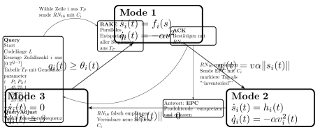
Figure 1: A hybrid system model

At Mode 1, $v_{i}\left(t\right)=v$ (the maximum speed for each agent), and

$$\cos w_{i}\left(t\right) =\frac{\frac{\partial H\left(t\right)}{\partial x_{i}\left(t\right)}}{\sqrt{\left(\frac{\partial H\left(t\right)}{\partial x_{i}\left(t\right)}\right)^{2}+\left(\frac{\partial H\left(t\right)}{\partial y_{i}\left(t\right)}\right)^{2}}},$$ (10)

$$\sin w_{i}\left(t\right) =\frac{\frac{\partial H\left(t\right)}{\partial y_{i}\left(t\right)}}{\sqrt{\left(\frac{\partial H\left(t\right)}{\partial x_{i}\left(t\right)}\right)^{2}+\left(\frac{\partial H\left(t\right)}{\partial y_{i}\left(t\right)}\right)^{2}}}\text{,}$$ (11)

where the calculations of detailed expressions for $\frac{\partial H\left(t\right)}{\partial x_{i}\left(t\right)}$ and $\frac{\partial H\left(t\right)}{\partial y_{i}\left(t\right)}$ are given in Appendix A. To ease notation, we rewrite the dynamics in (1), (2) and (3) as

$$\dot{x}_{i}\left(t\right) =f_{i}^{x}\left(t\right),$$ (12)

$$\dot{y}_{i}\left(t\right) =f_{i}^{y}\left(t\right),$$ (13)

$$\dot{q}_{i}\left(t\right) =-\alpha v^{2}.$$ (14)

Here $f_{i}^{x}\left(t\right)=v\cos w_{i}(t)$ and $f_{i}^{y}\left(t\right)=v\sin w_{i}(t)$, where the expressions of $\cos w_{i}(t)$ and $\sin w_{i}(t)$ are given by (10), and (11), respectively. Moreover, $f_{i}(s)$ in Fig. 1 is given by $f_{i}(s)=[f_{i}^{x},f_{i}^{y}]^{T}$. In other words, agent $i$ travels at the maximum speed, and the heading direction follows the gradient direction of the coverage metric with respect to agent $i$’s location. The state-of-charge of the battery monotonically decreases with rate $\alpha v^{2}$ and when it drops to a certain value, the agent switches to Mode 2.

A transition from Mode 1 to Mode 2 occurs when the guard function

$$g_{i}\left(s_{i},q_{i}\right)=q_{i}\left(t\right)-v\alpha\left\|s_{i}(t)\right\|$$ (15)

is zero, where $\left\|s_{i}(t)\right\|=\sqrt{x_{i}^{2}\left(t\right)+y_{i}^{2}\left(t\right)}$. At Mode 2, the speed $v_{i}\left(t\right)$ is determined by the scheduling algorithm used to assign an agent to the charging station and the heading direction is constant and determined by the location of agent $i$ at the time of switching from Mode 1 to Mode 2, say $\tau_{2}$. Then, the motion dynamics and the state-of-charge dynamics are:

$$\dot{x}_{i}\left(t\right) =-v_{i}\left(t\right)\frac{x_{i}\left(\tau_{2}\right)}{\left\|s_{i}(\tau_{2})\right\|},$$ (16)

$$\dot{y}_{i}\left(t\right) =-v_{i}\left(t\right)\frac{y_{i}\left(\tau_{2}\right)}{\left\|s_{i}(\tau_{2})\right\|},$$ (17)

$$\dot{q}_{i}\left(t\right) =-\alpha v_{i}^{2}\left(t\right).$$ (18)

The speed $v_{i}\left(t\right)$ in Mode 2 is piecewise constant or constant depending on which scheduling algorithm is used to resolve conflicts when multiple agents request to use the charging station at the same time, as discussed in Section IV (note that we assume no energy loss at points where the speed may experience a jump). The function $h_{i}(t)$ in Fig. 1 is a column vector containing the right-hand side of (16) and (17).

A transition from Mode 2 to Mode 3 occurs when agent $i$ arrives at the charging station and the guard function

$$g_{i}\left(s_{i}\right)=\left\|s_{i}(t)\right\|$$ (19)

is zero. At Mode 3, an agent remains at rest at the charging station, therefore, it satisfies the dynamics

$$\dot{x}_{i}\left(t\right) =0,$$ (20)

$$\dot{y}_{i}\left(t\right) =0\text{.}$$ (21)

While the agent is in charging mode, the state-of-charge dynamics are given by $\dot{q}_{i}\left(t\right)=\beta$, where $\beta\geq N\alpha v^{2}$ is the charging rate.

Finally, a transition from Mode 3 to Mode 1 occurs when the guard function $g_{i}\left(q_{i}\right)=\theta_{i}-q_{i}\left(t\right)$ is zero, where $\theta_{i}\in(0,1]$ is a controllable threshold parameter indicating the desired state-of-charge at which the agent may stop its recharging process.

Remark 3

It is worth noting that the hybrid model does not rely on a detailed energy depletion model of the state-of-charge in Mode 1. The energy consumption of sensing and communication could be included in Mode 1. When an agent switches to Mode 2, it can turn off its sensing and communication functionalities. Therefore, the energy costs in Mode 2 are only related to the agent’s speed.

The results on feasibility and rationality of the proposed hybrid model can be found in [13]. Here we only show the results on schedulability and optimality of the parameter $\theta$.

IV Scheduling Algorithms

Since the charging station can only serve one agent at a time, a scheduling algorithm is needed to resolve conflicts among agents competing over access to it. Here, we consider two scheduling policies: First-Request-First-Serve (FRFS) and Shortest-Distance-First (SDF).

IV-1 First Request First Serve

Suppose that when agent $i$ sends a charging request at $\tau_{r}^{i}$, the charging station is not reserved. Then, agent $i$ will use the maximum speed $v$ to reach the charging station. If agent $j$ sends a charging request at $\tau_{r}^{j}>\tau_{r}^{i}$, the arrival time of agent $j$ will be scheduled at $\max\{\tau_{f}^{i},\tau_{a}^{j}\}$, where $\tau_{f}^{i}$ is the time when agent $i$ finishes charging, and $\tau_{a}^{j}$ is the arrival time if agent $j$ heads to the charging station at the maximum speed. There are two different cases: $\tau_{f}^{i}<\tau_{a}^{j}$ and $\tau_{f}^{i}\geq\tau_{a}^{j}$. For the former case, there are no conflicts between agents $i$ and $j$. This is because when agent $j$ arrives at the charging station using the maximum speed, agent $i$ has already left the charging station. For the latter case, the speed of agent $j$ will be set to

$$v_{j}\left(t\right)=\frac{\left\|s_{j}(\tau_{r}^{j})\right\|}{\tau_{f}^{i}-\tau_{r}^{j}}\leq v,$$

for $\tau_{r}^{j}\leq t<\tau_{f}^{i}$. Therefore, agent $j$ will arrive at the charging station right after agent $i$ finishes charging. It is straightforward to extend the case of two agents to the case of multiple competing agents.

IV-2 Shortest Distance First

Suppose that agent $i$ sends a charging request at $\tau_{r}^{i}$. While agent $i$ is on its way to the charging station, suppose that agent $j$, which is closer to the charging station at time $\tau_{r}^{j}$, also sends a charging request. Therefore, if both agents travel at the maximum speed, agent $j$ will arrive at the charging station before agent $i$. In this case, the speed of agent $j$ is set as $v_{j}\left(t\right)=v$, and its arrival time is $\tau_{a}^{j}$. The arrival time of agent $i$ will be scheduled at $\max\{\tau^{j}_{f},\tau^{i}_{a}\}$, where $\tau_{f}^{j}$ is the leaving time of agent $j$ from the charging station and $\tau_{a}^{i}$ is the intended arrival time of agent $i$ to the charging station. Similarly, there are two different cases: $\tau_{f}^{j}<\tau_{a}^{i}$, and $\tau_{f}^{j}\geq\tau_{a}^{i}$. For the former case, there are no conflicts between agents $j$ and $i$. For the latter case, the speed of agent $i$ is set as

$$v_{i}\left(t\right)=\left\{\begin{array}[c]{cc}v&\text{for }t\in[\tau_{r}^{i},\tau_{r}^{j}),\\ \frac{\left\|s_{i}(\tau_{r}^{j})\right\|}{\tau_{f}^{j}-\tau_{r}^{j}}&\text{for }t\in[\tau_{r}^{j},\tau_{f}^{j}).\end{array}\right.$$

In this case, agent $i$ is scheduled to arrive at the charging station right after agent $j$ finishes charging. It is not difficult to extend this reasoning to the case of multiple agents: the one closer to the charging station always receives the highest priority to be served first.

V Main Results

We now address the question of selecting an optimal charging level, denoted by $\mathbf{\theta}=\left[\theta_{1},\ldots,\theta_{N}\right]$, when an agent is in the charging mode. This problem boils down to optimizing the parameter $\mathbf{\theta}$ so that the objective function in (6) is maximized. By writing explicitly the dependence on $\mathbf{\theta}$, the optimization problem becomes

$$J\left(\mathbf{\theta}\right)=\max_{\mathbf{\theta}}\frac{1}{T}\int_{0}^{T}H\left(s\left(\mathbf{\theta},t\right)\right)dt\text{.}$$

Even though $\mathbf{\theta}$ is only used in Mode 3, its optimal value affects the entire hybrid system model. By controlling $\mathbf{\theta}$, we directly control the switching times of agents from Mode 3 to Mode 1, and indirectly control the switching times of agents from Mode 1 to Mode 2. The switching times of agents from Mode 2 to Mode 3 are controlled by the proposed scheduling algorithms. Also note that the parameter $\mathbf{\theta}$ is constant. We can obtain optimal charging thresholds through off-line analysis and implement the coverage task on line by all agents in distributed fashion. We use IPA [14] to determine the optimal $\mathbf{\theta}$.

Before proceeding, we briefly review the IPA framework for general stochastic hybrid systems as presented in [14], which plays an instrumental role in obtaining the optimal dwell time of all agents at the charging station.

Let $\{\tau_{k}(\theta)\}$, $k=1,\ldots,K$, denote the occurrence times of all events in the state trajectory of a hybrid system with dynamics $\dot{x}\ =\ f_{k}(x,\theta,t)$ over an interval $[\tau_{k}(\theta),\tau_{k+1}(\theta))$, where $\theta\in\Theta$ is some parameter vector and $\Theta$ is a given compact, convex set. For convenience, we set $\tau_{0}=0$ and $\tau_{K+1}=T$. We use the Jacobian matrix notation: $x^{\prime}(t)\equiv\frac{\partial x(\theta,t)}{\partial\theta}$ and $\tau_{k}^{\prime}\equiv\frac{\partial\tau_{k}(\theta)}{\partial\theta}$, for all state and event time derivatives. It is shown in [14] that

$$\frac{d}{dt}x^{\prime}(t)=\frac{\partial f_{k}(t)}{\partial x}x^{\prime}(t)+\frac{\partial f_{k}(t)}{\partial\theta},$$ (22)

for $t\in[\tau_{k},\tau_{k+1})$ with boundary condition:

$$x^{\prime}(\tau_{k}^{+})=x^{\prime}(\tau_{k}^{-})+[f_{k-1}(\tau_{k}^{-})-f_{k}(\tau_{k}^{+})]\tau_{k}^{\prime},$$ (23)

for $k=0,...,K$. In order to complete the evaluation of $x^{\prime}(\tau_{k}^{+})$ in (23), we need to determine $\tau_{k}^{\prime}$. We classify events into two categories. An event is exogenous if it causes a discrete state transition at time $\tau_{k}$ independent of the controllable vector $\theta$ and, therefore, satisfies $\tau_{k}^{\prime}=0$. Otherwise, the event is endogenous and there exists a continuously differentiable function $g_{k}:\mathbb{R}^{n}\times\Theta\rightarrow\mathbb{R}$ such that $\tau_{k}\ =\ \min\{t>\tau_{k-1}\ :\ g_{k}\left(x\left(\theta,t\right),\theta\right)=0\}$ and

$$\tau_{k}^{\prime}=-[\frac{\partial g_{k}}{\partial x}f_{k}(\tau_{k}^{-})]^{-1}(\frac{\partial g_{k}}{\partial\theta}+\frac{\partial g_{k}}{\partial x}x^{\prime}(\tau_{k}^{-}))$$ (24)

as long as $\frac{\partial g_{k}}{\partial x}f_{k}(\tau_{k}^{-})\neq 0$ (details may be found in [14]).

Denote the time-varying cost along a given trajectory as $L(x,\theta,t)$, so the cost in the $k$-th inter-event interval is $J_{k}(x,\theta)=\int_{\tau_{k}}^{\tau_{k+1}}L(x,\theta,t)dt$ and the total cost is $J(x,\theta)=\sum_{k=0}^{K}J_{k}(x,\theta)$. Differentiating and applying the Leibniz rule with the observation that all terms of the form $L(x(\tau_{k}),\theta,\tau_{k})\tau_{k}^{\prime}$ are mutually canceled with $\tau_{0}=0,\tau_{K+1}=T$ fixed, we obtain

$$\frac{\partial J(x,\theta)}{\partial\theta} =\sum_{k=0}^{K}\frac{\partial}{\partial\theta}\int_{\tau_{k}}^{\tau_{k+1}}L(x,\theta,t)dt$$

$$=\sum_{k=0}^{K}\int_{\tau_{k}}^{\tau_{k+1}}\frac{\partial L(x,\theta,t)}{\partial x}x^{\prime}(t)+\frac{\partial L(x,\theta,t)}{\partial\theta}dt.$$ (25)

Now let us return to our problem and define the following notations

$$\tau^{\prime}_{k}=\frac{\partial\tau_{k}(\theta)}{\partial\theta},\quad\mathbf{x}^{\prime}_{i}=\frac{\partial x_{i}(\theta)}{\partial\theta},\quad\mathbf{y}^{\prime}_{i}=\frac{\partial y_{i}(\theta)}{\partial\theta}$$

which are row vectors, and

$$\frac{\partial\mathbf{x}\left(\theta,t\right)}{\partial\mathbf{\theta}} =\left[\mathbf{x}_{1}^{\prime}\left(\theta,t\right)^{T},\cdots,\mathbf{x}_{N}^{\prime}\left(\theta,t\right)^{T}\right]^{T}\text{,}$$

$$\frac{\partial\mathbf{y}\left(\theta,t\right)}{\partial\mathbf{\theta}} =\left[\mathbf{y}_{1}^{\prime}\left(\theta,t\right)^{T},\cdots,\mathbf{y}_{N}^{\prime}\left(\theta,t\right)^{T}\right]^{T}\text{,}$$

are matrices.

Let us assume that all agents start with the battery level

$$q_{i}\left(0\right)>v\alpha\left\|s_{i}\left(0\right)\right\|\text{,}$$

for $i=1,\ldots,N,$ that is, all agents start with Mode 1.

For $t\in\left[\tau_{1},\tau_{2}\right)$, applying (22) to (12) and (13) yields that

$$\frac{d}{dt}\mathbf{x}_{i}^{\prime}\left(\theta,t\right) =v\frac{\partial\cos w_{i}\left(t\right)}{\partial\mathbf{x}\left(\theta,t\right)}\frac{\partial\mathbf{x}\left(\theta,t\right)}{\partial\mathbf{\theta}}+v\frac{\partial\cos w_{i}\left(t\right)}{\partial\mathbf{y}\left(\theta,t\right)}\frac{\partial\mathbf{y}\left(\theta,t\right)}{\partial\mathbf{\theta}},$$ (26)

$$\frac{d}{dt}\mathbf{y}_{i}^{\prime}\left(\theta,t\right) =v\frac{\partial\sin w_{i}\left(t\right)}{\partial\mathbf{x}\left(\theta,t\right)}\frac{\partial\mathbf{x}\left(\theta,t\right)}{\partial\mathbf{\theta}}+v\frac{\partial\sin w_{i}\left(t\right)}{\partial\mathbf{y}\left(\theta,t\right)}\frac{\partial\mathbf{y}\left(\theta,t\right)}{\partial\mathbf{\theta}},$$ (27)

where the detailed calculations of $\frac{\partial\cos w_{i}\left(t\right)}{\partial\mathbf{x}\left(\theta,t\right)}$, $\frac{\partial\cos w_{i}\left(t\right)}{\partial\mathbf{y}\left(\theta,t\right)}$, $\frac{\partial\sin w_{i}\left(t\right)}{\partial\mathbf{x}\left(\theta,t\right)}$, and $\frac{\partial\sin w_{i}\left(t\right)}{\partial\mathbf{y}\left(\theta,t\right)}$ can be founded in Appendix B. Note that for agents $j\notin\mathcal{N}_{i}$,

$$\frac{\partial\cos w_{i}\left(t\right)}{\partial x_{j}\left(t\right)}=0,\quad\frac{\partial\sin w_{i}\left(t\right)}{\partial x_{j}\left(t\right)}=0.$$

For the state-of-charge, we have

$$\frac{d}{dt}\mathbf{q}_{i}^{\prime}\left(\theta,t\right)=\mathbf{0},$$

by applying (22) to (14), which implies that $\mathbf{q}_{i}^{\prime}\left(\theta,\tau_{2}^{-}\right)=\mathbf{q}_{i}^{\prime}\left(\theta,\tau_{1}^{+}\right)$. By solving the differential equations (26) and (27), we can obtain $\mathbf{x}_{i}^{\prime}\left(\theta,\tau_{2}^{-}\right)$ and $\mathbf{y}_{i}^{\prime}\left(\theta,\tau_{2}^{-}\right)$.

At $\tau_{2},$ the guard condition

$$g_{i}\left(x_{i}\left(\theta,\tau_{2}\right),y_{i}\left(\theta,\tau_{2}\right),q_{i}\left(\theta,\tau_{2}\right)\right)$$

$$= q_{i}^{2}\left(\theta,\tau_{2}\right)-v^{2}\alpha^{2}\|s_{i}\left(\theta,\tau_{2}\right)\|^{2}=0.$$

Note that we use an equivalent form of (15) by squaring both terms for an easier calculation of derivatives. This is an endogenous event. By applying (24) to the above guard function and the dynamics in (12), (13) and (14), we have

$$\mathbf{\tau}_{2}^{\prime}=\frac{q_{i}\left(\tau_{2}\right)\mathbf{q}_{i}^{\prime}\left(\tau_{2}^{-}\right)-v^{2}\alpha^{2}\left[x_{i}\left(\tau_{2}\right)\mathbf{x}_{i}^{\prime}\left(\tau_{2}^{-}\right)+y_{i}\left(\tau_{2}\right)\mathbf{y}_{i}^{\prime}\left(\tau_{2}^{-}\right)\right]}{\alpha v^{2}q_{i}\left(\tau_{2}\right)+v^{3}\alpha^{2}\left[x_{i}\left(\tau_{2}\right)\cos w_{i}\left(\tau_{2}^{-}\right)+y_{i}\left(\tau_{2}\right)\sin w_{i}\left(\tau_{2}^{-}\right)\right]}$$

with the boundary conditions

$$\mathbf{q}_{i}^{\prime}\left(\tau_{2}^{+}\right) =\mathbf{q}_{i}^{\prime}\left(\tau_{2}^{-}\right)+\alpha\left[v_{i}^{2}\left(\tau_{2}^{+}\right)-v^{2}\right]\mathbf{\tau}_{2}^{\prime}$$

$$\mathbf{x}_{i}^{\prime}\left(\tau_{2}^{+}\right) =\mathbf{x}_{i}^{\prime}\left(\tau_{2}^{-}\right)+\left[v\cos w_{i}\left(\tau_{2}^{-}\right)-v_{i}\left(\tau_{2}^{+}\right)\cos w_{i}\left(\tau_{2}^{+}\right)\right]\mathbf{\tau}_{2}^{\prime},$$

$$\mathbf{y}_{i}^{\prime}\left(\tau_{2}^{+}\right) =\mathbf{y}_{i}^{\prime}\left(\tau_{2}^{-}\right)+\left[v\sin w_{i}\left(\tau_{2}^{-}\right)-v_{i}\left(\tau_{2}^{+}\right)\sin w_{i}\left(\tau_{2}^{+}\right)\right]\mathbf{\tau}_{2}^{\prime},$$

which are obtained by applying (23) to the dynamics in (16), (17) and (18).

Remark 4

Irrespective of the scheduling algorithm, if agent $i$ is the first to request charging in the current queue, then $v_{i}\left(\tau_{2}^{+}\right)=v$, and $\textbf{q}_{i}^{\prime}\left(\theta,\tau_{2}^{+}\right)=\textbf{q}_{i}^{\prime}\left(\theta,\tau_{2}^{-}\right)=\textbf{q}_{i}^{\prime}\left(\theta,\tau_{1}^{+}\right)$.

In Mode 2, the right-hand sides of (16), (17), and (18) are constant or piecewise constant depending on the scheduling algorithm. Therefore, we have

$$\frac{d}{dt}\mathbf{x}_{i}^{\prime}\left(\theta,t\right)=0,\quad\frac{d}{dt}\mathbf{y}_{i}^{\prime}\left(\theta,t\right)=0,$$

$$\frac{d}{dt}\mathbf{q}_{i}^{\prime}\left(\theta,t\right)=0,$$

according to (22). It is easy to see that

$$\mathbf{x}_{i}^{\prime}\left(\theta,\tau_{3}^{-}\right) =\mathbf{x}_{i}^{\prime}\left(\theta,\tau_{2}^{+}\right),$$ (28)

$$\mathbf{y}_{i}^{\prime}\left(\theta,\tau_{3}^{-}\right) =\mathbf{y}_{i}^{\prime}\left(\theta,\tau_{2}^{+}\right),$$ (29)

$$\mathbf{q}_{i}^{\prime}\left(\theta,\tau_{3}^{-}\right) =\mathbf{q}_{i}^{\prime}\left(\theta,\tau_{2}^{+}\right).$$ (30)

In the SDF scheduling algorithm, the velocity of agent $i$ may be adjusted due to the competition to the charging station. This is the case when agent $j$, which is closer to the charing station than agent $i$, requests for the charging service. Such events are independent of $\theta$ and are, therefore, treated as exogenous events. In Mode 2, the relationships (28), (29), and (30) hold independent of the scheduling methods, and the number of exogenous events.

At time $\tau_{3}$, the guard function $g_{i}\left(x_{i}\left(\theta,\tau_{3}\right),y_{i}\left(\theta,\tau_{3}\right)\right)=\|s_{i}\left(\tau_{3}\right)\|^{2}=0$. Again, an equivalent form of the guard function (19) is used by squaring the term for an easier calculation of derivatives. This is an endogenous event. According to (24), we can calculate

$$\mathbf{\tau}_{3}^{\prime}=-\frac{x_{i}\left(\theta,\tau_{3}\right)\mathbf{x}_{i}^{\prime}\left(\theta,\tau_{3}^{-}\right)+y_{i}\left(\theta,\tau_{3}\right)\mathbf{y}_{i}^{\prime}\left(\theta,\tau_{3}^{-}\right)}{x_{i}\left(\theta,\tau_{3}\right)v_{i}\left(\tau_{3}^{-}\right)\cos w_{i}\left(\tau_{3}^{-}\right)+y_{i}\left(\theta,\tau_{3}\right)v_{i}\left(\tau_{3}^{-}\right)\sin w_{i}\left(\tau_{3}^{-}\right)}$$

based on the dynamics (16), (17) and (18) and the boundary conditions are

$$\mathbf{x}_{i}^{\prime}\left(\theta,\tau_{3}^{+}\right) =\mathbf{x}_{i}^{\prime}\left(\theta,\tau_{3}^{-}\right)+v_{i}\left(\tau_{3}^{-}\right)\cos w_{i}\left(\tau_{3}^{-}\right)\mathbf{\tau}_{3}^{\prime}$$

$$\mathbf{y}_{i}^{\prime}\left(\theta,\tau_{3}^{+}\right) =\mathbf{y}_{i}^{\prime}\left(\theta,\tau_{3}^{-}\right)+v_{i}\left(\tau_{3}^{-}\right)\sin w_{i}\left(\tau_{3}^{-}\right)\mathbf{\tau}_{3}^{\prime}$$

$$\mathbf{q}_{i}^{\prime}\left(\tau_{3}^{+}\right) =\mathbf{q}_{i}^{\prime}\left(\theta,\tau_{3}^{-}\right)-\left[\alpha v_{i}^{2}\left(\tau_{3}^{-}\right)+\beta\right]\mathbf{\tau}_{3}^{\prime}$$

by applying (23) to the dynamics in (20), (21) and (5).

Remark 5

When calculating $\mathbf{\tau}_{3}^{\prime}$, we find that both the numerator and denominator are zero due to $x_{i}\left(\theta,\tau_{3}\right)=y_{i}\left(\theta,\tau_{3}\right)=0$. In this case, the value of $\mathbf{\tau}_{3}^{\prime}$ is calculated according to its limit in the direction $w_{i}(\mathbf{\tau}_{3}^{-})$. Let us put $x_{i}$ and $y_{i}$ in the polar coordinate, then $x_{i}=r\cos w_{i}\left(\tau_{3}^{-}\right)$ and $y_{i}=r\sin w_{i}\left(\tau_{3}^{-}\right)$. Replacing $x_{i}$ and $y_{i}$ in $\mathbf{\tau}_{3}^{\prime}$, it becomes

$$\mathbf{\tau}_{3}^{\prime} =-\lim_{r\rightarrow 0}\frac{r\cos w_{i}\left(\tau_{3}^{-}\right)\mathbf{x}_{i}^{\prime}\left(\theta,\tau_{3}^{-}\right)+r\sin w_{i}\left(\tau_{3}^{-}\right)\mathbf{y}_{i}^{\prime}\left(\theta,\tau_{3}^{-}\right)}{rv_{i}\left(\tau_{3}^{-}\right)\cos w_{i}^{2}\left(\tau_{3}^{-}\right)+rv_{i}\left(\tau_{3}^{-}\right)\sin w_{i}^{2}\left(\tau_{3}^{-}\right)}$$

$$=-\frac{\cos w_{i}\left(\tau_{3}^{-}\right)\mathbf{x}_{i}^{\prime}\left(\theta,\tau_{3}^{-}\right)+\sin w_{i}\left(\tau_{3}^{-}\right)\mathbf{y}_{i}^{\prime}\left(\theta,\tau_{3}^{-}\right)}{v_{i}\left(\tau_{3}^{-}\right)}.$$

Note that in Mode 2, agents do not change their direction and $w_{i}\left(\tau_{3}^{-}\right)=w_{i}\left(\tau_{2}^{+}\right)$.

In Mode 3, during the cycle $\left[\tau_{3},\tau_{1}\right),$ we can obtain

$$\frac{d}{dt}\mathbf{x}_{i}^{\prime}\left(\theta,t\right)=0,\quad\frac{d}{dt}\mathbf{y}_{i}^{\prime}\left(\theta,t\right)=0,\quad\frac{d}{dt}\mathbf{q}_{i}^{\prime}\left(\theta,t\right)=0$$

by applying (22) to the dynamic equations (20), (21) and (5). Therefore, it is easy to calculate

$$\mathbf{x}_{i}^{\prime}\left(\theta,\tau_{1}^{-}\right) =\mathbf{x}_{i}^{\prime}\left(\theta,\tau_{3}^{+}\right),\quad\mathbf{y}_{i}^{\prime}\left(\theta,\tau_{1}^{-}\right)=\mathbf{y}_{i}^{\prime}\left(\theta,\tau_{3}^{+}\right)$$

$$\mathbf{q}_{i}^{\prime}\left(\theta,\tau_{1}^{-}\right) =\mathbf{q}_{i}^{\prime}\left(\theta,\tau_{3}^{+}\right)\text{.}$$

At time $\tau_{1}$, the threshold

$$g_{i}\left(q_{i}\left(\theta,\tau_{1}\right)\right)=q_{i}\left(\theta,\tau_{1}\right)-\theta_{i}=0.$$

This is an endogenous event. We can obtain

$$\mathbf{\tau}_{1}^{\prime}=\frac{1-\textbf{q}_{i}^{\prime}\left(\theta,\tau_{1}^{-}\right)}{\beta},$$

and the boundary conditions

$$\mathbf{x}_{i}^{\prime}\left(\theta,\tau_{1}^{+}\right) =\mathbf{x}_{i}^{\prime}\left(\theta,\tau_{1}^{-}\right)-v\cos w_{i}\left(\tau_{1}^{+}\right)\mathbf{\tau}_{1}^{\prime}$$

$$\mathbf{y}_{i}^{\prime}\left(\theta,\tau_{1}^{+}\right) =\mathbf{y}_{i}^{\prime}\left(\theta,\tau_{1}^{-}\right)-v\sin w_{i}\left(\tau_{1}^{+}\right)\mathbf{\tau}_{1}^{\prime}$$

$$\mathbf{q}_{i}^{\prime}\left(\theta,\tau_{1}^{+}\right) =\mathbf{q}_{i}^{\prime}\left(\theta,\tau_{1}^{-}\right)+\left(\beta+\alpha v^{2}\right)\mathbf{\tau}_{1}^{\prime}\text{,}$$

according to (24) and (23), respectively, based on the dynamics in (20), (21), (5), (12), (13) and (14). Now the IPA derivative of $dJ/d\theta$ can be obtained by taking derivatives of $J(\theta)$ with respective to $\theta$ as shown in (25):

$$\frac{dJ}{d\theta}=\sum_{k=0}^{l}\frac{d}{d\theta}\int_{t_{k}}^{t_{k+1}}H_{k}\left(s,\theta,t\right)dt$$

and applying the Leibnitz rule we obtain, for every $k=0,\ldots,l,$

$$\frac{d}{d\theta}\int_{t_{k}}^{t_{k+1}}H_{k}\left(s,\theta,t\right)dt$$

$$= \int_{t_{k}}^{t_{k+1}}\left[\frac{\partial H_{k}\left(s,\theta,t\right)}{\partial\mathbf{x}}\mathbf{x}^{\prime}+\frac{\partial H_{k}\left(s,\theta,t\right)}{\partial\mathbf{y}}\mathbf{y}^{\prime}\right]dt$$

$$+H_{k}\left(s\left(t_{k+1}\right),\theta,t_{k+1}\right)\mathbf{t}_{k+1}^{\prime}-H_{k}\left(s\left(t_{k}\right),\theta,t_{k}\right)\mathbf{t}_{k}^{\prime}$$

where $t_{k}$ are event times of any agents, $t_{0}=0$ and $t_{l}=T$. The parameter $\theta$ is updated as

$$\theta_{n+1}=\theta_{n}+\lambda_{n}\frac{dJ(\theta_{n})}{d\theta_{n}},$$ (31)

where $\{\lambda_{n}\}$ is a step size sequence.

VI SIMULATION RESULTS

In this section, we illustrate the optimization process in (31), and compare the performance by using different scheduling algorithms (FRFS, and SDF).

The mission space is a 60 by 50 rectangular area without obstacles. We consider a team of four agents with initial locations (2,2), (4,4), (6,6) and (8,8). The initial state-of-charge variables are randomly generated, which are $97\%$, $48\%$, $71\%$, and $46\%$, respectively. The maximum speed is $v=5$, and the sensing range $\delta_{i}=22$ for all $i=1,\ldots,4$. The parameter $\alpha=0.0001$, and $\beta=4\alpha v^{2}=0.01$. Figures 2 and 3 show the evolution of $\theta$ under the FRFS and SDF scheduling algorithms, respectively, where the step size sequence $\{\lambda_{n}\}$ over iterations $n=0,1,\ldots$, is chosen as $\{(\|\frac{dJ(\theta_{n})}{d\theta_{n}}\|n^{\frac{3}{2}})^{-1}\}$. It can be seen from both figures that it is optimal to fully charge the battery for both scheduling algorithms. The simulation runs for $T=5400$ by considering the optimal $\theta=1$. The comparison of the coverage performance between different scheduling algorithms is depicted in Fig. 4. The coverage performance is $J(\theta)=186407$ for FRFS, and $J(\theta)=186095$ for SDF, respectively. The difference between the performance of the two scheduling algorithms is within $0.1\%$. Therefore, no general conclusions can be drawn on which scheduling algorithm is better, even though we might expect SDF to be preferable because it uses the distance information compared to FRFS.

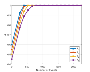
Figure 2: The evolution of $\theta$ under the FRFS scheduling method

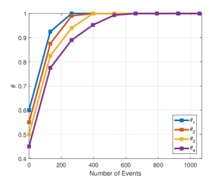
Figure 3: The evolution of $\theta$ under the SDF scheduling method

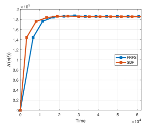
Figure 4: The comparison of performance using different scheduling algorithms

A visual interactive simulation can be found at http://www.bu.edu/codes/simulations/Coverage_ADHS. Interested readers are encouraged to interact with the simulation by choosing different scheduling algorithms, as well as adjusting parameters such as the number of agents $N$, the sensing range $\delta_{i}$, or the maximum speed $v$.

VII CONCLUSIONS

A hybrid system model is proposed to capture the behavior of multiple agents cooperatively solving an optimal coverage problem under energy depletion and repletion constraints. The proposed model links each agent’s coverage, to-charging, and in-charging modes so as to form a cycle and the guard conditions are designed to maximize the coverage performance over a finite time horizon as well as to ensure that the agents never run out of energy. Full repletion is optimal to maximize the coverage objective function as shown by numerical calculations using IPA; and a theoretical proof is the subject of ongoing research. We are also working on the inclusion of energy expended for communication among agents (see Remark 1). Finally, when obstacles are present in the mission space, finding optimal trajectories for agents in Mode 2 is a challenging task that we plan to address in future work.

APPENDIX

VII-A Calculation of the Gradient

To find the heading direction of agent $i$, we need to calculate the gradient of $H\left(\mathbf{s}\right)$ at point $(x_{i},y_{i})$, which is

$$\nabla H\left(s_{i}\right)=\left[\frac{\partial H}{\partial x_{i}},\frac{\partial H}{\partial y_{i}}\right]^{T}\text{.}$$

According to [19], we can calculate the gradient as

$$\frac{\partial H}{\partial x_{i}}=\iint\nolimits_{\Omega}\frac{\partial P}{\partial x_{i}}+\int_{\partial\Omega}P\left(\frac{\partial x}{\partial x_{i}}dy-\frac{\partial y}{\partial x_{i}}dx\right),$$

where the integration in the second term is done in the counterclockwise direction over the boundary of $\Omega$. Recalling the expressions of (7) and (8), we have

$$\int_{\partial\Omega}P\left(\frac{\partial x}{\partial x_{i}}dy-\frac{\partial y}{\partial x_{i}}dx\right)=0\text{.}$$

This is because when $\left(x,y\right)\in\partial\Omega\cap\partial\Omega_{i}$, $P=0$; when $\left(x,y\right)\in\partial\Omega\backslash\partial\Omega_{i}$,

$$\frac{\partial x}{\partial x_{i}}=\frac{\partial y}{\partial x_{i}}=0\text{.}$$

Therefore, we can obtain

$$\frac{\partial H}{\partial x_{i}}=\iint\limits_{\Omega_{i}}\frac{2\left(x-x_{i}\right)}{\delta_{i}^{2}}\prod\limits_{j\in\mathcal{N}_{i}}\left(1-p_{j}\right)dxdy.$$ (32)

Similarly, we have

$$\frac{\partial H}{\partial y_{i}}=\iint\limits_{\Omega_{i}}\frac{2\left(y-y_{i}\right)}{\delta_{i}^{2}}\prod\limits_{j\in\mathcal{N}_{i}}\left(1-p_{j}\right)dxdy.$$ (33)

Remark 6

When the sensing range $\Omega_{i}$ of agent $i$ is blocked by the boundary, the gradient can be derived similarly using a simple projection onto the feasible mission space. The detailed calculations for this case are thus not shown here.

VII-B Derivative of the Gradient

Here we discuss the calculations of $\frac{\partial\cos w_{i}}{\partial\mathbf{x}}$, and the formulas for $\frac{\partial\cos w_{i}}{\partial\mathbf{y}}$, $\frac{\partial\sin w_{i}}{\partial\mathbf{x}}$, $\frac{\partial\sin w_{i}}{\partial\mathbf{y}}$ can be derived similarly.

Recalling the definition of $\cos w_{i}$ in (10), we take the derivative of $\cos w_{i}$ with respect to $x_{i}$, and have

$$\frac{\partial\cos w_{i}}{\partial x_{i}} =\frac{\left\|\nabla H\left(s_{i}\right)\right\|\frac{\partial^{2}H}{\partial x_{i}^{2}}-\frac{\partial H}{\partial x_{i}}\frac{\frac{\partial H}{\partial x_{i}}\frac{\partial^{2}H}{\partial x_{i}^{2}}+\frac{\partial H}{\partial y_{i}}\frac{\partial^{2}H}{\partial x_{i}\partial y_{i}}}{\left\|\nabla H\left(s_{i}\right)\right\|}}{\left\|\nabla H\left(s_{i}\right)\right\|^{2}}$$

$$=\frac{\frac{\partial^{2}H}{\partial x_{i}^{2}}}{\left\|\nabla H\left(s_{i}\right)\right\|}-\frac{\cos w_{i}\left(t\right)\left(\frac{\partial H}{\partial x_{i}}\frac{\partial^{2}H}{\partial x_{i}^{2}}+\frac{\partial H}{\partial y_{i}}\frac{\partial^{2}H}{\partial x_{i}\partial y_{i}}\right)}{\left\|\nabla H\left(s_{i}\right)\right\|^{2}}.$$

In order to obtain $\frac{\partial\cos w_{i}}{\partial\mathbf{x}},$ we need to calculate $\frac{\partial^{2}H}{\partial x_{i}^{2}}$ and $\frac{\partial^{2}H}{\partial y_{i}\partial x_{i}}$, which will be given as follows. Taking the partial derivative of (32) with respect to $x_{i}$, we have

$$\frac{\partial^{2}H}{\partial x_{i}^{2}} =-\frac{2}{\delta_{i}^{2}}\iint\limits_{\Omega_{i}}\prod\limits_{j\in\mathcal{N}_{i}}\left(1-p_{j}\right)dxdy$$

$$+\int_{y_{i}-\delta_{i}}^{y_{i}+\delta_{i}}\frac{2\sqrt{\delta_{i}^{2}-\left(y-y_{i}\right)^{2}}}{\delta_{i}^{2}}\prod\nolimits_{j\in\mathcal{N}_{i}}\left[1-\hat{p}_{j}\right]dy$$

$$+\int_{y_{i}-\delta_{i}}^{y_{i}+\delta_{i}}\frac{2\sqrt{\delta_{i}^{2}-\left(y-y_{i}\right)^{2}}}{\delta_{i}^{2}}\prod\nolimits_{j\in\mathcal{N}_{i}}\left[1-\check{p}_{j}\right]dy,$$

where

$$\hat{p}_{j} =p_{j}\left(x_{i}+\sqrt{\delta_{i}^{2}-\left(y-y_{i}\right)^{2}},y,x_{i},y_{i}\right),$$

$$\check{p}_{j} =p_{j}\left(x_{i}-\sqrt{\delta_{i}^{2}-\left(y-y_{i}\right)^{2}},y,x_{i},y_{i}\right),$$

and the definition of $p_{j}$ is given in (8).

Similarly, we have

$$\frac{\partial^{2}H}{\partial x_{i}\partial y_{i}}$$

$$= \frac{\partial}{\partial y_{i}}\int_{x_{i}-\delta_{i}}^{x_{i}+\delta_{i}}\int_{y_{i}-\sqrt{\delta_{i}^{2}-\left(x-x_{i}\right)^{2}}}^{y_{i}+\sqrt{\delta_{i}^{2}-\left(x-x_{i}\right)^{2}}}\frac{2\left(x-x_{i}\right)}{\delta_{i}^{2}}\prod\limits_{j\in\mathcal{N}_{i}}\left(1-p_{j}\right)dydx$$

$$= \int_{x_{i}-\delta_{i}}^{x_{i}+\delta_{i}}\frac{2\left(y_{i}-x_{i}+\sqrt{\delta_{i}^{2}-\left(x-x_{i}\right)^{2}}\right)}{\delta_{i}^{2}}\prod\nolimits_{j\in\mathcal{N}_{i}}\left(1-\tilde{p}_{j}\right)dx$$

$$-\int_{x_{i}-\delta_{i}}^{x_{i}+\delta_{i}}\frac{2\left(y_{i}-x_{i}-\sqrt{\delta_{i}^{2}-\left(x-x_{i}\right)^{2}}\right)}{\delta_{i}^{2}}\prod\nolimits_{j\in\mathcal{N}_{i}}\left(1-\breve{p}_{j}\right)dx$$

where

$$\tilde{p}_{j} =p_{j}\left(x,y_{i}+\sqrt{\delta_{i}^{2}-\left(x-x_{i}\right)^{2}},x_{i},y_{i}\right),$$

$$\breve{p}_{j} =p_{j}\left(x,y_{i}-\sqrt{\delta_{i}^{2}-\left(x-x_{i}\right)^{2}},x_{i},y_{i}\right).$$

References

• [1] M. Zhong and C. G. Cassandras, “Distributed coverage control and data collection with mobile sensor networks,” IEEE Trans. Autom. Control, vol. 56, no. 10, pp. 2445–2455, 2011.
• [2] N. E. Leonard and A. Olshevsky, “Nonuniform coverage control on the line,” IEEE Trans. Autom. Control, vol. 58, no. 11, pp. 2743–2755, 2013.
• [3] Y. Kantaros, M. Thanou, and A. Tzes, “Distributed coverage control for concave areas by a heterogeneous robot swarm with visibility sensing constraints,” Automatica, vol. 53, pp. 195 – 207, 2015.
• [4] Z. Tang and U. Ozguner, “Motion planning for multitarget surveillance with mobile sensor agents,” IEEE Transactions on Robotics, vol. 21, no. 5, pp. 898–908, 2005.
• [5] S. L. Smith, M. Schwager, and D. Rus, “Persistent robotic tasks: Monitoring and sweeping in changing environments,” IEEE Transactions on Robotics, vol. 28, no. 2, pp. 410–426, 2012.
• [6] S. Meguerdichian, F. Koushanfar, M. Potkonjak, and M. B. Srivastava, “Coverage problems in wireless ad-hoc sensor networks,” in Proceedings IEEE INFOCOM, vol. 3, 2001, pp. 1380–1387.
• [7] J. Cortes, S. Martinez, T. Karatas, and F. Bullo, “Coverage control for mobile sensing networks,” IEEE Transactions on Robotics and Automation, vol. 20, no. 2, pp. 243–255, 2004.
• [8] X. Sun, C. G. Cassandras, and K. Gokbayrak, “Escaping local optima in a class of multi-agent distributed optimization problems: A boosting function approach,” in Proc. IEEE Conf. on Decision and Control, 2014, pp. 3701–3706.
• [9] Z. Zhang, E. K. P. Chong, A. Pezeshki, and W. Moran, “String submodular functions with curvature constraints,” IEEE Trans. Autom. Control, vol. 61, no. 3, pp. 601–616, 2016.
• [10] X. Sun, C. G. Cassandras, and X. Meng, “A submodularity-based approach for multi-agent optimal coverage problems,” in Proc. IEEE Conf. on Decision and Control, 2017, pp. 4082–4087.
• [11] K. Leahy, D. Zhou, C.-I. Vasile, K. Oikonomopoulos, M. Schwager, and C. Belta, “Persistent surveillance for unmanned aerial vehicles subject to charging and temporal logic constraints,” Autonomous Robots, vol. 40, no. 8, pp. 1363–1378, 2016.
• [12] D. Aksaray, C.-I. Vasile, and C. Belta, “Dynamic routing of energy-aware vehicles with temporal logic constraints,” in Proc. IEEE International Conf. Robotics and Automation.   IEEE, 2016, pp. 3141–3146.
• [13] X. Meng, A. Houshmand, and C. G. Cassandras, “Hybrid system modeling of multi-agent coverage problems with energy depletion and repletion,” in Proceedings IFAC Conf. Analysis and Design of Hybrid Systems, to appear.
• [14] C. G. Cassandras, Y. Wardi, C. G. Panayiotou, and C. Yao, “Perturbation analysis and optimization of stochastic hybrid systems,” European Journal of Control, vol. 16, no. 6, pp. 642 – 661, 2010.
• [15] T. Setter and M. Egerstedt, “Energy-constrained coordination of multi-robot teams,” IEEE Trans. Control Syst. Technol., vol. PP, no. 99, pp. 1–7, 2016.
• [16] D. M. Stipanovic, C. Valicka, C. J. Tomlin, and T. R. Bewley, “Safe and reliable coverage control,” Numerical Algebra, Control and Optimization, vol. 3, no. 1, pp. 31–48, 2013.
• [17] D. Panagou, D. M. Stipanović, and P. G. Voulgaris, “Dynamic coverage control in unicycle multi-robot networks under anisotropic sensing,” Frontiers in Robotics and AI, vol. 2, p. 3, 2015.
• [18] X. Lin and C. G. Cassandras, “An optimal control approach to the multi-agent persistent monitoring problem in two-dimensional spaces,” IEEE Trans. Autom. Control, vol. 60, no. 6, pp. 1659–1664, 2015.
• [19] H. Flanders, “Differentiation under the integral sign,” The American Mathematical Monthly, vol. 80, no. 6, pp. 615–627, 1973.