Deep Global Model Reduction Learning

Abstract

In this paper, we combine deep learning concepts and some proper orthogonal decomposition (POD) model reduction methods for predicting flow in heterogeneous porous media. Nonlinear flow dynamics is studied, where the dynamics is regarded as a multi-layer network. The solution at the current time step is regarded as a multi-layer network of the solution at the initial time and input parameters. As for input, we consider various sources, which include source terms (well rates), permeability fields, and initial conditions. We consider the flow dynamics, where the solution is known at some locations and the data is integrated to the flow dynamics by modifying the reduced-order model. This approach allows modifying the reduced-order formulation of the problem. Because of the small problem size, limited observed data can be handled. We consider enriching the observed data using the computational data in deep learning networks. The basis functions of the global reduced order model are selected such that the degrees of freedom represent the solution at observation points. This way, we can avoid learning basis functions, which can also be done using neural networks. We present numerical results, where we consider channelized permeability fields, where the network is constructed for various channel configurations. Our numerical results show that one can achieve a good approximation using forward feed maps based on multi-layer networks.

1 Introduction

Mathematical models are widely used to describe the underlying physical process in science and engineering disciplines. In many real-life applications, for instance, large-scale dynamical systems and control systems, the mathematical models are of high complexity and numerical simulations in high dimensional systems become challenging. Model order reduction (MOR) is a useful technique in obtaining reasonable approximations with a significantly reduced computational cost of such problems. Through obtaining dominant modes, the dimension of the associated state space is reduced and an approximation of the original model with acceptable accuracy is computed. Proper Orthogonal Decomposition (POD) has been used in numerical approximations for dynamic systems [19, 22]. Recently, POD has been applied to flow problems in porous media with high contrasts and heterogeneities [15, 14, 37, 2, 21, 32, 3, 11, 33]. The objective of this work is to develop data-driven POD reduced-order models for such problems using advancements of machine learning.

A main difficulty of model order reduction is nonlinear problems. In such problems, modes have to be re-trained or computed in an online process [12, 1, 6], which is, in many cases, computationally expensive. Moreover, in cases with observed data, the off-line computed modes may not honor the data. In this work, our goal is to develop an appropriate model reduction , which overcomes the difficulties of nonlinear problems and data-present problems. We discuss the design of proper orthogonal decomposition (POD) modes, where the degrees of freedom have physical meanings. In particular, they represent the values of the solution at fixed pre-selected locations. This allows working with POD coefficients without constructing POD basis functions in cases relevant to reservoir engineering.

Recently, deep learning has attracted a lot attention ([17, 25, 30]). Deep Neural Network (DNN) is at the core of deep learning, and is a computing system inspired by the brain’s architecture. DNN has showed its power in tackling some complex and challenging computer vision tasks, such as classifying a huge number of images, recognizing speech and so on. A deep neural network usually consists of an input layer, an output layer and multiple intermediate hidden layers, with several neurons in each layer. In the learning process, each layer transforms its input data into a little more abstract representation and transfers the signal to the next layer. Some activation functions, acting as the nonlinear transformation on the input signal, are applied to determine whether a neuron is activated or not.

There have been many works discovering the expressivity of deep neural nets theoretically [8, 20, 7, 31, 28, 18]. The universal approximation property of neural networks has been investigated in a lot of recent studies. It has been shown that deep networks are powerful and versatile in approximating wide classes of functions. Many researchers are inspired to take advantages of the multiple-layer structure of the deep neural networks in approximating complicated functions, and utilize it in the area of solving partial differential equations and model reductions. For instance, in [23], the authors propose a deep neural network to express the physical quantity of interest as a function of random input coefficients, and shows this approach can solve parametric PDE problems accurately and efficiently by some numerical tests. There is another work by E et. al [36], which aims to represent the trial functions in the Ritz method by deep neural networks. Then the DNN surrogate basis functions are utilized to solve the Poisson problem and eigenvalue problems. In [26], the authors build a connection between residual networks (ResNet) and the characteristic transport equation. The idea is to propose a continuous flow model for ResNet and show an alternative perspective to understand deep neural networks.

In this work, we use deep learning concepts combined with POD model reduction methodologies constrained at observation locations to predict flow dynamics. We consider a neural network-based approximation of nonlinear flow dynamics. Flow dynamics is regarded as a multi-layer network, where the solution at the current time step depends on the solution at the previous time instant and associated input parameters, such as well rates and permeability fields. This allows us to treat the solution via multi-layer network structures, where each layer is a nonlinear forward map and to design novel multi-layer neural network architectures for simulations using our reduced-order model concepts. The resulting forward model takes into account available data at locations and can be used to reduce the computational cost associated with forward solves in nonlinear problems.

We will rely on rigorous model reduction concepts to define unknowns and connections for each layer. Reduced-order models are important in constructing robust learning algorithms since they can identify the regions of influence and the appropriate number of variables, thus allow using small-dimensional maps. In this work, modified proper orthogonal basis functions will be constructed such that the degrees of freedom have physical meanings (e.g., represent the solution values at selected locations). Since the constructed basis functions have limited support, it will allow localizing the forward dynamics by writing the forward map for the solution values at selected locations with pre-computed neighborhood structure. We use a proper orthogonal decomposition model with these specifically designed basis functions that are constrained at locations. A principal component subspace is constructed by spanning these basis functions and numerical solutions are sought in this subspace. As a result, the neural network is inexpensive to construct.

Our approach combines the available data and physical models, which constitutes a data-driven modification of the original reduced-order model. To be specific, in the network, our reduced-order models will provide a forward map, and will also be modified (“trained”) using available observation data. Due to the lack of available observation data, we will use computational data to supplement as needed. The interpolation between data-rich and data-deficient models will also be studied. We will also use deep learning algorithms to train the elements of the reduced model discrete system. In this case, deep learning architectures will be employed to approximate the elements of the discrete system and reduced-order model basis functions.

We will present numerical results using deep learning architectures to predict the solution and reduced-order model variables. In the reduced-order model, designated basis functions allow interpolating the solution between observation points. A multi-layer neural network based is then built to approximate the evolution of the coefficients and, therefore, the flow dynamics. We examine how the network architecture, which includes the number of layers, and neurons, affects the approximation. Our numerical results show that with a fewer number of layers, the flow dynamics can be approximated. Our numerical results also indicate that the data-driven approach improves the quality of approximation.

The paper is organized as follows. In Section 2, we present a general model and some basic concepts of POD. Section 3 is devoted to our model learning. In Section 4, we present numerical results. We conclude in the last section.

2 Preliminaries

A general flow dynamic is described by a partial differential equation

$$u_{t}=F(x,t,u,\nabla u,I)$$ (1)

where $\nabla$ is the gradient in the spatial variables, and $I$ denotes an input parameter, which can include the media properties, such as permeability field, source terms, such as well rates, or initial conditions, depending on various situations. In the following, we focus on a nonlinear diffusion equation described in the spatial domain $\Omega=[0,1]\times[0,1]$:

$$\frac{\partial u}{\partial t}-\text{div}(\kappa(x,u)\nabla u)=g,\quad\text{in}\quad\Omega,$$ (2)

subject to homogeneous Dirichlet boundary condition $u|_{\partial\Omega}=0$. This equation describes unsaturated flow in heterogeneous media, which are widely used [29, 13, 34, 9, 4]. In our simulations, we will use an exponential model $\kappa(x,u)=\kappa(x)\exp(\alpha u)$. Here, $u$ is the pressure of flow, $g$ is a time-dependent source term and $\alpha$ is a nonlinearity parameter. The function $\kappa(x)$ is a stationary heterogeneous permeability field of high contrast, i.e., with large variations within the domain $\Omega$. In this work, we focus on permeability fields that contain wavelet-like channels as shown in Figure 1. In each realization of the permeability field, there are two non-overlapping channels with high conductivity values in the domain $\Omega$, while the background value is $1$. Channelized permeability fields are challenging for model reduction and prediction and, thus, we focus on flows corresponding to these permeability fields. The numerical tests for Gaussian permeability fields ([10, 35]) show a good accuracy because of the smoothness of the solution with respect to the parameters.

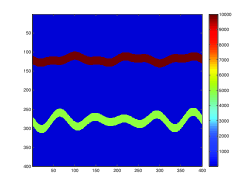
Figure 1: Samples of permeability field used in numerical examples

Next, we present the details of numerical discretization of the problem. Suppose the spatial domain $\Omega$ is partitioned into a rectangular mesh $\mathcal{T}_{h}$, and a set of piecewise bilinear conforming finite element basis functions $\{v_{j}\}$ is constructed on the mesh. We denote the finite element space by $V_{h}=\mathbb{Q}^{1}(\mathcal{T}_{h})$. Using a direct linearization method for the nonlinearity term, implicit Euler method for temporal discretization and a Galerkin finite element method for spatial discretization, the numerical solution $u_{h}^{n+1}$ at the time instant $n+1$ is obtained by solving the following variational formulation: find $u_{h}^{n+1}\in V_{h}$ such that

$$\int_{\Omega}\frac{u_{h}^{n+1}-u_{h}^{n}}{\Delta t}v+\int_{\Omega}\kappa\exp(\alpha u_{h}^{n})\nabla u_{h}^{n+1}\cdot\nabla v=\int_{\Omega}g^{n+1}v\quad\text{ for all }v\in V_{h}.$$ (3)

Here $\Delta t$ is the time step and $h$ is the mesh size. With a slight abuse of notation, we again denote the coefficients of the numerical solution with the piecewise bilinear basis functions by $u_{h}^{n+1}$. Then, the variational formulation can be written in the matrix form

$$u_{h}^{n+1}=(M+\Delta tA^{n+1})^{-1}Mu_{h}^{n}+\Delta tb^{n+1},$$ (4)

where $M$, $A^{n+1}$ and $b^{n+1}$ are the mass matrix, the stiffness matrix and the load vector with respect to the bilinear basis functions functions $v_{j}$, i.e.,

$$\begin{split}M_{ij}&=\int_{\Omega}v_{i}v_{j},\\ A^{n+1}_{ij}&=\int_{\Omega}\kappa\exp(\alpha u_{h}^{n})\nabla v_{i}\cdot\nabla v_{j},\\ b^{n+1}_{i}&=\int_{\Omega}g^{n+1}v_{i}.\end{split}$$ (5)

2.1 Model order reduction by Proper Orthogonal Decomposition

Proper Orthogonal Decomposition is a popular mode decomposition method, which aims at reducing the order of the model by extracting important relevant feature representation with a low dimensional space. In this section, we briefly discuss the POD method on our model problem (3). For a more detailed discussion of the use of POD on dynamic systems, the reader is referred to [19, 22]. In POD, a low-dimensional set of modes, i.e., important degrees of freedom, are identified based on processing information from a sequence of snapshots, i.e., instantaneous solutions from the dynamic process, and extracting the most energetic structures in terms of the largest singular values. In the statistical point of view, the extracted modes are uncorrelated and form an optimal reduced order model, in the sense that the variance is maximized and the mean squared distance between the snapshots and the POD subspace is minimized. The POD subspace is then used to derive a reduced-order dynamical system by a Galerkin projection.

Proper orthogonal decomposition starts with a collection of $N$ instantaneous snapshots

$$\Phi=[\phi_{1}\;\;\phi_{2}\;\;\cdots\;\;\phi_{N}],$$

where the snapshot times in the above sequence is assumed to be equidistant. POD is then processed by performing a singular value decomposition on $\Phi$. We denote the correlation matrix from the snapshot sequence by $C=\Phi^{T}\Phi$, and compute the eigenvalue decomposition on $C$ to obtain the POD modes $\xi_{j}$ by

$$Cw_{j}=\sigma_{j}^{2}w_{j}\text{ and }\xi_{j}=\dfrac{1}{\sigma_{j}}\Phi w_{j}.$$

Here, $\sigma_{j}$ and $\xi_{j}$ are referred to the singular values and left-singular vectors of $\Phi$. The singular values, which correspond to the energy content of a mode, provide a measure of the importance of the mode in capturing the relevant dynamic process. The POD subspace is obtained by selecting the first few POD modes in descending energy ranking, i.e., we arrange the POD modes by $\sigma_{1}\geq\sigma_{2}\geq\cdots\geq\sigma_{N}$ and take the first few modes $\{\xi_{j}\}_{j=1}^{m}$ as a basis for the POD subspace $W_{h}\subset V_{h}$. The reduced-order model for (3) is then given by a Galerkin projection: find $\widetilde{u}_{h}^{n+1}\in W_{h}$ such that

$$\int_{\Omega}\frac{\widetilde{u}_{h}^{n+1}-\widetilde{u}_{h}^{n}}{\Delta t}v+\int_{\Omega}\kappa\exp(\alpha\widetilde{u}_{h}^{n})\nabla\widetilde{u}_{h}^{n+1}\cdot\nabla v=\int_{\Omega}g^{n+1}v\quad\text{ for all }v\in W_{h}.$$ (6)

2.2 Construction of nodal basis functions

Next, we present the construction of our POD basis functions. The basis functions are designed such that the degrees of freedom have physical meanings (e.g., represent the solution values at selected locations). Since the constructed basis functions have limited support, it will allow localizing the forward dynamics by writing the forward map for the solution values at selected locations with pre-computed neighborhood structure.

Given a set of nodes $\{x_{k}\}_{k=1}^{m}$ in the mesh $\mathcal{T}_{h}$, which correspond to particular points in the physical domain $\Omega$, we construct nodal basis functions by linear combinations of POD modes $\{\xi_{j}\}_{j=1}^{m}$. More precisely, we seek coefficients $\alpha_{ij}$ such that

$$\sum_{j=1}^{m}\alpha_{ij}\xi_{j}(x_{k})=\delta_{ik}.$$

The nodal basis function $\psi_{k}$ is then defined by

$$\psi_{k}=\sum_{j=1}^{m}\alpha_{kj}\xi_{j}.$$

Examples of nodal basis functions are shown in Figure 2. A numerical approximation $\widetilde{u}_{h}^{n}$ in the POD subspace $W_{h}$ can then be written in the expansion

$$\widetilde{u}_{h}^{n}=\sum_{k=1}^{m}c_{k}^{n}\psi_{k},$$

where the coefficients $c_{k}^{n}=u_{h}^{n}(x_{k})$ denote the evaluation of $u_{h}^{n}$ at the node $x_{k}$. We align the coordinate representation of the nodal basis functions column by column and form a matrix

$$\Psi=[\psi_{1}\;\;\psi_{2}\;\;\cdots\;\;\psi_{m}].$$

The Galerkin projection reduced-order model (6) can then be written in a matrix form:

$$c^{n+1}=(\widetilde{M}+\Delta t\widetilde{A}^{n+1})^{-1}\widetilde{M}c^{n}+\Delta t\widetilde{b}^{n+1},$$ (7)

where $\widetilde{M}$, $\widetilde{A}^{n+1}$ and $\widetilde{b}^{n+1}$ are the mass matrix, the stiffness matrix and the load vector with respect to the POD nodal basis functions $\psi_{j}$, i.e.,

$$\begin{split}\widetilde{M}&=\Psi^{T}M\Psi,\\ \widetilde{A}^{n+1}&=\Psi^{T}A^{n+1}\Psi,\\ \widetilde{b}^{n+1}&=\Psi^{T}b^{n+1}.\end{split}$$ (8)

We remark that in (7), the coefficients in a time instant $n+1$, $c^{n+1}$, is nonlinearly dependent on the the coefficients in the previous time instant $c^{n}$, and input parameters such as the permeability field $\kappa$ and source function $g^{n+1}$.

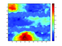
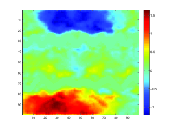
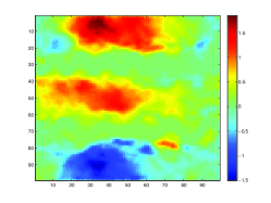
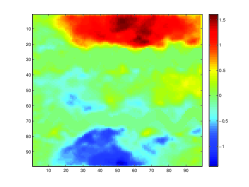
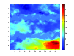
Figure 2: Illustration of nodal basis functions.

3 Deep Global Model Reduction and Learning

3.1 Main idea

We will make use of the reduced-order model described in Section 2 to model the flow dynamics, and a deep neural network to approximate the flow profile. In many cases, the flow profile is dependent on data. The idea of this work is to make use of deep learning to combine the reduced-order model and available data and provide an efficient numerical model for modelling the flow profile.

First, we note that the solution at the time instant $n+1$ depends on the solution at the time instant $n$ and input parameters $I^{n+1}$, such as permeability field and source terms. Here, we would like to use a neural network to describe the relationship of the solutions between two consecutive time instants. Suppose we have a total $m$ sample realization in the training set. For each realization, given a set of input parameters, we solve the aforementioned reduced-order model and obtain the nodal values at particular points

$$\{c^{0},\cdots,c^{k}\}$$

at all time steps. Our goal is to use deep learning techniques to train the trajectories and find a network $\mathcal{N}$ to describe the pushforward map between $c^{n}$ and $c^{n+1}$ for any training sample.

$$c^{n+1}\sim\mathcal{N}(c^{n},I^{n+1}),$$

where $I^{n+1}$ is an input parameter which could vary over time, and $\mathcal{N}$ is a multi-layer network to be trained. The network $\mathcal{N}$ will approximate the discrete flow dynamics (7).

In our neural network, $c^{n}$ and $I^{n+1}$ are the inputs, $c^{n+1}$ is the output. One can take the nodal values from time $0$ to time $k-1$ as input, and from time $1$ to $k$ as output in the training process. In this case, a universal neural net $\mathcal{N}$ is obtained. The solution at time $0$ can then be forwarded all the way to time $k$ by repeatedly applying the universal network $k$ times, that is,

$$c^{k}\sim\mathcal{N}(\mathcal{N}\cdots\mathcal{N}(c^{0},I^{1})\cdots,I^{k-1}),I^{k}).$$

After a network is trained, it can be used for predicting the trajectory given a new set of input parameters $I^{n+1}$ and realization of nodal value at initial time $c_{\text{new}}^{0}$ by

$$c_{\text{new}}^{k}\sim\mathcal{N}(\mathcal{N}\cdots\mathcal{N}(c_{\text{new}}^{0},I^{1})\cdots,I^{k-1}),I^{k}).$$

Alternatively, one can also train each forward map for any two consecutive time instants as needed. That is, we will have $c^{n+1}\sim\mathcal{N}_{n+1}(c^{n},I^{n+1})$, for $n=0,1,\ldots,k-1$. In this case, to predict the final time solution ${c_{\text{new}}^{k}}$ given the initial time solution ${c_{\text{new}}}^{0}$, we use $k$ different networks $\mathcal{N}_{1},\cdots,\mathcal{N}_{k}$

$$c_{\text{new}}^{k}\sim\mathcal{N}_{k}(\mathcal{N}_{k-1}\cdots\mathcal{N}_{1}(c_{\text{new}}^{0},I^{1})\cdots,I^{k-1}),I^{k}).$$

We remark that, besides the solution $u^{n}$ at the previous time instant, the other input parameters $I^{n+1}$ such as permeability or source terms can be different when entering the network at different time steps.

In this work, we would like to incorporate available observed data in the neural network. The observation data will help to supplement the computational data which are obtained from the underlying reduced order model, and improve the performance of the neural network model such that it will take into account real data effects. From now on, we use $\{c_{s}^{0},\cdots,c_{s}^{k}\}$ to denote the simulation data, and $\{c_{o}^{0},\cdots,c_{o}^{k}\}$ to denote the observation data.

One can get the observation data from real field experiment. However in this work, we generate the observation data by running a new simulation on the “true permeability field” using standard finite element method, and using the results as observed data. For the computational data, we will perturb the “true permeability field”, and use the reduced-order model, i.e., POD model for simulation. In the training process, we are interested in investigating the effects of observation data in the output. One can compare the performance of deep neural networks when using different combinations of computation and observation data.

For the comparison, we will consider the following three networks

• Network A: Use all observation data as output,

  $${c_{o}}^{n+1}\sim\mathcal{N}_{o}({c_{s}}^{n},I^{n+1})$$ (9)

• Network B: Use a mixture of observation data and simulation data as output,

  $${c_{m}}^{n+1}\sim\mathcal{N}_{m}({c_{s}}^{n},I^{n+1})$$ (10)

• Network C: Use all simulation data (no observation data) as output,

  $${c_{s}}^{n+1}\sim\mathcal{N}_{s}({c_{s}}^{n},I^{n+1})$$ (11)

where $c_{m}$ is a mixture of simulation data and observed data.

The first network (Network A) corresponds to the case when the observation data is sufficient. One can merely utilize the observation data in the training process. That is, the observation data at time $n+1$ can be learnt as a function of the observation data at time $n$. This map will fit the real data very well given enough training data; however, it will not be able to approximate the reduced-order model. Moreover, in the real application, the observation data are hard to obtain, and in order to make the training effective, deep learning requires a huge amount of data. Thus Network A is not applicable in real case, and we will use the results from Network A as a reference.

The third network (Network C), on the other hand, will simply take all simulation data in the training process. In this case, one will get a network describes the simulation model (in our example, the POD reduced-order model) as best as it can but ignore the observational data effects. This network can serve as an emulator to do a fast simulation. We will also utilize Network C results as a reference.

We are interested in investigating the performance of Network B, where we take a combination of computational data and observational data to train. It will not only take in to account the underlying physics but also use the real data to modify the reduced-order model, thus resulting in a data-driven model.

3.2 Network structures

Mathematically, a neural network $\mathcal{N}$ of $L$ layers with input $\mathbf{x}$ and output $\mathbf{y}$ is a function in the form

$$\mathcal{N}(\mathbf{x};\theta)=\sigma(W_{L}\sigma(\cdots\sigma(W_{2}\sigma(W_{1}\mathbf{x}+b_{1})+b_{2})\cdots)+b_{L})$$

where $\theta:=(W_{1},\cdots,W_{L},b_{1},\cdots,b_{L})$ is a set of network parameters, $W$’s are the weight matrices and $b$’s are the bias vectors. The activation function $\sigma$ acts as entry-wise evaluation. A neural network describes the connection of a collection of nodes (neurons) sit in successive layers. The output neurons in each layer is simultaneously the input neurons in the next layer. The data propagate from the input layer to the output layer through hidden layers. The neurons can be switched on or off as the input is propagated forward through the network. The weight matrices $W$’s control the connectivity of the neurons. The number of layers $L$ describes the depth of the neural network. Figure 3 depicts a deep neural network in out setting, in which each circular node represents a neuron and each line represents a connection from one neuron to another. The input layer of the neural network consists of the coefficients $c^{n}$ and the input parameters $I^{n}$.

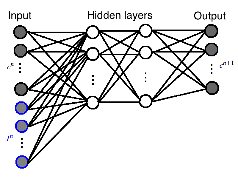
Figure 3: An illustration of deep neural network

Given a set of data $(\mathbf{x}_{j},\mathbf{y}_{j})$, the deep neural network aims to find the parameters $\theta^{*}$ by solving an optimization problem

$$\theta^{*}=\operatorname*{\text{argmin}}_{\theta}\frac{1}{N}\sum_{j=1}^{N}||\mathbf{y}_{j}-\mathcal{N}(\mathbf{x}_{j};\theta)||^{2}_{2},$$

where $N$ is the number of the samples. Here, the function $\frac{1}{N}\sum_{j=1}^{N}||\mathbf{y}_{j}-\mathcal{N}(\mathbf{x}_{j};\theta)||^{2}_{2}$ is known as the loss function. One needs to select suitable number of layers, number of neurons in each layer, the activation function, the loss function and the optimizers for the network.

As discussed in the previous section, we consider three different networks, namely $\mathcal{N}_{o}$, $\mathcal{N}_{m}$ and $\mathcal{N}_{s}$. For each of these networks, we take the vector $\mathbf{x}=({c_{s}}^{n},I^{n+1})$ containing the numerical solution vectors and the data at a particular time step as the input. In our setting, the input parameter $I^{n+1}$, if present, could be the static permeability field or the source function. Based on the availability of the observational data in the sample pairs, we will select an appropriate network among (9), (10) and (11) accordingly. The output $\mathbf{y}={c_{\alpha}}^{n+1}$ is taken as the numerical solution at the next time instant, where $\alpha=o,m,s$ corresponds to the network.

Here, we briefly summarize the architecture of the network $\mathcal{N}_{\alpha}$, where $\alpha=o,m,s$ for three networks we defined in (9), (10) and (11) respectively.

As for the input of the network, we use $\mathbf{x}=({c_{s}}^{n},I^{n+1})$, which are the vectors containing the numerical solution vectors and the input parameters in a particular time step. The corresponding output data are $\mathbf{y}={c_{\alpha}}^{n+1}$, which contains the numerical solution in the next time step. In between the input and output layer, we test on 3–10 hidden layers with 20-400 neurons in each hidden layer. In the training, there are $N=mk$ sample pairs of $(\mathbf{x}_{j},\mathbf{y}_{j})$ collected, where $m$ is the number of realizations of flow dynamics and $k$ is the number of time steps.

In between layers, we need the activation function. The ReLU function (rectified linear unit activation function) is a popular choice for activation function in training deep neural network architectures [16]. However, in optimizing a neural network with ReLU as activation function, weights on neurons which do not activate initially will not be adjusted, resulting in slow convergence. Alternatively, leaky ReLU can be employed to avoid such scenarios [27]. We choose leaky ReLU in our network structure.

Another important ingredients in the deep neural network is choosing appropriate loss functions. Here we consider two types of loss functions.

• Standard loss function: $\frac{1}{N}\sum_{j=1}^{N}\|\mathbf{y}_{j}-\mathcal{N}_{\alpha}(\mathbf{x}_{j};\theta)\|_{2}^{2}$.

• Weighted loss function: In building a network in $\mathcal{N}_{m}$ by using a mixture of $N_{1}$ pairs of observation data $\{(\mathbf{x}_{j},\mathbf{y}_{j})\}_{j=1}^{N_{1}}$ and $N_{2}$ pairs of observation data $\{(\mathbf{x}_{j},\mathbf{y}_{j})\}_{j=N_{1}+1}^{N}$, where $N_{1}+N_{2}=N$, we may consider using weighted loss function, i.e, $w_{1}\sum_{j=1}^{N_{1}}\|\mathbf{y}_{j}-\mathcal{N}_{m}(\mathbf{x}_{j};\theta)\|_{2}^{2}+w_{2}\sum_{j=N_{1}+1}^{N}\|\mathbf{y}_{j}-\mathcal{N}_{m}(\mathbf{x}_{j};\theta)\|_{2}^{2}$, where $w_{1}>w_{2}$ are user-defined weights.

As for the training optimizer, we use AdaMax [24], which is a stochastic gradient descent (SGD) type algorithm well-suited for high-dimensional parameter space, in minimizing the loss function.

Remark 1.

We note that the discretization parameters (see (8)) can be learned using proposed DL techniques. Our numerical results show that one can achieve a very good accuracy (about 2 %) using DNN with 5 layers and 100 neurons in each layer. These results show that deep learning techniques can be used for fast prediction of discretized systems. In our paper, our main goal was to incorporate the observed data into the dynamical system and modify reduced-order models to take into account the observed data. We have also used deep learning techniques to predict online basis functions [12, 1, 6], which allow re-constructing the fine-scale solution.

4 Numerical examples

In this section, we present numerical examples. In all experiments, the nonlinear constant is set to be $\alpha=20$, and the time-step is $\Delta t=0.1$. We consider the flow dynamics from an initial time $t=0$ to a final time $t=1$ in $10$ time steps. In each experiment, a POD subspace is precomputed and used as a reduced-order model. Simulation data of the dynamic process under the reduced-order model are then obtained and used in the training set. In some cases, observation data are supplemented in the training set. Different forms of inputs, depending on situations, are investigated. Using these data as samples, universal multi-layer networks are trained to approximate the flow dynamic. We use the trained networks to predict the flow dynamics with some new experimental inputs. We examine the quality of our networks by computing the $L^{2}$ error between our predicted solution $\widetilde{u}_{\text{pred}}^{n}$ and some reference solution $u_{\text{ref}}^{n}$, i.e.,

$$\|u_{\text{ref}}^{n}-u_{\text{pred}}^{n}\|_{L^{2}(\Omega)}=\left(\int_{\Omega}|u_{\text{ref}}^{n}-u_{\text{pred}}^{n}|^{2}\,dx\right)^{\frac{1}{2}}.$$

All the network training are performed using the Python deep learning API Keras [5].

4.1 Experiment 1

In this experiment, we consider a flow dynamic problem with the static coefficient field $\kappa$ and a time-independent source $g$ fixed among all the samples. In the neural network, we simply take the input and output as

$$\mathbf{x}={c_{s}}^{n}\quad\text{ and }\quad\mathbf{y}={c_{s}}^{n+1}.$$

In the generation of samples, we consider independent and uniformly distributed initial conditions ${c_{s}}^{0}$. We generate $100$ realizations of initial conditions ${c_{s}}^{0}$, and evolve the reduced-order dynamic process to obtain ${c_{s}}^{n}$ for $n=1,2,\ldots,10$ . We remark that these simulation data provide a total of $1000$ samples of the pushforward map.

We use the $900$ samples given by $90$ realizations as training set and the $100$ samples given by $10$ remaining realizations as testing samples. Using the training data and a given network architecture, we find a set of optimized parameter $\theta^{*}$ which minimizes the loss function, and obtain an optimized network $\mathcal{N}_{\theta^{*}}$. The network $\mathcal{N}_{\theta^{*}}$ is then used to predict the $1$-step dynamic, i.e.,

$${c_{s}}^{n+1}\approx\mathcal{N}_{\theta^{*}}({c_{s}}^{n}).$$

We also use the composition of the network $\mathcal{N}_{\theta^{*}}$ to predict the final-time solution, i.e.,

$${c_{s}}^{10}\approx\mathcal{N}_{\theta^{*}}(\mathcal{N}_{\theta^{*}}(\cdots\mathcal{N}_{\theta^{*}}({c_{s}}^{0})\cdots)).$$

We use the same set of training data and testing data and compare the performance of different network architectures. We examine the performance of the networks by the mean of $L^{2}$ percentage error of the $1$-step prediction and the final-time prediction in the testing samples. The error is computed by comparing to the solution formed by the simulation data ${c_{s}}^{n}$. The results are summarized in Table 1. It can be observed that with a more complex network architecture, i.e., more layers and neurons, the quality of the prediction tends to be better. Figure 4 depicts the reference solutions and the predicted solutions at final time with different inputs. The figure shows that the predicted solution is in a good agreement with the reference solution.

Layer	Neuron	$1$-step	Final-time
3	20	0.1776	3.4501e+09
	100	0.0798	6.3276
	400	0.0613	4.9855
5	20	0.1499	6.5970e+06
	100	0.0753	6.3101
	400	0.0602	4.8137
10	20	0.1024	5.4183
	100	0.0750	4.3271
	400	0.0609	1.8834

Table 1: Mean of $L^{2}$ percentage error with different network architectures in Experiment 1

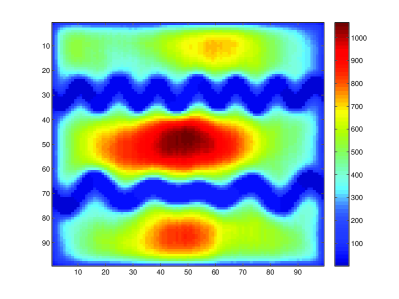
Figure 4: Plots of reference solution (left) and predicted solution (right) at final time in Experiment 1

4.2 Experiment 2

In this experiment, we consider a flow dynamic problem with a time-independent source $g$ fixed among all the samples, while the static permeability field $\kappa$ is varying among the samples. In the neural network, we take the input and output as

$$\mathbf{x}=({c_{s}}^{n},\kappa)\quad\text{ and }\quad\mathbf{y}={c_{s}}^{n+1}.$$

In the generation of samples, we consider independent and uniformly distributed initial conditions ${c_{s}}^{0}$. We pick $10$ different configurations of the permeability field $\kappa$, generate $10$ realizations of initial conditions ${c_{s}}^{0}$ for each configuration, and evolve the reduced-order dynamic process to obtain ${c_{s}}^{n}$ for $n=1,2,\ldots,10$ . We remark that these simulation data provide a total of $1000$ samples of the pushforward map.

We use the $900$ samples given by $90$ realizations as training set and the $100$ samples given by $10$ remaining realizations as testing samples. Using the training data and a given network architecture, we find a set of optimized parameter $\theta^{*}$ which minimizes the loss function, and obtain an optimized network $\mathcal{N}_{\theta^{*}}$. The network $\mathcal{N}_{\theta^{*}}$ is then used to predict the $1$-step dynamic, i.e.,

$${c_{s}}^{n+1}\approx\mathcal{N}_{\theta^{*}}({c_{s}}^{n},\kappa).$$

We also use the composition of the network $\mathcal{N}_{\theta^{*}}$ to predict the final-time solution, i.e.,

$${c_{s}}^{10}\approx\mathcal{N}_{\theta^{*}}(\mathcal{N}_{\theta^{*}}(\cdots\mathcal{N}_{\theta^{*}}({c_{s}}^{0},\kappa)\cdots,\kappa),\kappa).$$

We use the same set of training data and testing data and compare the performance of different number of layers. We examine the performance of the networks by the mean of $L^{2}$ percentage error of the $1$-step prediction and the final-time prediction in the testing samples. The error is computed by comparing to the solution formed by the simulation data ${c_{s}}^{n}$. The results are summarized in Tables 2 and 3. In Table 2, there are $9$ out of $10$ realizations in the training set for each configuration of the static field $\kappa$. The results show that the error is reasonable. Again, it can be observed that with more layers in the neural network, the quality of the prediction tends to be better. In Table 3, the training set consists of all realizations of $9$ configurations among $10$, and the samples of the remaining configuration are used for testing. In this case, there are no common input, i.e., configurations, in the training set and the learning set. It can be seen that the prediction is bad, even with a deep neural network. This shows that data with similar input is essential in building a useful network. Figure 5 depicts the reference solutions and the predicted solutions at final time with different inputs. Again, the figure shows that the predicted solution is in a good agreement with the reference solution. Moreover, it can be seen that with the same network, the predicted solutions successfully capture the channel configuration. This shows that the trained network correctly addresses the permeability field $\kappa$ as an input to the predicted solution as an output as desired.

Layer	$1$-step	Final-time
2	7.4647	19.8207
3	6.8709	8.3702
4	6.5983	9.5155
5	7.2846	5.0525
10	7.5914	4.0498

Table 2: Mean of $L^{2}$ percentage error with common configuration in training and learning set in Experiment 2.

Layer	$1$-step	Final-time
2	72.5023	6.3525e+03
3	84.7095	8.5841e+03
4	129.7150	1.2905e+04
5	109.9931	7.4646e+03
10	584.4894	6.5055e+04

Table 3: Mean of $L^{2}$ percentage error without common configuration in training and learning set in Experiment 2.

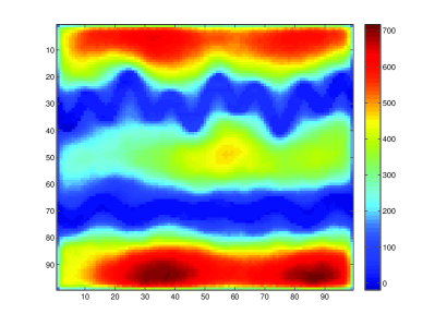
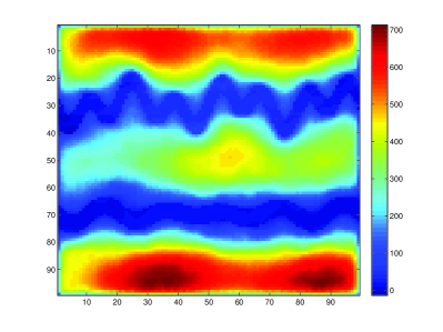
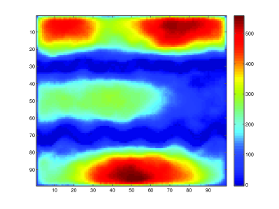
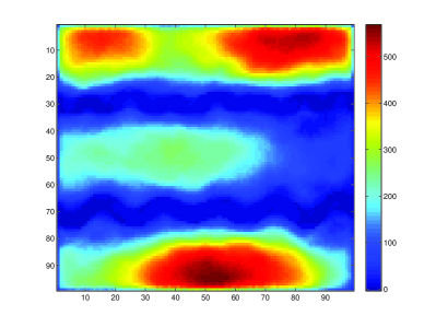
Figure 5: Plots of reference solutions (left) and predicted solutions (right) at final time of $2$ realizations in Experiment 2

4.3 Experiment 3

In this experiment, we consider a flow dynamic problem with a time-dependent source $g$ fixed among all the samples, and the static permeability field $\kappa$ is varying among the samples. In the neural network, we take the input and output as

$$\mathbf{x}=({c_{s}}^{n},\kappa,g^{n+1})\quad\text{ and }\quad\mathbf{y}={c_{s}}^{n+1}.$$

In the generation of samples, we consider independent and uniformly distributed initial conditions ${c_{s}}^{0}$. We pick $10$ different configurations of the permeability field $\kappa$, generate $10$ realizations of initial conditions ${c_{s}}^{0}$ for each configuration, and evolve the reduced-order dynamic process to obtain ${c_{s}}^{n}$ for $n=1,2,\ldots,10$ . We remark that these simulation data provide a total of $1000$ samples of the pushforward map.

We use the $900$ samples given by $90$ realizations as training set and the $100$ samples given by $10$ remaining realizations as testing samples. Using the training data and a given network architecture, we find a set of optimized parameter $\theta^{*}$ which minimizes the loss function, and obtain an optimized network $\mathcal{N}_{\theta^{*}}$. The network $\mathcal{N}_{\theta^{*}}$ is then used to predict the $1$-step dynamic, i.e.,

$${c_{s}}^{n+1}\approx\mathcal{N}_{\theta^{*}}({c_{s}}^{n},\kappa,g^{n+1}).$$

We also use the composition of the network $\mathcal{N}_{\theta^{*}}$ to predict the final-time solution, i.e.,

$${c_{s}}^{10}\approx\mathcal{N}_{\theta^{*}}(\mathcal{N}_{\theta^{*}}(\cdots\mathcal{N}_{\theta^{*}}({c_{s}}^{0},\kappa,g^{1})\cdots,\kappa,g^{9}),\kappa,g^{10}).$$

We use the same set of training data and testing data and compare the performance of different number of layers. We examine the performance of the networks by the mean of $L^{2}$ percentage error of the $1$-step prediction and the final-time prediction in the testing samples. The error is computed by comparing to the solution formed by the simulation data ${c_{s}}^{n}$. The results are summarized in Table 4. It can be observed that with a deep neural network, the quality of the prediction tends to be better.

Layer	$1$-step	Final-time
2	5.6382	1.8997e+07
3	3.6035	4.5991
4	2.9029	1.5968
5	2.4335	1.4755
10	2.5834	0.2595

Table 4: Mean of $L^{2}$ percentage error in Experiment 3.

4.4 Experiment 4

In this experiment, we consider a flow dynamic problem with the static permeability field $\kappa$ and the time-dependent source $g$ varying among the samples. In the neural network, we take the input and output as

$$\mathbf{x}=({c_{s}}^{n},\kappa,g^{n+1})\quad\text{ and }\quad\mathbf{y}={c_{\alpha}}^{n+1}.$$

We compare the performance of different networks in (9)–(11), using different numbers and types of sample points in the training set. More specifically, we generate two set of samples, namely observation samples and simulation samples. In the generation of observation samples, we fix a configuration for the static field $\kappa_{o}$ and obtain a slightly perturbed configuration $\kappa_{s}$ from the static field $\kappa_{o}$. The permeability fields used are illustrated in Figure 6.

Figure 6: Permeability fields $\kappa_{o}$ (left) for observation data and $\kappa_{s}$ (right) for simulation data respectively.

To compare the networks, we take observation data using the field $\kappa_{o}$, and generate simulation data using the reduced-order model with the field $\kappa_{s}$. For both kinds of data, we consider independent and uniformly distributed initial conditions ${c_{s}}^{0}$ with equal occurrence probability. We start with $100$ realizations of initial conditions ${c_{s}}^{0}$, and obtain ${c_{\alpha}}^{n}$ for $n=1,2,\ldots,10$ accordingly. We remark that either observation data and simulation data provides a total of $1000$ samples of the pushforward map.

Using these samples, we train networks using the following samples in the training set:

• Case 1: $\mathcal{N}_{s}$ with 100 realizations from simulation data,

• Case 2: $\mathcal{N}_{m}$ with 90 realizations from simulation data and 10 realizations from observation data,

• Case 3: $\mathcal{N}_{o}$ with 100 realizations from observation data, and

• Case 4: $\mathcal{N}_{o}$ with 10 realizations from observation data only.

We additionally take $10$ observation realizations in testing the optimized network $\mathcal{N}_{\theta^{*}}$. We use the composition of the network $\mathcal{N}_{\theta^{*}}$ to predict the final-time solution, i.e.,

$${c_{\alpha}}^{10}\approx\mathcal{N}_{\theta^{*}}(\mathcal{N}_{\theta^{*}}(\cdots\mathcal{N}_{\theta^{*}}({c_{s}}^{0},\kappa,g^{1}),\cdots,\kappa,g^{9}),\kappa,g^{10}).$$

We use the same network architecture and compare the networks using different sets of training data and testing data. We examine the performance of the networks by the mean of $L^{2}$ percentage error of the $1$-step prediction and the final-time prediction in the testing samples. The error is computed by comparing to the solution formed by the observation data ${c_{o}}^{n}$. The results are summarized in Tables 5. By comparing cases 1–3, we see that the network with $100$ realizations from observation performs better than the other networks with the same number of realizations. Moreover, by comparing cases 3 and 4, we observe that if the number of observation samples is reduced, the performance becomes worse. However, if we supplement the observation data with simulation data, the results is improved as in case 2. This shows that the data-driven approach is useful in taking observation data into account, and simulation data can help improving the network in the deficiency of insufficient observation data. Using observed data, we can modify the forward reduced-order model that can take into account the data.

Case	Final-time
1	31.1781
2	16.6937
3	15.9991
4	21.8747

Table 5: $L^{2}$ percentage error in final time in Experiment 4

5 Conclusion

In this paper, we combine some POD techniques with deep learning concepts in the simulations for flows in porous media. The observation data is given at some (well) locations. We construct POD modes such that the degrees of freedom represent the values of the solution at well locations. Furthermore, we write the solution at the current time as a multi-layer network that depends on the solution at the initial time and input parameters, such as well rates and permeability fields. This provides a natural framework for applying deep learning techniques for flows in channelized media. We provide the details of our method and present numerical results. In all numerical results, we study nonlinear flow equation in channelized media and consider various channel configurations. Our results show that multi-layer network provides an accurate approximation of the forward map and can incorporate the observed data. Moreover, by incorporating some observed data (from true model) and some computational data, we modify the reduced-order model. This way, one can use the observed data to modify reduced-order models which honor the observed data.

References

- [1] Manal Alotaibi, Victor M. Calo, Yalchin Efendiev, Juan Galvis, and Mehdi Ghommem. Global-local nonlinear model reduction for flows in heterogeneous porous media. Computer Methods in Applied Mechanics and Engineering, 292:122–137, 2015.
- [2] M. Cardoso and L. Durlofsky. Linearized reduced-order models for subsurface flow simulation. Journal of Computational Physics, 229, 2010.
- [3] MA Cardoso, LJ Durlofsky, and P Sarma. Development and application of reduced-order modeling procedures for subsurface flow simulation. International journal for numerical methods in engineering, 77(9):1322–1350, 2009.
- [4] Michael A Celia, Efthimios T Bouloutas, and Rebecca L Zarba. A general mass-conservative numerical solution for the unsaturated flow equation. Water resources research, 26(7):1483–1496, 1990.
- [5] François Chollet et al. Keras. https://keras.io, 2015.
- [6] E. T. Chung, Y. Efendiev, and W. T. Leung. Residual-driven online generalized multiscale finite element methods. Journal of Computational Physics, 302:176–190, 2015.
- [7] Balázs Csanád Csáji. Approximation with artificial neural networks. Faculty of Sciences, Etvs Lornd University, 24(48), 2001.
- [8] G. Cybenko. Approximations by superpositions of sigmoidal functions. Mathematics of Control, Signals, and Systems, 2(4):303–314, 1989.
- [9] P Dostert, Y Efendiev, and B Mohanty. Efficient uncertainty quantification techniques in inverse problems for richards’ equation using coarse-scale simulation models. Advances in water resources, 32(3):329–339, 2009.
- [10] Y Efendiev, A Datta-Gupta, V Ginting, X Ma, and B Mallick. An efficient two-stage markov chain monte carlo method for dynamic data integration. Water Resources Research, 41(12), 2005.
- [11] Yalchin Efendiev, Juan Galvis, and Eduardo Gildin. Local–global multiscale model reduction for flows in high-contrast heterogeneous media. Journal of Computational Physics, 231(24):8100–8113, 2012.
- [12] Yalchin Efendiev, Eduardo Gildin, and Yanfang Yang. Online adaptive local-global model reduction for flows in heterogeneous porous media. Computation, 4(2):22, 2016.
- [13] WR Gardner. Some steady-state solutions of the unsaturated moisture flow equation with application to evaporation from a water table. Soil science, 85(4):228–232, 1958.
- [14] Mehdi Ghommem, Victor M. Calo, and Yalchin Efendiev. Mode decomposition methods for flows in high-contrast porous media. a global approach. Journal of Computational Physics, 257:400–413, 2014.
- [15] Mehdi Ghommem, Michael Presho, Victor M. Calo, and Yalchin Efendiev. Mode decomposition methods for flows in high-contrast porous media. global-local approach. Journal of Computational Physics, 253:226–238, 2013.
- [16] Xavier Glorot, Antoine Bordes, and Yoshua Bengio. Deep sparse rectifier neural networks. In Proceedings of the Fourteenth International Conference on Artificial Intelligence and Statistics, pages 315–323. PMLR, 2011.
- [17] Ian Goodfellow, Yoshua Bengio, Aaron Courville, and Yoshua Bengio. Deep learning, volume 1. MIT press Cambridge, 2016.
- [18] Boris Hanin. Universal function approximation by deep neural nets with bounded width and relu activations. arXiv:1708.02691, 2017.
- [19] M. Hinze and S. Volkwein. Proper orthogonal decomposition surrogate models for nonlinear dynamical systems: error estimates and suboptimal control. In P. Benner, V. Mehrmann, and D.C. Sorensen, editors, Dimension Reduction of Large-Scale Systems, volume 45 of Lecture Notes in Computational Science and Engineering, pages 261–306. Springer Berlin Heidelberg, 2005.
- [20] Kurt Hornik. Approximation capabilities of multilayer feedforward networks. Neural Networks, 4(2):251–257, 1991.
- [21] Jan Dirk Jansen and Louis J Durlofsky. Use of reduced-order models in well control optimization. Optimization and Engineering, 18(1):105–132, 2017.
- [22] Gaetan Kerschen, Jean-claude Golinval, Alexander F. Vakakis, and Lawrence A. Bergman. The method of proper orthogonal decomposition for dynamical characterization and order reduction of mechanical systems: An overview. Nonlinear Dynamics, 41(1):147–169, 2005.
- [23] Yuehaw Khoo, Jianfeng Lu, and Lexing Ying. Solving parametric pde problems with artificial neural networks. arXiv:1707.03351, 2017.
- [24] Diederik P. Kingma and Jimmy Ba. Adam: A method for stochastic optimization. arXiv preprint arXiv:1412.6980, 2014.
- [25] Yann LeCun, Yoshua Bengio, and Geoffrey Hinton. Deep learning. nature, 521(7553):436, 2015.
- [26] Zhen Li and Zuoqiang Shi. Deep residual learning and pdes on manifold. arXiv:1708.05115., 2017.
- [27] A.L. Maas, A.Y. Hannun, and A.Y. Ng. Rectifier nonlinearities improve neural network acoustic models. Proc. icml, 30(1), 2013.
- [28] H. Mhaskar Q. Liao and T. Poggio. Learning functions: when is deep better than shallow. arXiv:1603.00988v4, 2016.
- [29] Lorenzo Adolph Richards. Capillary conduction of liquids through porous mediums. physics, 1(5):318–333, 1931.
- [30] Jürgen Schmidhuber. Deep learning in neural networks: An overview. Neural networks, 61:85–117, 2015.
- [31] M. Telgrasky. Benefits of depth in neural nets. JMLR: Workshop and Conference Proceedings, 49(123), 2016.
- [32] Sumeet Trehan and Louis J Durlofsky. Trajectory piecewise quadratic reduced-order model for subsurface flow, with application to pde-constrained optimization. Journal of Computational Physics, 326:446–473, 2016.
- [33] Jorn FM van Doren, Renato Markovinović, and Jan-Dirk Jansen. Reduced-order optimal control of water flooding using proper orthogonal decomposition. Computational Geosciences, 10(1):137–158, 2006.
- [34] M Th Van Genuchten. A closed-form equation for predicting the hydraulic conductivity of unsaturated soils 1. Soil science society of America journal, 44(5):892–898, 1980.
- [35] Hai X Vo and Louis J Durlofsky. A new differentiable parameterization based on principal component analysis for the low-dimensional representation of complex geological models. Mathematical Geosciences, 46(7):775–813, 2014.
- [36] E. Weinan and Bing Yu. The deep Ritz method: A deep learning-based numerical algorithm for solving variational problems. Communications in Mathematics and Statistics, 6(1):1–12, 2018.
- [37] Yanfang Yang, Mohammadreza Ghasemi, Eduardo Gildin, Yalchin Efendiev, and Victor Calo. Fast multiscale reservoir simulations with pod-deim model reduction. SPE Journal, 21(06):2141–2154, 2016.