Sensitivity to luminosity, centrifugal force, and boundary conditions in spherical shell convection

Abstract

We test the sensitivity of hydrodynamic and magnetohydrodynamic turbulent convection simulations with respect to Mach number, thermal and magnetic boundary conditions, and the centrifugal force. We find that varying the luminosity, which also controls the Mach number, has only a minor effect on the large-scale dynamics. A similar conclusion can also be drawn from the comparison of two formulations of the lower magnetic boundary condition with either vanishing electric field or current density. The centrifugal force has an effect on the solutions, but only if its magnitude with respect to acceleration due to gravity is by two orders of magnitude greater than in the Sun. Finally, we find that the parameterisation of the photospheric physics, either by an explicit cooling term or enhanced radiative diffusion, is more important than the thermal boundary condition. In particular, runs with cooling tend to lead to more anisotropic convection and stronger deviations from the Taylor-Proudman state. In summary, the fully compressible approach taken here with the Pencil Code is found to be valid, while still allowing the disparate timescales to be taken into account.

1 Introduction

Three-dimensional convection simulations in spherical shells are routinely used with the aim of modelling solar and stellar differential rotation and dynamos. Much of this work has been done with anelastic codes such as ASH (e.g. Brun et al., 2004), EULAG (Smolarkiewicz and Charbonneau, 2013), MagIC (e.g. Gastine and Wicht, 2012), Rayleigh (e.g. Featherstone and Hindman, 2016), and a number of unnamed codes (e.g. Fan and Fang, 2014; Simitev et al., 2015). The main advantage of the anelastic methods is that it is, at least in principle, possible to use the correct solar/stellar luminosity without being severely restricted by the acoustic time step constraint. However, the problem of using realistic luminosity is that the thermal diffusion time $\tau_{\rm th}$ due to the radiative conductivity becomes prohibitively long and simulations can typically cover only small fraction of this (e.g. Kupka and Muthsam, 2017).

In recent years, simulations using the fully compressible hydromagnetics equations with, e.g., the Pencil Code (Brandenburg and Dobler, 2002; Brandenburg, 2003), have gained popularity (e.g. Käpylä et al., 2012; Masada et al., 2013; Hotta et al., 2014). The acoustic time step issue has been dealt with either by increasing the star’s luminosity (e.g. Käpylä et al., 2013; Mabuchi et al., 2015) or by using the reduced sound speed technique (e.g. Rempel, 2005; Hotta et al., 2012), which changes the continuity equation such that the sound speed is artificially reduced. Although the results of fully compressible and anelastic simulations seem to coincide (Gastine et al., 2014; Käpylä et al., 2017a), the compromises that need to be made in the former to model stellar convection have not been thoroughly studied. Here we study the effects of enhanced luminosity and caveats associated with it. The main effect of this is the increased Mach number which brings the dynamic and acoustic timescales closer to each other and alleviates the time step issue (Käpylä et al., 2013). While the Mach numbers still remain clearly subsonic, this approach, however, necessitates the use of a much higher rotation rate to reach a comparable rotational influence as, e.g., in the Sun (see appendix 5 for further details). As a consequence, the centrifugal force would be comparable to the acceleration due to gravity and it is typically neglected (e.g. Käpylä et al., 2011b). Another aspect related to the increased luminosity and rotation is that fluctuations of thermodynamic quantities are significantly larger than in the Sun (e.g. Warnecke et al., 2016). This may have repercussions for the rotation profiles via unrealistically large latitudinal variation of temperature and turbulent heat flux.

Common to all of the numerical simulations of stellar convection is the use of a wide selection of thermal and magnetic boundary conditions (BCs). In stars the convection zones are delimited by radiative and coronal layers without sharp boundaries. Although it is becoming possible to include such layers self-consistently in global spherical models (Brun et al., 2011; Warnecke et al., 2013; Guerrero et al., 2016), such models necessarily have lower spatial resolution or require exceptional computational resources. Thus the majority of present simulations still consider only the convection zone where BCs come into play. The BCs are typically compromises between physical accuracy and numerical convenience. Often the implicit assumption is that the BCs play only a minor role for the solutions. However, this is another aspect that has not been well studied.

Here we set out to study a subset of the issues raised above. More specifically, we use the Pencil Code to study the sensitivity of hydrodynamic (HD) and magnetohydrodynamic (MHD) simulations to changes in the luminosity, to adopting subsets of typical BCs used in the literature, and to varying the centrifugal force.

2 Model

2.1 Basic equations and their treatment

Our simulation setup is similar to that used in Käpylä et al. (2019) with a few variations that will be explained in detail. We solve a set of fully compressible hydromagnetics equations

$$\,{\bm U}\times{\bm B}-\eta\mu_{0}{\bm J}\,,$$ (1)

$$\frac{{\mathrm{D}}\ln\rho}{{\mathrm{D}}t}\,=\, \,-\,\bm\nabla\bm\cdot{\bm U}\,,$$ (2)

$$\frac{{\mathrm{D}}{\bm U}}{{\mathrm{D}}t}\,=\, \,\mathscrbf{F}^{\rm grav}+\mathscrbf{F}^{\rm Cor}+\mathscrbf{F}^{\rm cent}-\frac{1}{\rho}(\bm\nabla p+{\bm J}\times{\bm B}+\bm\nabla\bm\cdot 2\nu\rho\bm{\mathsf{S}})\,,$$ (3)

$$T\frac{{\mathrm{D}}s}{{\mathrm{D}}t}\,=\, \,\frac{1}{\rho}\left[\eta\mu_{0}{\bm J}^{2}-\bm\nabla\bm\cdot({\bm F}^{\rm rad}+{\bm F}^{\rm SGS})-{\varGamma}_{\rm cool}\right]+2\nu\bm{\mathsf{S}}^{2}\,,$$ (4)

where ${\bm A}$ is the magnetic vector potential, ${\bm U}$ is the velocity, ${\bm B}=\bm\nabla\times{\bm A}$ is the magnetic field, $\eta$ is the magnetic diffusivity, $\mu_{0}$ is the permeability of vacuum, ${\bm J}=\bm\nabla\times{\bm B}/\mu_{0}$ is the current density, ${\mathrm{D}}/{\mathrm{D}}t=\upartial/\upartial t+{\bm U}\bm\cdot\bm\nabla$ is the advective time derivative, $\rho$ is the density, $\nu$ is the kinematic viscosity, $p$ is the pressure, and $s$ is the specific entropy with ${\mathrm{D}}s=c_{\rm V}{\mathrm{D}}\ln p-c_{\rm P}{\mathrm{D}}\ln\rho$, where $c_{\rm V}$ and $c_{\rm P}$ are the specific heats at constant volume and pressure, respectively. The gas is assumed to obey the ideal gas law, $p=\mathcal{R}\rho T$, where $\mathcal{R}=c_{\rm P}-c_{\rm V}$ is the gas constant. The rate of strain tensor is given by

$$\mathsf{S}_{ij}\,=\,{\textstyle{1\over 2}}(U_{i;j}+U_{j;i})-{\textstyle{1\over 3}}\delta_{ij}\bm\nabla\bm\cdot{\bm U}\,,$$ (5)

where the semicolons refer to covariant derivatives (Mitra et al., 2009). The acceleration due to gravity, and the Coriolis and centrifugal forces are given by

$$\mathscrbf{F}^{\rm grav}\,=\, \,-\,\big{(}{GM_{\odot}}\big{/}{r^{2}}\bigr{)}\hat{\bm r}\,\equiv\,{\bm g}\,,$$ (6)

$$\mathscrbf{F}^{\rm Cor}\,=\, \,-\,2\bm{\varOmega}_{0}\times{\bm U}\,,$$ (7)

$$\mathscrbf{F}^{\rm cent}\,=\, \,-\,c_{\rm cent}\bm{\varOmega}_{0}\times(\bm{\varOmega}_{0}\times{\bm r})\,,$$ (8)

where $G=6.67\cdot 10^{-11}$ N m² kg^-2 is the universal gravitational constant, $M_{\odot}=2.0\cdot 10^{30}$ kg is the solar mass, $\bm{\varOmega}_{0}=(\cos\theta,-\sin\theta,0){\varOmega}_{0}$ is the angular velocity vector, where ${\varOmega}_{0}$ is the rotation rate of the frame of reference, ${\bm r}$ is the radial coordinate, and $\hat{\bm r}={\bm r}/|{\bm r}|$ the corresponding radial unit vector. The parameter $c_{\rm cent}$ is used to control the magnitude of the centrifugal force.

Radiation is taken into account via a diffusive radiative flux

$${\bm F}^{\rm rad}\,=\,-\,K\bm\nabla T\,,$$ (9)

where $K=c_{\rm P}\rho\chi$ is the heat conductivity. Here $K$ has either a fixed profile as a function of radius $K=K(r)$ or it is a function of density and temperature $K=K(\rho,T)$. In the former case we use the profile defined in Käpylä et al. (2013). In the latter case $K$ adapts dynamically with the thermodynamic state and is computed from

$$K\,=\,\frac{16\sigma_{\rm SB}T^{3}}{3\kappa\rho}\,,$$ (10)

where $\sigma_{\rm SB}$ and $\kappa$ are the Stefan-Boltzmann constant and opacity, respectively. For the latter a power law as a function of $\rho$ and $T$ is assumed

$$\kappa\,=\,\kappa_{0}(\rho/\rho_{0})^{a}(T/T_{0})^{b}\,,$$ (11)

where $\rho_{0}$ and $T_{0}$ are reference values of density and temperature. Here these quantities are the values of $\rho$ and $T$ from the initially non-convecting state at the bottom of the domain. Equations (10) and (11) yield (Barekat and Brandenburg, 2014)

$$K(\rho,T)\,=\,K_{0}(\rho/\rho_{0})^{-(a+1)}(T/T_{0})^{3-b}\,.$$ (12)

Here we use $a=1$ and $b=-7/2$, corresponding to the Kramers opacity law for free-free and bound-free transitions (Weiss et al., 2004). This formulation has previously been used in local (Brandenburg et al., 2000; Käpylä et al., 2017b) and semi-global (Käpylä et al., 2019) simulations of convection. We refer to the heat conductivity introduced in Equation (12) as $K^{\rm Kramers}$. Here we also consider a few cases where a fixed profile of $K$ is used near the surface – in addition to the Kramers conductivity. In such cases the value of $K$ near the surface is artificially enhanced, and denoted $K^{\rm surf}$, to facilitate the outwards transport of thermal energy. This can be considered a crude parameterisation of the effective radiative transport in the photosphere.

The thermal diffusivity from the radiative conductivity, $\chi=K/c_{\rm P}\rho$, can vary by several orders of magnitude as a function of radius which can lead to numerical instability. Thus, an additional subgrid scale (SGS) diffusion is applied in the entropy equation:

$${\bm F}^{\rm SGS}\,=\,-\,\chi_{\rm SGS}\rho T\bm\nabla s^{\prime}\,,$$ (13)

where $\chi_{\rm SGS}$ is the (constant) SGS diffusion coefficient. The SGS diffusion acts on fluctuations of entropy $s^{\prime}(r,\theta,\phi)=s-\langle s\rangle_{\theta\phi}$, where $\langle s\rangle_{\theta\phi}$ is the horizontally averaged or spherically symmetric part of the specific entropy.

The penultimate term on the right-hand side of (4) models radiative cooling near the surface of the star:

$${\varGamma}_{\rm cool}\,=\,-\,{\varGamma}_{0}f(r)(T_{\rm cool}-\langle T\rangle_{\theta\phi})\,,$$ (14)

where ${\varGamma}_{0}$ is a cooling luminosity, $\langle T\rangle_{\theta\phi}$ is the spherically symmetric part of the temperature, and $T_{\rm cool}=T_{\rm cool}(r)$ is a radially varying reference temperature coinciding with the initial stratification. We use the Pencil Code, which uses sixth order finite differences in its standard configuration and a third-order accurate time-stepping scheme. Curvilinear coordinates are implemented by replacing derivatives by covariant ones; see appendix B of Mitra et al. (2009).

2.2 System parameters and diagnostics quantities

The simulations were done in spherical wedges with $r_{0}<r<R_{\odot}$, where $r_{0}=0.7R_{\odot}$ and $R_{\odot}=7\cdot 10^{8}$ m is the solar radius, $15^{\circ}<\theta<165^{\circ}$ in colatitude, and $0<\phi<90^{\circ}$ in longitude. The simulations are fully defined by specifying the energy flux imposed at the bottom boundary, $F_{\rm bot}=-(K\upartial T/\upartial r)|_{r=r_{0}}$, the values of $K_{0}$, $a$, $b$, $\rho_{0}$, $T_{0}$, ${\varOmega}_{0}$, $\nu$, $\eta$, $\chi_{\rm SGS}$, and the fixed profile of $K$ in cases where a fixed profile of $K$ is used. Finally, the profile of $f(r)$ is piecewise constant with $f(r)=0$ in $r_{0}<r<0.99R_{\odot}$, and connecting smoothly to $f(r)=1$ above $r=0.99R_{\odot}$.

Due to the fully compressible formulation used in the current simulations, we use a much higher luminosity than in the target star to avoid the time step being limited by sound waves. This also necessitates the use of a much higher rotation rate to reach an equivalent rotational state as in the target star. This leads to a situation where the results need to be scaled accordingly to represent them in physical units, see appendix 5.

The parameters describing the simulations include the non-dimensional luminosity

$$\mathcal{L}\,=\,\frac{L_{0}}{\rho_{0}(GM_{\odot})^{3/2}R_{\odot}^{1/2}}\,,$$ (15)

the non-dimensional pressure scale height at the surface controlling the initial stratification

$$\xi_{0}\,=\,\frac{\mathcal{R}T_{1}}{GM_{\odot}/R_{\odot}}\,,$$ (16)

where $T_{1}$ is the temperature at the surface ($r=R_{\odot}$).

The Prandtl numbers describing the ratios between viscosity, SGS diffusion, and magnetic diffusivity are given by

$${\rm Pr}_{\rm SGS}\,=\,{\nu}\big{/}{\chi_{\rm SGS}}\,,\hskip 56.9055pt{\rm Pm}={\nu}\big{/}{\eta}\,.$$ (17)

${\rm Pr}_{\rm SGS}={\rm Pm}=1$ in all of our runs. The thermal Prandtl number associated with the radiative diffusivity is

$$\Pr\,=\,{\nu}\big{/}{\chi}\,.$$ (18)

In distinction to ${\rm Pr}_{\rm SGS}$ and ${\rm Pm}$, $\Pr$ in general varies as a function of radius and time, especially in cases where the Kramers opacity is used.

The efficiency of convection is traditionally given in terms of the Rayleigh number computed from the non-convecting, hydrostatic state:

$${\rm Ra}\,=\,\frac{GM_{\odot}(\Delta r)^{4}}{\nu\chi_{\rm SGS}R_{\odot}^{2}}\left(-\frac{1}{c_{\rm P}}\frac{{\rm d}s_{\rm hs}}{{\rm d}r}\right)_{r_{\rm m}},$$ (19)

where $\Delta r=0.3R_{\odot}$ is the depth of the layer, $s_{\rm hs}$ is the specific entropy, evaluated at the middle of the domain at $r_{\rm m}=0.85R_{\odot}$. With the Kramers-based heat conduction prescription the convectively unstable layer in the hydrostatic state is confined to a thin surface layer see, e.g., figure 7 of Brandenburg (2016). Thus ${\rm Ra}<0$ at $r=r_{\rm m}$, rendering this definition irrelevant for the current simulations. It is, however, possible to define a ‘turbulent’ Rayleigh number (${\rm Ra}_{\rm t}$) where the actual entropy gradient ${\rm d}s/{\rm d}r$ from the thermally saturated state is used instead of the hydrostatic one (e.g. Käpylä et al., 2013; Nelson et al., 2018).

Furthermore, we also quote the Nusselt number (e.g. Hurlburt et al., 1984; Brandenburg, 2016):

$${\rm Nu}\,=\,{\nabla_{\rm rad}}\big{/}{\nabla_{\rm ad}}\,,$$ (20)

near the surface at $r=0.98R_{\odot}$ where

$$\nabla_{\rm rad}\,=\,\frac{\mathcal{R}}{Kg}F_{\rm tot}\,,\hskip 34.1433pt\mbox{and}\hskip 34.1433pt\nabla_{\rm ad}\,=\,1-\frac{1}{\gamma}\,,$$ (21)

are the radiative and adiabatic temperature gradients, and where $g=|{\bm g}|$, and $F_{\rm tot}=L_{0}/(4\pi r^{2})$.

The strength of rotation is given in terms of the Taylor number

$${\rm Ta}\,=\,\bigl{(}2{\varOmega}_{0}\Delta r^{2}/\nu^{2}\bigr{)}^{2}\,.$$ (22)

The remaining quantities are used as diagnostics and they are based on the outcomes of the simulations. The fluid and magnetic Reynolds numbers quantify the influence of the applied diffusion coefficients, and are given by

$${\rm Re}\,=\,\frac{U_{\rm rms}}{\nu k_{1}}\hskip 34.1433pt\mbox{and}\hskip 34.1433pt{\rm Re}_{\rm M}\,=\,\frac{U_{\rm rms}}{\eta k_{1}}\,,$$ (23)

respectively, where $U_{\rm rms}$ is the rms value of the total velocity, and $k_{1}=2\pi/\Delta r\approx 21/R_{\odot}$ is the wavenumber corresponding to the depth of the domain.

The Coriolis number quantifies the rotational influence on the flow

$${\rm Co}\,=\,\frac{2\,{\varOmega}_{0}}{U_{\rm rms}k_{1}}\,.$$ (24)

Mean quantities refer to azimuthal (denoted by an overbar) or horizontal averages (denoted by angle brackets with subscript $\theta\phi$). In addition, time averaging is also performed unless explicitly stated otherwise.

2.3 Initial and boundary conditions

The majority of the simulations presented here are based on Run RHD2 of Käpylä et al. (2019). The initial stratification is isentropic, described by a polytropic index of $n=1.5$. The initial density contrast of roughly 80 which results in from the choice of $\xi_{0}=0.01$. In the initial state the radiative flux is very small in the upper part of the domain and the system is thus not in thermodynamic equilibrium. Convection is driven by the efficient surface cooling (see e.g. Käpylä et al., 2013). The value of $K_{0}$ in the models with Kramer-based heat conduction is chosen such that a stably stratified overshoot layer of extent $d_{\rm os}\approx 0.05R_{\odot}$ develops at the base of the domain. In cases with a fixed heat conductivity profile, the value of $K$ at $r=r_{0}$ is set such that the flux through the boundary is $L_{0}/4\pi r_{0}^{2}$.

The following BCs are common to all runs: the radial and latitudinal boundaries are assumed impenetrable and stress-free for the flow

$$U_{r}\,=\, \,0\,,\hskip 42.67912pt\frac{\upartial U_{\theta}}{\upartial r}\,=\,\frac{U_{\theta}}{r}\,,\quad \frac{\upartial U_{\phi}}{\upartial r}\,=\,\frac{U_{\phi}}{r} (r=r_{0},R_{\odot}) \,,$$ (25)

$$\frac{\upartial U_{r}}{\upartial\theta}\,=\, \,U_{\theta}\,=\,0\,,\quad \frac{\upartial U_{\phi}}{\upartial\theta}\,=\,U_{\phi}\cot\theta (\theta=\theta_{0},\pi-\theta_{0}) \,.\hskip 28.45274pt$$ (26)

On the bottom boundary, a fixed heat flux is prescribed:

$$F_{\rm bot}\,=\,-\,K_{\rm bot}(\theta,\phi)\frac{\upartial T}{\upartial z}\hskip 28.45274pt(r=r_{0})\,,$$ (27)

where we have emphasised that $K_{\rm bot}$ is in general nonuniform. On the latitudinal boundaries, the gradients of thermodynamic quantities are set to zero

$$\frac{\upartial s}{\upartial\theta}\,=\,\frac{\upartial\rho}{\upartial\theta}\,=\,0\hskip 28.45274pt(\theta=\theta_{0},\pi-\theta_{0})\,.$$ (28)

Although there is no BC on $\rho$, we impose equation (28) as a symmetry condition to populate the ghost zones in the numerical calculations. Finally, the magnetic field in the MHD runs is radial at the outer boundary and tangential on the latitudinal boundaries, which translate to

$$A_{r}\,=\, \,0\,,\hskip 34.1433pt\frac{\upartial A_{\theta}}{\upartial r}\,=\,-\,\frac{A_{\theta}}{r}\,,\hskip 34.1433pt\frac{\upartial A_{\phi}}{\upartial r}\,=\,-\,\frac{A_{\phi}}{r} (r=R_{\odot}) \,,$$ (29)

$$A_{r}\,=\, \,\frac{\upartial A_{\theta}}{\upartial\theta}\,=\,A_{\phi}\,=\,0 (\theta=\theta_{0},\pi-\theta_{0}) \,,\hskip 28.45274pt$$ (30)

in terms of the magnetic vector potential.

The following conditions are varied in the simulations. The upper thermal boundary is chosen from three possibilities:

$$T\,=\, \,{\rm const.}\hskip 31.2982pt\mbox{(cT)}\,,$$ (31)

$$F_{r}^{\rm rad}\,=\, \,\sigma T^{4}\hskip 40.40285pt\mbox{(bb)}\,,$$ (32)

$$\frac{\upartial s}{\upartial r}=\, 0\hskip 55.48277pt\mbox{(ds)}\,,$$ (33)

which correspond to constant temperature (cT), black body (bb), and vanishing radial derivative of entropy (ds) and where $\sigma$ is a modified Stefan–Boltzmann constant. For the magnetic field at the lower boundary $(r=r_{0})$ we either assume vanishing tangential electric field (vE) or additionally vanishing tangential currents (vJ):

$$\frac{\upartial A_{r}}{\upartial r}\,=\, \,A_{\theta}\,=\,A_{\phi}\,=\,0 (\mbox{vE and vJ})\,,$$ (34)

$$\frac{\upartial^{2}A_{\theta}}{\upartial r^{2}}\,=\, -\,\frac{2}{r_{0}}\frac{\upartial A_{\theta}}{\upartial r}\,,\hskip 34.1433pt\frac{\upartial^{2}A_{\phi}}{\upartial r^{2}}\,=\,-\,\frac{2}{r_{0}}\frac{\upartial A_{\phi}}{\upartial r} (\mbox{vJ})\,.$$ (35)

Note that for the vJ conditions both equations must be fulfilled. The azimuthal direction is periodic for all quantities.

The initial conditions for the velocity and magnetic fields are random Gaussian noise fluctuations with amplitudes on the order of $0.1$ m s^-1 and $0.1$ Gauss, respectively.

Summary of the input parameters runs. All runs have ${\rm Pr}_{\rm SGS}=1$ and grid resolution $144\times 288\times 144$. Run $\mathcal{L}[10^{-6}]$ $L_{\rm ratio}[10^{5}]$ $\tilde{{\varOmega}}$ $c_{\rm cent}[10^{-2}]$ ${\rm Ta}[10^{7}]$ $\xi_{0}$ ${\rm Pr}_{\rm M}$ Surf. $\tilde{{\varGamma}}_{0}$ $\tilde{\sigma}[10^{3}]$ BCt BCm A1 10 2.1 3 0 2.3 0.01 – cool 1/3 – cT – A2 5 1.1 3 0 2.3 0.01 – cool 1/6 – cT – A3 2 0.4 3 0 2.3 0.01 – cool 1/15 – cT – A4 1 0.2 3 0 2.3 0.01 – cool 1/30 – cT – A2c1 5 1.1 3 0.05 2.3 0.01 – cool 1/6 – cT – A2c2 5 1.1 3 0.5 2.3 0.01 – cool 1/6 – cT – A2c3 5 1.1 3 5 2.3 0.01 – cool 1/6 – cT – A4bb 1 2.1 3 0 2.3 0.01 – diff ($K$) – 18 bb – A4ds 1 2.1 3 0 2.3 0.01 – cool 1/30 – ds – A4ds2 1 2.1 3 0 2.3 0.01 – diff ($K$) – 18 ds – M1 38 13 5 0 12 0.02 1.0 diff ($\chi_{\rm t}$) – 1.4 bb vE M2 38 13 5 0 12 0.02 1.0 diff ($\chi_{\rm t}$) – 1.4 bb vJ The photospheric layers are parameterised through cooling (cool), diffusion (diff) due to radiative heat conductivity ($K$) or subgrid scale turbulent entropy diffusion ($\chi_{\rm t}$). For the latter, see Käpylä et al. (2013). Furthermore, $\tilde{{\varGamma}}_{0}={\varGamma}_{0}(GM)^{1/2}/\rho_{0}c_{\rm P}R_{\odot}^{3/2}$ and $\tilde{\sigma}=\sigma R_{\odot}^{2}T_{0}^{4}/L_{0}$ where $\rho_{0}$ and $T_{0}$ are the density and temperature at $r_{0}=0.7R_{\odot}$ in the initial non-convecting state.

Summary of the diagnostic quantities. Run ${\rm Ra}_{\rm t}[10^{5}]$ ${\rm Nu}_{0}[10^{3}]$ ${\rm Nu}[10^{3}]$ ${\rm Re}$ ${\rm Re}_{\rm M}$ ${\rm Co}$ $\Delta\rho_{0}$ $\Delta\rho$ $\Delta t\ \mbox{[yr]}$ A1 7.1 4.1 4.0 31 – 4.0 77 62 28 A2 7.4 4.1 3.9 31 – 3.9 77 67 8 A3 7.8 4.1 3.9 31 – 3.9 77 71 13 A4 7.9 4.1 4.0 32 – 3.9 77 73 14 A2c1 7.3 4.1 3.9 31 – 3.9 77 67 14 A2c2 7.4 4.1 3.9 31 – 3.9 77 66 15 A2c3 6.8 4.1 3.8 30 – 4.1 77 62 15 A4bb 9.8 0.045 0.045 33 – 3.7 77 111 12 A4ds 8.1 4.1 4.0 32 – 3.9 77 73 13 (A4ds2 10.1 0.045 0.045 35 – 3.5 77 108 21) M1 2.8 0.32 0.32 29 29 9.5 30 19 45 M2 2.8 0.32 0.32 29 29 9.5 30 19 45 ${\rm Nu}_{0}$ and ${\rm Nu}$ are the Nusselt numbers from the initial and saturated stages, respectively. $\Delta t$ gives the length of the saturated stage of the simulations in years. Run A4ds2 is included for completeness although it does not reach a relaxed state in the time ran here, see section 3.3.

3 Results

We perform four sets of simulations where different aspects of the model are varied. These include changing the luminosity, centrifugal force, and thermal or magnetic BCs. For the first three HD sets we use run RHD2 of Käpylä et al. (2019) as progenitor run, which is the same as our Run A1. Runs A[2-4] were then branched off from this model by changing the luminosity, diffusion coefficients, and cooling luminosity in the initial state. Runs A2c[1-3] (A4[bb,ds,ds2]) were run from the same initial conditions as run A2 (A4). In the last MHD set, the ‘millennium’ run of M. Käpylä et al. (2016) and the run presented in Gent et al. (2017) are denoted as Runs M1 and M2, respectively. The input parameters of the runs are listed in table 2.3.

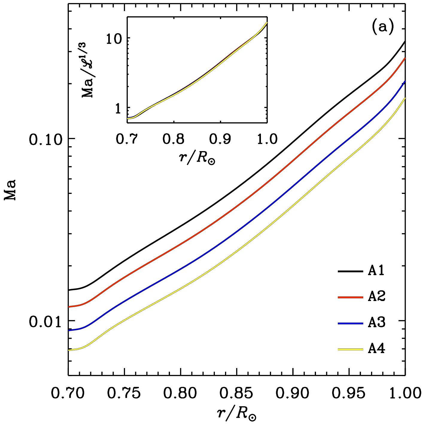
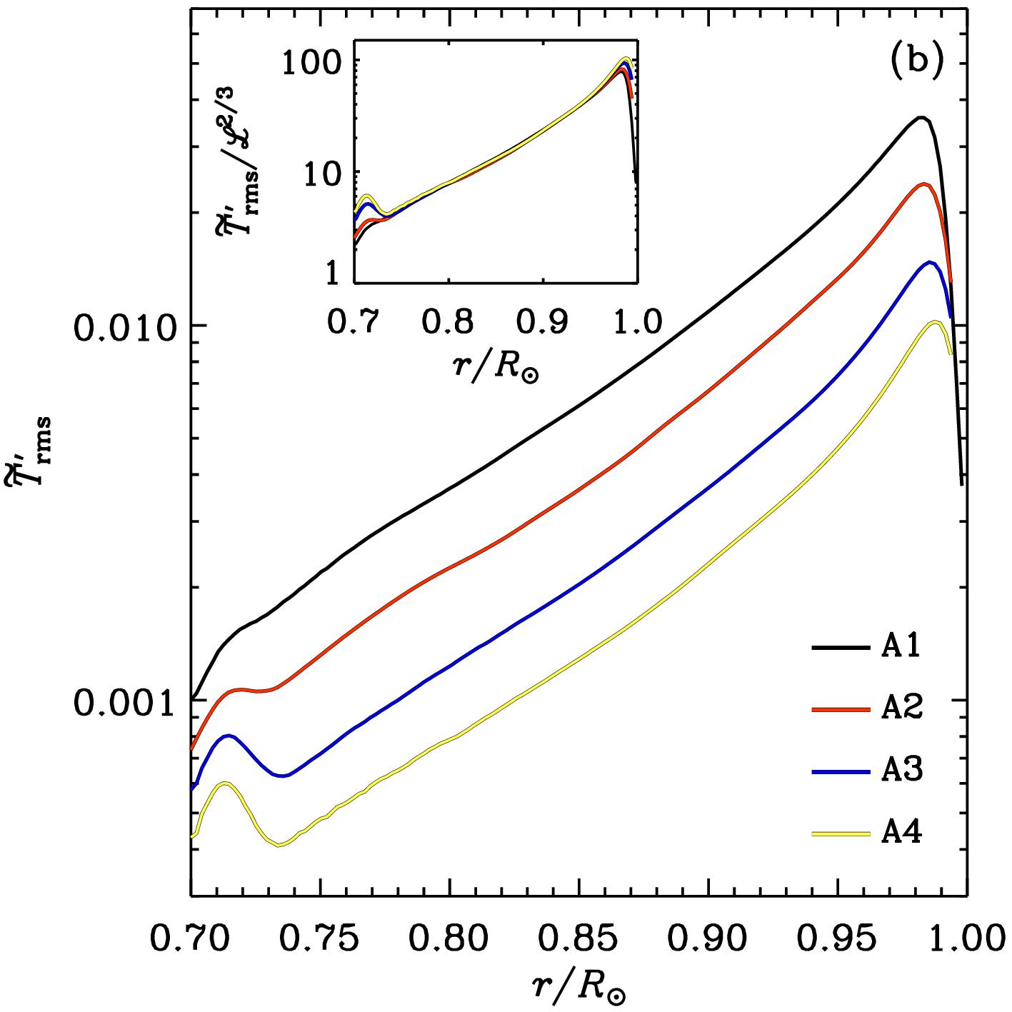
Figure 1: a) Horizontally averaged Mach number as a function of radius from Runs A1–A4. The inset shows the Mach numbers normalised by $\mathcal{L}^{1/3}$. b) Horizontally averaged normalised rms temperature fluctuation $\tilde{T}^{\prime}_{\rm rms}=T^{\prime}_{\rm rms}/\langle T\rangle_{\theta\phi}$ as a function of $r$ from the same runs. The inset shows $\tilde{T}^{\prime}_{\rm rms}$ normalised by $\mathcal{L}^{2/3}$ (colour online).

3.1 Varying luminosity

One of the disadvantages of solving the fully compressible equations is that if a realistic luminosity for the star is used, the flow velocities are much smaller than the sound speed, with the latter imposing a prohibitively short time step. In the case of the Pencil Code this has been circumvented by enhancing the luminosity by a factor that is typically on the order of $10^{5}\ldots 10^{6}$ (e.g. Käpylä et al., 2014, 2019). The luminosity enhancement procedure and the way how to relate the model results to physical units is discussed in detail in appendix 5. The ratio of the dimensionless luminosities in the simulations in comparison to the Sun quantifies this procedure:

$$L_{\rm ratio}\,=\,\mathcal{L}/\mathcal{L}_{\odot}\,.$$ (64)

Values of $L_{\rm ratio}$ quoted above are sufficiently high to decrease the thermal diffusion time such that it is possible to fully thermally relax the simulations (Käpylä et al., 2013). The downside is that the velocity as well as the fluctuations of thermodynamic quantities are unrealistically high (Warnecke et al., 2016). It has been speculated that such effects contribute to features such as convectively stable regions at certain mid-latitudes (e.g. Käpylä et al., 2011b, 2019). Here we vary the luminosity by one order of magnitude in Runs A1–A4; see table 2.3. To isolate the effects of the luminosity we keep the Reynolds and Coriolis numbers fixed by varying the viscosity $\nu$ and rotation rate of the frame ${\varOmega}_{0}$ with $\mathcal{L}^{1/3}$, see appendix 5 and table 2.3. Similarly the cooling luminosity is varied with a 1/3 power of $\mathcal{L}$.

We examine first the scaling of convective velocity and temperature fluctuations as function of the luminosity. The horizontally and temporally averaged Mach number, ${\rm Ma}=U_{\rm rms}(r)/c_{\rm s}$, is shown in figure 1(a). ${\rm Ma}$ decreases monotonically as $\mathcal{L}$ is decreased. The inset shows that the convective velocity scales with the $1/3$ power of the luminosity. Furthermore, the horizontally and temporally averaged rms value of the temperature fluctuation $T^{\prime}_{\rm rms}(r)=\sqrt{\langle T^{\prime 2}\rangle_{\theta\phi}}$, where $T^{\prime}=T-\overline{T}$, also shows a decrease with $\mathcal{L}$, and a scales with $2/3$ power of $\mathcal{L}$. Both results agree with the expected behaviour from mixing length arguments (Brandenburg et al., 2005).

The mean angular velocity profile $\overline{{\varOmega}}=\overline{U}_{\phi}/r\sin\theta+{\varOmega}_{0}$ from Run A1 is shown in figure 2(a). The rotation profile is solar-like with a fast equator, but a prominent mid-latitude minimum is also present. This is a common feature in many current simulations (e.g. Käpylä et al., 2011a; Mabuchi et al., 2015; Augustson et al., 2015; Beaudoin et al., 2018) and it is the most likely cause of the equatorward migrating large-scale magnetism observed in several MHD models of solar-like stars (Warnecke et al., 2014). Figure 2(b) shows the radial profiles of $\overline{{\varOmega}}$ from three latitudes from Runs A1–A4. We find that the rotation profiles in these runs are very similar, with the only consistent trend being the weakly decreasing equatorial rotation rate as a function of $\mathcal{L}$. Thus the Mach number has only a weak effect on the large-scale flows in the parameter range studied here.

We use the nomenclature introduced in Käpylä et al. (2017b, 2019) to classify the different radial layers in the system (see also Tremblay et al., 2015). This classification depends on the signs of the radial enthalpy flux $\overline{F}^{\rm enth}_{r}=c_{\rm P}\overline{(\rho U_{r})^{\prime}T^{\prime}}$ and the radial gradient of specific entropy, $\nabla_{r}\overline{s}=\upartial\overline{s}/\upartial r$. The buoyancy zone (BZ) is characterized by $\nabla_{r}\overline{s}<0$ and $\overline{F}^{\rm enth}_{r}>0$, whereas in the Deardorff zone (DZ), $\nabla_{r}\overline{s}>0$ and $\overline{F}^{\rm enth}_{r}>0$. Here, as emphasised by Brandenburg (2016) in the astrophysical context, the outward enthalpy flux can only be carried by Deardorff’s non-gradient contribution; see Deardorff (1966). Finally, in the overshoot zone (OZ), $\overline{F}^{\rm enth}_{r}<0$ and $\nabla_{r}\overline{s}>0$, and its bottom is located where $|\overline{F}^{\rm enth}_{r}|$ falls below a threshold value, here chosen to be $0.025L_{0}$. Figure 2(a) also shows the lower boundaries of the buoyancy, Deardorff, and overshoot zones in Run A1. We do not find a significant variation of the depths of the zones in the studied range of $\mathcal{L}$. Furthermore, a radiation zone where $|\overline{F}^{\rm enth}_{r}|\approx 0$ and $\overline{F}_{\rm rad}\approx F_{\rm tot}$, does not have room to develop in these runs and the overshoot layer tends to extend all the way to the lower boundary of the domain. Thus, it is not possible to draw conclusions about the scaling of the overshoot depth as a function of luminosity (e.g. Singh et al., 1998; Tian et al., 2009; Hotta, 2017).

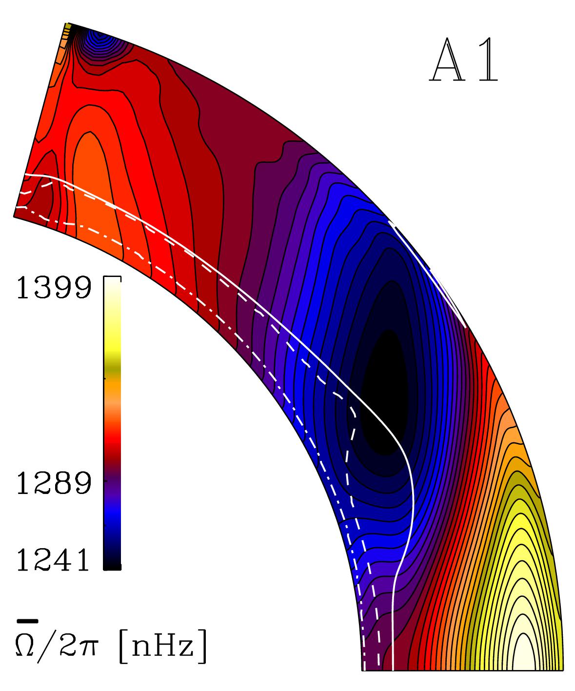
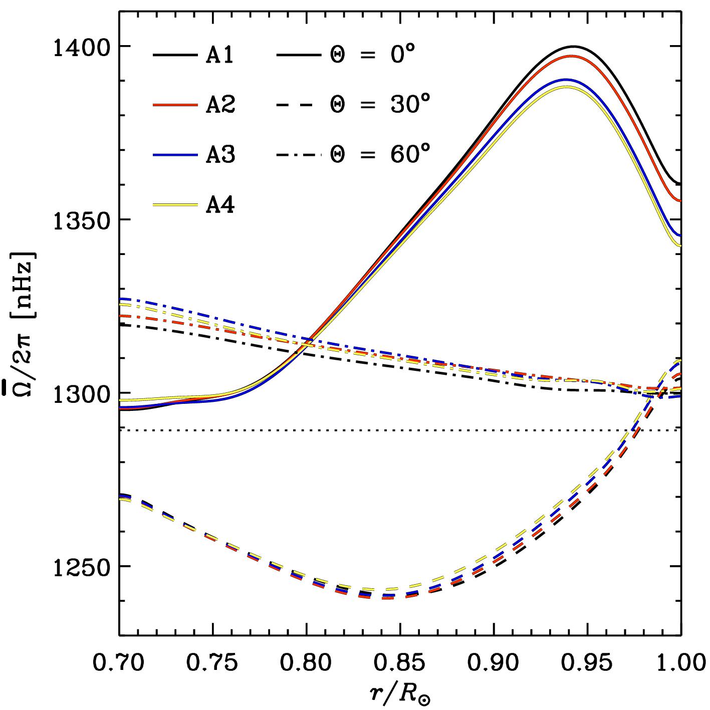
Figure 2: (a) Temporally averaged mean angular velocity $\overline{{\varOmega}}=\overline{U}_{\phi}/r\sin\theta+{\varOmega}_{0}$ from Run A1. The white solid, dashed, and dot-dashed lines denote the bottoms of the BZ, DZ, and OZ, respectively. (b) $\overline{{\varOmega}}$ from latitudes $0^{\circ}$ (solid lines), $30^{\circ}$ (dashed), and $60^{\circ}$ (dash-dotted) for Runs A1 (black), A2 (red), A3 (blue), and A4 (yellow) (colour online).

The contours of angular velocity are clearly inclined with respect to the rotation vector in Runs A1–A4, which indicates deviation from the Taylor-Proudman balance. To study this, we consider the vorticity equation in the meridional plane:

$$\frac{\upartial\overline{\omega}_{\phi}}{\upartial t}\,=\,r\sin\theta\frac{\upartial\overline{{\varOmega}}^{2}}{\upartial z}+(\bm\nabla\overline{T}\times\bm\nabla\overline{s})_{\phi}+\cdots\,,$$ (65)

where $\overline{\bm\omega}=\bm\nabla\times\overline{\bm U}$, and where $\upartial/\upartial z=\cos\theta\,\upartial/\upartial r-r^{-1}\sin\theta\,\upartial/\upartial\theta$ is the derivative along the axis of rotation. The dots denote contributions from the Reynolds stress and molecular viscosity (e.g. Warnecke et al., 2016). The first term on the rhs describes the effect of rotation, essentially the Coriolis force, on the mean flow, whereas the second term corresponds to the baroclinic effect, which results from latitudinal gradients of thermodynamic quantities. In a perfect Taylor-Proudman balance the baroclinic term vanishes and the isocontours of $\overline{{\varOmega}}$ are cylindrical, corresponding to $\upartial\overline{{\varOmega}}/\upartial z=0$.

Meridional cuts of the two terms on the right-hand side of (65) from Run A1 are shown in figure 3. We find that the two terms tend to balance in the bulk of the convection zone with larger deviations occurring mostly near the surface. The current simulations do not resolve the surface layers to a high enough degree to capture the Reynolds stress-dominated region that is expected to occur there (e.g. Hotta et al., 2015). Figure 4 shows the Coriolis and baroclinic terms as functions of latitude at the middle of the domain $r=0.85R_{\odot}$ for Runs A1–A4. In accordance with the similarity of the rotation profiles, also the terms contributing to the baroclinic balance are very similar in these runs; the only clear trend is a slight decrease in the near-equator regions for both terms. Thus, we conclude that the main effect of the decreasing luminosity is a decrease in the Mach number, but this has only a weak influence on the large-scale dynamics.

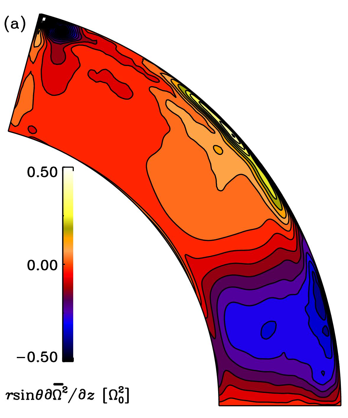
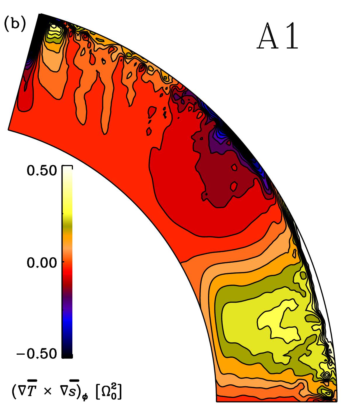
Figure 3: (a) Coriolis term from the mean vorticity equation (65) from Run A1 as a function of radius and latitude (b) The same as (a) but for the baroclinic term (colour online).

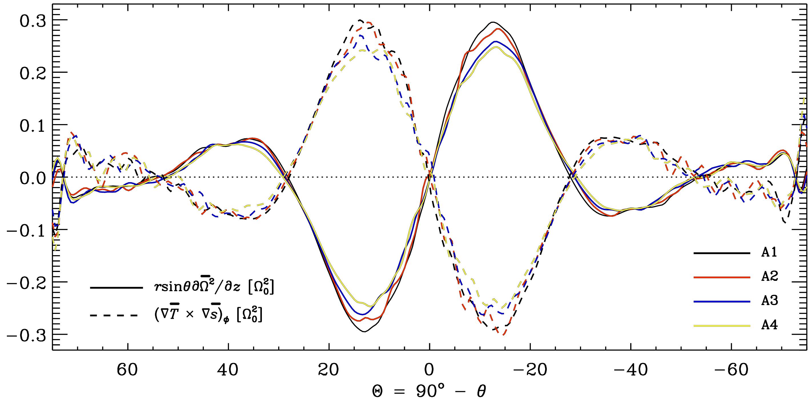
Figure 4: Coriolis (solid lines) and baroclinic (dashed) terms as functions of latitude $\Theta=90^{\circ}-\theta$ at the middle of the domain ($r=0.85R_{\odot}$) from Runs A1 (black), A2 (red), A3 (blue), and A4 (yellow) (colour online).

3.2 Influence of the centrifugal force

Typical stellar convection simulations either omit the contribution of the centrifugal force or they consider it to be subsumed in the gravitational force. This is also true for Pencil Code models, where the issue is more severe due to the enhanced rotation rate. Here we study the influence of $\mathscrbf{F}^{\rm cent}$ for the first time in Pencil Code simulations in spherical wedges.

We have introduced a parameter $c_{\rm cent}$ in front of the centrifugal force in equation (8), with which it is possible to regulate its strength. It is defined such that

$$c_{\rm cent}\,=\,\bigl{|}\mathscrbf{F}^{\rm cent}\bigr{|}\big{/}\bigl{|}\mathscrbf{F}^{\rm cent}_{0}\bigr{|}\,,$$ (66)

where $\mathscrbf{F}^{\rm cent}_{0}$ is the unaltered magnitude of the centrifugal force. Such a procedure is used because the actual force in the simulations would be much stronger than in the Sun, for example. This is due to the enhanced luminosity and rotation rate. Furthermore, the initial condition is spherically symmetric and does not take the centrifugal potential into account. Such a combination would lead to a violent readjustment in the early stage of the simulation if $c_{\rm cent}=1$ was used.

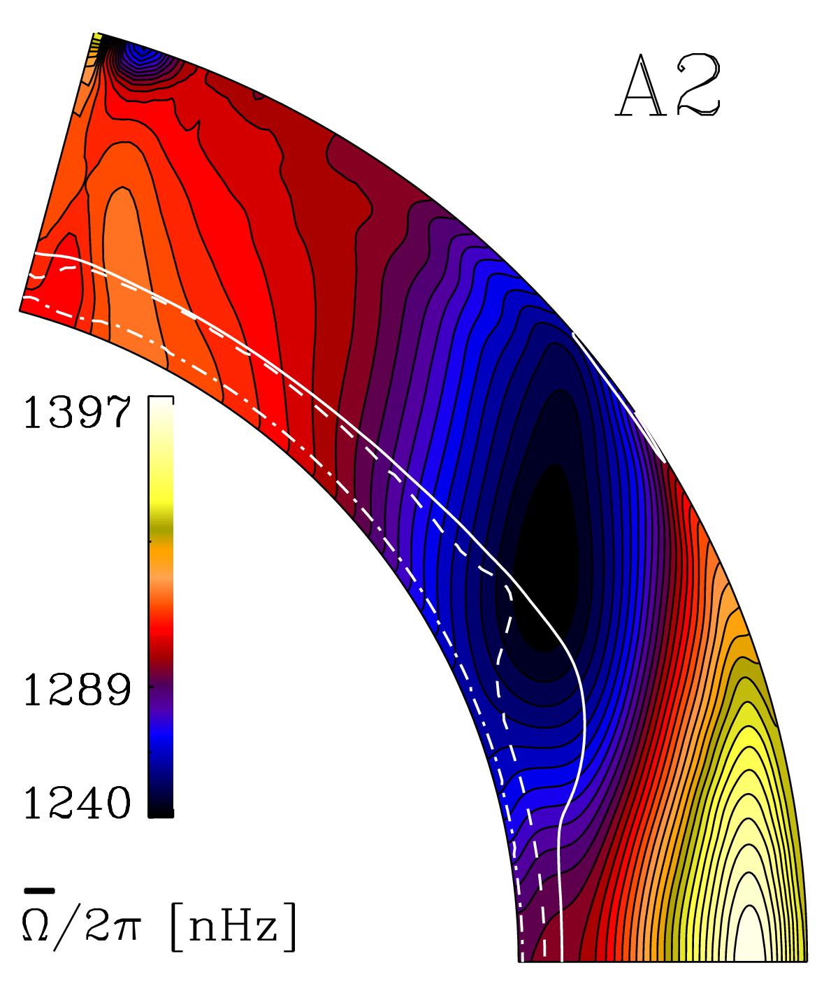
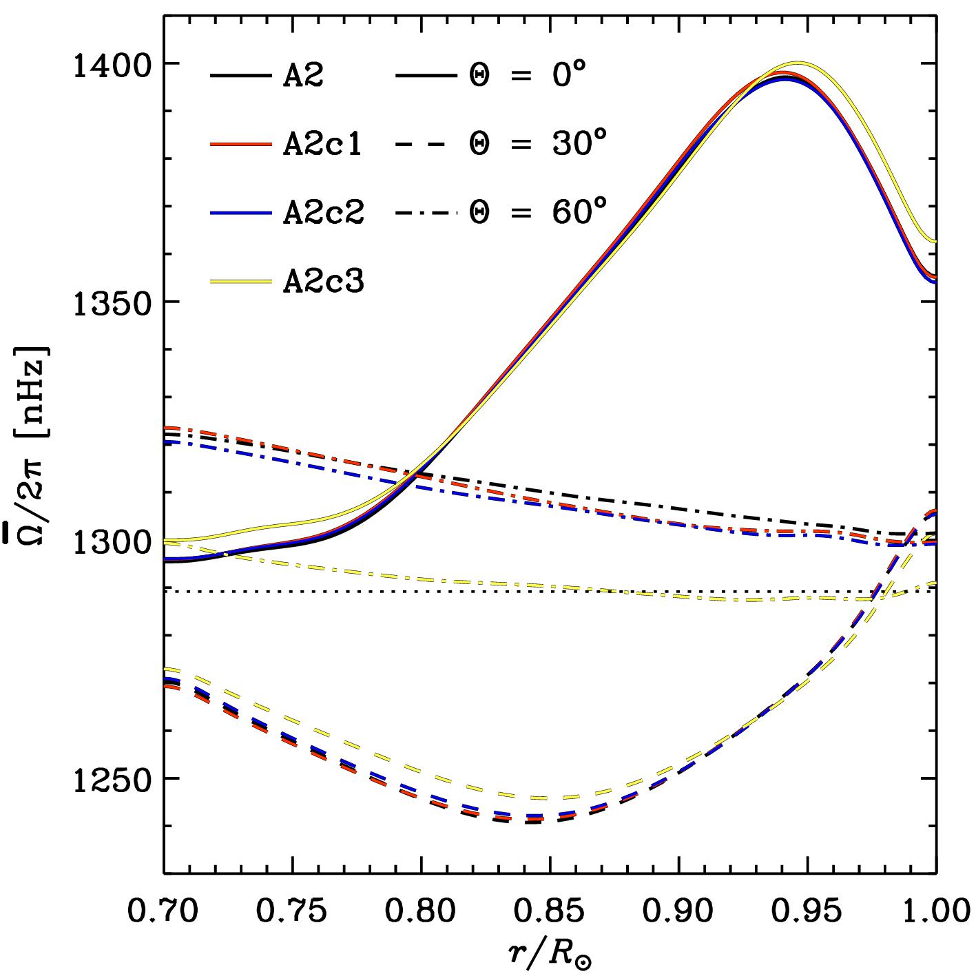
Figure 5: Same as figure 2 but for Runs A2 (black), A2c1 (red), A2c2 (blue), and A2c3 (yellow) (colour online).

We consider three cases where $c_{\rm cent}$ obtain values $5\cdot 10^{-4}$, $5\cdot 10^{-3}$, and $0.05$ (Runs A2c1, A2c2, and A2c3 in table 2.3) and compare those to a run with $c_{\rm cent}=0$ (Run A2). Considering the ratio of the centrifugal force and the acceleration due to gravity at the stellar surface at the equator, these values translate to

$$\bigl{|}\mathscrbf{F}^{\rm cent}\bigr{|}\big{/}\bigl{|}\mathscrbf{F}^{\rm grav}\bigr{|}\,\approx\,2\cdot 10^{-4}\ldots 0.02\,.$$ (67)

These are to be compared with the corresponding solar value,

$$\bigl{|}\mathscrbf{F}^{\rm cent}_{\odot}\bigr{|}\big{/}\bigl{|}\mathscrbf{F}^{\rm grav}_{\odot}\bigr{|}\,=\,{\varOmega}^{2}_{\odot}R_{\odot}/g_{\odot}\approx 2\cdot 10^{-5}\,.$$ (68)

Thus even the lowest value of $c_{\rm cent}$ considered here corresponds to a relative strength of the centrifugal force that is an order of magnitude greater than in the Sun.

In figure 5 we compare the rotation profiles of the runs where $c_{\rm cent}\neq 0$ with that of Run A2. We find that the differences are minor with the exception of the high latitudes ($\Theta=60^{\circ}$) for Run A2c3. The effect is relatively minor even in this case, and considering that the magnitude of the centrifugal force is already three orders of magnitude greater than in the Sun, we estimate that its effect is likely to be minor in real stars. We note, however, that the cooling applied in the current simulations is spherically symmetric and it is likely to work against the centrifugal force.

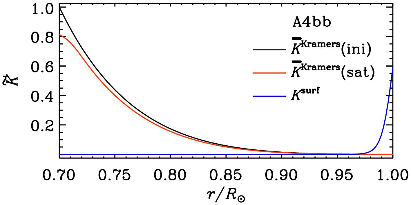
Figure 6: Initial (black) and saturated (red) profiles of $\overline{K}^{\rm Kramers}$ and $K^{\rm surf}$ (blue) from Run A4bb (colour online).

3.3 Influence of thermal BCs

Various thermal BCs and treatments of the unresolved photosphere have been used in the literature. For example, the ASH simulations often apply a constant entropy gradient (Brun et al., 2004; Brown et al., 2008) or a constant value of specific entropy at the surface (Nelson et al., 2018). Furthermore, the energy flux is carried through the upper surface via SGS entropy diffusion (e.g. Augustson et al., 2012). Similar conditions are used also by Fan and Fang (2014), whereas Hotta et al. (2014) and their following work assume zero radial gradient of the entropy. Several other anelastic simulations assume a constant entropy on both radial boundaries (e.g. Gastine et al., 2012; Simitev et al., 2015). Another approach is to apply a constant temperature (Käpylä et al., 2010; Mabuchi et al., 2015) or a black body condition (e.g. Käpylä et al., 2011a), where the former is typically associated with a cooling applied near the surface. In the latter, the flux at the surface is carried again by SGS diffusion.

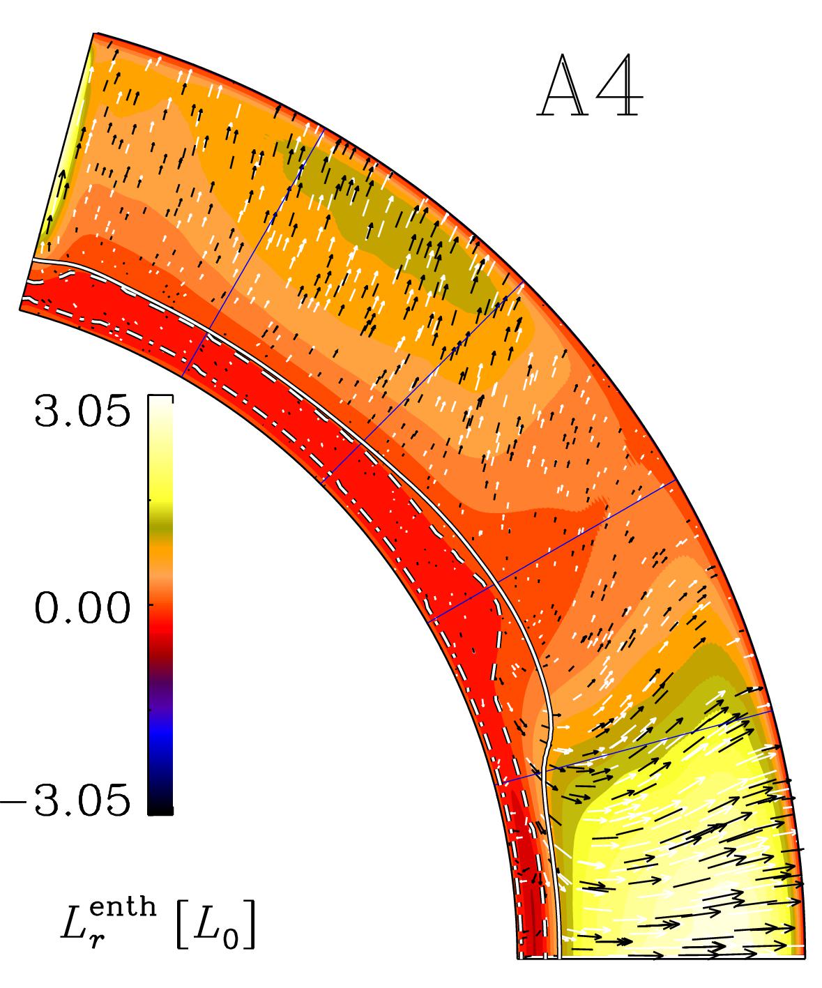
(a) A4

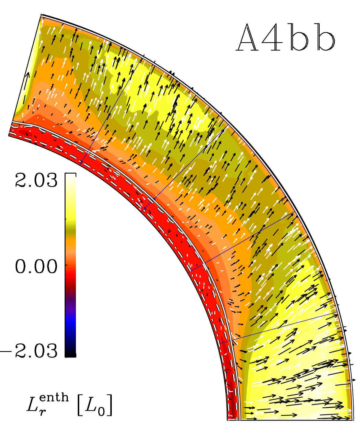
(b) A4bb

Figure 7: Radial enthalpy flux (colours) and the vectorial enthalpy flux (arrows) from Runs A4 and A4bb. The solid, dashed, and dot-dashed black and white lines indicate the bottoms of the BZ, DZ, and OZ, respectively (colour online).

We consider two main setups where we either apply cooling in a shallow layer with a constant temperature [cT, Eq. (31)] imposed at the surface (Run A4) or enhanced radiative heat conductivity $K^{\rm surf}$ near the surface (see figure 6) in conjunction with a black body [bb, Eq. (32)] condition (Run A4bb). Both runs were repeated with a vanishing entropy gradient at the surface (Runs A4ds and A4ds2, respectively).

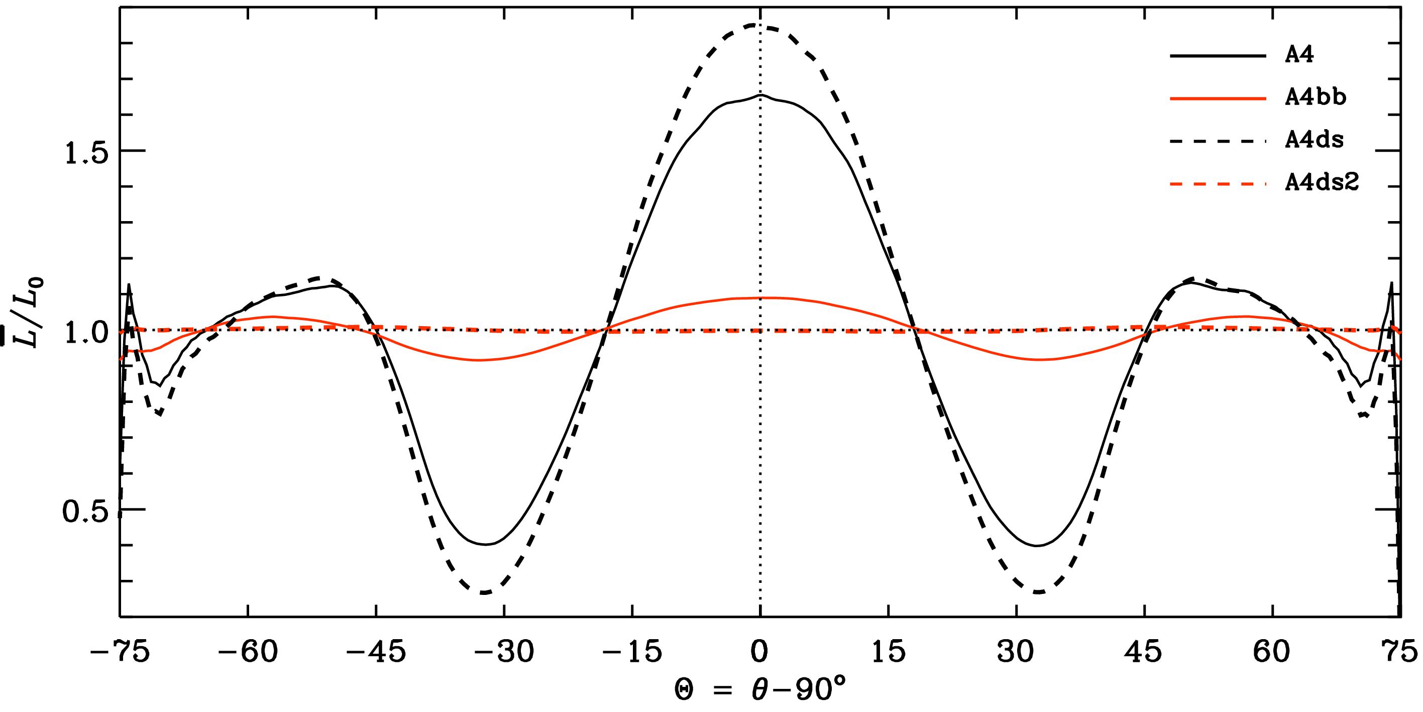
Figure 8: The total time averaged luminosity at $r=R_{\odot}$ from Runs A4 (black solid line) and A4bb (red solid), A4ds (black dashed), and A4ds2 (red dashed) (colour online).

The convective energy transport, quantified by the luminosity of the radial enthalpy flux $L_{r}^{\rm enth}=4\pi r^{2}\overline{F}^{\rm enth}_{r}$, is highly anisotropic in Run A4 with the surface cooling and constant temperature BC; see figure 7(a). Furthermore, the latitudinal variation of the depth of the buoyancy, overshoot, and Deardorff zones is substantial. We also note the very weak convection around $\Theta=30^{\circ}$. An earlier study (Käpylä et al., 2019) has shown that in an otherwise identical setup, but where a fixed profile of $K$ is used, leads to a situation where only a very thin surface layer is convectively unstable (e.g. their Run MHDp). In Run A4bb, the black body condition is used in addition to enhanced radiative diffusion near the surface, transporting the energy through the surface. In this case the convective energy transport is clearly less anisotropic than in Run A4, although substantial latitudinal variation still occurs; see figure 7(b). Furthermore, figure 8 shows that the surface luminosity varies much more in Run A4 than in Run A4bb. The extreme latitude dependence in Run A4 can be explained by the fact that the flux near the surface is determined by the difference between a fixed spherically symmetric profile of the temperature $T_{\rm cool}$ and the dynamically evolving actual temperature $T$:

$$F_{r}^{\rm cool}\,=\,\int_{r_{0}}^{R_{\odot}}{\varGamma}_{\rm cool}\,{\rm d}r\,=\,-\,{\varGamma}_{0}\int_{r_{0}}^{R_{\odot}}f(r)(T_{\rm cool}-\langle T\rangle_{\theta\phi})\,{\rm d}r\,.$$ (69)

Note that in the cases with surface cooling, the radiative flux at the surface is negligible and $L^{\rm cool}=4\pi r_{1}^{2}F_{r}^{\rm cool}\approx L_{0}$. At mid-latitudes, the actual temperature has a local minimum, and the cooling due to the relaxation term in the entropy equation becomes inefficient, as seen in figure 8. This leads to a more stable thermal stratification at mid-latitudes ($20\lesssim|\Theta|\lesssim 45$). The situation is qualitatively similar although the latitudinal variation is even slightly enhanced in Run A4ds where a vanishing radial entropy gradient is enforced at the surface.

In the case of Run A4bb, however, the flux is carried by radiative diffusion near the surface, which is proportional to the radial derivative of the temperature, which varies much less as a function of latitude than the difference between a fixed reference temperature and the actual value of $T$. There is still substantial latitudinal variation, on the order of 10 per cent of the total luminosity. This is due to the non-linear nature of the black body BC, see equation (32):

$$-K^{\rm tot}\frac{\upartial T}{\upartial r}\,=\,\sigma T^{4}\,,$$ (70)

where $K^{\rm tot}=K^{\rm Kramers}+K^{\rm surf}$. In practise $K^{\rm Kramers}\ll K^{\rm surf}$ near the surface and $F_{r}^{\rm rad}\approx-K^{\rm surf}{\upartial T}/{\upartial r}$. However, adopting the ‘ds’ BC (Run A4ds2) leads, under the assumption of hydrostatic equilibrium, to ${\upartial T}/{\upartial r}=g/c_{\rm P}$ which is independent of latitude and time. This implies that the radiative (=total) flux is fixed at both boundaries which is indeed reproduced by the simulation, see the red dashed line in figure 8. However, the total energy in this simulation does not find a saturated state but a constant drift is observed as a function of time. This is an issue related to having von Neumann type BCs at both boundaries. We find that the choice of thermal BC has a relatively minor effect on the surface luminosity and that the results are more sensitive to the parameterisation of the photospheric physics. The only exception is the case where a constant radiative flux is imposed at both boundaries (Run A4ds2) which leads to an unphysical drift of the total energy of the solution.

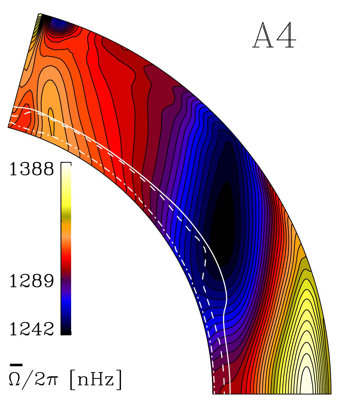
(a) A4

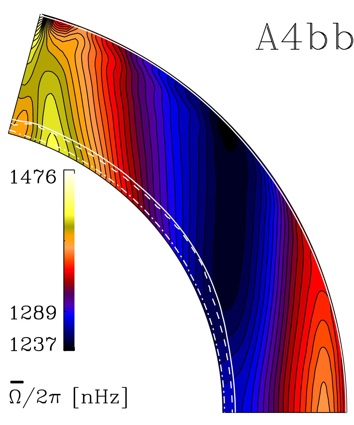
(b) A4bb

Figure 9: Temporally averaged mean angular velocity $\overline{{\varOmega}}=\overline{U}_{\phi}/r\sin\theta+{\varOmega}_{0}$ from Runs A4 and A4bb (colour online).

We find a substantial poleward contribution to the heat flux in all rotating cases; see the arrows for $\overline{\bm{F}}^{\rm enth}=(\overline{F}^{\rm enth}_{r},\overline{F}^{\rm enth}_{\theta},0)$ in figure 7. The tendency for the enthalpy flux to align with the rotation vector is an established result from mean-field theory of hydrodynamics (Rüdiger, 1989; Kitchatinov et al., 1994). Furthermore, mean-field models have shown that such poleward flux is instrumental in producing a pole-equator temperature difference that can break the Taylor-Proudman balance (Brandenburg et al., 1992).

The rotation profiles from Runs A4 and A4bb are shown in figure 9. We find that the cases with surface cooling deviate more strongly from the Taylor-Proudman balance. Furthermore, the latitudinal variation of the bottom of the buoyancy and overshoot zones are more pronounced in these cases. The runs with diffusive transport of thermal energy near the surface also tend to exhibit strong polar vortices. However, this feature is likely to be dependent on the initial conditions or the history of the run, as was shown by Gastine et al. (2014) and Käpylä et al. (2014). We again find that the choice of BC is less important than the treatment of the photosphere. The rotation profiles of Runs A4 and A4ds are practically identical despite the different boundary conditions. The averaged angular velocities in Runs A4bb and A4ds2 are also qualitatively similar, despite the fact that the kinetic energy in the latter is slowly increasing.

3.4 Influence of magnetic BCs

Here we compare the dynamo solution of Run M1 from Käpylä et al. (2016) with the vE magnetic BC with a corresponding Run M2 with the vJ BC of Gent et al. (2017). While the vE conditions assume that the electric field vanishes, they allow non-vanishing horizontal currents on the boundary. The vJ conditions assume that also the currents vanish on the boundary. In spherical coordinates the tangential components of the current density are given by

$$J_{\theta}\,=\, \,\dfrac{1}{r^{2}\sin\theta}\dfrac{\upartial^{2}A_{\phi}}{\upartial\theta\upartial\phi}+\dfrac{\cot\theta}{r^{2}\sin\theta}\dfrac{\upartial A_{\phi}}{\upartial\phi}-\dfrac{1}{r^{2}\sin^{2}\theta}\dfrac{\upartial^{2}A_{\theta}}{\upartial\phi^{2}}$$

$$\hskip 65.44133pt-\dfrac{\upartial^{2}A_{\theta}}{\upartial r^{2}}-\dfrac{2}{r}\dfrac{\upartial A_{\theta}}{\upartial r}+\dfrac{1}{r}\dfrac{\upartial^{2}A_{r}}{\upartial r\upartial\theta}\,,$$

$$J_{\phi}\,=\, \,\dfrac{1}{r^{2}\sin\theta}\left(\dfrac{A_{\phi}}{\sin\theta}-\cos\theta\dfrac{\upartial A_{\phi}}{\upartial\theta}-\cot\theta\dfrac{\upartial A_{\theta}}{\upartial\phi}+\dfrac{\upartial^{2}A_{\theta}}{\upartial\theta\upartial\phi}+r\dfrac{\upartial^{2}A_{r}}{\upartial r\upartial\phi}\right)$$

$$\hskip 65.44133pt-\dfrac{\upartial^{2}A_{\phi}}{\upartial r^{2}}-\dfrac{2}{r}\dfrac{\upartial A_{\phi}}{\upartial r}-\dfrac{1}{r^{2}}\dfrac{\upartial^{2}A_{\phi}}{\upartial\theta^{2}}\,.$$

The terms involving $A_{r}$ vanish on the boundary under the condition ${\upartial A_{r}}/{\upartial r}=0$. Setting $A_{\theta}$ and $A_{\phi}$ constant on the boundary (e.g., 0), eliminates the remaining terms involving the tangential derivatives, see equation (34). There remains an additional constraint for the horizontal components of ${\bm A}$ satisfying

$$\dfrac{\upartial^{2}A_{\theta}}{\upartial r^{2}}+\dfrac{2}{r}\dfrac{\upartial A_{\theta}}{\upartial r}\,=\,0\,,\hskip 56.9055pt\dfrac{\upartial^{2}A_{\phi}}{\upartial r^{2}}+\dfrac{2}{r}\dfrac{\upartial A_{\phi}}{\upartial r}\,=\,0\,.$$ (71)

We recognize that this is technically over-determined, with five BCs on three equations, and a more general solution to the BC would be desirable.

Apart from the BCs, the models differ through the inclusion of a set of test fields (see e.g., Schrinner et al., 2005, 2007; Warnecke et al., 2018). These are used to extract numerically the turbulent transport coefficients responsible for the evolution of large-scale magnetic fields in the framework of mean-field dynamo theory (e.g. Moffatt, 1978; Krause and Rädler, 1980). The test fields are acted upon by the flow, generated by the MHD solution, but, unlike the physical magnetic field, there can be no feedback on the flow nor on the energy via Lorentz force and Ohmic heating, respectively. The solution should therefore be independent of the test fields. However, the Courant condition is also applicable to the evolution of the test fields and typically necessitates a slightly reduced time step. Due to the chaotic nature of such a system, the details of the solutions diverge, but the statistical properties such as cycle lengths remain consistent.

To examine the potential differences in the solutions accounted for by the BCs, we consider equally long and similar epochs in the dynamo solutions for both models. The chosen epoch represents a solar-like state of the solutions. Such states occur at different times in the two simulations due to the changes in the length of the time step. In this context we mean by ‘solar-like’ that near the surface the azimuthal magnetic field exhibits a regular equatorward drift in lower latitudes and poleward drift in higher latitudes. The magnetic field shows cyclic polarity reversals and typically has opposite signs on the two hemispheres (antisymmetric with respect to the equator). As has been described in detail in Käpylä et al. (2016), such regular epochs are rather rare in these simulations, as especially the parity can undergo changes to nearly symmetric solutions (i.e., the same orientation of the toroidal field in both hemispheres), the migration patterns, however, remaining unaltered.

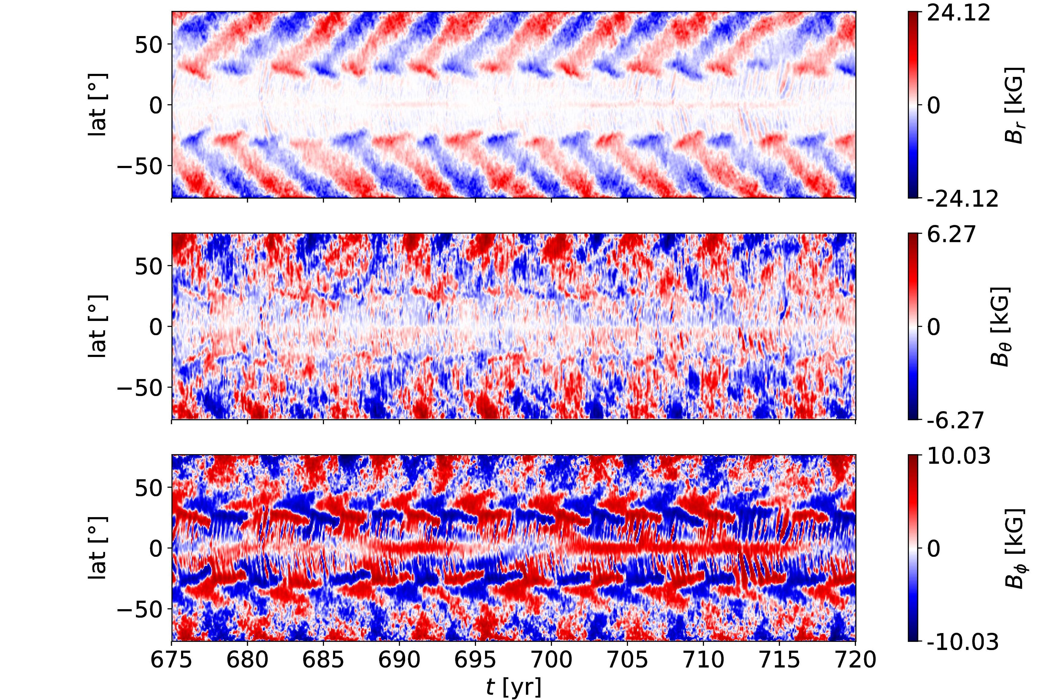
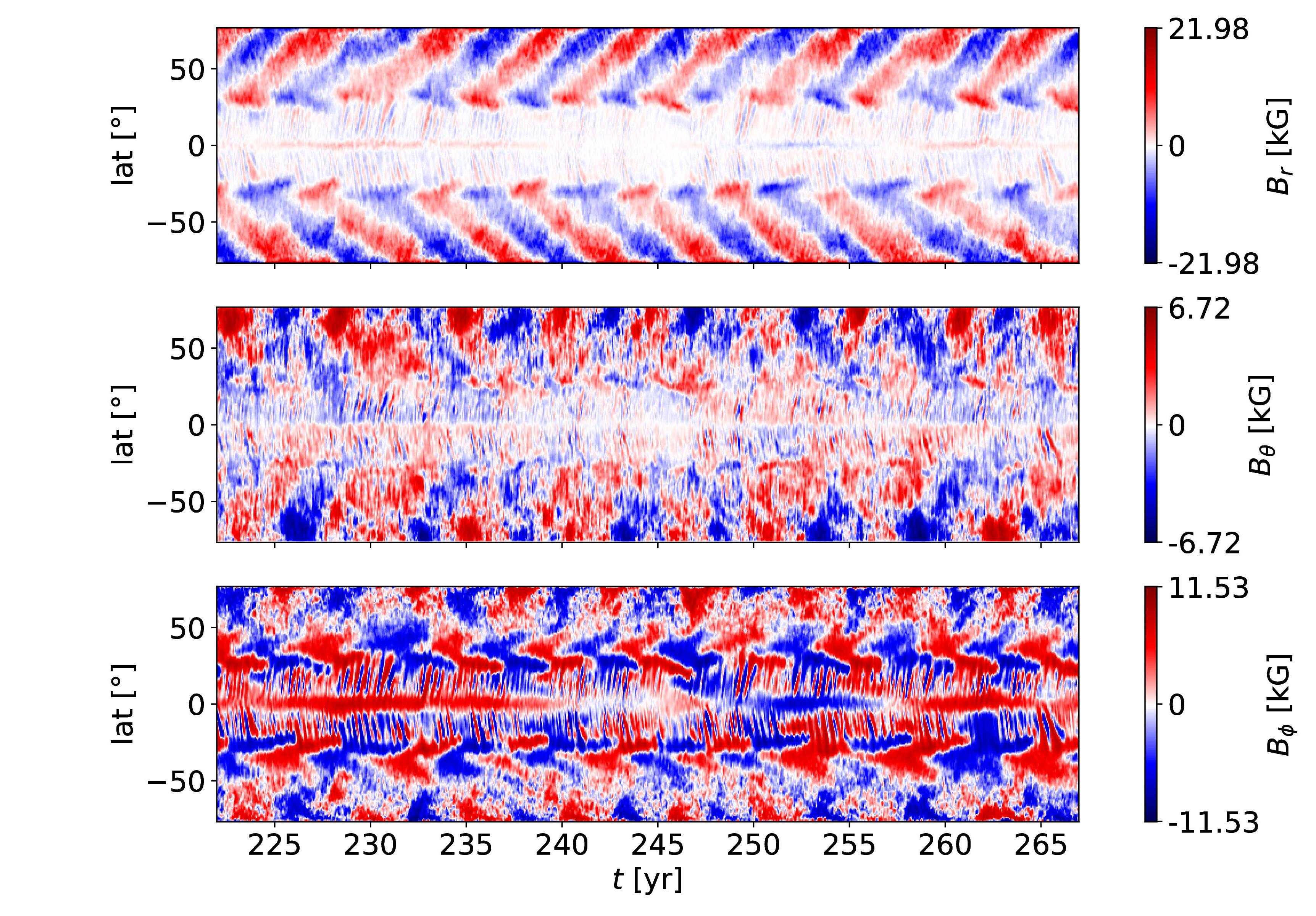
Figure 10: Near-surface ($r=0.98R_{\odot}$) magnetic field butterfly diagrams from Runs M1 (top) and M2 (bottom) (colour online).

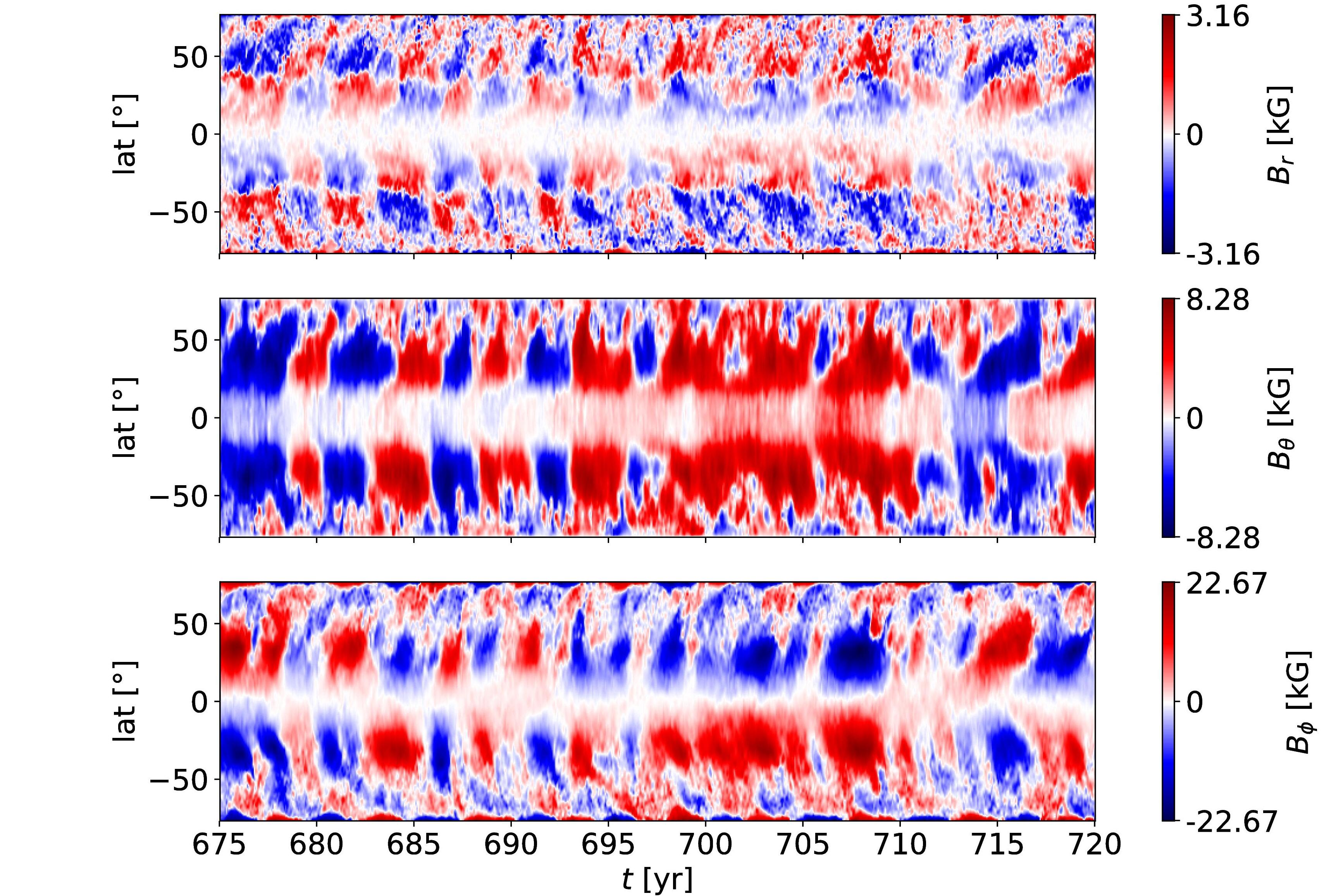
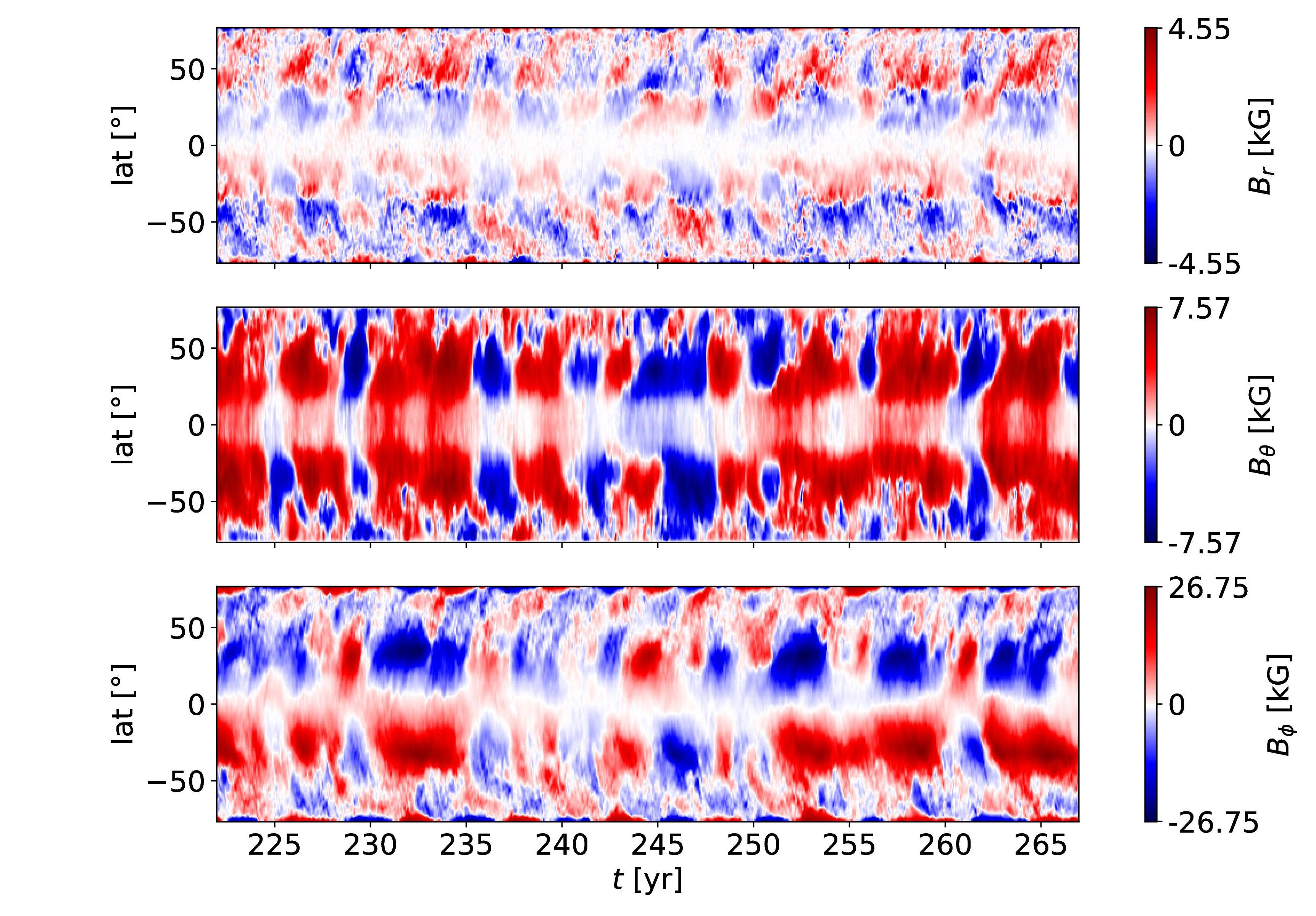
Figure 11: Base ($r=0.72R_{\odot}$) magnetic field butterfly diagrams from Runs M1 (top) and M2 (bottom) (colour online).

Figure 10 depicts the solar-like solution near the surface of the convection zone, $r=0.98R_{\odot}$ by magnetic field component from each of Runs M1 with vE BCs (upper three panels) and M2 with vJ BCs (lower three panels). As is evident from figure 10, the runs with different boundary conditions do not differ much. Also, the cycle period in Run M2 appears slightly longer than in M1, while the amplitude of the magnetic field is nearly unaffected.

We might expect the differences in the boundary conditions to be most apparent near the base of the convection zone, hence in figure 11 we show time-latitude diagrams close to the boundary in each Run M1 and M2 at $r=0.72R_{\odot}$. There, we see two different incarnations of the long-period, nearly purely antisymmetric, dynamo cycle described in detail by Käpylä et al. (2016). Hence, the effect of the BCs on the overall dynamo solution are very small, and part of the variation seen here is also likely to arise from the intrinsically chaotic nature of the solutions.

As an additional check on the impact of the BCs on the solution, we also compare the evolution of the rms of the azimuthally averaged magnetic field strength in Runs M1 and M2 during this 45 year period near the boundary. The layer $r<0.73R_{\odot}$ is considered and the time evolution plotted in figure 12. The common time is initialised to zero for the purposes of the plot. The temporal averages for $B_{\rm rms}$, during this period were computed as 4.37 kG and 4.57 kG with standard deviation of 1.07 kG and 1.45 kG for M1 and M2, respectively. This is a rather small difference, as we already concluded from the time-latitude diagrams.

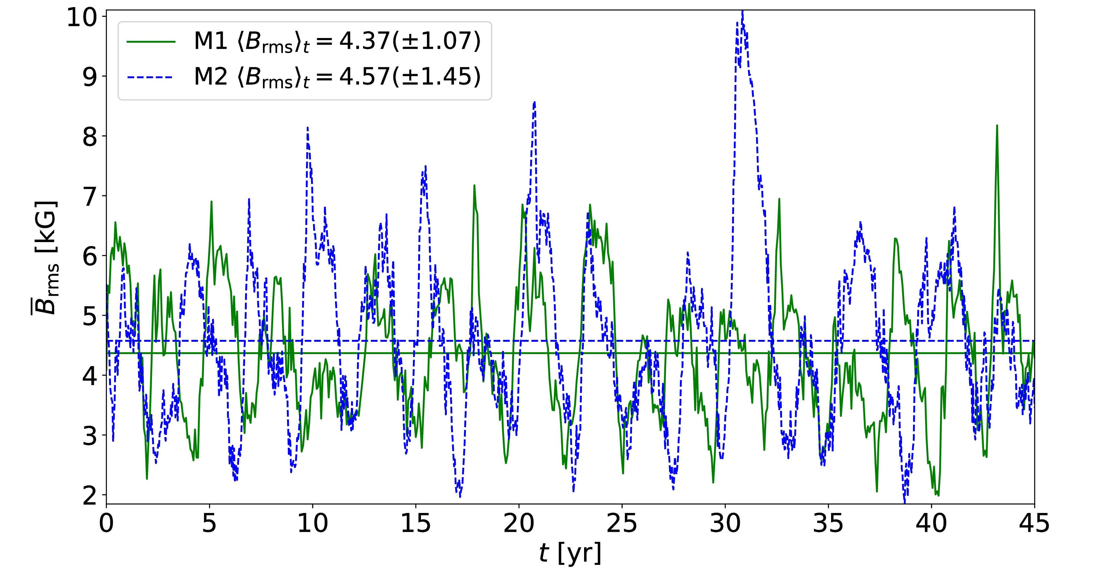
Figure 12: Comparison of azimuthally averaged magnetic field (rms) near the base of the convection zone ($r<0.73R_{\odot}$) between Runs M1 (green, solid) and M2 (blue, dashed) during the respective 45-year time intervals 222–267 and 675–720 years (colour online).

Figure 13: Comparison of the $D^{2}$ spectra of azimuthally averaged $B_{\phi}$ for Runs M1 (top) and M2 (bottom). Panel (a) corresponds to north, (b) to south, and (c) to full latitudinal extent (colour online).

To reveal the differences in more detail, we repeat the analysis used to determine the basic dynamo period and parity of the two runs described extensively in Käpylä et al. (2016) and Olspert et al. (2016). For the cycle period estimation we used the $D^{2}$ statistic of Pelt (1983), which is extended to suit quasi-periodic time series. Additional to the frequency, the statistic includes a free parameter called coherence time (or time-scale), which quantifies the degree of non-periodicity. $D^{2}$ spectrum for the azimuthal component of the magnetic field over the whole time interval of the runs, depicted in figure 13, reveals that the basic cycle is indeed somewhat longer for Run M2 than for M1.

In Olspert et al. (2016) we reported a peculiar feature of hemispheric asymmetry, namely the cycle periods being different for different hemispheres, and this behaviour is now seen to persist also with a different magnetic boundary condition. The cycle periods for Run M2 are 5.27 yr and 5.22 yr for north and south, respectively. The corresponding values for Run M1 are 5.17 yr and 5.02 yr. In the horizontal axis of the figure we also plot the ratio of the coherence time to the period $l_{\rm coh}$. From this figure, it is evident that the cycle for Run M2 is somewhat less coherent compared to that of M1. The last thing to note from this figure is that the average cycle amplitude is slightly lower for Run M2 than for M1.

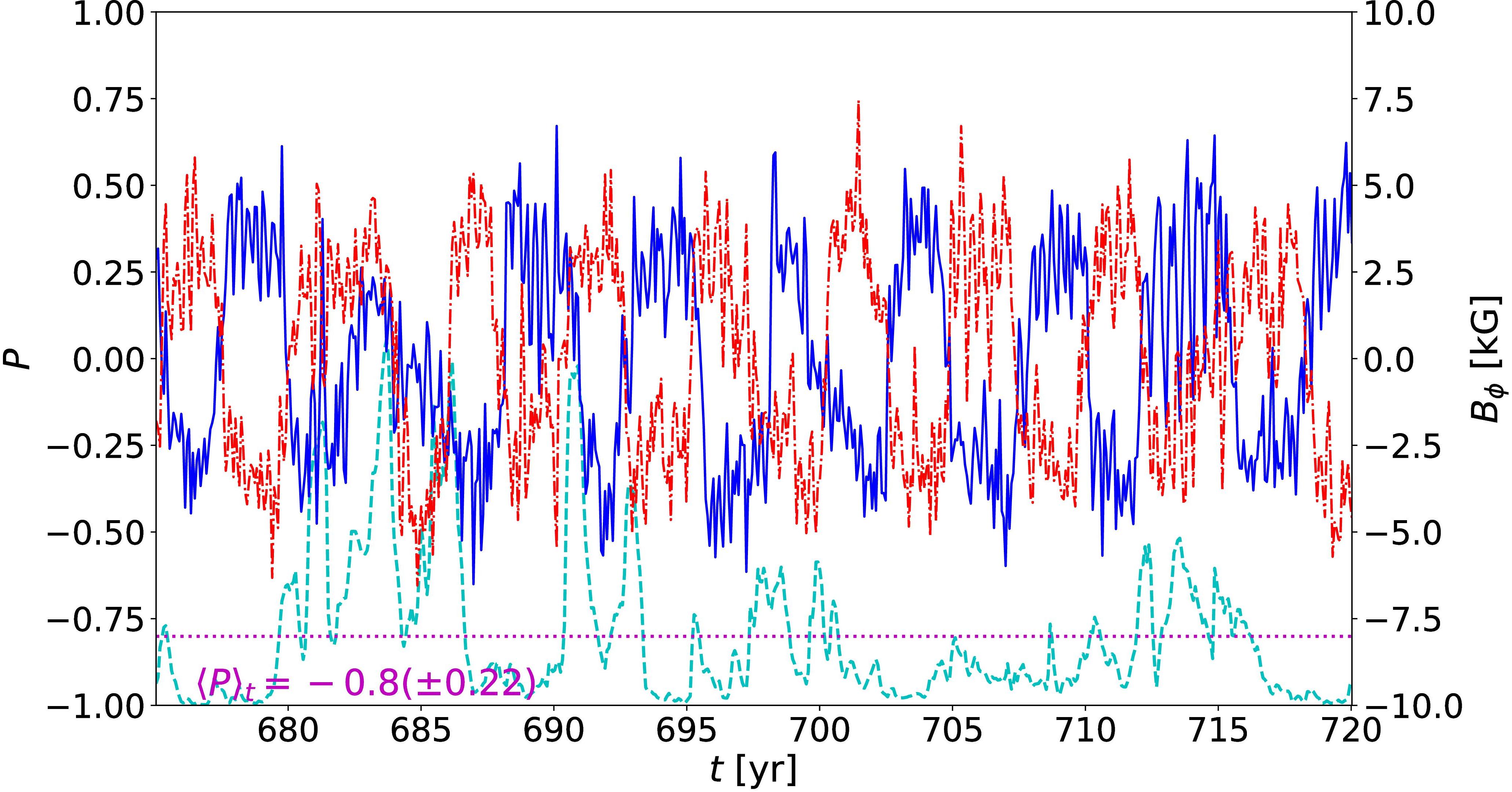
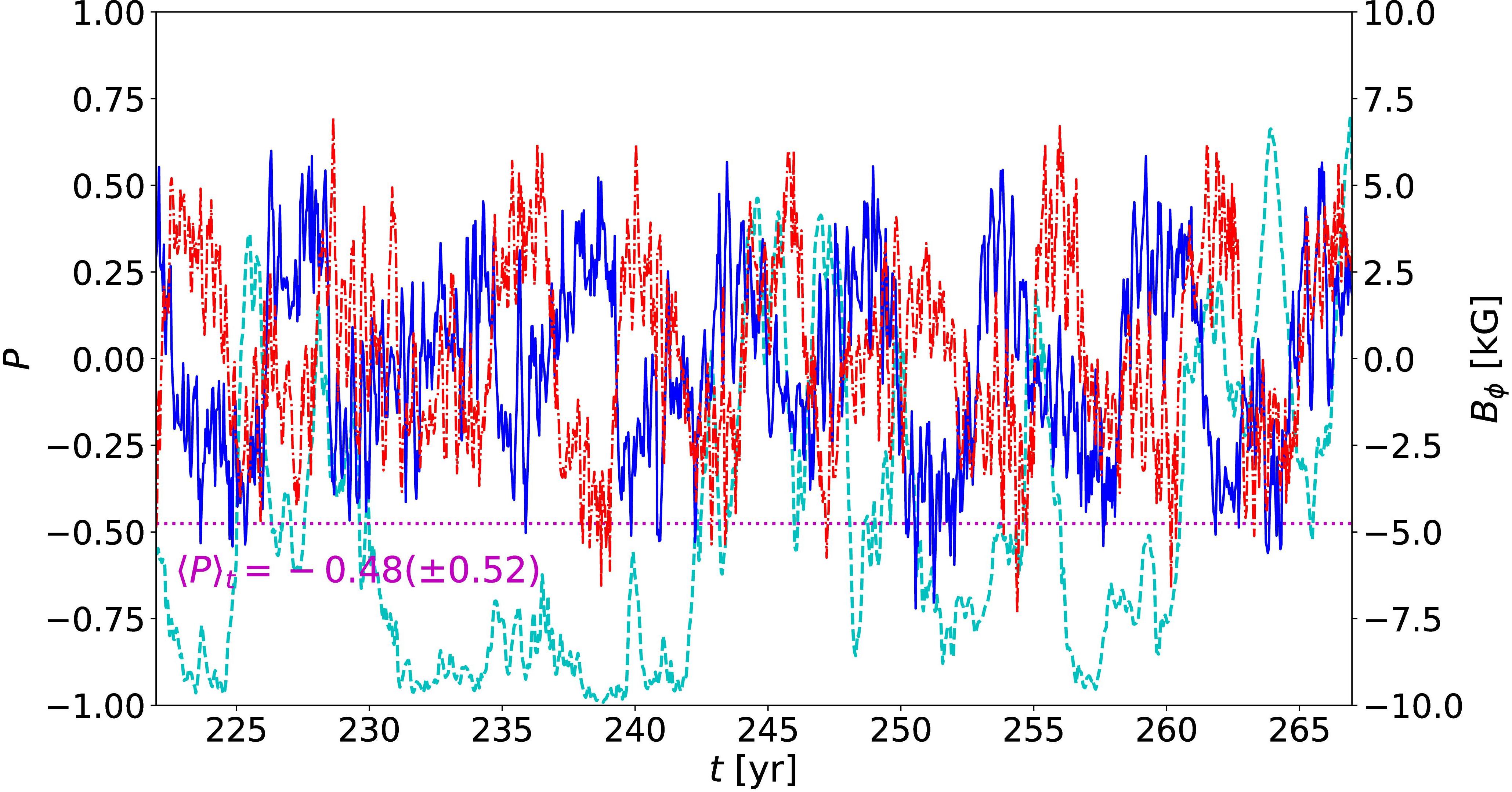
Figure 14: Top panel: global instantaneous parity (cyan, dashed) and its temporal average (magenta, dotted) from Run M2. Zoom-in over 45 years of same parity (cyan, dashed) and the 45 year temporal average from Run M1 (middle) and similar period from Run M2 (bottom), together with azimuthally averaged toroidal magnetic field near the surface ($r=0.98R_{\odot}$) at $\pm 25\degree$ (blue, solid: north, red, dash-dotted: south) (colour online).

We have over 1000 years of data from Run M1 and almost 1000 years for M2. More detailed comparison of the full data sets including test-field analysis is planned elsewhere. In the top panel of figure 14 we provide the time evolution of the global parity for the full duration of Run M2 for comparison with Fig 13(a) of Käpylä et al. (2016), where the first 440 years of Run M1 was presented. Parity is a measure of the equatorial symmetry for the azimuthally averaged magnetic field, defined as

$$P\,=\,\frac{E_{\rm even}-E_{\rm odd}}{E_{\rm even}+E_{\rm odd}}\,,$$ (72)

where $E_{\rm even}(E_{\rm odd})$ is the energy of the quadrupolar or symmetric (dipolar or antisymmetric) mode of the magnetic field. The temporal average of the global parity, which fluctuates between $\pm 1$ is $\langle P\rangle_{t}=-0.17$ with standard deviation $\sigma_{P}=0.64$ for Run M2. For Run M1 up to about 440 years, Käpylä et al. (2016) obtained $\langle P\rangle_{t}=-0.15$ with standard deviation unreported, but it is evident that the difference is not statistically significant. If we define an error estimate as

$$\epsilon\,=\,{\sigma_{P}}\Big{/}{\sqrt{N_{\rm cycle}}}\,,$$

then we obtain $\epsilon=0.089$ and 0.053 for M1 and M2, respectively.

For direct comparison we have the lower two panels of Figure 14 showing the global parity during the 45 year solar-like intervals selected from both Runs M1 (middle) and M2 (lower), as well as the azimuthally averaged toroidal field from latitudes $\pm 25\degree$ near the surface at $r=0.98R_{\odot}$. The time averaged parity during this brief interval is more strongly dipolar with $\langle P\rangle_{t}=-0.8$ and $-0.48$, respectively, for Run M1 and M2.

4 Conclusions

We have studied the influence of varying the imposed luminosity, changing the centrifugal force, and adopting several thermal and magnetic boundary conditions on the solutions of HD and MHD convection simulations in semi-global wedge geometry. We find that changing the luminosity by an order of magnitude has a minor influence on the large-scale quantities and that the fluctuations of velocity and thermodynamic variables follow the expected power law scalings (e.g. Brandenburg et al., 2005). Similarly, the centrifugal force has only a minor influence on the results, provided that its magnitude in comparison with the acceleration due to gravity is still similar to that in real stars. These results give us confidence that the fully compressible approach taken with the Pencil Code is indeed valid and offers certain advantages, such as the inclusion of the not hopelessly disparate timescales (e.g. Käpylä et al., 2013), over anelastic methods. However, a detailed benchmark between anelastic and fully compressible codes would still be desirable.

The most significant changes occur with the treatment of the thermodynamics near the upper boundary. Cooling toward a fixed profile of temperature near the surface leads to a much more anisotropic convective heat flux than in cases where an artificial radiative flux is extracted at the surface. These results are insensitive to the thermal BC. In the Sun the surface flux and temperature are almost independent of latitude due to the vigorously mixed and rotationally weakly affected surface layers. The current results suggest that until simulations can capture the dynamics of these surface layers self-consistently, great care has to be taken with the parameterisation of the physics and the BCs that are imposed in the current simulations.

The two adopted magnetic boundary conditions produce dynamo solutions that are nearly identical. The only affected properties of the dynamo models are the cycle frequency and the regularity of the basic dynamo mode. With the boundary condition that ensures vanishing horizontal currents (vJ) at the bottom boundary, a somewhat longer solar-like cycle is produced, while its coherence length (the time scale over which the cycle frequency remains stable), measured by the $D^{2}$ statistics, is shorter than in the run with the vE boundary condition. The cycle reported earlier by Käpylä et al. (2016) from the Pencil Code millennium simulation was around 4.9 years, roughly five times too short in comparison to the Sun. Hence, even though the new vJ boundary condition changes the cycle period into a more realistic direction, this change is far too subtle to bring the values into a realistic regime.

5 Units and conversion factors to physical units

The unit of time is given by the rotation period of the star:

$$[t]\,=\,{2\pi}/{{\varOmega}}\,,$$ (73)

where ${\varOmega}$ is the angular velocity of the star. The unit of length is given by the radius of the star:

$$[x]\,=\,R\,.$$ (74)

The density is given in units of its initial value at the base of the convection zone:

$$[\rho]\,=\,\rho_{\rm bot}(t=0)\,.$$ (75)

The unit of velocity is constructed using $[t]$ and $[x]$:

$$[U]\,=\,{[x]}\big{/}{[t]}\,=\,{{\varOmega}R}\big{/}{2\pi}\,.$$ (76)

The unit of magnetic field is obtained from the definition of the equipartition field strength:

$${B_{\rm eq}^{2}}\big{/}{\mu_{0}}\,=\,\rho{\bm U}^{2}\hskip 34.1433pt\Longrightarrow\hskip 34.1433ptB_{\rm eq}\,=\,\sqrt{\mu_{0}\rho{\bm U}^{2}}\,.$$ (77)

Thus,

$$[B]\,=\,\sqrt{\mu_{0}[\rho][U]^{2}}\,.$$ (78)

Let us consider a simulation targeted toward a star with a particular luminosity and rotation rate. Then we assume that the dimensionless time, velocity, density, and magnetic fields are the same in the simulation as in the target star. For example, for time this means that:

$$t^{\rm sim}/[t]\,=\,t/[t]\hskip 34.1433pt \Longleftrightarrow\hskip 34.1433ptt^{\rm sim}{\varOmega}^{\rm sim}/2\pi\,=\,t{\varOmega}/2\pi$$

$$\Longleftrightarrow\hskip 34.1433ptt\,=\,\frac{{\varOmega}^{\rm sim}}{{\varOmega}}t^{\rm sim}\,\equiv\,c_{t}t^{\rm sim}\,,$$ (79)

which gives time in physical units with $c_{t}$ being the conversion factor. The superscript ‘sim’ refers to the quantities in code units while quantities without superscripts refer to values in physical units. Note that ${\varOmega}^{\rm sim}$ is the rotation rate of the target star in code units.

Performing the same exercise for the density, velocity, and magnetic fields yields

$$\rho\,=\,\frac{\rho_{\rm bot}}{\rho_{\rm bot}^{\rm sim}}\rho^{\rm sim}\,,\hskip 71.13188ptU\,=\,\left(\frac{{\varOmega}R}{{\varOmega}^{\rm sim}R^{\rm sim}}\right)U^{\rm sim}\,,$$

$$B=\,\left[\frac{\mu_{0}\rho_{\rm bot}({\varOmega}R)^{2}}{\mu_{0}^{\rm sim}\rho_{\rm bot}^{\rm sim}({\varOmega}^{\rm sim}R^{\rm sim})^{2}}\right]^{1/2}B^{\rm sim}\,,$$ (80)

where $\rho_{\rm bot}$ is the density at the bottom of the CZ in the star in physical units. Here $\rho_{\rm bot}^{\rm sim}$ and $R^{\rm sim}$ are the solar density at the base of the convection zone and the solar radius in code units. Furthermore, $\mu_{0}^{\rm sim}$ is the magnetic permeability in code units. Thus the conversion factors are

$$c_{t}\,=\, \,\frac{{\varOmega}^{\rm sim}}{{\varOmega}}\,, c_{\rho}\,=\, \,\frac{\rho_{\rm bot}}{\rho_{\rm bot}^{\rm sim}}\,,$$

$$\qquad c_{U}\,=\, \,\left(\frac{{\varOmega}R}{{\varOmega}^{\rm sim}R^{\rm sim}}\right), c_{B}\,=\, \,\left[\frac{\mu_{0}\rho_{\rm bot}({\varOmega}R)^{2}}{\mu_{0}^{\rm sim}\rho_{\rm bot}^{\rm sim}({\varOmega}^{\rm sim}R^{\rm sim})^{2}}\right]^{1/2}.\qquad$$ (81)

The conversion factors are then fully determined once ${\varOmega}^{\rm sim}$, $\rho_{\rm bot}^{\rm sim}$, $R^{\rm sim}$, and $\mu_{0}^{\rm sim}$ are chosen. Typically the last three are set to unity in code units:

$$\rho_{\rm bot}^{\rm sim}\,=\,R^{\rm sim}\,=\,\mu_{0}^{\rm sim}\,=\,1\,,$$ (82)

whereas the value of ${\varOmega}^{\rm sim}$ depends on the rotation rate of the target star and the factor by which the luminosity is enhanced.

Enhanced luminosity and scaling to stellar-equivalent rotational state

The dimensionless luminosity is given by

$$\mathcal{L}\,=\,\frac{L}{\rho_{\rm bot}(GM)^{3/2}R^{1/2}}\,,$$ (83)

where $L$, $\rho_{\rm bot}$, $G$, $M$, and $R$ are the luminosity, density at the bottom of the convection zone, gravitational constant, mass and radius of the star, respectively. In the code $GM$ is given by the input parameter gravx and the luminosity is computed from the given flux $F_{\rm bot}$ at the bottom boundary:

$$L\,=\,4\pi r_{0}^{2}F_{\rm bot}\,,$$ (84)

where $r_{0}$ is the inner radius. Given that the fully compressible formulation does not allow a realistic flux due to the short time steps from sound waves, we typically use a much higher luminosity than that of stars such as the Sun. The ratio of the luminosities of the simulation and the target star is denoted as:

$$L_{\rm ratio}\,=\,\mathcal{L}_{\rm sim}/\mathcal{L}.$$ (85)

The convective velocity scales with the luminosity as $u\propto L^{1/3}$; see figure 1(a). This means that in order to capture the same rotational influence on the flow as in the Sun, the rotation rate must be enhanced by the same factor as the velocities are amplified. We call the resulting setup the stellar-equivalent rotational state and correspondingly refer to the resulting value of ${\varOmega}$ as the stellar-equivalent value ${\varOmega}^{\rm sim}$. Another time unit is need to represent ${\varOmega}^{\rm sim}$ in dimensionless form. We use the acceleration due to gravity at the surface of the star to construct this:

$$g\,=\frac{GM}{R^{2}}\ =\frac{[x]}{[t_{\rm alt}]^{2}}\hskip 34.1433pt\Longrightarrow\hskip 34.1433pt[t_{\rm alt}]\,=\,\left(\frac{R}{g}\right)^{\!1/2}\,,$$ (86)

where $t_{\rm alt}$ is an alternative time unit, and $[x]=R$ has been used. Using $[{\varOmega}]=2\pi/[t_{\rm alt}]$ and taking into account the enhanced luminosity in the rotation rate in the simulations, we obtain

$${\varOmega}^{\rm sim}\left(\frac{R^{\rm sim}}{g^{\rm sim}}\right)^{\!1/2}\,=\,L_{\rm ratio}^{1/3}{\varOmega}\left(\frac{R}{g}\right)^{\!1/2}\hskip 199.16928pt$$

$$\hskip 85.35826pt\Longleftrightarrow\hskip 34.1433pt{\varOmega}^{\rm sim}\,=\,L_{\rm ratio}^{1/3}\left(\frac{g^{\rm sim}}{g}\frac{R}{R^{\rm sim}}\right)^{\!1/2}{\varOmega}\,,$$ (87)

with

$$c_{\varOmega}\,=\,L_{\rm ratio}^{1/3}\left(\frac{g^{\rm sim}}{g}\frac{R}{R^{\rm sim}}\right)^{1/2},$$ (88)

completing the conversion factors between physical and simulation units. In the current study we use $\texttt{gravx}=g^{\rm sim}=3$ in code units.

This setup can be understood literally as described above as a solar-like star where the luminosity is greatly enhanced and where the convective velocities are $L_{\rm ratio}^{1/3}$ higher than in the Sun. On the other hand, one can also interpret it as a star with a sound speed (temperature) that is $L_{\rm ratio}^{1/3}$ ($L_{\rm ratio}^{2/3}$) lower than in the Sun. Neither case corresponds to a real star, but the current setup offers clear numerical advantages. With a Mach number on the order of $10^{-2}\ldots 0.1$, the acoustic and convective time scales are not too far apart for the former to become dominant in the time step calculation. The higher luminosity also allows runs that can be thermally relaxed which cannot be performed with a realistic luminosity.

References

- Augustson et al. (2015) Augustson, K., Brun, A.S., Miesch, M. and Toomre, J., Grand minima and equatorward propagation in a cycling stellar convective dynamo. ApJ, 2015, 809, 149.
- Augustson et al. (2012) Augustson, K.C., Brown, B.P., Brun, A.S., Miesch, M.S. and Toomre, J., Convection and differential rotation in F-type stars. ApJ, 2012, 756, 169.
- Barekat and Brandenburg (2014) Barekat, A. and Brandenburg, A., Near-polytropic stellar simulations with a radiative surface. A&A, 2014, 571, A68.
- Beaudoin et al. (2018) Beaudoin, P., Strugarek, A. and Charbonneau, P., Differential rotation in solar-like convective envelopes: Influence of overshoot and magnetism. ApJ, 2018, 859, 61.
- Brandenburg (2003) Brandenburg, A., Computational aspects of astrophysical MHD and turbulence; in Advances in Nonlinear Dynamics. Edited by Ferriz-Mas, A. and Núñez, M., p. 269, 2003 (Taylor and Francis: London).
- Brandenburg (2016) Brandenburg, A., Stellar mixing length theory with entropy rain. ApJ, 2016, 832, 6.
- Brandenburg et al. (2005) Brandenburg, A., Chan, K.L., Nordlund, Å. and Stein, R.F., Effect of the radiative background flux in convection. AN, 2005, 326, 681–692.
- Brandenburg and Dobler (2002) Brandenburg, A. and Dobler, W., Hydromagnetic turbulence in computer simulations. Comp. Phys. Comm., 2002, 147, 471–475.
- Brandenburg et al. (1992) Brandenburg, A., Moss, D. and Tuominen, I., Stratification and thermodynamics in mean-field dynamos. A&A, 1992, 265, 328–344.
- Brandenburg et al. (2000) Brandenburg, A., Nordlund, A. and Stein, R.F., Astrophysical convection and dynamos; in Geophysical and astrophysical convection, contributions from a workshop sponsored by the Geophysical Turbulence Program at the National Center for Atmospheric Research, October, 1995. Edited by Peter A. Fox and Robert M. Kerr. Published by Gordon and Breach Science Publishers, The Netherlands, 2000, p. 85-105, edited by P.A. Fox and R.M. Kerr, Aug., 2000, pp. 85–105.
- Brown et al. (2008) Brown, B.P., Browning, M.K., Brun, A.S., Miesch, M.S. and Toomre, J., Rapidly rotating suns and active nests of convection. ApJ, 2008, 689, 1354–1372.
- Brun et al. (2004) Brun, A.S., Miesch, M.S. and Toomre, J., Global-scale turbulent convection and magnetic dynamo action in the solar envelope. ApJ, 2004, 614, 1073–1098.
- Brun et al. (2011) Brun, A.S., Miesch, M.S. and Toomre, J., Modeling the dynamical coupling of solar convection with the radiative interior. ApJ, 2011, 742, 79.
- Deardorff (1966) Deardorff, J.W., The counter-gradient heat flux in the lower atmosphere and in the laboratory.. J. Atmosph. Sci., 1966, 23, 503–506.
- Fan and Fang (2014) Fan, Y. and Fang, F., A simulation of convective dynamo in the solar convective envelope: Maintenance of the solar-like differential rotation and emerging flux. ApJ, 2014, 789, 35.
- Featherstone and Hindman (2016) Featherstone, N.A. and Hindman, B.W., The spectral amplitude of stellar convection and its scaling in the high-Rayleigh-number regime. ApJ, 2016, 818, 32.
- Gastine et al. (2012) Gastine, T., Duarte, L. and Wicht, J., Dipolar versus multipolar dynamos: the influence of the background density stratification. A&A, 2012, 546, A19.
- Gastine and Wicht (2012) Gastine, T. and Wicht, J., Effects of compressibility on driving zonal flow in gas giants. Icarus, 2012, 219, 428–442.
- Gastine et al. (2014) Gastine, T., Yadav, R.K., Morin, J., Reiners, A. and Wicht, J., From solar-like to antisolar differential rotation in cool stars. MNRAS, 2014, 438, L76–L80.
- Gent et al. (2017) Gent, F.A., Käpylä, M.J. and Warnecke, J., Long-term variations of turbulent transport coefficients in a solarlike convective dynamo simulation. Astronomische Nachrichten, 2017, 338, 885–895.
- Guerrero et al. (2016) Guerrero, G., Smolarkiewicz, P.K., de Gouveia Dal Pino, E.M., Kosovichev, A.G. and Mansour, N.N., On the role of tachoclines in solar and stellar dynamos. ApJ, 2016, 819, 104.
- Hotta (2017) Hotta, H., Solar overshoot region and small-scale dynamo with realistic energy flux. ApJ, 2017, 843, 52.
- Hotta et al. (2014) Hotta, H., Rempel, M. and Yokoyama, T., High-resolution calculations of the solar global convection with the reduced speed of sound technique. I. The structure of the convection and the magnetic field without the rotation. ApJ, 2014, 786, 24.
- Hotta et al. (2015) Hotta, H., Rempel, M. and Yokoyama, T., High-resolution calculation of the solar global convection with the reduced speed of sound technique. II. Near surface shear layer with the rotation. ApJ, 2015, 798, 51.
- Hotta et al. (2012) Hotta, H., Rempel, M., Yokoyama, T., Iida, Y. and Fan, Y., Numerical calculation of convection with reduced speed of sound technique. A&A, 2012, 539, A30.
- Hurlburt et al. (1984) Hurlburt, N.E., Toomre, J. and Massaguer, J.M., Two-dimensional compressible convection extending over multiple scale heights. ApJ, 1984, 282, 557–573.
- Käpylä et al. (2016) Käpylä, M.J., Käpylä, P.J., Olspert, N., Brandenburg, A., Warnecke, J., Karak, B.B. and Pelt, J., Multiple dynamo modes as a mechanism for long-term solar activity variations. A&A, 2016, 589, A56.
- Käpylä et al. (2014) Käpylä, P.J., Käpylä, M.J. and Brandenburg, A., Confirmation of bistable stellar differential rotation profiles. A&A, 2014, 570, A43.
- Käpylä et al. (2017a) Käpylä, P.J., Käpylä, M.J., Olspert, N., Warnecke, J. and Brandenburg, A., Convection-driven spherical shell dynamos at varying Prandtl numbers. A&A, 2017a, 599, A5.
- Käpylä et al. (2010) Käpylä, P.J., Korpi, M.J., Brandenburg, A., Mitra, D. and Tavakol, R., Convective dynamos in spherical wedge geometry. Astron. Nachr., 2010, 331, 73.
- Käpylä et al. (2011a) Käpylä, P.J., Mantere, M.J. and Brandenburg, A., Effects of stratification in spherical shell convection. Astron. Nachr., 2011a, 332, 883.
- Käpylä et al. (2012) Käpylä, P.J., Mantere, M.J. and Brandenburg, A., Cyclic magnetic activity due to turbulent convection in spherical wedge geometry. ApJ, 2012, 755, L22.
- Käpylä et al. (2013) Käpylä, P.J., Mantere, M.J., Cole, E., Warnecke, J. and Brandenburg, A., Effects of enhanced stratification on equatorward dynamo wave propagation. ApJ, 2013, 778, 41.
- Käpylä et al. (2011b) Käpylä, P.J., Mantere, M.J., Guerrero, G., Brandenburg, A. and Chatterjee, P., Reynolds stress and heat flux in spherical shell convection. A&A, 2011b, 531, A162.
- Käpylä et al. (2017b) Käpylä, P.J., Rheinhardt, M., Brandenburg, A., Arlt, R., Käpylä, M.J., Lagg, A., Olspert, N. and Warnecke, J., Extended subadiabatic layer in simulations of overshooting convection. ApJ, 2017b, 845, L23.
- Käpylä et al. (2019) Käpylä, P.J., Viviani, M., Käpylä, M.J. and Brandenburg, A., Effects of a subadiabatic layer on convection and dynamos in spherical wedge simulations. arXiv:1803.05898, 2019.
- Kitchatinov et al. (1994) Kitchatinov, L.L., Pipin, V.V. and Rüdiger, G., Turbulent viscosity, magnetic diffusivity, and heat conductivity under the influence of rotation and magnetic field. Astron. Nachr., 1994, 315, 157–170.
- Krause and Rädler (1980) Krause, F. and Rädler, K.H., Mean-field magnetohydrodynamics and dynamo theory, 1980 (Oxford: Pergamon Press).
- Kupka and Muthsam (2017) Kupka, F. and Muthsam, H.J., Modelling of stellar convection. Liv. Rev. Comp. Astrophys., 2017, 3, 1.
- Mabuchi et al. (2015) Mabuchi, J., Masada, Y. and Kageyama, A., Differential rotation in magnetized and non-magnetized stars. ApJ, 2015, 806, 10.
- Masada et al. (2013) Masada, Y., Yamada, K. and Kageyama, A., Effects of penetrative convection on solar dynamo. ApJ, 2013, 778, 11.
- Mitra et al. (2009) Mitra, D., Tavakol, R., Brandenburg, A. and Moss, D., Turbulent dynamos in spherical shell segments of varying geometrical extent. ApJ, 2009, 697, 923–933.
- Moffatt (1978) Moffatt, H.K., Magnetic field generation in electrically conducting fluids, 1978 (Cambridge: Cambridge University Press).
- Nelson et al. (2018) Nelson, N.J., Featherstone, N.A., Miesch, M.S. and Toomre, J., Driving solar giant cells through the self-organization of near-surface plumes. ApJ, 2018, 859, 117.
- Olspert et al. (2016) Olspert, N., Käpylä, M.J. and Pelt, J., Method for estimating cycle lengths from multidimensional time series: Test cases and application to a massive ”in silico” dataset; in 2016 IEEE International Conference on Big Data, BigData 2016, Washington DC, USA, December 5-8, 2016, 2016, pp. 3214–3223.
- Pelt (1983) Pelt, J., Phase dispersion minimization methods for estimation of periods from unequally spaced sequences of data; in Statistical Methods in Astronomy, edited by E.J. Rolfe, Vol. 201 of ESA Special Publication, Nov., 1983, pp. 37–42.
- Rempel (2005) Rempel, M., Solar differential rotation and meridional flow: The role of a subadiabatic tachocline for the Taylor-Proudman balance. ApJ, 2005, 622, 1320–1332.
- Rüdiger (1989) Rüdiger, G., Differential rotation and stellar convection. Sun and solar-type stars, 1989 (Berlin: Akademie Verlag).
- Schrinner et al. (2005) Schrinner, M., Rädler, K.H., Schmitt, D., Rheinhardt, M. and Christensen, U., Mean-field view on rotating magnetoconvection and a geodynamo model. Astron. Nachr., 2005, 326, 245–249.
- Schrinner et al. (2007) Schrinner, M., Rädler, K.H., Schmitt, D., Rheinhardt, M. and Christensen, U.R., Mean-field concept and direct numerical simulations of rotating magnetoconvection and the geodynamo. Geophys. Astrophys. Fluid Dynam., 2007, 101, 81–116.
- Simitev et al. (2015) Simitev, R.D., Kosovichev, A.G. and Busse, F.H., Dynamo effects near the transition from solar to anti-solar differential rotation. ApJ, 2015, 810, 80.
- Singh et al. (1998) Singh, H.P., Roxburgh, I.W. and Chan, K.L., A study of penetration at the bottom of a stellar convective envelope and its scaling relationships. A&A, 1998, 340, 178–182.
- Smolarkiewicz and Charbonneau (2013) Smolarkiewicz, P.K. and Charbonneau, P., EULAG, a computational model for multiscale flows: An MHD extension. J. Comp. Phys., 2013, 236, 608–623.
- Tian et al. (2009) Tian, C.L., Deng, L.C. and Chan, K.L., Numerical simulations of downward convective overshooting in giants. MNRAS, 2009, 398, 1011–1022.
- Tremblay et al. (2015) Tremblay, P.E., Ludwig, H.G., Freytag, B., Fontaine, G., Steffen, M. and Brassard, P., Calibration of the mixing-length theory for convective white dwarf envelopes. ApJ, 2015, 799, 142.
- Warnecke et al. (2014) Warnecke, J., Käpylä, P.J., Käpylä, M.J. and Brandenburg, A., On the cause of solar-like equatorward migration in global convective dynamo simulations. ApJ, 2014, 796, L12.
- Warnecke et al. (2016) Warnecke, J., Käpylä, P.J., Käpylä, M.J. and Brandenburg, A., Influence of a coronal envelope as a free boundary to global convective dynamo simulations. A&A, 2016, 596, A115.
- Warnecke et al. (2013) Warnecke, J., Käpylä, P.J., Mantere, M.J. and Brandenburg, A., Spoke-like differential rotation in a convective dynamo with a coronal envelope. ApJ, 2013, 778, 141.
- Warnecke et al. (2018) Warnecke, J., Rheinhardt, M., Tuomisto, S., Käpylä, P.J., Käpylä, M.J. and Brandenburg, A., Turbulent transport coefficients in spherical wedge dynamo simulations of solar-like stars. A&A, 2018, 609, A51.
- Weiss et al. (2004) Weiss, A., Hillebrandt, W., Thomas, H.C. and Ritter, H., Cox and Giuli’s principles of stellar structure, 2004 (Cambridge, UK: Cambridge Scientific Publishers Ltd).