Ensemble of Multi-sized FCNs to Improve White Matter Lesion Segmentation

Abstract

In this paper, we develop a two-stage neural network solution for the challenging task of white-matter lesion segmentation. To cope with the vast variability in lesion sizes, we sample brain MR scans with patches at three different dimensions and feed them into separate fully convolutional neural networks (FCNs). In the second stage, we process large and small lesion separately, and use ensemble-nets to combine the segmentation results generated from the FCNs. A novel activation function is adopted in the ensemble-nets to improve the segmentation accuracy measured by Dice Similarity Coefficient. Experiments on MICCAI 2017 White Matter Hyperintensities (WMH) Segmentation Challenge data demonstrate that our two-stage-multi-sized FCN approach, as well as the new activation function, are effective in capturing white-matter lesions in MR images.

1 Introduction

Multiple Sclerosis (MS) may result in lesions within patients’ white matter tissues, which can be observed through Magnetic Resonance Imaging (MRI). Identifying and measuring the spatial and temporal disseminations of lesions are key components of diagnostic criteria for MS. Traditional approaches to segment MS lesions include the utilization of supervised classification [1] or unsupervised clustering [14, 12, 8] to separate lesions from the normal brain tissues, where the former are commonly modeled as either an additional class or the outliers to the latter.

In recent years, deep learning models, especially convolutional neural networks (CNN), have emerged as a new and more powerful paradigm in handling various artificial intelligence tasks, including image segmentation. Being able to process information from various spatial scales, the fully convolutional networks (FCN) [9] and its variants [11, 10] have gained great popularity in recent years. U-Net [11] is arguably the most well-known FCN model in medical image analysis. It utilizes a deep CNN to encode discriminative features of the training images and relies on a deconvolution decoder to integrate the features together in producing the segmentation results.

While U-net and its extensions [10, 4, 3, 2] are proven effective to segment fixed sized objects (e.g., organs or cells), they may not fare well for MS lesions, especially when the network is designed to optimize Dice Similarity Coefficient (DSC). MS lesions have a huge variability in size – large lesions can easily contain thousands of voxels, while many tiny ones are as small as only 1-2 voxels. As DSC is computed based on all foreground voxels, large lesions are more important and tend to be treated with favor, while small lesions could be overlooked without much penalty. Moreover, as DSC is not differentiable and therefore cannot be directly used for gradient descent, many neural network models [10, 13, 6, 5] take a probabilistic version of DSC, as an approximation to the discrete DSC, in their objective functions. Such approximation, however, deserves careful scrutiny, as the theoretical gaps between discrete optimizations and continuous optimization are generally difficult to overcome.

In this paper, we look into these two issues and propose a remedy based on a two-stage multi-sized FCNs architecture. To cope with the lesion variability issue, we process large and small lesions separately, and use ensemble nets to combine the segmentation results from different sized FCNs. The contributions of individual FCNs to the overall segmentation are automatically determined. To bridge the gap between discrete and continuous DSCs, we tackle the issue from the activation function perspective, and propose a new activation function to facilitate the network training and improve the segmentation accuracy.

2 Dice as evaluation metric and objective function: Issues

Let $S$ be the segmentation result produced by a solution and $R$ be the ground truth, both of which are binary maps defined on the entire image domain. DSC relies on the similarity of $S$ and $R$ to measure the segmentation accuracy:

$$DSC=\frac{2|{S}\cap R|}{|S|+|R|}$$ (1)

Segmentation Biases As equal weights are assigned to all foreground voxels in $S$ and $R$, seeking higher DSC would strive to capture large lesions, but tend to overlook small lesions, resulting in false-negative (type II) errors. When the input size of an FCN is set to the entire image or a large sub-volume, such effect can be easily observed. This situation can be regarded as a special type of data imbalance. When the inputs are set to small sub-volumes, global information would be limited within each input, and false positive (type I) error are prone to be generated. In addition, for the small patches that are mostly immersed within a large lesion, they may contain more lesion voxels than non-lesional ones. This leads to a different type of input imbalance, which could also result in erroneous segmentations. When DSC is used as a segmentation evaluation metric, all these biases are inherent to the system. To reduce them, processing the images with sub-volumes of different sizes can potentially provide a remedy.

Discrete vs. Continuous Dice Defined on binary maps, DSC in Eqn. 1 is not differentiable, therefore cannot be directly used as the objective function for FCNs. In practice, a probabilistic or continuous version DSC, called Dice loss [10], has been used as an approximation to lead the updates of segmentation. In Dice loss, segmentation $S$ is relaxed to a probability map of real numbers between $0$ and $1$, and the loss is computed as:

$$\textrm{Dice loss}=-\frac{2\sum_{i}{s_{i}r_{i}}}{\sum_{i}s_{i}+\sum_{i}r_{i}}$$ (2)

where $s_{i}\in[0,1]$ is the label prediction at voxel $i$, and $r_{i}\in\{0,1\}$ is the corresponding binary ground truth.

There exists, however, a theoretical gap between the discrete optimization of DSC and the continuous optimization of Dice loss. An illustration example is given as follows.

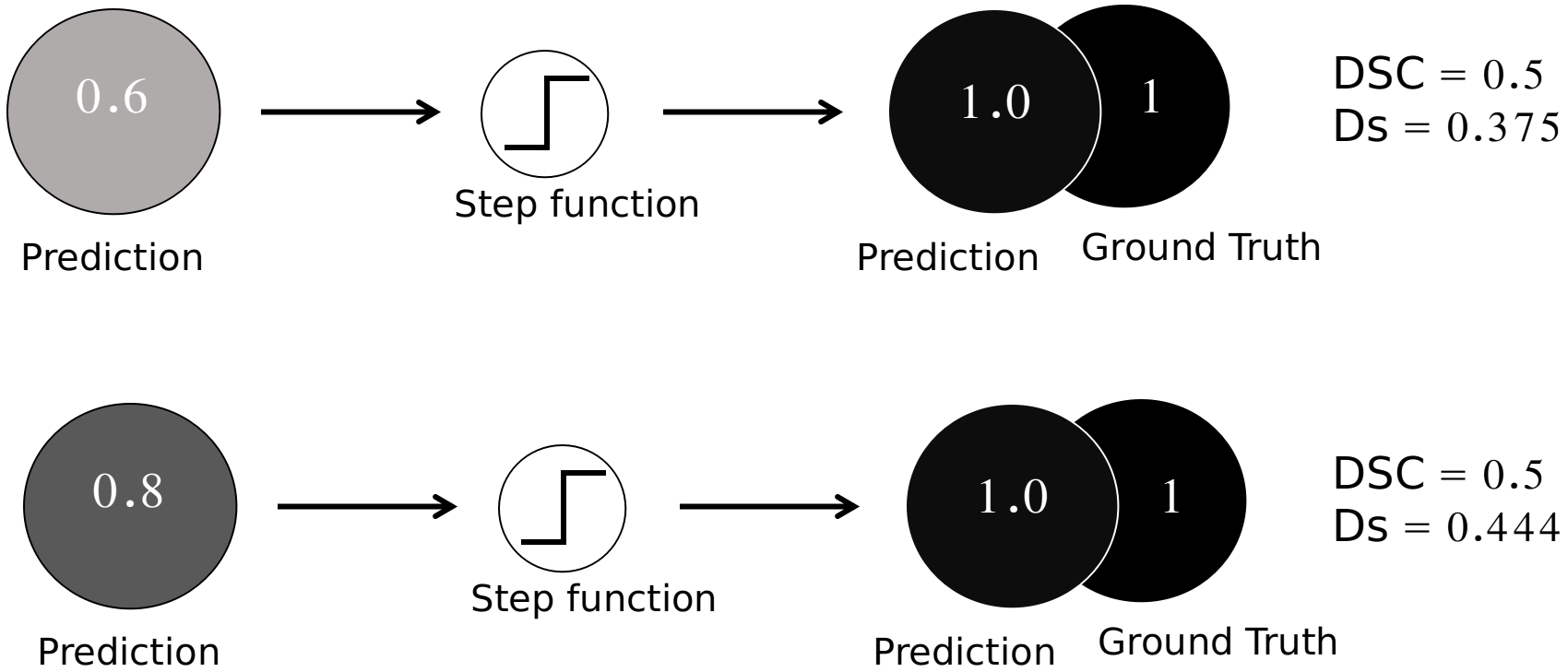
Figure 1: An example to illustrate the gap between DSC and Dice loss (Ds). Refer to text for more details.

Consider two overlapping disks, one is the ground truth segmentation with intensity value of $1$, and the other is the prediction with probabilities in the range of $[0,1]$. Assume the overlapping area between the ground truth and the prediction is half of the disk. To calculate DSC, the prediction map needs to be converted to binary through a Step function that uses $0.5$ as the threshold. In Fig. 1, two prediction maps are shown, with the across-the-board probabilities of $0.6$ and $0.8$, respectively. The upper case (prediction = $0.6$) has a Dice loss of $0.375$, and that for the lower case (prediction = $0.8$) is $0.444$. The discrete DSCs for them, however, are both $0.5$.

This example illustrates that decreases in the Dice loss do not necessarily lead to decreases (or even changes at all) in the values of DSC. This gap can pose serious difficulty in the network training procedure. Our approach to bridge the gap is through an activation function point of view, and the design will be presented in next section.

3 Remedy: Two-stage-multi-sized FCNs and a new activation function

As we mentioned in the previous section, when a single DSC-based FCN is utilized to segment lesions that have a vast variability in size, different types of segmentation biases may be generated. A combined remedy would be: 1) processing the images with sub-volumes of different sizes; and 2) treating large lesions and small lesions separately. While FCNs can handle images with arbitrary sizes, predetermined input size does affect the design of the network, especially the number of the layers. FCNs with small-sized input (we term them small-FCNs) and large-FCNs are more accurate for their respective sized lesions. With this in mind, the design of the fusion step should grant small-FCNs with more power to determine small lesions, while let large-FCNs be more authoritative about large lesions. This thought leads to the architecture of our two-stage-multi-sized FCNs model. In the first stage, we set up three FCN networks, for different sized neighborhoods, to best capture both large and small lesions. In stage two, the preliminary 3D lesions masks, which we term opinions, are first separated into small and large lesion groups, and then combined through nonlinear weighting schemes carried out by ensemble-nets.

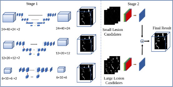
Figure 2: The overall structure of our model for lesion segmentation.

3.0.1 Stage 1: three different sized FCNs

In stage 1, we extract MR patches of three different sizes, and feed them into the corresponding FCNs. As each voxel may be covered by multiple patches, the prediction patches of each FCN are then sent back to the original image space to generate an overall probability map through averaging.

In order to fit our application and data, we made modifications to the 3D U-net [4] as follows. We keep the original design that two convolution layers are followed by one pooling/upsampling layer. The sizes of the convolution filters are set to $3\times 3\times 3$ except for the bottom layer of the U shape, in which the filter sizes are set to $1\times 1\times 1$. Every convolution layer is padded to maintain the same spatial dimension. The number of layers is reduced from 3D U-net as our input dimensions are smaller. The modified 3D U-net-like FCNs are shown in Fig. 2 Stage 1.

3.0.2 Stage 2: ensemble of preliminary opinions

Three opinions are generated in Stage 1 for each MR image. Stage 2 is to merge them to produce an overall lesion segmentation. As we described in a previous section, each FCN in the first stage is more trustworthy in processing one specific type of lesions, i.e., small-FCNs generate more reliable segmentations for small lesions, while large-FCNs performs better on large lesions. To take the advantage of this fact, we separate the estimated lesions within each prediction map into small and large lesion groups and send them into two different ensemble nets for fusion. In this work, an empirical threshold of $1000$-voxel has been used to decide the category (small or large) for any given lesion (a 3D connected component).

3.0.3 Ensemble net

The functionality of the two ensemble nets can both be expressed as

$$\min_{w_{1},w_{2},w_{3}}D(\mathbf{y},f(w_{1}\mathbf{x_{1}}+w_{2}\mathbf{x_{2}}+w_{3}\mathbf{x_{3}}))$$ (3)

where $\mathbf{x_{1}}$, $\mathbf{x_{2}}$, $\mathbf{x_{3}}$ are the contributing $opinion$s from the three FCNs; $\mathbf{y}$ is the corresponding ground truth. $D(\cdot,\cdot)$ measures the distance between the combined opinion and the ground-truth. With different approaches for the combination, $f(\mathbf{x})$ can be formulated as either a linear or non-linear function that maps $\mathbf{x}$ to the probability space. As we explained before, the combining weights $w_{1}$, $w_{2}$ and $w_{3}$ should be individualized for small and large lesion groups, respectively. Learning such weights can also be conducted through neural networks. In both small and large lesion groups, if we concatenate the three opinions as three channels, and treat $w_{1}$, $w_{2}$ and $w_{3}$ as a filter of size $(1,1,1,3)$, we can build an ensemble net of one convolution layer to learn the optimal weights in Eqn. 3. The $f(\mathbf{x})$ function in Eqn. 3 works as the activation function for this ensemble net.

We use Dice loss as the objective function of our ensemble-nets, to produce probability maps that match the ground-truth binary segmentations. As we explained in section 2, a theoretical gap exists between the DSC and Dice loss. An observation is that activation functions that are closer to the Step function would be able to produce better approximations for the DSC, at least from the numerical point-of-view. In this regard, an “ideal” activation function should be differentiable and relatively steep around $0.5$. Meanwhile, a reasonable capture or support range should be allowed to avoid vanishing gradients.

In FCN solutions for binary segmentation, the Sigmoid function is a commonly used activation function. In our ensemble nets, however, the inputs to the function $f(\mathbf{x})$ have a particular range of $[0,1]$, and a steeper function, if tailored to the inputs, would be preferred over the Sigmoid in producing more accurate DSC approximations. With these two considerations, we propose a new activation function for our ensemble nets:

$$H(x)=\begin{cases}1\quad\phantom{\infty}\text{if}\,\,x>1\\ 0\quad\phantom{\infty}\text{if}\,\,x<0\\ x+\frac{1}{2\pi}\sin(2\pi x-\pi)\quad\phantom{\infty}\text{if}\,\,0\leq x\leq 1\end{cases}$$ (4)

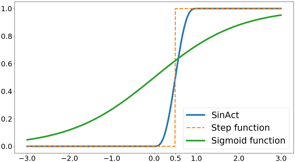
Figure 3: Comparison of Step, SinAct and Sigmoid functions.

We term $H(x)$ SinAct function. Fig. 3 shows a comparison of the Step, SinAct and Sigmoid functions. Compared with Sigmoid, the SinAct is steeper between $0$ and $1$. As we usually use $0.5$ as the threshold to convert probability maps into binary results, being steep around $0.5$ is a desired property. Another merit of SinAct function is that it evaluates to $0$ when the input is equal or smaller than $0$, and produces $1$ when the input is equal to $1$ and beyond. By contrast, the Sigmoid can approach infinitely close to $0$ and $1$, but would never reach the exact values.

4 Experiments

Data The MR data used in this paper were obtained from the White Matter Hyperintensities (WMH) Segmentation Challenge at MICCAI 2017 (http://wmh.isi.uu.nl/). The training set of this challenge contains images of 60 subjects acquired at three sites [7]. For each subject, a pair of aligned T1-weighted and Fluid-attenuated inversion recovery (FLAIR) images are available. Several pre-processing steps are conducted on all image pairs. First, skulls are removed from both T1 and FLAIR images using FSL/BET tool. Second, the intensities of all images are individually normalized to the range of $[0,1]$. 3D patches (sub-volumes) are extracted from the intensity-normalized brains using sliding windows. The patch sizes are set to $6\times 10\times 6$, $12\times 20\times 12$ and $24\times 40\times 24$ respectively, and the strides are half of the corresponding patch sizes. T1 and FLAIR patches from the same areas are concatenated as two channels and fed into the FCNs in Stage 1.

Implementation Details With the sliding windows of the aforementioned patch sizes, we found the extracted patches containing no lesion at all (“empty patches”) greatly outnumbered those with lesions inside. This would create a serious data imbalance in the training if we would use all the patches. To tackle this issue, we kept all the lesion patches, but only randomly picked an equal number of empty patches.

The three FCNs in Stage 1 are developed under Keras. ReLu is used as the activation function for all layers except the last one, where softmax is utilized to produce the final prediction. Dice loss is used as the network objective function and ADAM is adopted as the optimization method. The learning rate is set to $5\mathrm{e}{-6}$, and it reduces $50\%$ every 10 epochs. In total, each FCN is trained for 30 epochs. In Stage 2, lesions are separated into two groups, small and large lesions, and FCN ensembles are carried out within the individual groups. Volume size of $1000$ voxels has been used as a hard threshold to determine the category for each 3D connected component. For the training subjects, the separation is based on their corresponding ground-truth, which means the component on the probability maps is assigned as a large lesion candidate if the corresponding groud truth component is larger than $1000$ voxels. In the testing stage, a threshold of $0.5$ is applied on the prediction probability map to produce a binary component first, then the map is assigned as either small or large based on the same threshold. To train our ensemble net, all three parameters in Eqn. 3 are initialized to $1/3$. Each ensemble net is trained for $10$ epochs.

Our experiment is carried out based on the training set of the WMH Segmentation Challenge through Monte Carlo cross-validation. $54$ of the $60$ subjects are randomly selected for training and the rest $6$ subjects are used for testing. The whole experiments are repeated $5$ times. The results are presented in next section.

4.1 Experimental results

Evaluations of the individual components and overall network are carried out based on five performance metrics: DSC, Hausdorff distance (HD, 95th percentile), Average volume difference (AVD, in percentage), Sensitivity for individual lesions (Detection, in percentage) and F-1 score for individual lesions. The evaluation code was provided by the Challenge organizers, available under the Challenge website.

The final segmentation results are shown in Table 1. FCNs with fixed input sizes are the baseline models, and we take ensemble-nets through majority vote and Sigmoid as the competing ensemble solutions. Our SinAct-based ensemble net outperforms all other models in every evaluation metric except detection. In detection, FCNs with the smallest patch size of $6\times 10\times 6$ achieve the highest score, but they perform the worst in all other metrics, in part because of high false positive (type I) errors. Compared with vote and Sigmoid, our SinAct-based ensemble-net solution achieves higher accuracy (measured by DSC) and consistency (measured by HD and AVD) at the same time.

Table 1: Segmentation results on all lesions.

		Results
FCN	Ensemble	Dice	HD	AVD	Detection	F1
$6\times 10\times 6$		77.74	17.82	21.72	81.83	57.41
$12\times 20\times 12$		79.78	4.65	19.28	72.43	69.91
$24\times 40\times 24$		80.39	3.95	18.43	73.55	71.03
3 FCNs	Vote	81.03	3.95	18.43	73.55	71.03
3 FCNs	Sigmoid	80.96	4.61	19.90	80.24	68.13
3 FCNs	SinAct	81.26	2.58	17.54	73.70	71.65

Table 2: Model performance on small and large lesions separately.

			Results
FCN	Lesion Size	Ensemble	Dice	HD	AVD	Detection	F1
$6\times 10\times 6$	Small		59.30	18.06	47.87	80.79	55.85
$12\times 20\times 12$	Small		60.90	10.24	29.55	70.36	67.39
$24\times 40\times 24$	Small		61.20	9.35	29.67	64.22	66.04
3 FCNs	Small	Vote	63.64	9.63	28.69	71.93	69.52
3 FCNs	Small	Sigmoid	65.07	11.51	34.42	78.98	64.74
3 FCNs	Small	SinAct	65.80	8.00	26.52	72.47	70.34
$6\times 10\times 6$	Large		85.59	7.08	15.33	98.89	90.02
$12\times 20\times 12$	Large		84.92	6.40	14.10	77.87	66.54
$24\times 40\times 24$	Large		85.13	6.81	12.99	69.39	64.22
3 FCNs	Large	Vote	85.32	8.23	14.05	76.31	68.19
3 FCNs	Large	Sigmoid	86.87	5.81	12.58	88.59	84.66
3 FCNs	Large	SinAct	86.69	5.87	12.33	86.84	76.84

Table 2 provides evaluations of the models on small and large lesions separately. For both small and large lesion groups, almost all ensemble nets outperform the fixed-sized FCNs in DSC, which to certain extent validates our design of combining multi-sized FCNs. As our SinAct function provides more accurate DSC approximations at voxels with uncertain labels, it improves the membership decision most significantly at the boundary voxels. Among the three ensemble-nets, our SinAct net performs the best, in all metrics, for small lesions. For large lesions, SinAct is still better than vote, but achieves comparable performance with the Sigmoid. This disparity can be explained by the fact that boundary voxels account for high percentage for small lesions, but not so for large lesions. All in all, FCNs and the new activation function are shown to be effective in improving MS lesions segmentations from MRIs.

5 Conclusions

In this paper, we propose a two-stage-multi-sized FCNs strategy to enhance the segmentation of MS white matter lesions in MR images. The design is based on the rational that different sized lesions are best captured with appropriate sized FCNs. Ensemble-nets are constructed to combine the results from the FCNs, where SinAct, a new activation function, is adopted to improve the segmentation accuracy measured by DSC. Experiments show the effectiveness of both design approaches. Exploring more activation functions is the directions of our future efforts. We are also interested in applying the proposed strategy to other neuroimage analysis problems.

References

- [1] Anbeek, P., et al.: Automatic segmentation of different-sized white matter lesions by voxel probability estimation. Medical image analysis 8(3), 205–215 (2004)
- [2] Chen, Y., Shi, B., Wang, Z., Sun, T., Smith, C.D., Liu, J.: Accurate and consistent hippocampus segmentation through convolutional LSTM and view ensemble. In: Machine Learning in Medical Imaging. pp. 88–96 (2017)
- [3] Chen, Y., Shi, B., Wang, Z., Zhang, P., Smith, C.D., Liu, J.: Hippocampus segmentation through multi-view ensemble convnets. In: 14th IEEE, ISBI 2017. pp. 192–196 (2017)
- [4] Çiçek, Ö., et al.: 3d u-net: Learning dense volumetric segmentation from sparse annotation. In: MICCAI. pp. 424–432. Springer (2016)
- [5] Drozdzal, M., et al.: The importance of skip connections in biomedical image segmentation. In: Deep Learning and Data Labeling for Medical Applications, pp. 179–187. Springer (2016)
- [6] Ekanayake, J., et al.: Generalised wasserstein dice score for imbalanced multi-class segmentation using holistic convolutional networks. In: Third International Workshop, BrainLes, MICCAI 2017
- [7] Li, H., et al.: Fully convolutional network ensembles for white matter hyperintensities segmentation in mr images. arXiv preprint arXiv:1802.05203 (2018)
- [8] Liu, J., Smith, C.D., Chebrolu, H.: Automatic multiple sclerosis detection based on integrated square estimation. In: IEEE, CVPR Workshops, 20-25 June, 2009. pp. 31–38 (2009)
- [9] Long, J., et al.: Fully convolutional networks for semantic segmentation. In: Proceedings of CVPR. pp. 3431–3440 (2015)
- [10] Milletari, F., et al.: V-net: Fully convolutional neural networks for volumetric medical image segmentation. In: 3D Vision (3DV). pp. 565–571. IEEE (2016)
- [11] Ronneberger, O., Fischer, P., Brox, T.: U-net: Convolutional networks for biomedical image segmentation. In: MICCAI. pp. 234–241. Springer (2015)
- [12] Souplet, J.C., et al.: An automatic segmentation of t2-flair multiple sclerosis lesions. In: The MIDAS Journal-MS Lesion Segmentation (MICCAI 2008 Workshop). Citeseer (2008)
- [13] Sudre, C.H., et al.: Generalised dice overlap as a deep learning loss function for highly unbalanced segmentations. In: Deep Learning in Medical Image Analysis and Multimodal Learning for Clinical Decision Support, pp. 240–248. Springer (2017)
- [14] Warfield, S., Tomas-Fernandez, X.: Lesion segmentation. In: Toga, A.W. (ed.) Brain Mapping, pp. 323 – 332. Academic Press, Waltham (2015)