Self-Paced Learning with
Adaptive Deep Visual Embeddings

Abstract

Selecting the most appropriate data examples to present a deep neural network (DNN) at different stages of training is an unsolved challenge. Though practitioners typically ignore this problem, a non-trivial data scheduling method may result in a significant improvement in both convergence and generalization performance. In this paper, we introduce Self-Paced Learning with Adaptive Deep Visual Embeddings (SPL-ADVisE), a novel end-to-end training protocol that unites self-paced learning (SPL) and deep metric learning (DML). We leverage the Magnet Loss to train an embedding convolutional neural network (CNN) to learn a salient representation space. The student CNN classifier dynamically selects similar instance-level training examples to form a mini-batch, where the easiness from the cross-entropy loss and the true diverseness of examples from the learned metric space serve as sample importance priors. To demonstrate the effectiveness of SPL-ADVisE, we use deep CNN architectures for the task of supervised image classification on several coarse- and fine-grained visual recognition datasets. Results show that, across all datasets, the proposed method converges faster and reaches a higher final accuracy than other SPL variants, particularly on fine-grained classes.

1 Introduction

The standard method for training deep neural networks (DNNs) is stochastic gradient descent (SGD), which employs backpropagation to compute gradients. It typically relies on fixed-size mini-batches of random samples drawn from a finite dataset. However, the contribution of each sample during model training varies across training iterations and configurations of the model’s parameters (Lapedriza et al., 2013). This raises the importance of data scheduling for training DNNs; that is, searching for an optimal ordering of training examples that are presented to the model. Previous studies on curriculum learning (CL) (Bengio et al., 2009) show that organizing training samples based on the ascending order of difficulty can be favourable for model training. However, in CL, the curriculum remains fixed over the iterations and is determined without any knowledge or introspection of the model’s learning. Self-paced learning (Kumar et al., 2010) presents a method for dynamically generating a curriculum by biasing samples based on their easiness under the current model parameters. This can lead to a highly imbalanced selection of samples, i.e. very few instances of some classes are chosen, which negatively affects the training process due to overfitting. Loshchilov and Hutter (2015) propose a simple batch selection strategy based on the loss values of training data for speeding up neural network training. However, the approach is computationally expensive and the results are inconclusive, as it achieves high performance on MNIST, but fails on CIFAR-10. Their work reveals that selecting the examples to present to a DNN is non-trivial, yet the strategy of uniformly sampling the training data set is not necessarily the optimal choice.

Jiang et al. (2014) show that partitioning the data into groups with respect to diversity and easiness in their self-paced learning with diversity (SPLD) framework, can have a substantial effect on training. Rather than constraining the model to limited groups, they propose to spread the sample selection as wide as possible to obtain diverse samples of similar easiness. However, their use of $K$-Means and Spectral Clustering to partition the data into groups can lead to sub-optimal clustering results when learning non-linear feature representations. Therefore, learning an appropriate metric by which to capture similarity among arbitrary groups of data is of great practical importance. Deep metric learning (DML) approaches have recently attracted considerable attention and have been the focus of numerous studies (Bell and Bala, 2015; Schroff et al., 2015). The most common methods are supervised, where a feature space in which distance corresponds to class similarity is obtained. The Magnet Loss (Rippel et al., 2016) presents state-of-the-art performance on fine-grained classification tasks. Song et al. (2017) show that it achieves state-of-the-art on clustering and retrieval tasks.

This paper makes two key contributions toward scheduling data examples in the mini-batch setting: (1) We propose a general sample selection framework called Self-Paced Learning with Adaptive Deep Visual Embeddings (SPL-ADVisE) that is independent of model architecture or objective, and learns when to introduce certain samples to the DNN during training. (2) To our knowledge, we are the first to leverage metric learning to improve SPL. We exploit a new type of knowledge —similar instance-level samples are discovered through an embedding network trained by DML concurrently with the self-paced learner.

2 Related Work

Learning Small and Easy. The perspective of “starting small and easy” for structuring the learning regimen of neural networks dates back decades to (Elman, 1993). Recent studies show that selecting a subset of good samples for training a classifier can lead to better results than using all the samples (Lee and Grauman, 2011; Lapedriza et al., 2013). Pioneering work in this direction is CL (Bengio et al., 2009), which introduced a heuristic measure of easiness to determine the selection of samples from the training data. By comparison, SPL (Kumar et al., 2010) quantifies the easiness by the current sample loss. The training instances with loss values larger than a threshold, $\lambda$, are neglected during training and $\lambda$ dynamically increases in the training process to include more complex samples, until all training instances are considered. Previous studies prove that CL and SPL strategies are instrumental in avoiding bad local minima and improving generalization (Khan et al., 2011; Gülçehre and Bengio, 2016; Peng, 2017). This theory has been widely applied to various problems, including visual tracking (Huang et al., 2017), medical imaging analysis (Li et al., 2017), and person re-identification (Zhou et al., 2018). In CL, the increasing entropy theory shows that a curriculum should progressively increase the diversity of training examples during learning. An effective SPL strategy should generate a curriculum that includes easy and diverse examples that are sufficiently dissimilar from what a DNN has already learned. In SPLD (Jiang et al., 2014), training data are pre-clustered in order to balance the selection of the easiest samples with a sufficient inter-cluster diversity. However, the clusters and the feature space are fixed: they do not depend on the current self-paced training iteration. Adaptation of this method to a deep learning scenario, where the feature space changes during learning, is non-trivial. Our self-paced sample selection framework targets a similar goal but obtains diversity of samples through a DML approach to adaptively sculpt a representation space by autonomously identifying and respecting intra-class variation and inter-class similarity.

Learning the Metric Space. Deep metric learning has gained much popularity in recent years, along with the success of deep learning. The objective of DML is to learn a distance metric consistent with a given set of constraints, which usually aim to minimize the distances between pairs of data points from the same class and maximize the distances between pairs of data points from different classes. DML approaches have shown promising results on various tasks, such as zero-shot learning (Frome et al., 2013), face recognition (Schroff et al., 2015), and feature matching (Choy et al., 2016). DML can also be used for challenging, extreme classification settings, where the number of classes is very large and the number of examples per class becomes scarce. Most DML methods define the loss in terms of pairs (Song et al., 2016), triplets (Wang et al., 2017) or $n$-pair tuples (Sohn, 2016) inside the training mini-batch. These methods require a separate data preparation stage, which has a very expensive time and space cost. Also, they do not take the global structure of the embedding space into consideration, which can result in reduced clustering. An alternative is the Magnet Loss (Rippel et al., 2016), DML via Facility Location (Song et al., 2017), and Class-Conditional Metric Learning (CCML) (Im and Taylor, 2016), which do not require the training data to be preprocessed in rigid paired format and are aware of the global structure of the embedding space. Our work employs the Magnet Loss to learn a representation space, where we compute centroids on the raw features and then update the learned representation continuously.

To our knowledge, the concept of employing DML for SPL-based DNN training has not been investigated. Effectively, a deep CNN trained by the Magnet Loss learns a representation in which a clustering of that space represents the diversity of the data. A student model exploits this space by forming dynamic mini-batches that select samples based on true diverseness defined by that clustering and easiness defined by the student’s current loss. Our architecture combines the strength of adaptive sampling, the efficiency of mini-batch online learning, and the flexibility of representation learning to form an effective self-paced strategy in an end-to-end DNN training protocol.

3 Proposed Method

The Self-Paced Learning with Adaptive Deep Visual Embeddings (SPL-ADVisE) framework consists of dual complementary DNNs. An embedding DNN learns a salient representation space, then transfers its knowledge to the self-paced selection strategy for training the second DNN, called the student. In this work, but without loss of generality, we focus on training deep CNNs for the task of supervised image classification. More specifically, an embedding CNN is trained alongside the student CNN of ultimate interest (Figure 1). In this framework, we want to form mini-batches using the easiness and true diverseness as sample importance priors for the selection of training samples. Given that we are learning the representation space adaptively alongside the student as training progresses, this has negligible computational cost compared to the actual training of the student CNN (see Section 4).

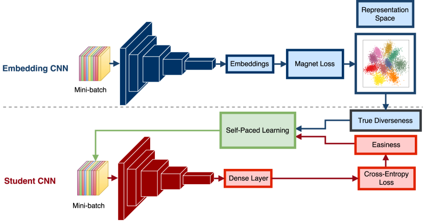
Figure 1: The SPL-ADVisE framework, consisting of an embedding CNN that learns a representation for the student CNN to create a self-paced strategy based on easiness and true diverseness as sample importance priors.

3.1 Embedding CNN

Though there are many possible DML frameworks from which to choose, we adopt the Magnet Loss (Rippel et al., 2016) because of its strong empirical gains relative to popular baselines such as the margin-based Triplet loss and softmax regression. Assuming we have a training set with $N$ input-label pairs $\mathcal{D}=\{\mathbf{x}_{n},y_{n}\}_{n=1}^{N}$, the Magnet Loss learns the distribution of distances for each example, to $K$ clusters assigned for each class, $c$, denoted as $\{\mathcal{I}_{k}^{c}\}_{k=1}^{K}\ \forall\ C$ classes. The mapping of inputs to representation space are parameterized by $\textbf{f}(\cdot;\Theta)$, where their representations are defined as $\textbf{r}_{n}=\{\textbf{f}(x_{n};\Theta)\}_{n=1}^{N}$. The cluster assignments are then repositioned using an intermediate $K$-Means++ clustering (Arthur and Vassilvitskii, 2007). Therefore, for each class $c$, we have,

$$\{\mathcal{I}_{k}^{c}\}_{k=1}^{K} =\mathop{\text{argmin}}\limits_{I_{1}^{c},\ldots,I_{K}^{c}}\sum_{k=1}^{K}\sum_{r\in I_{k}^{c}}\|\textbf{r}-\mu_{k}^{c}\|_{2}^{2},$$

$$\mu_{k}^{c} =\frac{1}{\|I_{k}^{c}\|}\sum_{\textbf{r}\in I_{k}^{c}}\textbf{r}.$$

The class and assigned cluster centre of r are defined as $C(\textbf{r})$ and $\mu_{k}^{c}$, respectively. The optimized indices are represented by $\mathcal{I}$, while the indices that are the variates of the optimization are represented by $I$. In the training procedure, the embedding CNN constructs mini-batches with neighbourhood sampling, where we sample a local neighbourhood at each iteration.

First, a seed cluster is sampled $I_{1}\sim p_{\mathcal{I}}(\cdot)$, and then the nearest $M-1$ imposter clusters $\{I_{m}\}_{m=2}^{M}$ are fetched for $I_{1}$, where $M$ number of mini-batch clusters is chosen to be $M\leq K$. The objective of learning the metric is to ensure that nearest neighbours that belong to the same class are clustered together, while imposters are moved away by a large margin. Imposter clusters are considered to be groups of points that have nearest neighbours with different labels, i.e. clusters of examples from different classes. Finally, $B$ training instances $\{x_{b}^{m}\}_{b=1}^{B}\sim p_{I_{m}}(\cdot)$ are uniformly sampled for each cluster $\{I_{m}\}_{m=1}^{M}$. The $p_{\mathcal{I}}(\cdot)$ and $p_{I_{m}}(\cdot)$ choices enable us to adapt to the current distributions of each example in the representation space. Therefore, during training, contested neighbourhoods with large cluster overlap can be targeted and reprehended.

The losses of each example are stored and the average loss $\mathcal{L}$ is computed during training. Hence, the stochastic approximation of the Magnet Loss can be more formally described as:

$$\mathcal{L}(\Theta)=\frac{1}{MB}\sum_{m=1}^{M}\sum_{b=1}^{B}\Bigg{\{}-\log\bigg{(}\frac{e^{-\frac{1}{2\sigma^{2}}\|\textbf{r}_{b}^{m}-\mu_{m}\|_{2}^{2}-\alpha}}{\sum_{\mu:C(\mu)\neq C(\textbf{r}_{b})}e^{-\frac{1}{2\sigma^{2}}\|\textbf{r}_{b}^{m}-\mu\|_{2}^{2}}}\bigg{)}\Bigg{\}}_{+},$$ (1)

where $\{\cdot\}_{+}$ is the hinge function, $\alpha\in\mathbb{R}$ is the desired separation parameter, the cluster mean is $\mu_{m}=\frac{1}{B}\sum_{b=1}^{B}\textbf{r}_{b}^{m}$, and the variance of all samples from their respective centers is given by $\sigma=\frac{1}{MB-1}\sum_{m-1}^{M}\sum_{b=1}^{B}\|\textbf{r}_{b}^{m}-\mu_{m}\|_{2}^{2}$. A K-Means cluster index is used to capture the distribution of $c$ in the embedding space for all classes $C$. A cluster refresh interval $R$ is used to reinitialize each index using K-Means++. We pause the embedding CNN training and perform forward passes of all inputs to get the representations $\textbf{r}_{n}$ to be indexed. The cost of K-Means++ clustering is negligible because the cluster index is not refreshed frequently and we only run forward passes of the inputs (Rippel et al., 2016). The process for training the embedding CNN is provided in Algorithm 1.

Input : $\mathcal{D}$ (training data), $B$ (per-cluster batch size), $M$ (mini-batch clusters),

$C$ (classes), $E$ (embedding CNN iterations), $R$ (cluster refresh interval)

Output : A representation space $\mathcal{D}_{1}^{1},\ldots,\mathcal{D}_{K}^{C}$.

1

2Extract initial representations $\textbf{r}_{n}=\{\textbf{f}(x_{n};\Theta)\}_{n=1}^{N}$.

3 Initialize cluster assignments $\{\mathcal{I}_{k}^{c}\}_{k=1}^{K}\ \forall\ C$ using K-Means++.

4 for each iteration $\{e=1,\ldots,E\}$ do

5       Sample seed cluster $I_{1}\sim p_{\mathcal{I}}(\cdot)$.

6       Fetch impostor clusters $\{I_{m}\}_{m=2}^{M}$ for $I_{1}$.

7       Uniformly sample $\{x_{b}^{m}\}_{b=1}^{B}\sim p_{I_{m}}(\cdot)$ for each $m$, to form mini-batch.

8       Extract mini-batch representations $\textbf{r}_{b}^{m}=\{\textbf{f}(x_{b}^{m};\Theta)\}_{b=1}^{B}$ for each $m$.

9       Compute $\mathcal{L}(\Theta)$ as in Eq. 1.

10       if e == R then

11             Repeat steps $1-2$.

12            

13       end if

14      

15 end for

return $\mathcal{D}_{1}^{1},\ldots,\mathcal{D}_{K}^{C}$

Algorithm 1 Train Embedding CNN with Magnet Loss.

3.2 SPL-ADVisE Framework

The aim of SPL-ADVisE can be formally described as follows. Let us assume that a training set $\mathcal{D}$ consisting of $N$ examples, $\mathcal{D}=\{\mathbf{x}_{n}\}_{n=1}^{N}$ is grouped into $K$ clusters for $C$ classes using Algorithm 1. Therefore, we have $\{\mathcal{D}^{k}\}_{k=1}^{K}$, where $\mathcal{D}^{k}$ corresponds to the $k^{th}$ cluster, $n_{k}$ is the corresponding number of examples in that cluster and $\sum_{k=1}^{K}n_{k}=N$. The weight vector is denoted accordingly as $\{\mathcal{W}^{k}\}_{k=1}^{K}$, where $\mathcal{W}^{k}=(\mathcal{W}_{1}^{k},\ldots,\mathcal{W}_{n_{k}}^{k})^{T}\in[0,1]^{n_{k}}$. Non-zero weights of $\mathcal{W}$ are assigned to samples that the student model considers “easy” and non-zero elements are distributed across more clusters to increase diversity. Thus, in the SPL-ADVisE framework, we optimize the following objective:

$$\min_{\theta,\mathcal{W}}\mathbb{E}(\theta,\mathcal{W};\lambda,\gamma) =\sum_{i=1}^{N}\mathcal{W}_{i}\mathcal{L}_{ce}(y_{i},f(x_{i},\theta))-\lambda\sum_{i=1}^{N}\mathcal{W}_{i}-\gamma\|\mathcal{W}\|_{2,1},\ \text{s.t}\ \mathcal{W}\in[0,1]^{N},$$ (2)

where $\mathcal{L}_{ce}$ is the cross-entropy loss, and $\lambda$, $\gamma$ are the two pacing parameters for sampling based on easiness and the true diverseness as sample importance priors, respectively. The negative $l_{1}$-norm: $-\|\mathcal{W}\|_{1}$ is used to select easy samples over hard samples, as seen in conventional SPL. The negative $l_{2,1}$-norm inherited from the original SPLD algorithm is used to disperse non-zero elements of $\mathcal{W}$ across a large number of clusters to obtain a diverse selection of training samples. Therefore, the diversity term $-\|\mathcal{W}\|_{2,1}$ is defined as $-\sum_{k=1}^{K}\|\mathcal{W}^{k}\|_{2}$. The student CNN receives the up-to-date model parameters $\theta$, a diverse cluster of samples, $\lambda$, $\gamma$ and outputs the optimal $\mathcal{W}$ of $\displaystyle\min_{\mathcal{W}}\mathbb{E}(\theta,\mathcal{W};\lambda,\gamma)$ for extracting the global optimum of this optimization problem. The detailed algorithm to train the student CNN with SPL-ADVisE is presented in Algorithm 2.

Input : $\mathcal{D}$ (training data), $E^{\prime}$ (student CNN iterations), $\{\beta_{1},\beta_{2}\}$ (pace adaptation parameters)

Output : The model parameters $\theta$.

1 Initialize $\mathcal{W}^{*},\lambda,\gamma$ ;

2

3Update embedding CNN using Algorithm 1, in parallel with steps 3-16.

4 for each iteration $\{{e^{\prime}=1,\ldots,E^{\prime}}\}$ do

5      

6      $\theta^{*}=\mathop{\text{argmin}}_{\theta}\mathbb{E}(\theta,\mathcal{W}^{*};\lambda,\gamma)$. // Train Student CNN model.

7       // Solve $\min_{\mathcal{W}}\mathbb{E}(\theta,\mathcal{W};\lambda,\gamma)$

8       Get clusters $\{D^{k}\}_{k=1}^{K}$ from the embedding CNN.

9       for each cluster $\{k=1,\ldots,K\}$ do

10             Sort training samples in increasing order of $\mathcal{L}$.

11             Represent the labels of $D^{k}\ \text{as}\ \{y_{1}^{k},\ldots,y_{n_{k}}^{k}\}$ and weights as $\{\mathcal{W}_{1}^{k},\ldots,\mathcal{W}_{n_{k}}^{k}\}$.

12             for each sample $i=\{1,\ldots,n_{k}\}$ do

13                   if $\mathcal{L}_{ce}(y_{i}^{k},f(x_{i}^{k},\theta^{*}))<(\lambda+\gamma\frac{1}{\sqrt{i}+\sqrt{i-1}})$ then  $\mathcal{W}_{i}^{k}=1$ ;

14                   else  $\mathcal{W}_{i}^{k}=0$ ;

15                  

16             end for

17            

18       end for

19      $\mathcal{W}^{*}$ = $\mathcal{W}$;    $\theta=\theta^{*}$;

20       $\lambda\leftarrow\beta_{1}\lambda$;    $\gamma\leftarrow\beta_{2}\lambda$; // Update pace.

21      

22 end for

Algorithm 2 Train Student CNN with SPL-ADVisE.

For any $\theta$, we show how we can solve for the global optimum to $\displaystyle\min_{\mathcal{W}}\mathbb{E}(\theta,\mathcal{W})$ in linearithmic time. The alternative search strategy outlined in Algorithm 2 can be easily employed to solve Eq. 2. Step 11 of Algorithm 2 generalizes the three conditions for selecting samples in terms of both the easiness and the true diverseness. (1) During training, “easy” samples are selected when $\mathcal{L}_{ce}(y_{i}^{k},f(x_{i}^{k},\theta))<\lambda$, thus $\mathcal{W}_{i}=1$. Here, SPL-ADVisE effectively becomes SPL because $\gamma=0$, hence the smallest losses from a single cluster are assigned weights. (2) Otherwise in Step 12, $\mathcal{W}_{i}=0$ if the $\mathcal{L}_{ce}(y_{i}^{k},f(x_{i}^{k},\theta))>\lambda+\gamma$, which represents the “hard” samples with higher losses. (3) We select other samples by ranking a sample with respect to its loss value within its cluster, denoted by $i$. Then, we compare the losses to a threshold $\lambda+\gamma\frac{1}{\sqrt{i}+\sqrt{i-1}}$. Step 11 penalizes samples repeatedly selected from the same cluster, seeing as this threshold decreases as the sample’s rank $i$ grows. The $\lambda$ and $\gamma$ pace parameters are updated at the end of training iteration (Step 16). These two pacing parameters are empirically found by the statistics collected from ranked samples, which is more robust than by setting absolute values for SPL-ADVisE. This is because setting by absolute values can result in selecting too many or too few samples. Specifically, $\lambda$ and $\gamma$ are set according to the ranked samples, and then absolute values are calculated accordingly. The two pace adaptation parameters $\{\beta_{1},\beta_{2}\}$ in Algorithm 2 are factors that are used to introduce increasingly hard and diverse samples from one iteration to the next.

Compared to the original loss function $\mathcal{L}_{ce}$, it is evident that there is a suppressing effect of the latent SPL loss function on large losses (Meng et al., 2017). In SPL-ADVisE, we embed the true diverseness prior, in addition to easiness. We can encode these two priors into the latent variables as a regularizer and avoid unreasonable local minima. This allows us to select high-confidence samples that are dispersed across the input space, incrementally learning meaningful knowledge through robust guidance. As a result, we produce a training scheme that exploits a diverse curriculum consisting of easy samples from multiple clusters within a learned representation space.

4 Experiments

All experiments were conducted using the PyTorch framework, while leveraging containerized multi-GPU training on NVIDIA P100 Pascal GPUs through Docker. We compared our SPL-ADVisE framework against the original SPLD algorithm and Random Sampling on FashionMNIST, SVHN, CIFAR-10 and CIFAR-100. We tried 5 different combinations of $\{\beta_{1},\beta_{2}\}$ for SPL-ADVisE, and determined that $\beta_{1}=0.1$ and $\beta_{2}=0.1$ provided the best combination with the smallest error rate. The embedding CNN is trained in parallel with the student CNN. The computational requirement of training the embedding CNN is mitigated by leveraging multiprocessing for parallel computing to share data between processes locally using arrays and values. In our experiments, we mainly compare convergence in terms of number of mini-batches required to achieve a comparable state-of-the-art test performance. We also visualize the original high-dimensional representations using t-SNE (van der Maaten and Hinton, 2008), where the different colours correspond to different classes and the values to density estimates.

FashionMNIST. In the experiments for FashionMNIST (Xiao et al., 2017), we extract feature embeddings from a LeNet (LeCun et al., 2001) as the embedding CNN, and learn a representation space using the Magnet Loss. The fully-connected layer of the LeNet is replaced with an embedding layer for compacting the distribution of the learned features for feature similarity comparison using the Magnet Loss. The student CNN (classifier) was a ResNet-18 (He et al., 2016), which we then trained with our SPL-ADVisE framework. The embedding CNN was trained with mini-batches of size 64 and optimized using Adam with a learning rate of 0.0001. The classifier is trained using SGD with Nesterov momentum of 0.9, weight decay of 0.0005, and a learning rate of 0.001. We performed data augmentation on the FashionMNIST training set with normalization, random horizontal flip, random vertical flip, random translation, random crop, and random rotation. As shown in Table 1, the SPL-ADVisE framework results in an increase in test accuracy by between 0.95 and 1.35 percentage points on FashionMNIST.

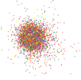
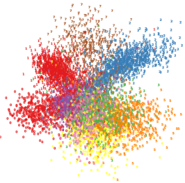
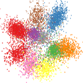
Figure 2: t-SNE visualizations of the SVHN representation space at different stages of training the embedding CNN. (a) Start of training. (b) 6000 mini-batch updates. (c) Final representation space.

SVHN. The Street View House Numbers (SVHN) dataset (Netzer et al., 2011) is a real-world image dataset with 630,420 RGB images of 32$\times$32 pixels in size, where each image consists of digits that are from one of ten different classes. The SVHN dataset is split into the training set, testing set, and extra set with 73,257, 26,032, and 531,131 images, respectively. The student CNN used to train on the SVHN dataset was a WideResNet with a fixed depth of 16, a fixed widening factor of 8, and dropout probability of 0.4. The SVHN training set and extra set were combined for a total of 604,388 images to train the student CNN for 65 epochs and no data augmentation scheme was applied. The student model was optimized using SGD with Nesterov momentum of 0.9, weight decay of 0.0005, and batch-size of 128. Our experiments revealed that VGG-16 (Simonyan and Zisserman, 2014) learned strong and rich feature representations, which yielded the best convergence on the Magnet Loss. Therefore, we treat the VGG-16 model as a feature extraction engine and use it for feature extraction from SVHN images, without any fine-tuning. The VGG-16 network is trained with randomly sampled mini-batches of size 64 and optimized using Adam at a learning rate of 0.0001. The learned feature representation space of the SVHN data is depicted in Figure 2. The results in Figure 3 show that SPL-ADVisE is able to converge faster to a higher test accuracy than Random Sampling and SPLD.

CIFAR-10. The CIFAR-10 dataset (Krizhevsky and Hinton, 2009) consists of 50,000 examples in the training set and 10,000 examples in the test set. Each example is a 32$\times$32 RGB image associated with a label from 10 classes. The CIFAR-10 training set was augmented with normalization, random horizontal flip, and random crop. We used VGG-16 as our embedding CNN and ResNet-18 as our classifier in the CIFAR-10 experiments. We chose ResNet-18 over other architectures because it is faster to train and achieves good performance on CIFAR-10. The embedding CNN was a VGG-16 setup similar to our SVHN experiments. The CIFAR-10 experiment followed the learning rate scheduler identical to that of the WideResNet (Zagoruyko and Komodakis, 2016) training scheme. The classifier is trained with batch sizes of 128, using SGD with a momentum of 0.9, weight decay of 0.0005, and a starting learning rate of 0.1 which is dropped by a factor of 0.1 at 60, 120 and 160 epochs. In our experiments, this would translate to 23,400, 46,800, and 62,400 mini-batch updates. Our CIFAR-10 experiments with the learning rate scheduler shows that SPL-ADVisE converges faster earlier on in training compared to SPLD and Random Sampling (Figure 3). As the learning rate drops by a factor of 0.1 at 23,400, 46,800, and 62,400 mini-batch updates, the classifier under the SPL-ADVisE training protocol improves test performance by 1.17 and 2.22 percentage points over SPLD and Random Sampling, respectively.

CIFAR-100. The CIFAR-100 dataset (Krizhevsky and Hinton, 2009) contains 100 classes and the same number of samples in the training/test set as CIFAR-10. We evaluated our SPL-ADVisE framework on CIFAR-100 with a WideResNet (student CNN) that has a fixed depth of 28, a fixed widening factor of 10, and dropout probability of 0.3. The embedding CNN was a VGG-16 setup similar to our SVHN and CIFAR-10 experiments. The optimizer and learning rate scheduler used for training the WideResNet was identical to the CIFAR-10 experiments. A data augmentation scheme was not applied on the CIFAR-100 dataset. The results in Figure 3 reveal that on CIFAR-100, there are noticeable gains in test performance over baseline methods. SPL-ADVisE was able to increase test accuracy by between 3.81 and 4.75 percentage points.

Method	FashionMNIST	SVHN*	CIFAR-10	CIFAR-100*
SPL-ADVisE	94.12 $\pm$ 0.11	97.68 $\pm$ 0.09	95.48 $\pm$ 0.16	79.17 $\pm$ 0.24
SPLD	93.17 $\pm$ 0.18	97.38 $\pm$ 0.06	94.31 $\pm$ 0.21	75.36 $\pm$ 0.30
Random Sampling	92.77 $\pm$ 0.14	97.41 $\pm$ 0.11	93.26 $\pm$ 0.12	74.42 $\pm$ 0.25

Table 1: Experimental results across all datasets (FashionMNIST, CIFAR-10, CIFAR-100, and SVHN) and sampling methods (SPL-ADVisE, SPLD, and Random Sampling). The test accuracy (%) results are averaged over 5 runs and “*” indicates that no data augmentation scheme was applied on the dataset.

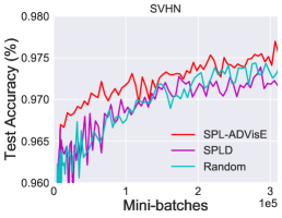
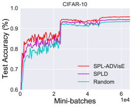
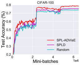
Figure 3: Averaged test curves of 5 independent runs on (a) SVHN, (b) CIFAR-10 with standard data augmentation, and (c) CIFAR-100. The solid line represents our SPL-ADVisE framework.

5 Discussion

We have shown that fusing a salient non-linear representation space with a dynamic learning strategy can help a DNN converge towards an optimal solution. A random curriculum or a dynamic learning strategy without a good representation space was found to achieve a lower test accuracy or converge more slowly than SPL-ADVisE. Biasing samples based on the easiness and true diverseness to select mini-batches shows improvement in convergence to achieve classification performance comparable or better than the baselines, Random Sampling and SPLD. As shown in Table 1, the student CNN models show increased accuracy on FashionMNIST, SVHN, CIFAR-10, and CIFAR-100 with our SPL-ADVisE sampling method. It is to be noted that the SPL-ADVisE framework improves the performance of complex convolutional architectures which already leverage regularization techniques such as batch normalization, dropout, and data augmentation. We see that the improvements on coarse-grained datasets such as FashionMNIST, SVHN, and CIFAR-10 are between 0.27 and 2.22 percentage points. On a fine-grained dataset like CIFAR-100, it is more challenging to obtain a high classification accuracy. This is because there are a 100 fine-grained classes but the number of training instances for each class is small. We have only 500 training images and 100 testing images per class. In addition, the dataset contains images of low quality and images where only part of the object is visible (i.e. for a person, only head or only body). However, we show that with SPL-ADVisE, we can attain a significant increase in accuracy by 3.81 and 4.75 percentage points over the baselines SPLD and Random Sampling, respectively. The mix of easy and diverse samples from a more accurate representation space of the data helps select appropriate samples during different stages of training and guide the network to achieve a higher classification accuracy, especially for more difficult fine-grained classification tasks.

The embedding CNN that leverages the Magnet Loss is used to obtain the true diverseness because, unlike other DML loss functions, the Magnet Loss forms clusters. This made it a natural choice, seeing as we need clusters for our notion of diversity derived from SPLD. The Magnet Loss is designed to operate on entire regions of the embedding space that the examples inhabit. Moreover, the Magnet Loss learns to model the distributions of different classes in the representation space and reduces local distribution overlap. Although we propose to use the Magnet Loss to train the embedding CNN, it is still possible to use other DML loss functions, as long as they are capable of forming clusters in the representation space. To summarize, we do not restrict the embedding network to utilize a particular deep network objective or architecture. It is designed to be modular such that we can experiment with different DML techniques that could provide optimal clustering results. Also, the student network does not depend on what type of embedding network we use, as long as it can determine the diversity prior based on clusters identified in the representation space.

6 Conclusion

We introduced SPL-ADVisE, an end-to-end representation learning SPL strategy for adaptive mini-batch formation. Our method uses an embedding CNN for learning an expressive representation space through a DML technique called the Magnet Loss. The student CNN is a classifier that can exploit this new knowledge from the representation space to place the true diverseness and easiness as sample importance priors during online mini-batch selection. The computational overhead of training two CNNs can be mitigated by training the embedding CNN and student CNN in parallel. SPL-ADVisE achieves good convergence speed and higher test performance on FashionMNIST, SVHN, CIFAR-10, and CIFAR-100 using a combination of two CNN architectures. We hope this will help foster progress of end-to-end SPL fused DML strategies for DNN training, where a number of potentially interesting directions can be considered for further exploration. Our framework is implemented in PyTorch and will be released as open-source on GitHub at https://github.com/vithursant/SPL-ADVisE.

Acknowledgement The authors acknowledge financial support by the Natural Sciences and Engineering Research Council of Canada (NSERC), the Canada Foundation for Innovation (CFI), and an Amazon Academic Research Award. The authors wish to acknowledge the hardware support from NVIDIA for donated GPUs. We thank Colin Brennan for helpful edits and revision recommendations that improved the overall presentation of our manuscript.

References

- Arthur and Vassilvitskii (2007) David Arthur and Sergei Vassilvitskii. K-means++: The advantages of careful seeding. In Proceedings of the Eighteenth Annual ACM-SIAM Symposium on Discrete Algorithms, SODA ’07, pages 1027–1035, 2007.
- Bell and Bala (2015) Sean Bell and Kavita Bala. Learning visual similarity for product design with convolutional neural networks. ACM Trans. Graph., 34(4):98:1–98:10, July 2015.
- Bengio et al. (2009) Yoshua Bengio, Jérôme Louradour, Ronan Collobert, and Jason Weston. Curriculum learning. In International Conference on Machine Learning, pages 41–48, 2009.
- Choy et al. (2016) Christopher Bongsoo Choy, JunYoung Gwak, Silvio Savarese, and Manmohan Krishna Chandraker. Universal correspondence network. In Advances in Neural Information Processing Systems, pages 2406–2414, 2016.
- Elman (1993) Jeffrey L. Elman. Learning and development in neural networks: the importance of starting small. Cognition, 48(1):71 – 99, 1993.
- Frome et al. (2013) Andrea Frome, Gregory S. Corrado, Jonathon Shlens, Samy Bengio, Jeffrey Dean, Marc’Aurelio Ranzato, and Tomas Mikolov. Devise: A deep visual-semantic embedding model. In Advances in Neural Information Processing Systems, pages 2121–2129, 2013.
- Gülçehre and Bengio (2016) Çaglar Gülçehre and Yoshua Bengio. Knowledge matters: Importance of prior information for optimization. Journal of Machine Learning Research, 17:8:1–8:32, 2016.
- He et al. (2016) Kaiming He, Xiangyu Zhang, Shaoqing Ren, and Jian Sun. Deep residual learning for image recognition. In Proceedings of the IEEE Conference on Computer Vision and Pattern Recognition, pages 770–778, 2016.
- Huang et al. (2017) Wenhui Huang, Jason Gu, Xin Ma, and Yibin Li. Self-paced model learning for robust visual tracking. Journal of Electronic Imaging, 26(1):13016, 2017.
- Im and Taylor (2016) Daniel Jiwoong Im and Graham W. Taylor. Learning a metric for class-conditional KNN. In International Joint Conference on Neural Networks, pages 1932–1939, 2016.
- Jiang et al. (2014) Lu Jiang, Deyu Meng, Shoou-I Yu, Zhen-Zhong Lan, Shiguang Shan, and Alexander G. Hauptmann. Self-paced learning with diversity. In Advances in Neural Information Processing Systems, pages 2078–2086, 2014.
- Khan et al. (2011) Faisal Khan, Xiaojin (Jerry) Zhu, and Bilge Mutlu. How do humans teach: On curriculum learning and teaching dimension. In Advances in Neural Information Processing Systems, pages 1449–1457, 2011.
- Krizhevsky and Hinton (2009) A. Krizhevsky and G. Hinton. Learning multiple layers of features from tiny images. Master’s thesis, Department of Computer Science, University of Toronto, 2009.
- Kumar et al. (2010) M. Pawan Kumar, Benjamin Packer, and Daphne Koller. Self-paced learning for latent variable models. In Advances in Neural Information Processing Systems, pages 1189–1197, 2010.
- Lapedriza et al. (2013) Àgata Lapedriza, Hamed Pirsiavash, Zoya Bylinskii, and Antonio Torralba. Are all training examples equally valuable? CoRR, abs/1311.6510, 2013. URL http://arxiv.org/abs/1311.6510.
- LeCun et al. (2001) Yann LeCun, Leon Bottou, Yoshua Bengio, and Patrick Haffner. Gradient-based learning applied to document recognition. In IEEE Intelligent Signal Processing, pages 306–351. 2001.
- Lee and Grauman (2011) Yong Jae Lee and Kristen Grauman. Learning the easy things first: Self-paced visual category discovery. In Proceedings of the IEEE Conference on Computer Vision and Pattern Recognition, pages 1721–1728, 2011.
- Li et al. (2017) Xiang Li, Aoxiao Zhong, Ming Lin, Ning Guo, Mu Sun, Arkadiusz Sitek, Jieping Ye, James Thrall, and Quanzheng Li. Self-paced convolutional neural network for computer aided detection in medical imaging analysis. In MLMI@MICCAI, 2017.
- Loshchilov and Hutter (2015) Ilya Loshchilov and Frank Hutter. Online batch selection for faster training of neural networks. CoRR, abs/1511.06343, 2015. URL http://arxiv.org/abs/1511.06343.
- Meng et al. (2017) Deyu Meng, Qian Zhao, and Lu Jiang. A theoretical understanding of self-paced learning. Information Sciences, 414:319 – 328, 2017.
- Netzer et al. (2011) Yuval Netzer, Tao Wang, Adam Coates, Alessandro Bissacco, Bo Wu, and Andrew Y. Ng. Reading digits in natural images with unsupervised feature learning. In NIPS Workshop on Deep Learning and Unsupervised Feature Learning, 2011.
- Peng (2017) Bei Peng. How do humans teach: On curriculum design for machine learners. In Proceedings of the Conference on Autonomous Agents and MultiAgent Systems, pages 1851–1852, 2017.
- Rippel et al. (2016) Oren Rippel, Manohar Paluri, Piotr Dollár, and Lubomir D. Bourdev. Metric learning with adaptive density discrimination. In International Conference on Learning Representations, 2016.
- Schroff et al. (2015) Florian Schroff, Dmitry Kalenichenko, and James Philbin. Facenet: A unified embedding for face recognition and clustering. In Proceedings of the IEEE Conference on Computer Vision and Pattern Recognition, pages 815–823, 2015.
- Simonyan and Zisserman (2014) Karen Simonyan and Andrew Zisserman. Very deep convolutional networks for large-scale image recognition. CoRR, abs/1409.1556, 2014.
- Sohn (2016) Kihyuk Sohn. Improved deep metric learning with multi-class n-pair loss objective. In Advances in Neural Information Processing Systems, pages 1849–1857, 2016.
- Song et al. (2016) Hyun Oh Song, Yu Xiang, Stefanie Jegelka, and Silvio Savarese. Deep metric learning via lifted structured feature embedding. In Proceedings of the IEEE Conference on Computer Vision and Pattern Recognition, pages 4004–4012, 2016.
- Song et al. (2017) Hyun Oh Song, Stefanie Jegelka, Vivek Rathod, and Kevin Murphy. Deep metric learning via facility location. In Proceedings of the IEEE Conference on Computer Vision and Pattern Recognition, pages 2206–2214, 2017.
- van der Maaten and Hinton (2008) Laurens van der Maaten and Geoffrey E. Hinton. Visualizing high-dimensional data using t-sne. Journal of Machine Learning Research, 9:2579–2605, 2008.
- Wang et al. (2017) Jian Wang, Feng Zhou, Shilei Wen, Xiao Liu, and Yuanqing Lin. Deep metric learning with angular loss. In Proceedings of the IEEE Conference on Computer Vision, pages 2612–2620, 2017.
- Xiao et al. (2017) Han Xiao, Kashif Rasul, and Roland Vollgraf. Fashion-mnist: a novel image dataset for benchmarking machine learning algorithms. CoRR, abs/1708.07747, 2017. URL http://arxiv.org/abs/1708.07747.
- Zagoruyko and Komodakis (2016) Sergey Zagoruyko and Nikos Komodakis. Wide residual networks. In Proceedings of the British Machine Vision Conference, 2016.
- Zhou et al. (2018) Sanping Zhou, Jinjun Wang, Deyu Meng, Xiaomeng Xin, Yubing Li, Yihong Gong, and Nanning Zheng. Deep self-paced learning for person re-identification. Journal of Pattern Recognition, 76:739–751, 2018.