The XMM-Newton serendipitous survey

Abstract

Context. XMM-Newton has observed the X-ray sky since early 2000. The XMM-Newton Survey Science Centre Consortium has published catalogues of X-ray and ultraviolet sources found serendipitously in the individual observations. This series is now augmented by a catalogue dedicated to X-ray sources detected in spatially overlapping XMM-Newton observations.

Aims. The aim of this catalogue is to explore repeatedly observed sky regions. It thus makes use of the long(er) effective exposure time per sky area and offers the opportunity to investigate long-term flux variability directly through the source-detection process.

Methods. A new standardised strategy for simultaneous source detection on multiple observations was introduced, including an adaptive-smoothing method to describe the image background. It was coded as a new task within the XMM-Newton Science Analysis System and used to compile a catalogue of sources from 434 stacks comprising 1 789 overlapping XMM-Newton observations that entered the 3XMM-DR7 catalogue, have a low background and full-frame readout of all EPIC cameras.

Results. The first stacked catalogue is called 3XMM-DR7s. It contains 71 951 unique sources with positions and parameters such as fluxes, hardness ratios, quality estimates, and information on inter-observation variability, directly derived from a simultaneous fit. Source parameters are calculated for the stack and for each contributing observation. About 15 % of the sources are new with respect to 3XMM-DR7. Through stacked source detection, the parameters of repeatedly observed sources are determined with higher accuracy than in the individual observations. The method is more sensitive to faint sources and tends to produce fewer spurious detections.

Conclusions. With this first stacked catalogue we demonstrate the feasibility and benefit of the approach. It supplements the large data base of XMM-Newton detections with additional, in particular faint, sources and adds variability information. In the future, the catalogue will be expanded to larger samples and continued within the series of serendipitous XMM-Newton source catalogues.

1 Introduction

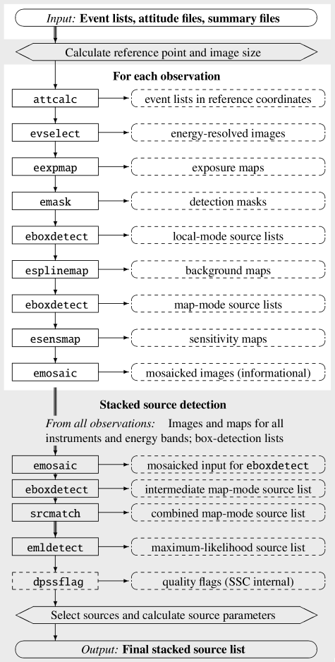
Figure 1: Structure of the task edetect_stack. Internal steps are shown in hexagonal boxes, calls to external SAS tasks in rectangles, and their data products in dashed rounded boxes. Stages dealing with all observations simultaneously are highlighted by a grey background. In ‘local mode’, eboxdetect uses an internally determined local background value, while in ‘map mode’ an external background map is applied. This is produced by esplinemap, which is named after its first functionality and now run in its new adaptive-smoothing mode (Sect. 2.2).

ESA’s X-ray mission, XMM-Newton (Jansen et al. 2001), launched in December 1999, is dedicated to pointed X-ray and ultraviolet to optical observations. Its large field of view and effective area also make it suitable for survey-like searches for serendipitous X-ray detections. Up to one hundred (or more) sources are found in addition to the main target in each XMM-Newton observation with the EPIC CCD instruments pn(Strüder et al. 2001), MOS1, and MOS2 (Turner et al. 2001). The XMM-Newton Survey Science Centre Consortium (SSC, Watson et al. 2001) has been generating catalogues of individual detections, merged into unique sources, from public XMM-Newton observations since the beginning of the mission. The series of XMM-Newton Serendipitous Source Catalogues are produced from pointed observations with the EPIC instruments. The most recent data release 3XMM-DR8 of the third generation catalogue was published on May 16th, 2018. The catalogue series and the underlying software are described by Watson et al. (2009, hereafter: Paper V) and Rosen et al. (2016, hereafter: Paper VII). Complementary source catalogues are the Slew Survey Source Catalogue (Saxton et al. 2008) from EPIC-pn data taken during telescope slews and the XMM-Newton OM Serendipitous Ultraviolet Source Survey Catalogue (Page et al. 2012) from data taken with the Optical Monitor. The software to reduce and analyse XMM-Newton data and to compile the catalogues has been developed by the SSC and the XMM-Newton Science Operations Centre (SOC) and is released regularly by the SOC.

After seventeen years in orbit, XMM-Newton has re-observed many patches of the sky. Overall, almost a third of the XMM-Newton sky has been visited more than once. This may occur from planned repeated observations of variable objects or calibration targets, mosaic observations of large regions, or unplanned overlaps of independent observations. To properly exploit the survey potential of the growing body of multiply imaged sky areas in the XMM-Newton archive, we (members of the SSC) have now developed a new standardised approach to source detection in multiple observations. Previous work on overlapping observations includes the ROSAT catalogues (Voges et al. 1999; Boller et al. 2016), for which the photons of all exposures covering a sky region are merged, the SwiftFT (Puccetti et al. 2011) and 1SXPS (Evans et al. 2014) catalogues, for which overlapping images are merged, and the upcoming second release of the Chandra Source Catalogue (Evans 2015), for which the photons of observations with aim-points within 1′ are merged. For the XMM-Newton EPIC data with a strongly position-dependent point spread function (PSF), we perform simultaneous multi-band PSF fitting in all individual images without merging them. A maximum-likelihood algorithm is employed in the five standard energy bands (1) 0.2$-$0.5 keV, (2) 0.5$-$1.0 keV, (3) 1.0$-$2.0 keV, (4) 2.0$-$4.5 keV, and (5) 4.5$-$12.0 keV. This is similar to the method used to produce the other XMM-Newton source catalogues. Parameters of each source are derived from overlays of the empirical PSFs for the respective instrument, energy band, and off-axis position. The full procedure from the input event lists to the final stacked source list has been made available to all users within the XMM-Newton Science Analysis System (SAS, Gabriel et al. 2004).

This paper, number VIII in the series of publications dedicated to the catalogues of serendipitous detections in XMM-Newton pointing-mode observations, introduces the first catalogue of X-ray sources from spatially overlapping EPIC observations. Being the first release using stacked source detection, it also serves as a method validation and as a feasibility study. It has been compiled from a selection of good-quality data, namely overlapping 3XMM-DR7 observations with large usable chip area and reasonably low background. All sources in the groups of selected observations are included in the catalogue, whether detected in overlapping or non-overlapping parts of their fields of view. Within the series of XMM-Newton serendipitous source catalogues, it is named 3XMM-DR7s.

The following Section 2 describes the data processing and source detection on multiple observations, an implementation of an adaptive smoothing technique to model the background in the images, and the detection efficiency and sensitivity for overlapping observations. Section 3 contains the selection criteria of the observations that enter the first stacked catalogue and a new automated strategy to identify and reject observations with a high background throughout the whole observation. Section 4 covers the compilation of the catalogue and describes its properties and the access it and to the auxiliary products. Section 5 gives information on planned future catalogue versions and a summary.

2 Data processing and source detection

The new catalogue 3XMM-DR7s is based on archival XMM-Newton data that entered 3XMM-DR7. Throughout the paper, we refer to it as the stacked catalogue and to the other releases from source detection on single observations as the 3XMM catalogues. The term ‘stack’ is used for a group of overlapping observations for which simultaneous source detection is performed. In the context of XMM-Newton observations, ‘exposure’ stands for the measurement by one of its instruments within an observation. ‘Images’ are created for each observation, instrument, and energy band separately, if not noted otherwise. If several images are merged into a single file, it is called a ‘mosaic’.

3XMM-DR7s is processed with the SAS software version 16 and calibration files as of July 2017. We follow the data handling outlined in Papers V, VII, and the 3XMM-DR4 online documentation, using the same parameters as in the 3XMM pipeline wherever applicable. The tasks are adjusted to the needs of source detection on multiple observations, including the handling of many input files and large image sizes, runtime improvements, wider ranges of allowed parameter values than in single observations, for example the minimum detection likelihood, and additional output used to create the final stacked source list. The standardised approach to perform stacked source detection on multiple observations has entered the SAS as a new task edetect_stack together with the updates to the existing source-detection tasks. Its structure is illustrated in Fig. 1. It is a combination of newly written Perl code and up to eleven other SAS tasks, comprising three major steps: (i) Input data to source detection are prepared for each observation individually (described in the next two sub-sections). All input images are created with the same binning, reference coordinates, and size, large enough to cover the sky areas of all observations in the stack. (ii) Source detection is run on all input data simultaneously (described in Sect. 2.3) and the results per input image are stored in an intermediate source list. In both steps, edetect_stack determines the appropriate parameter values for the other SAS tasks and calls them. (iii) Sources which enter the final source list are selected and their source parameters calculated from the results of step (ii). For source detection on a single observation, this step is part of the task emldetect. For multiple observations, modifications are needed and a module of edetect_stack refines this functionality of emldetect (described at the end of Sect. 2.3).

2.1 Preparation of the input data for maximum-likelihood source detection

Event lists and attitude files to produce the new catalogue are taken from the set of files used to produce the XMM-Newton Serendipitous Source Catalogues 3XMM-DR5 to DR7. Within the pipeline processing, the event lists are filtered for good time intervals (GTIs) per CCD with a minimum GTI length of 10 s, cleaned of bad pixels and merged per instrument. They are publicly available via the XMM-Newton Science Archive (XSA). For the 3XMM catalogues, time intervals of background flares are identified in the merged event lists for each instrument using an optimised flare filtering method. Observations in mosaic mode have been split into sub-pointings and attributed individual observation identifiers. More details on the pipeline can be found in Paper VII. For the stacked catalogue, the XSA event lists are filtered with the 3XMM GTIs. If two event lists per instrument are available with the same observation identifier, they are combined using the task merge. Within edetect_stack, information about the telescope boresight during the exposure is obtained from the attitude files. Therefore, they are also filtered with the combined GTIs of all EPIC instruments for the stacked catalogue to eliminate erroneously recorded coordinate shifts.

The filtered event lists and attitude files of a stack of observations are passed to the task edetect_stack. It establishes a common coordinate system for the stack from the pointing coordinates in the attitude files, which is used for all subsequent source-detection steps. The events are projected onto reference coordinates in the local tangent plane using the task attcalc. The reference point of the projection is calculated as the average of the minimum and maximum coordinates of all overlapping observations. The size of the sky area covered by them is derived from their pointing coordinates and position angles. Using the projected event lists, the input files for source detection are prepared for each contributing observation individually, namely images and corresponding exposure maps, detection masks, and background maps for the three EPIC instruments and the five 3XMM energy bands over the full sky area of the stack. The images are created in bins of 4″ $\times$ 4″ by the task evselect. Exposure maps are created by eexpmap and give the exposure time per instrument, taking invalid pixels and relative detector efficiency into account. They serve as input to the detection masks and background maps. For the source-detection tasks, a second set of vignetting-corrected exposure maps is produced. Detection masks are created by emask for each instrument and give the valid pixels per image. They are derived from the lowest energy band, which defines the most conservative mask. Background maps are created by esplinemap and give the modelled background in counts per pixel. Its new adaptive-smoothing mode is described in more detail in the next sub-section. In addition to these mandatory input files for source detection, two sets of products are created for purely informational purposes: All input images and those per energy band are combined into mosaics by emosaic to illustrate the stacks. Sensitivity maps are calculated by esensmap per instrument and energy band.

2.2 Modelling the EPIC background by an adaptive smoothing technique

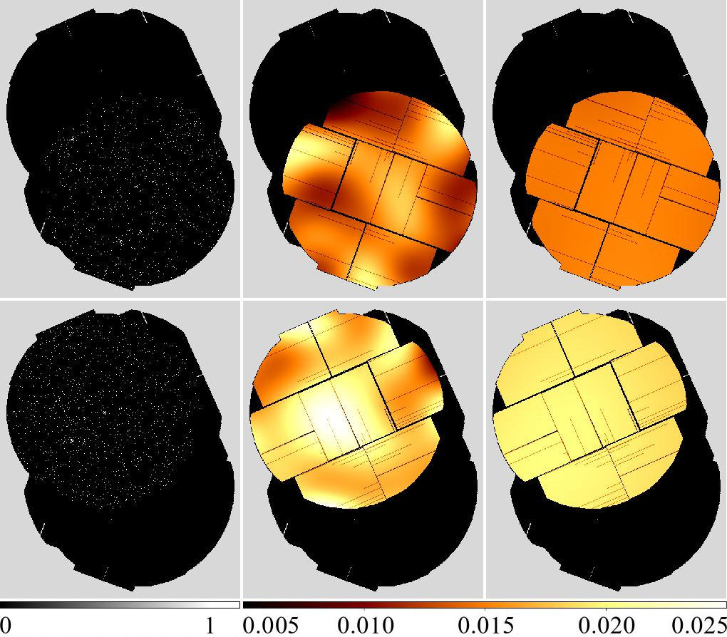
Figure 2: Example of low-amplitude brightness fluctuations in the background maps produced by spline fits: images (left), spline fits (middle), and adaptive smoothing (right) of MOS2 in the 2.0$-$4.5 keV band of a stack of two observations (identifiers 0741033401 and 0741033501). The sky region covered by all instruments is shown in black.

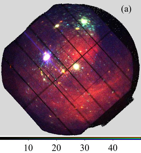
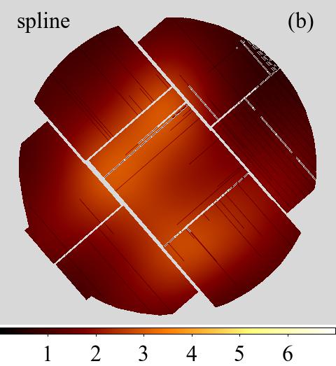
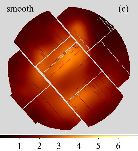
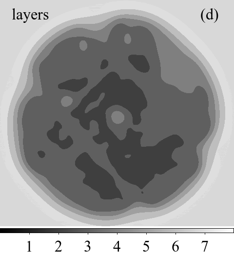
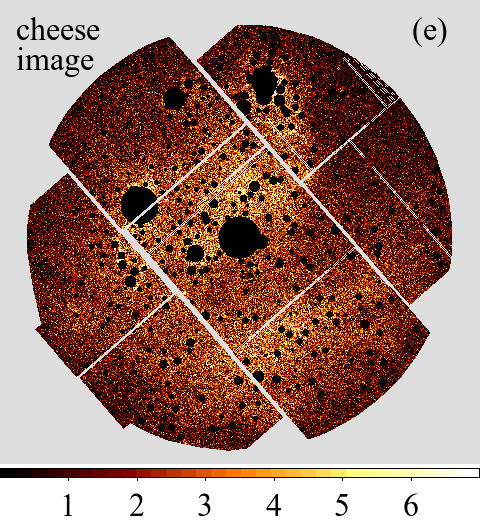
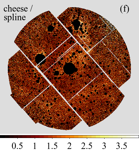
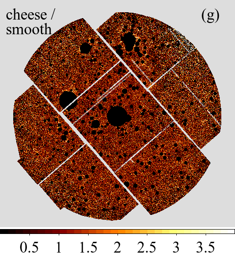
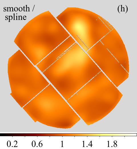
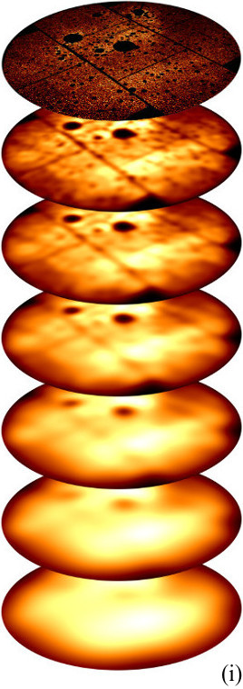
Figure 3: Different methods of background modelling, illustrated in the example of an observation of the $\eta$ Carinae region (obs. id. 0112560101). The panels include a three-band false-colour image of the EPIC observation (0.2$-$1.0 keV, 1.0$-$2.0 keV, 2.0$-$12.0 keV), showing (a) the complex background structure of the field, (b) the MOS1 background map derived from a spline fit and (c) from adaptive smoothing, (e) the source-excised image, (f) and (g) its ratio to the two background maps and (h) the ratio between them. The source-excised image is smoothed with a Gaussian kernel of increasing width (i). All images have a linear intensity scale. The smoothed layers which are chosen per image pixel to construct the background map according to their signal-to-noise ratio are shown in grey-scale (d).

The EPIC background includes an internal instrumental background and external components such as the cosmic X-ray background together with a time-variable local particle background linked to the complex interaction of solar activity with the Earth’s magnetosphere (e.g. Read & Ponman 2003). For source detection, time intervals dominated by high and variable background are filtered from the 3XMM-DR7 event lists(see Sect. 3.2.3 of Paper  VII, ). The remaining background is modelled based on source-excised images by esplinemap and used within the source-detection tasks. To construct the source-excised images, sliding-box source detection is performed on the input images by eboxdetect, run in the so-called local mode, in which a local background level is directly estimated from the image, using a frame around the search box. The resulting list of tentative source positions is passed to the task esplinemap, which excludes circular regions centred at the listed positions within a brightness-dependent radius from each input image.

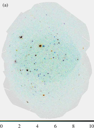
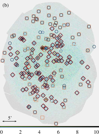
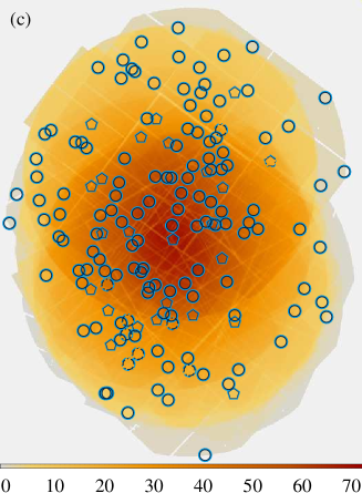
Figure 4: Example of stacked source detection: six overlapping observations within the Magellanic Bridge. (a) Mosaic of all images. The three colour-coded energy bands are: 0.2$-$1.0 keV (red), 1.0$-$2.0 keV (green), 2.0$-$12.0 keV (blue). Colour intensity scales linearly with the number of counts. (b) The same mosaic image with source identifications overlaid. Blue circles and pentagons: 158 sources detected by stacked source detection. Circles mark sources that exceed the likelihood threshold in total or in more than one contributing observation. Red diamonds and boxes: 152 sources detected in the individual observations. Diamonds mark sources that exceed the likelihood threshold in more than one contributing observation. Dashed symbols mark sources that have been flagged by the task dpssflag (cf. Sect. 4.1). (c) Mosaic of the vignetted exposure maps with the identifications of the sources in the stacked catalogue, using the same symbols as in panel (b). The exposure time has been averaged over the instruments and energy bands and is given in units of kiloseconds in the colour bar.

A spline fit has been the standard method to model the background and extrapolate it to the source positions in single observations; this is also employed for the 3XMM catalogues. It gives a reasonably good description of the background behaviour in most images of standard size from single pointings. Test runs, however, have revealed that its current SAS implementation, which was designed for single observations, can result in undesired overshoot or ringing effects for images that are larger than a single XMM-Newton EPIC field of view as needed for stacked source detection (two examples are shown in Fig. 2). The artefacts occur in particular close to the sharp transition between the exposed and the unexposed image area within and outside a single field of view. Furthermore, the splines may smooth out small-scale variations in very complex background structures. Thus, an adaptive filtering method to model the background emission has been introduced in esplinemap as an alternative to the spline fitting. The source-excised images, normalised by the exposure maps, and the corresponding masks are convolved with a Gaussian kernel. The resulting smoothed images are divided by the smoothed masks, compensating for the unknown background flux in the masked source regions. To account for different background structures in individual image areas, an optimum smoothing radius is determined pixel by pixel such that the final adaptively smoothed background map has a uniform signal-to-noise ratio, which limits the allowed noise fluctuations. Therefore, the initial width of the Gaussian kernel is increased by a factor of $\sqrt{2}$ in eight steps. The counts per pixel in the smoothed images are the weighted average over the kernel extent centred at the pixel position. Their Poissonian signal-to-noise ratio is calculated as the square root of the counts under the kernel. For each pixel, the two smoothed images with the signal-to-noise ratios closest to the pre-defined (user-supplied) optimum are selected. The background value with the desired signal-to-noise ratio is linearly interpolated between them. Small-scale structures are thus covered by the images with the narrowest smoothing radii, while the cut-out regions around the sources are filled by values from those with a broad Gaussian kernel. The new default parameters of this method in esplinemap have been chosen empirically as a brightness level of $5\times 10^{-4}$ cts arcsec${}^{-2}\,\textrm{s}^{-1}$ to cut out sources, a minimum smoothing radius of 10 px, corresponding to 40″ when using standard image binning, and a signal-to-noise ratio of 30. For the catalogue images, these values result in a reasonable compromise between minimising the remaining photon noise in the background map and retaining the resolution for true spatial background variations.

The smoothed background maps are generally in good agreement with the input images. For the 26 835 catalogue images, the median deviation between the total counts of the source-excised background maps and images is below 2 %. Figure 3 provides an example comparing the spline-fit background and the results of adaptive smoothing for a single observation of the region of $\eta$ Carinae. The large-scale variation of its complex background structure (Fig. 3a) is well described by the spline fit (Fig. 3b), while small-scale structure becomes additionally visible in the adaptive smoothing fit (Fig. 3c). The differences between the two methods are most obvious in a comparison of the ratios between the source-excised image (Fig. 3e) and the source-excised background maps (Fig. 3f and g) and in a direct comparison of the background maps (Fig. 3h). Figure 3i shows six of the eight layers with increasing smoothing radii, from which the smoothed background map has been constructed, and Fig. 3d the layer chosen for each image pixel. Tests on selected fields with complex background and of large images processed with both methods confirm a more robust approximation of the observed background by adaptive smoothing in these cases. However, it may be less sensitive to extended low surface-brightness sources, in particular if small cut-out radii are chosen for the source-excised images. Adaptive smoothing has been chosen as the standard approach for the new catalogue, whose first version is restricted to fields without large extended emission (see Sect. 3).

2.3 Source detection on stacked images

All data products described in Sect. 2.1 are used in parallel by the source-detection tasks, which couple images, exposure maps, and background maps for each observation, instrument, and energy band, and detection masks for each observation and instrument. Simultaneous source detection is performed by means of the usual two-step process used for XMM-Newton data: sliding-box source detection followed by maximum-likelihood fitting. This was described originally in Paper V. In the following paragraphs, essentials common to source detection on single and on multiple observations are summarised, followed by the modifications introduced for the stacked catalogue. Both detection steps test the null hypothesis that all counts collected arise from random background fluctuations and no source is present. The null-hypothesis probability $P_{\mathrm{null}}$ is converted into a measure for detection significance by the logarithmic likelihood $L=-\ln P_{\mathrm{null}}$, which is given in the XMM-Newton source lists.

First, all images are searched for tentative sources by a sliding-box source detection using the task eboxdetect. The initial run is made with a 20″ box size. Two subsequent runs increase the box size by a factor two each to facilitate searches for extended sources. Detections from previous runs are overwritten if one is found at the same position with a higher signal-to-noise ratio. For each image $i$, a logarithmic likelihood

$$L_{i}(c_{i},c_{b})=-\ln P_{\Gamma}(c_{i},c_{b})$$ (1)

is calculated such that the measured counts $c_{i}=c_{s}+c_{b}$ within the detection box exceed the level of pure Poissonian noise. $c_{s}$ are the source and $c_{b}$ the background counts in the detection region. $P_{\Gamma}$ is the regularised incomplete gamma function

$$P_{\Gamma}(a,x)=\frac{\int_{0}^{x}e^{-t}t^{a-1}dt}{\int_{0}^{\infty}e^{-t}t^{a-1}dt},$$ (2)

used here as the cumulative distribution function of a Poisson distribution. According to Fisher (1932), the natural logarithms of probabilities $P_{i}$ from $n$ independent tests of the same null hypothesis can be combined as $=-2\sum_{i=1}^{n}{\ln{P_{i}}}$, which follows a $\chi^{2}$ distribution with $2n$ degrees of freedom. The detection likelihoods of a source in $n$ individual images is hence calculated as

$$\textrm{LIKE}_{\textrm{eboxdetect}}=-\ln\left(1-P_{\Gamma}(n,\sum_{i=1}^{n}{L_{i}})\right),$$ (3)

making use of $P_{\Gamma}$ as the $\chi^{2}$ cumulative distribution function. The combined EPIC detection likelihoods are also called ‘equivalent likelihoods’, referring to Fisher (1932). All images are considered for which the source position lies within the detection mask. Their number can thus vary from source to source within one detection run. Sources are selected if their equivalent likelihood exceeds a pre-defined minimum, and passed to the task emldetect to calculate their parameters by maximum-likelihood fitting. A good likelihood cut represents a compromise between being as complete as possible with respect to real sources and as strict as possible with respect to spurious detections.

The equivalent likelihood depends on the number of photons in the detection box and on the number of images over which they are distributed, because the large number of images in multiple observations leads to large corrections when combining their individual detection likelihoods according to Eq. 3. In particular, the sensitivity of the sliding-box detection decreases if few counts are distributed over an increasing number of images (cf. Sect. 2.4). To avoid the loss of real sources solely because of the number of images of multiple observations, the stacked box detection step was hence reduced to the same number as used for a single observation: one image for each EPIC instrument and energy band, limiting the number of images $n$ in Eq. 3 to fifteen. Therefore, the corresponding images of all contributing observations are summed per instrument and energy band by the task emosaic within edetect_stack; likewise the corresponding exposure maps, background maps, and detection masks. These mosaics are exclusively used in the sliding-box run. However, transient sources that are significant in a subset of the observations may disappear from the pre-selection if box detection is restricted to the mosaics. Thus, eboxdetect is also called for each observation separately. For the stacked catalogue, a likelihood cut of five is used in all eboxdetect runs. The source lists of all observations and the one based on the mosaics are merged by srcmatch within a fixed radius of $2\sqrt{2}$ times the pixel size, chosen to cover the area of two by two pixels. The matching radius for standard images with a default binning of 4″ thus becomes 11.3″. The likelihood column of the merged source list holds the maximum detection likelihood of a source.

Next, the task emldetect determines the parameters of all sources in the merged box-detection source list in all images per observation, instrument, and energy band simultaneously by means of maximum-likelihood fitting. Details on the approach and the parameters chosen for the catalogue processing are given in Sect. 4.4.3 of Paper V. All input images are combined with their respective background image, exposure map, and detection mask. In each image, the appropriate PSF is chosen at the tentative source position for the instrument configuration. The common source position and extent and the counts per image are fitted within an area of 1′$\times$1′ in all images for which the PSF overlaps with the field of view as defined in the detection mask. emldetect scales each PSF with the counts measured in the image. Thus, it does not need to merge PSFs a priori and to make assumptions about the source spectrum. The detection sensitivity is then approximately the same for all incident source spectra (Stewart 2009) and nearly independent of the accuracy of the instrument cross-calibration. To choose the sources that are considered real and to minimise the spurious content, a significance level needs to be defined. For each source, the detection likelihood in the given fitting setup is derived using the best-fit C-statistic (Cash 1976, 1979), minimising the sum of the deviations

$$C_{i}(c_{i})=2\sum_{k=1}^{N}(m_{k}-c_{k}\ln(m_{k}))$$ (4)

between measured counts $c$ and the model prediction $m$ in a region of $N$ pixels, where $c_{i}$ stands for the sum of source counts $c_{s}$ and background counts $c_{b}$ in the detection region as before. It is compared to the null hypothesis that the signal purely arises from background counts $c_{b}$, resulting in the logarithmic likelihood ratios $\Delta C_{i}=C_{i}(c_{i})-C_{i}(c_{b})$. According to Cash (1979), the $\Delta C$ values follow a $\chi^{2}$ distribution with $\nu$ degrees of freedom, which is the number of varied parameters. The $\Delta C_{i}$ of the $n$ images involved are combined into the equivalent likelihood

$$\textrm{DET\_ML}_{\textrm{emldetect}}=-\ln\left(1-P_{\Gamma}(\frac{\nu}{2},\sum_{i=1}^{n}\frac{\Delta C_{i}}{2})\right),$$ (5)

using the regularised incomplete gamma function $P_{\Gamma}$ (Eq. 2). The likelihood values are then a measure for detection significance that the collected counts exceed random background fluctuations. The $\nu$ free parameters are the coordinates of the source, its extent, and the counts per image in which the source lies within the instrumental detection mask. If the likelihood of the source being extended falls below a threshold of four or its extent radius below 6″ (see Paper  V, ), the source extent is set to zero and $\nu$ is reduced by one to $n+2$. Using these definitions, the degradation of the detection sensitivity with the number of images for faint sources is less prominent than for eboxdetect (cf. Sect. 2.4), and emldetect is applied to all images of the stack simultaneously. Deviating from the standard procedure for individual observations, emldetect is called by edetect_stack with a minimum detection likelihood of zero to store the parameters of each box-detection source and each image in an intermediate source list without (de-)selecting sources.

A separate module of the task edetect_stack is dedicated to the calculation of the final source parameters, to performing a quality assessment, and to source filtering. In particular, the total equivalent likelihood over all observations and the likelihoods for each individual observation are calculated for each detection. Sources are included in the final source list if at least one of these equivalent likelihoods exceeds a user-defined minimum. As in the 3XMM catalogues, a likelihood of at least six is required in the stacked catalogue. An example of stacked source detection on archival observations of the Magellanic Bridge region is shown in Fig. 4. For comparison, emldetect was also run for each observation separately. The resulting detections are joined within a matching radius of 15″, the radius used to create the 3XMM catalogues of unique sources, and shown in red in Fig. 4b. A comparison between source lists from stacks and individual observations is given in Sect. 4.4.

The results of edetect_stack are provided in two FITS-format source lists with different structure: one emldetect-like list and one in catalogue-like format. The first is described in the task documentation of emldetect. The second list includes an all-observation all-EPIC summary row for each detected source plus one additional row for each individual contributing observation of this particular source. These latter catalogue-like source lists are the basis of the new stacked catalogue. Details on their columns are found in Sect. 4.1 and Table LABEL:tab:columns.

2.4 Testing detection efficiency and sensitivity with artificial stacks

The efficiency of the new stacked source detection was investigated in several tests using long archival observations. Stacks were constructed by dividing their event lists into shorter ones. Source detection was performed following the recipes given above and a reference source list created from the full exposure.

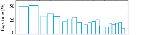
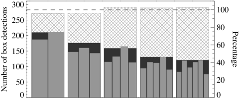
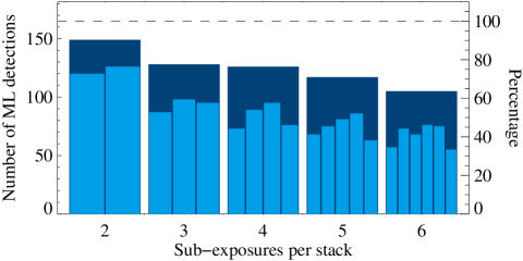
Figure 5: Stacked source detection on an observation split into several nearly equally long sub-exposures (obs. id. 0555780201). Upper panel: Percentage of exposure time. Middle panel: Sliding box detections that are submitted to emldetect. Cross-hatched bars mark those found in the fifteen mosaics of all sub-exposures, dark filled bars the detections found when running eboxdetect on all individual images simultaneously, and light filled bars the box detections in each individual sub-exposure. Lower panel: Final maximum-likelihood detections with a minimum total detection likelihood of at least six in the stack (dark blue) and in the individual sub-exposures (light blue). The dashed horizontal line marks the result of source detection on the full, unsplit observation.

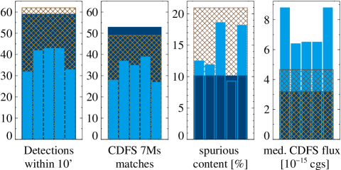
Figure 6: The five-component artificial stack from Fig. 5 compared to the CDFS 7 Ms catalogue within a 10′ circle. From left to right: All XMM-Newton detections, those with a Chandra match within 5″, fraction of detections without Chandra counterpart, and Chandra full-band fluxes of the matches. Dark blue bars denote the results from stacked source detection, light blue bars those from source detection on the individual sub-exposures, and orange cross-hatched bars their joined source lists.

In the first experiment, the detection efficiency and its dependence on the number of overlapping observations was investigated. Selected observations with an exposure time of at least 100 ks were split into two to six sub-exposures of similar duration. The results of source detection on the various stacks were compared to those for the full observation. Figure 5 shows an observation of the Chandra Deep Field South, a deep extragalactic survey field (obs. id. 0555780201). As expected, the number of sliding-box detected sources decreases drastically if all input images are used in parallel but remains approximately constant for the corresponding mosaics. A slight increase in box detections with the number of sub-exposures indicates more false positives. The number of maximum-likelihood detected sources also tends to decrease close to the detection limit when the number of sub-exposures increases. The source counts are distributed among more images, resulting in lower detection likelihoods per image, and the fit has more degrees of freedom, resulting in larger corrections when calculating the total equivalent likelihood. The overall sensitivity, hence the number of reliably detected sources is reduced with an increasing number of short sub-exposures. A given source will thus have different likelihood values in a stack or one long observation of the same length despite the correction scheme applied (see below for a quantitative assessment).

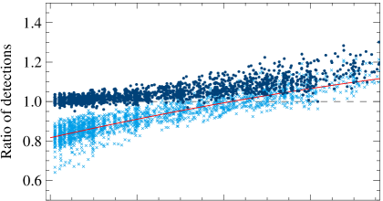
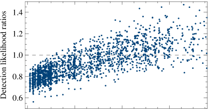
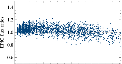
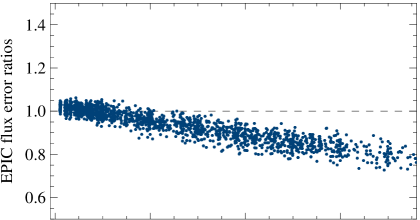
Figure 7: Source parameters derived from stacked source detection in a longer and a shorter part of long observations, compared to source detection in the longer part only. Each dot represents the ratio of the median values of the sources detected in one stack to the median values of the sources detected in the long sub-exposure alone. Sources with an equivalent detection likelihood above six in at least one exposure are included in the stacked source list. The light blue crosses in the uppermost panel mark the ratio of sources with a total likelihood above six. The red curve is a 2nd-order polynomial fit to guide the eye.

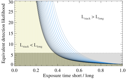
Figure 8: Numerically calculated limiting detection likelihood in stacks of a long and a short observation. For given counts (source plus background) and exposure time ratios, the detection likelihood $L_{\mathrm{long}}$ in the long observation and $L_{\mathrm{stack}}$ in the stack are calculated. The curves show equal likelihoods $L_{\mathrm{stack}}=L_{\mathrm{long}}$, each for a fixed count number. Counts increase from right to left from 15 to 5 000 in 18 steps of 0.14 dex.

To further investigate the reliability and spurious content of the stacked detections, the artificial five-component stack of Fig. 5 was compared with the 7 Ms catalogue of the Chandra Deep Field South survey (Luo et al. 2017), which is expected to include all detectable sources of the much shorter single XMM-Newton observation. The comparison was restricted to the innermost 10′ of the Chandra field, corresponding to a Chandra flux limit of about $4\times 10^{-16}\,\textrm{erg\,cm}^{-2}\,\textrm{s}^{-1}$. From the sub-exposures of the artificial EPIC stacks, a joint source list was created by merging the individual lists. Its flux limit is about $2\times 10^{-15}\,\textrm{erg\,cm}^{-2}\,\textrm{s}^{-1}$. Detections were merged within a radius of 15″ (the radius used to create the 3XMM catalogues of unique sources). The EPIC and the Chandra detections were then matched within a radius of 5″, taking the higher source density of the Chandra catalogue into account. Each match is considered a true source and each EPIC detection without a Chandra counterpart is considered spurious, including the considerable fraction of long-term variable sources that were undetectable during the Chandra observation (see Motch et al. 2009). Figure 6 shows the number of sources and the median Chandra full-band fluxes for stacked source detection, for source detection in the individual sub-exposures, and for their combined source list. The flux sensitivity and the number of reliable detections are higher in the stack than in the sub-exposures alone, and the spurious content decreases significantly, in this example by about 50%.

In a second experiment, the detection efficiency for combinations of two observations with different exposure times was investigated. As described in Sect. 2.3, the combined detection likelihood of a source depends not only on the number of photons collected, but also on the number of images used in the fit. The number of images and thus the number of free parameters in Eqs. 3 and 5 increases by the number of energy bands times the number of active instruments in each observation that is added to the stack. For faint sources close to the detection limit, the combined likelihoods decrease if an observation with low likelihood is added to an observation with high likelihood. To quantify the effect, 54 long observations with common properties (full-frame mode, $\geq$99 % chip area usable for serendipitous science, clean exposure time above 75 ks in all instruments) were selected. They were divided into two parts to construct artificial stacks. The longer exposure has a fixed length, while the shorter one is increased in uniform time steps. Four setups are chosen. The first combines a long sub-exposure that covers 50 % of the total effective exposure time and a short sub-exposure that covers 5 %, 10 %, 15 %, …of it. The second combines a 65 % part and multiples of 2.5 % exposure time, the third an 80 % part and multiples of 2 %, and the fourth a 90 % part and multiples of 1 % exposure time. For the resulting more than 1 800 pairs of a long and a short exposure, stacked source detection is run to compare the results to single detection on the longer alone.

Figure 7 shows how the detection likelihoods and source parameters depend on the exposure time ratios between short and long part (see Table LABEL:tab:columns for the definitions of the stacked source parameters). In general, the detection likelihood and thus the number of sources increase with exposure time, while the statistical errors on the source parameters decrease. For two sub-exposures with an exposure time ratio of at least about 40 %, more and fainter sources are reliably detected in the stacks than in the individual sub-exposures. For lower exposure time ratios, the median detection likelihood and the number of sources above the detection limit decrease for purely statistical reasons, because more degrees of freedom of the fit enter Eq. 5. The limiting exposure time ratio above which the total detection likelihood increases with respect to the single detection depends on the signal-to-noise ratio and on the detection likelihood itself. The dependence can be estimated by a simplified simulation using the eboxdetect definition of detection likelihoods given in Eqs. 1 and 3. For a fixed number of counts in the long observation with 15 images, the equivalent detection likelihood is calculated and compared to the combined likelihood of this long and a short observation. Counts are assumed to scale linearly with exposure time and to be the same in each of the fifteen images of an observation, while in real observations, counts depend on energy band and instrument characteristics. The source counts among the chosen total counts are derived for which the detection likelihood in the long observation $L_{\mathrm{long}}$ equals the likelihood in the stack $L_{\mathrm{stack}}$. Equal detection likelihoods $L_{\mathrm{stack}}=L_{\mathrm{long}}$ are shown in Fig. 8 for different numbers of counts as a function of the exposure time ratio. Sources whose likelihood in the long observation lies above the curve are recovered in the stack with a higher detection likelihood. Sources below the curve have a lower likelihood in the stack and may be lost if they fall below the detection limit of six (dotted horizontal line). The effect is less prominent for the emldetect likelihoods which are based on $C$ statistic but still depend on the number of degrees of freedom of the fit. The simulation confirms the empirical finding that higher detection sensitivity is reached for exposure-time ratios above 0.35$-$0.60, depending on the count number.

The stacked catalogue thus includes all sources which reach the minimum detection likelihood in at least one observation (dark blue dots in the uppermost panel of Fig. 7) or in total. This approach preserves strongly variable sources. It is possible, however, that some of the additional sources with total detection likelihood below the threshold of six are spurious. A simple filtering expression may be applied to the source list to extract sources with total detection likelihood above six only.

3 Field selection for the catalogue

The catalogue of sources in overlapping observations is based on the data used to compile 3XMM-DR7 and its selection criteria: Per observation, each EPIC exposure enters 3XMM if it has a minimum net exposure time of 1 ks, which is the sum of good-time intervals after filtering the event list, and non-empty images in all five energy bands. This first release of a stacked catalogue comprises good-quality observations on which additional requirements regarding observational setup and usability are imposed. These are introduced in the following sub-sections.

3.1 Determining continuously high background

Observations with very high particle-induced background need to be identified before performing source detection for the stacked catalogue since their low signal-to-noise can lower the overall detection likelihoods of sources in the field and cause loss of sources. For the 3rd generation of the Serendipitous Source Catalogues 3XMM, an optimised flare filtering technique was introduced, described in Sect. 3.2.3 of Paper VII. The count-rate threshold of the background light curve above which time intervals are rejected is automatically determined from its signal-to-noise ratio. This method efficiently excludes intervals of high flaring background which are shorter than the total exposure, but is less capable of identifying images with persistently high background or features not resolved by source detection and thus regarded as part of the background, examples of which are given in Fig. 9. We employ a new standardised approach to determine the mean background level of an observation from broad-band background images and use it to find remaining high background emission after applying the good-time intervals from the 3XMM flare filtering. The method is described in Appendix A and applied to all 3XMM-DR7 exposures taken in full frame, extended full frame, or large window mode to establish a high-background cut. For each instrument, probabilities are derived from their median background rate per unit area that measure the background level of the full observation. From trial runs of source detection on combinations of high- and low-background fields, we choose a probability threshold of 87 % to exclude observations from the pre-selection for the stacked catalogue, reducing the risk of loss of detections because of background contamination. Using this cut, the majority of the observations flagged by the DR7 screeners are also discarded by the automatic procedure and 537 additional observations (overlapping or not) are newly defined as affected by high-background, like the examples shown in Fig. 9.

3.2 Selection criteria and grouping of observations

Observations are selected for the first stacked catalogue if they fulfil the following criteria (the number of the 9 710 DR7 observations remaining after each filtering step given in brackets):

1. All three EPIC instruments were active (8 022) and

2. each EPIC instrument was operated in full-frame mode, including Extended Full-Frame Mode for EPIC-pn (6 937).

3. At least 99 % of the chip area are usable according to a classification of OBS_CLASS$\leq 2$ in 3XMM-DR7 (4 741).

4. The mean background level of each instrument (pn: quadrant) lies below the threshold defined in Sect. 3.1 (4 370).

5. The observation overlaps with another one by at least 20 % in area, approximated as an angular separation of up to 20′ between the aim points (2 207).

OBS_CLASSes indicate the fraction of the usable chip area and are adopted from 3XMM-DR7 without further revision. The assignment of an OBS_CLASS depends on a combination of automatic flagging, manual flagging, and background properties within a partly subjective screening process. By using a maximum OBS_CLASS of two, we are aiming at excluding complex background structures and large extended objects, which are not the main interest of serendipitous source detection. The fractional area may be slightly different for similar observations of the same field, possibly resulting in different OBS_CLASSes.

The resulting list of stacks includes three well-studied survey fields that cannot simply be supplied to edetect_stack as a black box, namely M31 and the extra-galactic surveys XXL North and South. Numerous source candidates in the bright core of M31 and the large extent of the XXL surveys prevent them from being processed within a reasonable runtime on standard PCs, which were employed to compile the catalogue. Observations of the M31 core are thus manually de-selected, and 28 observations of its outer parts remain in the catalogue. The large associations comprising the XXL surveys are composed of more than a hundred members each and are completely discarded.

All adjacent overlapping observations are sorted into one group or ‘stack’. The final sample includes 1 789 observations in 434 stacks, the majority of them having two or three members. The number of observations per stack size is given in Table 1.

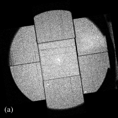
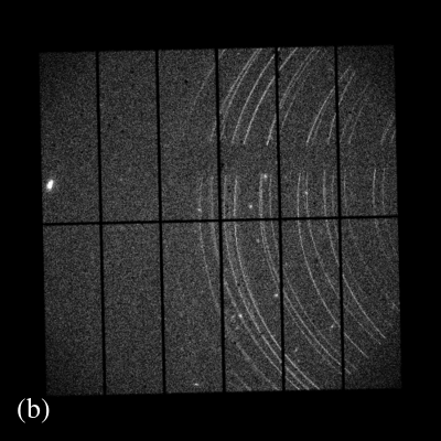
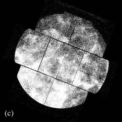
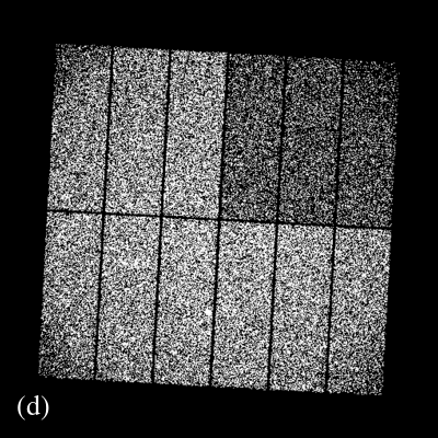
Figure 9: Examples of different types of increased background intensity in EPIC observations which have been assigned a Cauchy probability above the limit of $87\,\%$ and do not have a HIGH_BACKGROUND warning flag in 3XMM-DR7: (a) continuously high background, exceeded by few sources only (obs. id. 0200171401 MOS1), (b) single reflection patterns, caused by a bright X-ray source outside the field of view, but close to it (obs. id. 0604820101 pn), (c) extended diffuse emission (obs. id. 0650220201 MOS2), (d) different brightness levels of the EPIC-pn quadrants owing to continuous counting mode (obs. id. 0406752601). The images are created with a linear brightness scale ranging from zero to half their exposure time in kiloseconds.

4 Catalogue construction and properties

4.1 Organisation of the catalogue

For each of the observation groups described in Sect. 3, stacked source detection is run using the new task edetect_stack. The stacked catalogue is constructed from the unique source lists of the 434 stacks and comprises 71 951 sources. It lists the parameters from the combined fit for each source and, in addition, one row for each observation that was involved in this fit. All source parameters are directly derived from the results of the simultaneous fit to all observations in a stack. Values per observation refer to the subset of images taken during this observation. The catalogue can be reduced to the one-source-one-row layout of the 3XMM slim source catalogues using a selection expression on the identifier columns given below, such as N_CONTRIB. Its columns are mostly organised in the style of the 3XMM catalogues with the same definitions of their values wherever applicable and fully listed in Table LABEL:tab:columns of the Appendix. In this section, we describe the most relevant parameters, modifications to the 3XMM column definitions, and newly introduced columns.

Source identifier. The unique source identifier SRCID in the stacked catalogue is a 16-digit number, composed of a preceding ‘3’, linking it to the convention of the 3XMM catalogues that the detection identifier of individual detections starts with a ‘1’ and the source identifier of unique matches between them starts with a ‘2’, followed by the lowest OBS_ID of the contributing observations (10 digits), and the identifier within the emldetect source list (5 digits), for example 3020624020100030 for the thirtieth detection in a stack with 0206240201 being the lowest identifier of all the observations for which the detection was in the field of view. The five-digits identifiers are not continuous, because the temporary emldetect source list comprises all input detections, and only the significant ones among them are transferred to the final source list.

Each source is attributed an IAU name of the form 3XMMs Jhhmmss.s$\pm$ddmmss, including the truncated sexagesimal right ascension and declination of the source. It is given in the column IAUNAME.

Observations included. N_OBS gives the total number of observations per stack and N_CONTRIB the number of contributing observations for which the source position is inside the field of view. Both column values are set to null (undefined) in the observation-specific rows and can thus be used to select the summary rows per source.

Table 1: Stacks from which the new catalogue is compiled. (a) Number of observations per stack. (b) Number of stacks.

(a)	(b)	(a)	(b)	(a)	(b)
2	269	11	2	22	1
3	74	12	3	23	1
4	16	13	1	24	2
5	14	15	2	25	2
6	15	16	1	28	1
7	4	18	2	32	1
8	5	19	4	49	1
9	4	20	1	52	1
10	4	21	2	66	1

Source coordinates. The position of the source is considered to be the same in all contributing observations and images in the simultaneous fit, while the source counts are determined separately per image (see Sect. 4.5 for a discussion of the astrometric accuracy). It is given in equatorial, galactic and image coordinate systems in the RA, DEC, LII, BII, and X_IMA, Y_IMA columns. Image coordinates refer to the common coordinate system of each stack (Sect. 2.3) and are listed together with their individual errors $\sigma_{\textrm{X\_IMA}}$, $\sigma_{\textrm{Y\_IMA}}$. The combined position error RADEC_ERR is calculated from them as $(\sigma_{\textrm{X\_IMA}}^{2}+\sigma_{\textrm{Y\_IMA}}^{2})^{0.5}$, converted to arcseconds. For symmetric errors in both dimensions, RADEC_ERR/$\sqrt{2}$ is the one-dimensional $1\sigma$ position error, giving the interval that includes 68 % of normally distributed coordinate values. $\sqrt{2.3/2}\times$RADEC_ERR is the two-dimensional error, giving the radius of a circularised ellipse that includes 68 % of normally distributed pairs of coordinates.

Equivalent detection likelihoods. Maximum detection likelihoods are determined per input image, summed, and converted from the total number of degrees of freedom to the mathematical equivalent of a two-parameter fit (see Sect. 2.3). The number of degrees of freedom is two for point sources and three for extended sources plus the number of images involved in the fit (equalling the number of instruments in each observation, for which the mask is valid at the source position, times the number of energy bands) and varies from source to source. The decision whether a detection enters the final source list is based on the equivalent likelihoods. Sections 2 and 4.4 describe how a large number of input images can affect them and thus the source selection in the fitting process. Sources with a minimum equivalent likelihood of six in the whole stack or at least one contributing observation are included in the stacked catalogue.

Source flux. The fitted count rate per image is converted to flux using the energy conversion factors (ECFs) of Paper VII. All-EPIC fluxes are means of the fluxes per instrument and observation weighted by their inverse squared errors. They are null with undefined flux errors but non-zero count errors for an observation if no counts are found within the PSF area of a source. The ECFs depend on the instrument, the observing mode, and the filter used, and on the spectral shape of the source. Therefore, the combined fluxes merging different instruments and setups across the observations are affected by cross-calibration uncertainties (see Mateos et al. 2009). The underlying spectral model of the 3XMM ECFs is an absorbed power law with a column density of $3\times 10^{20}\,\textrm{cm}^{-2}$ and a photon index of 1.7.

Source extent. The radial extent and extent likelihood of a source are fitted simultaneously in all observations. The $\beta$ model used to parameterise the extent is described in Sect. 4.4.4 of Paper V. Sources with an extent radius below 6″ or an extent likelihood below four cannot be resolved and are considered point-like. Their extent is set to zero and their extent likelihood to null.

Mask fraction. The PSF-weighted detector coverage of a source is given for each instrument separately. It is the fraction of the point spread function, for extended sources convolved with the $\beta$ extent model, falling on valid detector pixels. For one observation, it is conservatively defined as the minimum mask fraction of the five energy bands, indicating the most restrictive mask. The stacked mask fraction is the largest value of the contributing observations, indicating the best one.

Source flags. A modified version of dpssflag, the task also in use for the 3XMM catalogues, is employed for an automated quality flagging to warn the user about complexities in the environment of the source that might affect the significance of the detection or the source parameters and their accuracy. The sources are not visually screened. Strings of nine booleans indicate different potential issues of a detection in total and for each instrument, described in Sect. 7.3 of Paper V. A true EPIC flag means a warning for at least one instrument. The nine booleans are converted to a single integer summary flag STACK_FLAG. Sources with a flag value of ‘0’ come without any warning. Flag ‘1’ indicates reduced detection quality in at least one instrument and observation: low detector coverage or a source position close to another source or to bad detector pixels. The list of known bad pixels is hard-coded within dpssflag. ‘2’ is attributed to potentially spurious sources, for example those found within the PSF radius of another source. Flag ‘3’ in the summary row indicates that the source has received flag 2 in all contributing observations. The integer flags are not directly comparable to the 3XMM SUM_FLAGs, which have been set for individual observations and include additional information from visual screening.

Table 2: Overview of the catalogue of unique sources in spatially overlapping XMM-Newton observations, selected from the 3XMM-DR7 observations taken between 2000 February 3 and 2016 December 15.

Description	Number
Number of stacks	434
Number of observations	1 789
Time span first to last observation	Feb 20, 2000
$-$	Apr 02, 2016
Approximate sky coverage	150 sq. deg.
Approximate multiply observed sky area	100 sq. deg.
Total number of sources	71 951
Sources with several contributing observations	57 665
Sources with one contributing observation	14 286
Sources with flag ‘0’ or ‘1’	69 526
Total detection likelihood of at least six	64 221
Total detection likelihood of at least ten	53 492
Extended sources (radius $\geq 6\arcsec$)	3 346
Point sources with VAR_PROB$\leq$1 %	5 607
Point sources with VAR_PROB$\leq$10-5	1 927

Long-term variability between observations. Three new sets of parameters inform about the inter-observation variability of a source, based on typical EPIC count numbers in the Gaussian regime: (i) the $\chi^{2}$ of the long-term flux changes and the associated probability that they are consistent with the flux measurements of a non-variable object, (ii) the ratio between maximum and minimum flux with its 1$\sigma$-error, and (iii) the maximum flux variation in terms of sigma. They are directly derived from the EPIC fluxes and flux errors in all contributing observations and in each energy band, resulting in six columns per quantity.

$$\textrm{VAR\_CHI2}=\frac{1}{n-1}\sum_{k=1}^{n}\left(\frac{F_{k}-F_{\textrm{EPIC}}}{\sigma_{k}}\right)^{2}$$ (6)

is a reduced $\chi^{2}$ of flux variability between the mean all-EPIC flux $F_{\textrm{EPIC}}$ over all observations and the individual fluxes $F_{k}$ derived for each observation, $k$ running from 1 to number $n$ of observations. The associated VAR_PROB describes the probability that the observed flux values are consistent with constant source flux over all observations. It is the cumulative chi-square probability

$$\textrm{VAR\_PROB}=\int_{\chi^{2}}^{\infty}\frac{x^{\nu/2-1}e^{-x/2}}{2^{\nu/2}\Gamma(\nu/2)}dx$$ (7)

to reach at least VAR_CHI2=$\chi^{2}$ at $\nu=n-1$ degrees of freedom. $\Gamma$ denotes the gamma function. A low VAR_PROB thus indicates a high chance that the source shows inter-observation variability.

$$\textrm{FRATIO}=F_{\textrm{max}}/F_{\textrm{min}}$$ (8)

gives the ratio between the highest and the lowest flux recorded across the observations, and

$$\textrm{FRATIO\_ERR}=\left(\frac{\sigma_{F\textrm{min}}^{2}}{F_{\textrm{min}}^{2}}+\frac{\sigma_{F\textrm{max}}^{2}}{F_{\textrm{max}}^{2}}\right)^{0.5}\,\frac{F_{\textrm{max}}}{F_{\textrm{min}}}$$ (9)

its 1$\sigma$ error.

$$\textrm{FLUXVAR}=\max_{k,l\in[1,n]}\frac{|F_{k}-F_{l}|}{\sqrt{\sigma_{k}^{2}+\sigma_{l}^{2}}}$$ (10)

is the largest difference between pairs of fluxes in terms of sigma, with $k$ and $l$ running from 1 to number $n$ of observations.

Observation characteristics. Each row per observation includes the modified Julian dates of its start and end time, the filter, the instrument mode, and the mean position angle of the spacecraft. In the summary row, the beginning of the first and the end of the last contributing observation are given.

Columns copied from 3XMM-DR7. For sources with a counterpart in the 3XMM-DR7 catalogue of sources, information on position, quality flag, and intra-observation variability of the 3XMM-DR7 source are copied to the summary rows of the stacked catalogue. The observation-specific rows list the parameters of the 3XMM-DR7 detection that contributes to the unique source, if one is found. Column DIST_3XMMDR7 gives the distance between the stacked detection and the 3XMM-DR7 counterpart. More details on the matching can be found in Sect. 4.7.

4.2 General characteristics

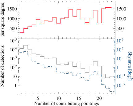
Figure 10: Number of detections (grey solid), detections per square degree (red solid), and approximate sky coverage in square degrees (blue dash-dotted) per number of contributing observations.

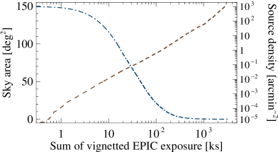
Figure 11: Sky area (blue dash-dotted) and source density (brown dashed) as an approximate measure of detection sensitivity over the total EPIC exposure times of the catalogue stacks. The plot shows the vignetted exposure time averaged over the five energy bands and summed for the three EPIC instruments pn, MOS1, and MOS2.

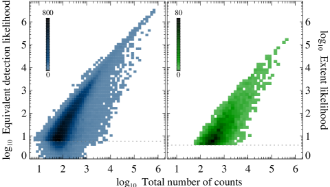
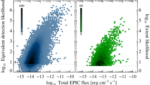
Figure 12: Relation of stacked detection and extent likelihoods to source flux and counts in 3XMM-DR7s. Dotted lines mark the lower limits: minimum detection likelihood to include a source in the source list and minimum extent likelihood per fit to consider a source extended. Colour density scales with the source number per plotting bin.

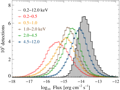
Figure 13: Flux distribution in the catalogue of sources from overlapping observations, in total (grey, filled) and for each of the five energy bands (energy increases from left to right).

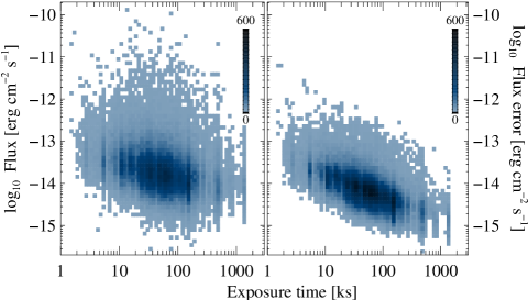
Figure 14: Relation between exposure time EP_ONTIME and all-EPIC fluxes (left panel) and flux errors (right panel) in 3XMM-DR7s. All-EPIC fluxes are the weighted means of the fluxes in the individual energy bands. The exposure time is summed over all contributing observations. Colour density scales with the source number per plotting bin.

The 71 951 unique sources in the stacked catalogue are detected in 1 789 observations in 434 stacks, covering more than sixteen years of observations in total. The longest time span for a single source is 14.5 years. 96.6 % of the sources have been assigned a good automatic quality flag of 0 or 1, and 74.3 % are detected with a total likelihood of at least ten; a somewhat smaller share than in the 3XMM-DR7 catalogue of unique sources (80 %), where the detection likelihood of repeatedly observed sources is given as the highest per-observation likelihood, while the total likelihood in the stacked catalogue is calculated using Eq. 5. 57 665 of the sources are covered by more than one observation with a maximum of 23 visits of a source, and 14 286 were observed once. An overview of the catalogue properties is given in Table 2. Since most of the stacks comprise two observations, the majority of sources has been detected twice (Fig. 10). The absolute number of catalogue sources and covered sky area decrease with increasing stack size because few large stacks are included in the catalogue. The relative source density per unit sky area increases with the stack size thanks to the long total exposure (Fig. 11). The figures include the sources from non-overlapping chip areas with one contributing observation.

With the longer total effective exposure time of the stacks compared to individual observations, more counts are collected per source. Hence, the sources are measured with higher detection likelihoods than in single observations, extended sources additionally with higher extent likelihood, and more sources are detected. The likelihood distributions in the stacked catalogue over total exposure time per source are shown in Fig. 12. In its left panels, the effect of the modified likelihood cut becomes obvious. While a hard cut of six has been applied to the other 3XMM catalogues, 7,730 sources with a total equivalent detection likelihood below six are present in the stacked catalogue: They exceed the threshold in at least one contributing observation, not in the whole stack. A hard cut of four is applied to the extent likelihood, simultaneously determined from all contributing observations.

The distribution of source fluxes in the stacked catalogue – in total and per energy band – is shown in Fig. 13. It is similar to the distributions determined from the other 3XMM catalogues, in agreement with the expectation that the fluxes derived by stacked source detection are consistent with those derived from the individual observations, but better constrained.

Almost 4.7 % of the catalogue sources are resolved as extended with a core radius of the $\beta$-profile extent model of at least 6″. In general, the characterisation of extended sources is affected by larger uncertainties than that of point sources: their intensity profile is less sharp, imposing larger position errors on extended sources, and the beta function is only an approximation to the true extent profile, imposing uncertainties on the measured extent radius, which is a free parameter of the fit. For short observations and faint extended sources, the measured extent relates to the exposure time if insufficient counts are collected to describe them reliably. In stacked source detection, the source extent can now be fitted simultaneously in all observations irrespective of their individual exposure time, making use of the total counts. While uncertainties remain, for example owing to deviations from the true extent profile of a source, the extent parameters can be determined more precisely, and the risk of fitting background fluctuations by spurious extended sources is lower. The experiments with artificial stacks (Sect. 2.4) confirm that extended sources are detected more reliably even if observations of different durations are combined. The high percentage of sources with quality flag 0 or 1 among all extended sources, similar to the one among the point sources, also indicates reasonably low spurious content. Still, large position errors and quality flags 2 and 3 should be taken as signs that an extended detection is uncertain.

4.3 Accuracy of the source parameters

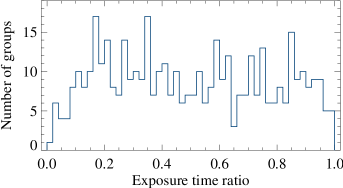
Figure 15: Distribution of exposure time ratios for the 269 stacks comprising two observations.

Owing to the larger exposure time and count number of the stacked observations compared to single observations, stacked source detection becomes more sensitive to faint sources, and the flux errors decrease significantly with exposure time, confirmed by the larger number of catalogue sources having low flux and small flux errors at longer EP_ONTIME (Fig. 14). The dependence of parameter accuracy on the exposure time, shown on the example of the flux errors in the right panel of Fig. 14, applies to all error columns in the catalogue. The smaller errors reflect the smaller scatter of possible parameter values and higher fit accuracy in the stacked source detection. XMM-Newton source detection employs the C statistic in the maximum-likelihood analysis, which is distributed as $\chi^{2}$ plus an additive term proportional to $n^{-0.5}$ (Cash 1976, 1979), negligible for large count numbers $n$. The one-dimensional 1$\sigma$ error on a parameter is derived by stepping the parameter until $C=C_{\textrm{min}}+1$ is reached, corresponding to the 68 % accuracy level of a $\chi^{2}$ statistic. The confidence limits of parameters derived from images with few photons in the source-fitting area and of highly coupled parameters may be actually larger than those for $C_{\textrm{min}}+1$, and an additional error component might thus be considered when interpreting the statistical errors on the stacked parameters, for instance regarding fluxes of sources close to the detection limit or position matches in a cross-correlation with other catalogues. For the position error, an estimate is derived in Sect. 4.5.

As demonstrated in Section 2.4, the number of detections in two-observation stacks increases reliably compared to a single observation for exposure time ratios of more than about 0.4 if not taking the likelihoods during the individual observations into account. The distribution of exposure time ratios of these stacks is shown in Fig. 15. In order to investigate the accuracy of the stacked source parameters quantitatively, the code was applied to simulated images and the results compared to the input parameter values. We start from the modelled source images of catalogue observations, which were created by the task emldetect as by-products of our stacked catalogue pipeline. These are the sum of the background maps and the PSF models of all sources that passed the likelihood cut. To maximise the multiply covered sky area, a subset of 108 stacks of two observations with a maximum offset of 1′ between their respective aim points was selected. They comprise a total of 10 925 catalogue sources. For each of their source images, 25 images were simulated by drawing random values from a Poisson distribution around the input brightness of the source image pixel by pixel. On the resulting $108\times 25=2700$ simulated stacks and 5400 observations, source detection was performed. The new source parameters derived from the simulations were compared to the input values on a per-stack and a per-observation basis. The distributions of the offsets from the input values are shown in Fig. 16 for the free fit parameters coordinates and count rate and for the total equivalent likelihood. They are neatly centred at zero, confirming that the true values are reproduced, and are narrower for stacked source detection than for the individual simulations, confirming that the stacked source parameters have a higher precision and accuracy.

4.4 Performance of stacked compared to non-stacked source detection

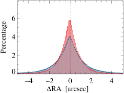
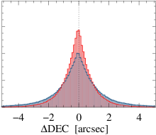
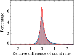
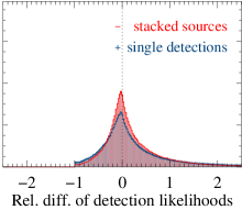
Figure 16: Accuracy of the source parameters of point sources from stacked (red) and non-stacked (blue) source detection, derived from simulated images of stacks comprising two observations. The coordinates in the upper panels are absolute offsets: results of source detection on simulated images minus input value. Count rates and equivalent detection likelihoods in the lower panels are relative differences: simulations minus input divided by the input value.

To quantify the improvement of the detection sensitivity of stacks over individual observations within consistently designed data sets and source-detection runs, source detection has been performed separately on each catalogue observation, using the same method and parameters as applied to the stacks of observations. The 126 658 individual detections were matched into a joint list of 71 921 tentative unique sources within a matching radius of 15″. We compare the stacked sources first with the individual detections and then with the joint sources, again using a radius of 15″. The joint source lists are expected to deviate from 3XMM-DR7 due to the different background models and image creation. Section 4.7 includes a comparison with 3XMM-DR7.

Figure 17 shows distributions of four main source parameters of the stacked catalogue and the individual detections, all normalised to their total number. The longer effective exposure times and smaller flux errors of the stacked catalogue with respect to all detections from the individual observations are clearly visible. The stacked detection likelihoods tend to be higher than that of the individual detections, but include small values for sources that are significant in only one contributing observation. Fluxes are expected to be consistent. Differences in their distributions may indicate a larger share of low-flux sources in the stacked catalogue and better sensitivity to faint sources.

To quantify potential gain and loss of sources in stacks compared to individual observations, the detections that are not recovered by stacked source detection are investigated. 4 931 are found in the single runs only. The vast majority – over 98 % – are detected in one observation with low likelihood without a potential second detection within 15″ although located in overlap areas. About 10 % may be subject to source confusion, overlapping with neighbouring detections within 30″. A large fraction of 40 % of the not recovered ‘single-only’ detections are extended, 416 even with an extent radius of more than 1′. They have large positional uncertainties which may affect the matching, and a high chance to be spurious detections.

For the comparison between the stacked catalogue and the joint source lists, the positions of the merged sources are defined as the mean positions of the contributing single detections and their extent as the maximum extent among them. 4 347 sources are found by stacked source detection only, meaning that they have no counterpart in the joint source list within a 15″ radius. Most of them are located in areas covered by several observations. Only 15.7 % of them are extended, 121 with an extent radius larger than 1′. The point-like stack-only sources tend to have higher detection likelihoods and slightly better constrained fluxes than point-like single-only detections. Together with the experiment described in Sect. 2.4 and Figs. 5 and 6, this clearly indicates that a larger fraction of the stack-only than of the single-only sources are reliable detections and that the spurious source content is significantly reduced by stacked source detection.

Figure 18 illustrates the differences between stacked and non-stacked detections in an example of 19 observations. The images are background-subtracted, normalised by their exposure time per pixel, and combined into a mosaic for display purposes. Plot symbols indicate the significance of the detection, the number of contributing observations, and the source extent. Several joint-only detections are very extended, thus most likely spurious, and disappear in the stack. Additional example images of stacks comprising two to five observations are shown in Fig. 23.

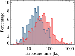
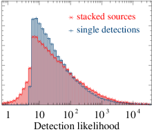
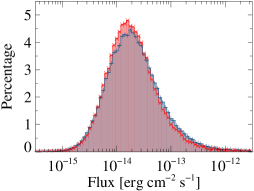
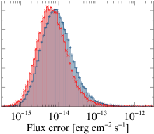
Figure 17: Normalised distribution of all-EPIC good time intervals, detection likelihoods, fluxes, and flux errors of the sources from stacked source detection (red) and of the individual detections in the source lists per single observation (blue).

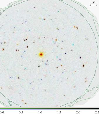
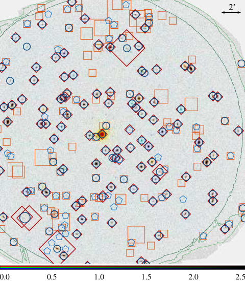
Figure 18: Example with large deviations between stacked and joint source list: nineteen observations of HD 81809. For clarity, the mosaicked image is shown both without and with source identifications. Blue symbols: Sources detected in the stack. Thick circles are used for sources with an equivalent detection likelihood above six in total or in at least two observations, thin pentagons for the others. Red symbols: Joined individual detections. Thick diamonds are used for those merged from more than two observations, thin squares for the others. The plot symbols have a minimum radius of 22″ and scale with the source extent if it is larger than that. The contours enclose areas within at least two (red), seven (orange), and twelve (white) observations overlap.

4.5 Astrometry

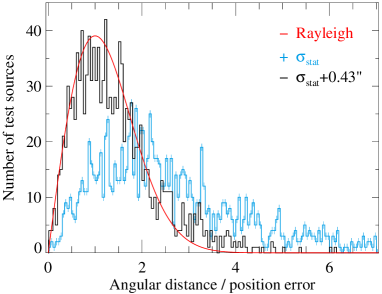
Figure 19: Error-normalised position offsets between sources in the stacked catalogue and associated quasars in SDSS-DR12 compared to a Rayleigh distribution (red). Light blue: Based on the one-dimensional purely statistical position errors RADEC_ERR/$\sqrt{2}$ given in the catalogue. Black: Using the best-fit additional error component 0.43″, linearly added to the statistical error on the X-ray position.

The source positions in the stacked catalogue are determined simultaneously from all observations using their respective calibration. For the 2XMM and 3XMM catalogues, the observations are rectified after performing source detection by comparing the measured X-ray positions of the brightest sources in a field with positions in optical and infra-red catalogues and applying the derived coordinate shifts and field rotation to all sources in the field. The approach cannot be used for the source lists from which the stacked catalogue is compiled, because the different observations per stack might be affected by different shifts. New, more detailed PSF models, upgrades to the source-detection tasks, and a refined boresight calibration have helped to determine the source positions for the 3XMM catalogues more precisely than for previous versions even without this field rectification (see Paper  VII, ). Using them, no additional astrometric corrections are applied to the first stacked catalogue. The stacked position errors from the joint fit are purely statistical uncertainties of the measurements. Systematic uncertainties like the inaccuracies of the (positional) cross-calibration of the contributing observations are thus not included in the stacked catalogue, but can be estimated from the deviations between measured and expected positions of point sources with well-defined astrometry.

For the 2XMM catalogues, the mean additional 1$\sigma$ position error has been determined to be about 1″ before and 0.35″ after astrometric correction from a comparison with optical quasar positions in the Sloan Digital Sky Survey (SDSS), assuming that the error-normalised angular distances are Rayleigh distributed (Paper  V, ). Following this approach, the (uncorrected) X-ray positions of the unique sources of the stacked catalogue are matched with the SDSS release DR12 (Blanton et al. 2017) without further restrictions on off-axis angle or quality flags. As for the other 3XMM catalogues (Paper  VII, ), a matching radius of 15″ is used. The 1 288 quasars among the best matches are selected, and the histogram of their positional offsets $x=\delta/\sigma$ is compared with a Rayleigh distribution $xe^{-0.5x^{2}}$, $\delta$ being the angular distance between the positions in SDSS and in 3XMM-DR7s, and $\sigma$ the combined circularised one-dimensional position errors, namely $(0.5\times(\textrm{errMaj}^{2}+\textrm{errMin}^{2}))^{0.5}$ for SDSS and RADEC_ERR/$\sqrt{2}$ for 3XMM-DR7s. An additional error component on the X-ray position is varied until best agreement between the measured histogram and the Rayleigh distribution is reached. Since the nature of the additional error is unknown, the fit is performed for two alternatives, a quadratic sum $\sigma=({\sigma_{\textrm{stat}}^{2}+\sigma_{\textrm{sys}}^{2}})^{0.5}$ and a linear $\sigma=\sigma_{\textrm{stat}}+\sigma_{\textrm{sys,lin}}$. The best fits are achieved with a quadratically added component of $\sigma_{\textrm{sys}}$=0.73″ and with a linearly added component of $\sigma_{\textrm{sys,lin}}$=0.43″, respectively, which can be considered the parameter range of the mean systematic error on the stacked source positions (not included in the catalogue). Figure 19 shows the position offsets between stacked sources and SDSS quasars normalised by the pure statistical errors, with the linearly added 0.43″ uncertainty on the X-ray positions, and the respective Rayleigh distribution.

For comparison, the same method is applied to the uncorrected positions of the individual detections in 3XMM-DR7. Their distribution of offsets from associated SDSS quasars is fitted with $\sigma_{\textrm{sys}}$=1.01″ and $\sigma_{\textrm{sys,lin}}$=0.59″. In the 3XMM catalogues, errors on the field translation and rotation are determined during the field rectification, and their combination is applied as additional error component. Its median in DR7, restricted to detections with a quasar association, is 0.43″. Although derived from astrometrically uncorrected data, the parameter range of the additional error component for the stacked catalogue is far below the pixel size and smaller than for the individual DR7 detections in the same sample of observations.

4.6 Long-term source variability between observations

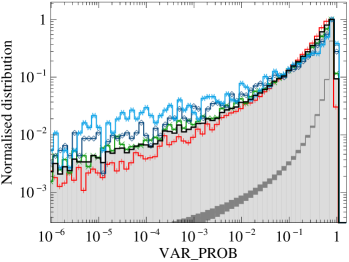
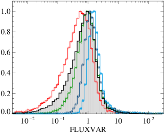
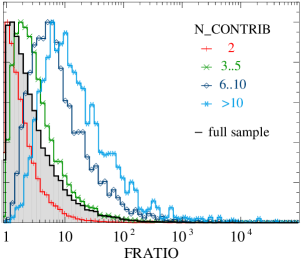
Figure 20: Three of the all-EPIC long-term variability parameters for point sources and their different dependence on the number of contributing observations. A low value of VAR_PROB and high values of FLUXVAR and FRATIO can indicate a long-term variable source. The dark grey area in the left panel indicates the 1$\sigma$ range of the probability estimate for constant sources. All histograms are normalised to their maximum.

The stacked catalogue can serve as a database for long-term variability of serendipitous XMM-Newton sources: Irrespective of the detection probability within a single observation, fluxes and flux errors are determined for each observation that covers the source of interest without the need to match individual detections or to determine upper flux limits, increasing the chance to identify transients. Inter-observation variability in XMM-Newton data has been explored previously by Lin et al. (2012) based on high signal-to-noise detections in 2XMM-DR3i and through the EXTraS project (Exploring the X-ray Transient and variable Sky, De Luca et al. 2016) based on 3XMM-DR5 and slew observations, published as the EXTraS long-term Variability Catalogue (Rosen & Read 2017). Variability in other missions has been discussed for example by Evans et al. (2010, Chandra), Evans et al. (2014, Swift), and Boller et al. (2016, ROSAT).

For each stacked catalogue source that has been observed at least twice with non-zero counts, five quantities describing its inter-observation variability are derived from the total flux and the EPIC fluxes of the contributing observations (see Sect. 4.1). Since they are based on mean fluxes, they provide information on potential long-term variability only and are not probed for intra-observation variability. For 787 detections, an observation-level EPIC flux has been set to null, because no counts were detected during this observation. Null fluxes do not contribute to the variability parameters in the present catalogue. Upper limits for such cases will be included in future releases.

The parameters show little dependence on the energy band, with the highest values being present in the well-populated bands 2$-$4, but clear dependence on the number of contributing observations N_CONTRIB. VAR_PROB is least dependent on it because it is normalised by the degrees of freedom. Distributions of the variability parameters are given in Fig. 20. All histograms peak at higher parameter values for larger N_CONTRIB. This dependence is qualitatively consistent with the results of Rosen & Read (2017). They simulate sparsely sampled long-term light curves for objects with constant mean fluxes, derive the maximum flux variations in terms of sigma, and show their change with the number of light-curve points, owing to larger statistical fluctuations for a larger number of points. More than half of the repeatedly observed sources in the stacked catalogue are covered by only two snapshots. Thus, the distributions for low numbers of contributing observations dominate the overall result. The catalogue does not include boolean variability flags, since the parameter thresholds to consider a source tentatively variable strongly relates to the scientific question to be addressed. For example, 5 607 or 10.2 % of the repeatedly observed point sources in the catalogue have VAR_PROB$\leq$1 %. Using a more restrictive probability cut of $10^{-5}$, 1 927 or 3.5 % point sources can be considered long-term variable. To provide a rough estimate of the false-alarm rate among them, we assume constant flux for all catalogue sources and randomise the observation-level fluxes using Poisson distributed count numbers. This is repeated five hundred times, and the resulting distribution of probability values for non-variable sources included in Fig. 20.

When filtering on high variability, sources with generally unreliable variability parameters should be excluded, in particular detections with poor quality flags and extended sources. Poorly constrained flux values in individual observations and false positives on detector features like bad pixels or stray light may also mimic variability. Many of them can be identified and removed by applying cuts to the errors on the flux ratios. High-proper motion objects and Solar-System bodies cannot be uniquely identified by the source-detection process which assumes stable source positions in all images. For example, the high-proper motion binary 61 Cygni separates into ten individual sources from eighteen overlapping observations in the stacked catalogue, recorded at different levels of (apparent) variability. Visual inspection of the source images which are distributed together with the catalogue (Sects. 4.9 and B.4) helps to reveal these cases.

In the 3XMM catalogues, intra-observation variability is investigated for all detections with at least 100 counts. We select sources with a counterpart in 3XMM-DR7 (see Sect. 4.7) and compare the DR7 parameters on intra-observation variability with the inter-observation variability from this work. Some, but not all of them are expected to be identified on all time scales as variable. A long-term variable source may be constant over the time span of a single observation, and variability on short time scales does not necessarily imply long-term variability of the mean fluxes, as for regular periodicity of up to a few hours. Information on short-term variability is provided for 11 172 point-like DR7 counterparts to stacked sources. 579 are flagged as short-term variable in at least one DR7 observation, and 477 of them have several observations in the stacked catalogue. As expected, a considerable number of short-term variable sources also show signs of long-term variability: 355 with a probability below 1 % that the measurements are consistent with constant flux, 282 with a probability below $10^{-5}$. Thus, 122 of the sources whose DR7 counterpart is flagged as short-term variable are not clearly long-term variable in the stacked catalogue. For 29 of them, the DR7 observation that triggered the short-term variability flag is not part of the sample selected for the stacked catalogue according to the criteria listed in Sect. 3.

To demonstrate the potential of the new variability parameters for transient detection and the advantage of the combined source fitting, we select tentatively variable stacked sources and match them with catalogues from surveys at different energies within a radius of 5″, similar to the multi-wavelength cross-matching presented at the end of Sect. 4.7. We de-select sources with a matching identification in Simbad (Wenger et al. 2000), a counterpart in the pre-release version of the second Chandra Source Catalogue CSC2 (Evans et al. 2010), or a spectral classification in SDSS-DR12 (Blanton et al. 2017). Two example light curves of the remaining candidates for new long-term variable X-ray sources are shown in Fig. 21.

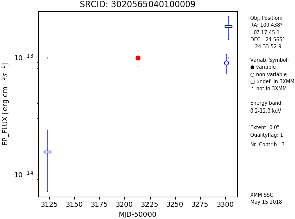
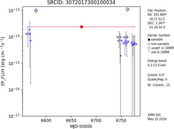
Figure 21: Example light curves of candidates for long-term variability in the stacked catalogue, produced as auxiliary catalogue products. The objects have no counterpart with SDSS classification within 5″, and their 3XMM-DR7 counterpart is not known to be short-term variable. Plot symbols inform about short- and long-term variability and non-detections in 3XMM-DR7 and are explained in Appendix B.4.

4.7 Cross-matching with the 3XMM serendipitous source catalogue DR7 and multi-wavelength catalogues

The stacked catalogue is based on a subset of 3XMM-DR7 observations. DR7s and DR7 were thus cross-matched to identify new detections from the stacks and to transfer DR7-specific information into the new resource, for example on short-term variability. To suppress false associations with spurious DR7 detections, a cleaned version of 3XMM-DR7 was created for this matching exercise. It includes all unique sources with at least one detection in an observation that was used to create the stacked catalogue and at least one detection with a good quality flag (SUM_FLAG 0 or 1). A source from the stacked catalogue and a unique source from the DR7 subset are matched if they are separated by less than 2.27 times the sum of their position errors. The factor 2.27 converts the errors from a Gaussian 68.30 % confidence region to the 99.73 % confidence region of a Rayleigh distribution, which is appropriate for coordinate errors. For the sources in the stacked catalogue, the simultaneously determined coordinates RA and DEC are used together with the pure statistical error derived from the column RADEC_ERR, and the linearly added 0.43″ component derived in Sect. 4.5. For the unique 3XMM-DR7 sources, the merged astrometrically corrected positions SC_RA and SC_DEC are used together with the combined statistical and systematic error derived from the catalogue column SC_POSERR. The matching radius per source is thus $r_{\textrm{match}}=2.27\times\left(\sigma_{\textrm{DR7,total}}+\sigma_{\textrm{stack,stat}}+\sigma_{\textrm{stack,sys.lin}}\right)$.

60 908 3XMM-DR7 counterparts of stacked sources are found and their contributing DR7 detections are identified. The associated DR7 sources are included in the stacked catalogue with their identifiers, coordinates, and short-term variability information. The combined parameters of the unique source are copied from the 3XMM-DR7 catalogue of sources to the DR7s summary row. The parameters of each contributing DR7 detection are copied from the 3XMM-DR7 catalogue of detections to the corresponding observation-level row in the stacked catalogue, if the observation was used for DR7s. This applies to a total of 114 200 individual DR7 detections of the 60 908 unique sources. The observation-level values of the DR7 associated columns remain undefined in the stacked catalogue if the DR7 source has not been detected in the respective observation. The offset between the associated DR7s and DR7 sources is given in the column DIST_3XMMDR7 in the summary rows, and the offset between the stacked source and the contributing DR7 detection in the respective observation-level row if applicable.

The parameters of associated stacked and 3XMM-DR7 sources are generally consistent with each other within a few percent, which is within their uncertainties. Sources from stacked source detection with a 3XMM-DR7 association, for example, have a median flux and median flux error of $1.98\pm 0.69\times 10^{-14}\,\textrm{erg\,cm}^{-2}\,\textrm{s}^{-1}$. The 3XMM-DR7 counterparts (unique sources) have a median flux and median flux error of $1.78\pm 0.59\times 10^{-14}\,\textrm{erg\,cm}^{-2}\,\textrm{s}^{-1}$, including sources with different numbers of contributing observations in the stacked catalogue and in 3XMM-DR7. For the detections per observation, the median values in the stacked catalogue are $2.05\pm 0.91\times 10^{-14}\,\textrm{erg\,cm}^{-2}\,\textrm{s}^{-1}$, compared to $2.08\pm 0.86\times 10^{-14}\,\textrm{erg\,cm}^{-2}\,\textrm{s}^{-1}$ in 3XMM-DR7.

Within the subset of observations that have entered the stacked catalogue, 128 509 individual detections are listed in 3XMM-DR7. About 11 % are not recovered by stacked source detection. The differences mainly lie in a higher rejection rate of spurious sources through stacked source detection (see Sects. 2.4 and 4.4), the maximum-likelihood correction scheme (Sect. 2.3), and the different background models. The percentage of low-quality detections with SUM_FLAG$>$1 among the missing DR7 sources is 30 %, significantly higher than in the complete DR7 subset ($\sim 16$%). The different background treatment and other subtleties affect the net counts of tentative sources, hence their detection likelihood and inclusion into a catalogue. For example, photons are distributed somewhat differently into pixels owing to a different spatial binning in the two catalogues compared here. This will cause fluctuations of the source content close to the detection likelihood limit. A detailed discussion on how different source-detection runs and different background values can affect the final source selection is given in Paper VII.

Of the 71 951 sources in the stacked catalogue, 11 043 do not have a counterpart in the DR7 subset and are thus new findings. The increase of the source content compares quite well with a first-order estimate based on area overlap, increased exposure time $T$ in the overlap, and an assumed $\log N-\log S$. Choosing stacks with two members only (the most abundant composition) and using $N\propto S^{-\Gamma+1}$, $S\propto T^{-0.5}$, the gain of sources through an additional exposure is $(T_{\mathrm{total}}/T_{\mathrm{part}})^{(\Gamma-1)/2}-1$. According to Mateos et al. (2008), the power-law index $\Gamma$ above and below the flux break ranges from 1.8 to 2.6 in the dominating energy bands. With a $\Gamma$ of 1.8 for sources at the sensitivity limit of XMM-Newton, the expected gain is 16 %.

When comparing the source parameters in the two catalogues, the differing methods used to derive them should be kept in mind. All values in the stacked catalogue are fitted simultaneously or directly derived from the stacked fit, while individual detections are matched to compile the 3XMM-DR7 catalogue of unique sources. In particular, the stacked source coordinates are fitted simultaneously, while the merged coordinates of the 3XMM-DR7 unique sources are weighted means of the individually fitted coordinates of the contributing detections. 3XMM-DR7 fields are astrometrically rectified by comparing them with optical and infra-red catalogues before the coordinates are merged. The values given in the RADEC_ERR columns of the stacked and the 3XMM catalogues are the statistical errors of the fit to the positions, while the merged DR7 SC_POSERR position errors include an additional component from the astrometric correction. Observations from which detections are merged into unique 3XMM-DR7 sources can be missing from the stacked catalogue because of the selection criteria of clean observations. Conversely, each selected observation in the stack is used to derive the source parameters irrespective of the detection likelihood during this observation, while a low-likelihood detection is not included in the 3XMM-DR7 catalogue and does not contribute to the merged unique source. Out of the 60 908 associated sources, only 26 356 thus have the same number of contributing observations in both catalogues, while 26 395 have more and 8 157 have fewer contributions in the stacked catalogue than in 3XMM-DR7.

The stacked catalogue has been also cross-matched with a selection of external optical and infra-red catalogues and the pre-release version of the Chandra CSC 2.0 using the X-Match service of the Centre de Données astronomiques de Strasbourg (Pineau et al. 2011). The best match within a radius of 5″ is chosen. Table 3 gives the number of matches and their percentage with respect to the stacked catalogue. 57 268 or 80 % of the sources have a tentative optical or infra-red counterpart, 59 227 one in any of the selected catalogues including CSC 2.0. To estimate the fraction of false associations, a histogram of the position offsets between the stacked catalogue and all matches in the external catalogue is produced up to 30″. For a uniform local source density, the number of all spurious matches depends linearly on the offset. This linear component dominates the offset histogram above approximately 5″ for the chosen external catalogues. From a linear fit, the number of all spurious associations within the matching radius 5″ is derived and subtracted from the number of all associations, resulting in the expected number of true associations. Its deviation from the number of best matches (first column of Table 3) gives an estimate of their spurious content and is included in the fourth column of Table 3.

Table 3: Cross-matches of the sources in the stacked catalogue: best X-match within a radius of 5″, given in total numbers in the column labelled ‘Matches’ and as percentage of the 71 951 stacked catalogue sources in the column ‘Share’. The estimated content of false associations among the matches is given in the column ‘False pos’[itives].

Catalogue	Matches	Share	False pos.	Ref.
2MASS	16 859	23.4 %	32 %	(1)
AllWISE	40 163	55.8 %	7 %	(2)
GALEX GR5 AIS	6 609	9.2 %	9 %	(3)
UKIDSS DR9 LAS	8 208	11.4 %	18 %	(4)
NOMAD	31 628	44.0 %	20 %	(5)
Pan-STARRS1	36 995	51.4 %	18 %	(6)
SDSS DR12	21 887	30.4 %	29 %	(7)
Gaia DR2	28 321	39.4 %	32 %	(8)
Chandra CSC 2.0 pre1	13 771	19.1 %	1 %	(9)

(1) Skrutskie et al. (2006); (2) Cutri & et al. (2014); (3) Bianchi et al. (2011); (4) Lawrence et al. (2007); (5) Zacharias et al. (2004); (6) Chambers et al. (2016); (7) Blanton et al. (2017); (8) Gaia Collaboration et al. (2018); (9) Evans et al. (2010).

4.8 Caveats

The following limitations to this first stacked catalogue have been identified and described throughout the paper. They are summarised in this section.

The catalogue is based on a selection of good-quality observations. In particular, repeated observations of a field have not entered the catalogue if they have been attributed a 3XMM-DR7 OBS_CLASS greater than two.

The detection likelihoods, calculated as the mathematical equivalent of a two-parameter fit, can be low if very few source counts are distributed across many images, and faint sources may be lost for purely statistical reasons. The effect is largely compensated by the refined box-detection strategy and source-selection criteria used to construct the stacked catalogue.

Although the number of spurious detections is reduced by stacked source detection with respect to the individual observations, the catalogue is not free from spurious content, for example along instrumental features, stray light, or residuals in the PSF fit to bright sources. Many of them can be identified by visual inspection of the images. A filtering expression on the total detection likelihood helps to further decrease the potentially spurious content at the expense of losing transient sources.

The source quality flags are purely derived by the automated quality assessment of a modified version of dpssflag without visual screening. They warn the users about low detector coverage of a source, possible source confusion, a source position on known bad pixels, and potential extended spurious detections. Source images published together with the catalogue offer the opportunity to inspect the detection area (see Sects. 4.9 and B.4).

No astrometric correction has been applied to the measured source positions. Their mean systematic error is estimated to be 0.43″ up to 0.74″, depending on its definition. This astrometric accuracy is better than that of the uncorrected source positions listed in the 2XMM and 3XMM catalogues.

High-proper motion objects are not uniquely recovered by stacked source detection, because the algorithm is not designed to follow position changes between observations. They show up as several seemingly long-time variable objects in the catalogue and need to be identified manually or via comparison with astrometric catalogues.

4.9 Access to the catalogue and auxiliary products

The catalogue table is compiled as one file in the Flexible Image Transport System (FITS) format and can be downloaded directly from the website of the XMM-Newton SSC. The website also provides the catalogue documentation and links to the other resources. The list of observations, also delivered in FITS format, informs about all selected OBS_IDs, their assignment to stacks, the area covered, the exposure time ratio to the longest observation in the stack, and the setup of the observation including the filters chosen per instrument. Web-based user interfaces to the catalogue and the associated auxiliary products are provided by the XCatDB and ESA’s XMM-Newton Science Archive (XSA). The catalogue is also included in the VizieR and HEASARC data services.

For all sources in the catalogue, auxiliary products are created: broad-band X-ray images in the $0.2-12.0$ keV energy band, false-colour RGB images within $0.2-1.0$ keV, $1.0-2.0$ keV, and $2.0-12.0$ keV, corresponding to the energy bands 1 plus 2, 3, and 4 plus 5, and optical finding charts from the highest-quality image out of Pan-STARRS G (Chambers et al. 2016), skyMapper G (Wolf et al. 2018), and ESO Online Digitized Sky Survey DSS2 blue and red band. All images are centred on the source position in the stacked catalogue. The X-ray and RGB images show a section of the mosaics, which are created from all observations in a stack using the task emosaic, and cover 10′ $\times$ 10′. Information on source extent and quality flag are included. The optical finding charts have a side length of 2′. For all sources that were observed at least twice with non-zero counts, long-term light curves are constructed from the mean all-EPIC fluxes in the stack and each contributing observation. Short-term variability according to 3XMM-DR7 is indicated in the plots if a counterpart has been found. Details on the long-term light curves and on the construction of the optical finding charts are given in Sect. B.4 of the Appendix. Figure 24 shows a complete set of the auxiliary products for an arbitrarily chosen source.

5 Summary and conclusions

The first serendipitous source catalogue from overlapping XMM-Newton observations, named 3XMM-DR7s, contains 71 951 unique sources in 1 789 observations, taken between 2000 and 2016 and grouped into 434 stacks. Its processing is based on a new module, using existing, improved, and new source-detection code, which is distributed as part of the XMM-Newton Science Analysis System. Stacked source detection proves to be more sensitive to faint sources and likely results in a lower false-positive rate than source detection on the individual observations. Source parameters are determined with higher accuracy, and the catalogue can be used in particular to investigate faint sources and potentially variable sources. About 15% of the sources in 3XMM-DR7s are new with respect to 3XMM-DR7. At least 60 % of them have tentative counterparts in other catalogues within 5″.

The stacked catalogue gives information on the parameters of each source in the stack of observations as well as in its contributing observations and on long-term flux variability directly from the fitting process. Post-processing quality assessment is automatically applied to all sources. An accompanying list of observations includes their technical details like the observation date and the filters used. The auxiliary source images can be accessed via the XSA interface to the stacked catalogue.

Providing information on source detection and catalogue construction, this paper is intended to be the reference for 3XMM-DR7s and subsequent releases of stacked catalogues. The future releases are envisaged to be based on less restrictive selection criteria of observations to be included in the stacks than used for this first edition. They are planned to provide upper-limit flux estimates at the source positions. Methods to apply astrometric corrections to the individual observations before performing stacked source detection will be investigated to further improve its sensitivity.

Appendix A The automated method used to identify high-background fields

To establish a high-background threshold for each EPIC instrument from a large sample of exposures, a mean background count rate per unit area between 0.2 and 12.0 keV is determined for each of the about 8 000 3XMM-DR7 EPIC observations taken in full-frame or large-window mode in the following way. From the event lists pre-filtered with the 3XMM GTIs, source-excised images are created per instrument by excluding circular regions around known 3XMM-DR7 sources with the radius being the maximum of (i) 30″, (ii) the square root of the counts as a rough approximation to PSF scaling, and (iii) – if the source has a summary flag of 0 or 1 in 3XMM-DR7 indicating a good-quality detection – the source extent. For bright sources with an EPIC/pn count rate above 1 count s^-1, summed over all five energy bands, stripes along the readout direction are excluded to get rid of out-of-time events. To simplify the procedure, the stripes have a constant width of 40″ over the whole chip extent. Corresponding source-excised masks are derived from the source-excised images, which give the valid pixels per instrument during the observation.

The averaged background count rate per area in units of cts arcsec^-2 s^-1 in each source-excised image is the total number of photons divided by the number of pixels in the source-excised mask, the pixel size in square arcseconds, and the net exposure time in seconds. For EPIC-pn, the four quadrants are treated separately, because they are independent of each other and can have different lifetimes and thus background levels, in particular if they are operated in continuous counting mode while the telemetry of the instruments is saturated and data are transmitted incompletely and unusable for scientific analyses. The maximum background value of the quadrants is used as a measure of the whole observation.

The method has two general limitations. Firstly, it does not distinguish between high sky background and emission of very extended sources within the field of view. Both scenarios are considered problematic for (stacked) source detection and treated in the same way. Secondly, background features that are prominent on small scales only like stray light are not reliably flagged by this method, since the count rate is calculated as an average over the chip or chip quadrants. A measure of spatial background variability over the field of view can be used to identify these cases and may be implemented in the future.

The distributions of mean background values are shown in Fig. 22 for each EPIC instrument. Observations that have a HIGH_BACKGROUND flag in 3XMM-DR7 are plotted in red, with a zoom to high rates in the inset. The 3XMM flag is set for the whole observation if at least one instrument experienced increased background. In the plots per instrument of Fig. 22, some observations with a low mean background level in one instrument are therefore marked in red owing to a DR7 background flag triggered by one of the other instruments. The height of the peak in the histograms is estimated from a fit with an empirically chosen Lorentz function $l(r)=h/((r-c)^{2}/w^{2}+1)$ with count rate $r$, peak centre $c$, height $h$, and half width at half maximum $w$, omitting the left wing of the peak. It translates into a cumulative Half Cauchy probability distribution $2\arctan((\log_{10}(r)-c)/w)/\pi$, regarding background count rates left of the peak as low background with probability zero. For the stacked catalogue, a probability cut of 87 % was used to exclude high-background observations from stacked source detection (Sect. 3.1).

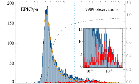
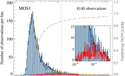
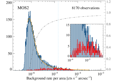
Figure 22: Histograms of the derived background rates per area of all considered observations of EPIC-pn, MOS1, and MOS2 (from top to bottom). The orange line shows the Lorentz fit to the histogram and the grey dash-dotted line the Half Cauchy probability distribution, with the scale given in the right axis. The dashed vertical line marks the 87 % probability cut used to discard observations as high-background contaminated. The red histogram shows the distribution of observations that have a HIGH_BACKGROUND flag in 3XMM-DR7 for comparison. Insets: zoom to the highest background values.

Appendix B Auxiliary information on the stacked catalogue and its selection of observations

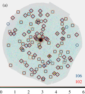
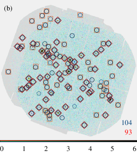
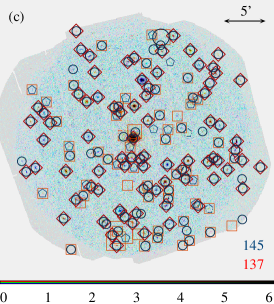
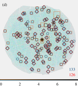
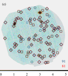
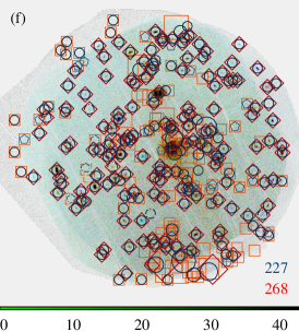
Figure 23: Example detection images of catalogue stacks and detections in the respective individual observations, including a field with considerable spurious content. As in Fig. 18, stacked detections are shown in blue and combined individual detections in red. Thick circles and diamonds mark detections that are significant in at least two observations, thin pentagons and boxes the others. Dashed symbols are used for detections that have been flagged by dpssflag. (a) Two observations with identifiers 0693662101 and 0723780201. (b) Two observations with identifiers 0203840101 and 0203840201. (c) Three observations with identifiers 0205650401, 0205650601, and 0205650701. (d) Two observations with identifiers 0674320301 and 0674320401. (e) Two observations with identifiers 0505010501 and 0505011201. (f) Five observations with identifiers 0124712501, 0204040101, 0204040301, 0304320201, and 0304320301.

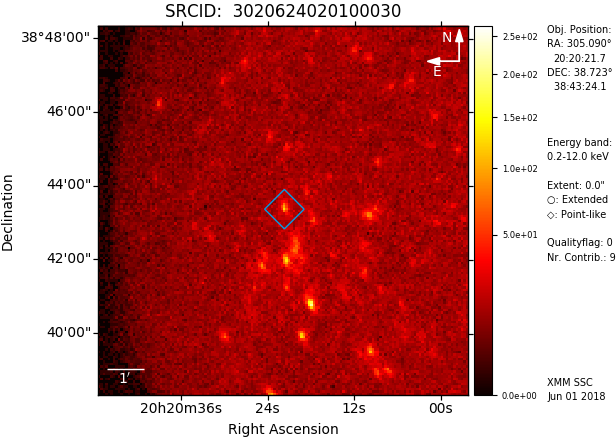
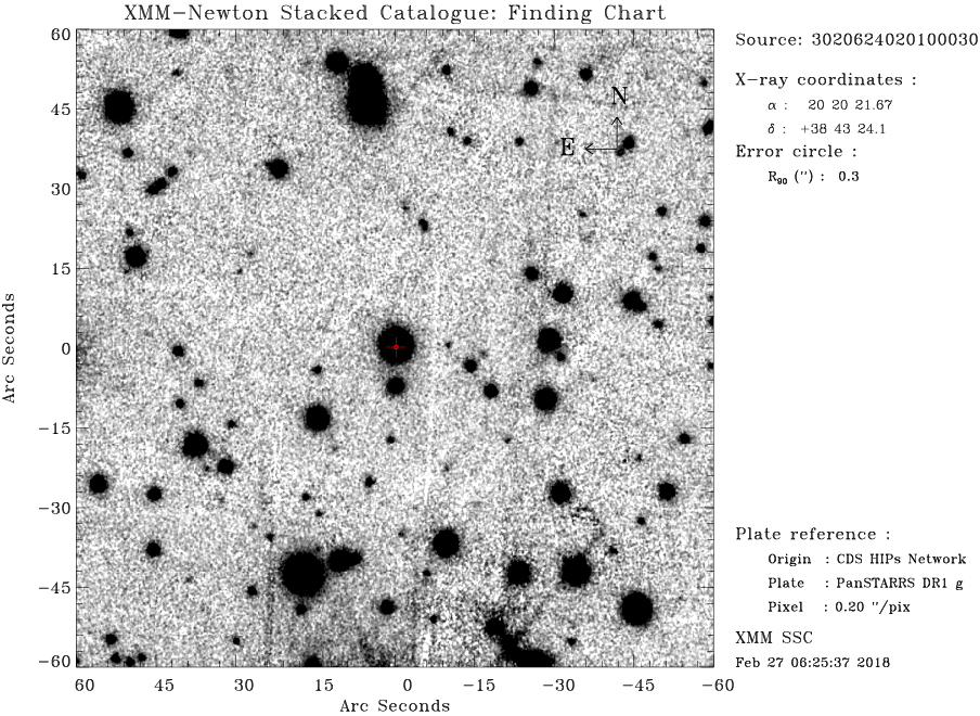
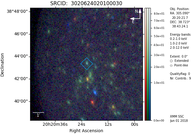
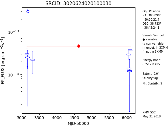
Figure 24: Examples of the auxiliary products accompanying each catalogue source: broad-band X-ray image, false-colour RGB image of three X-ray energy bands, optical finding chart, and long-term light curve.

B.1 Proposal categories included in the catalogue

Table 4 lists the number of catalogue observations per XMM-Newton proposal category. Most of the 3XMM-DR7 observations comprising objects with large extent have been de-selected from the first stacked catalogue.

B.2 Example detection images

Figure 23 shows examples of the differences between source detection on two to five stacked observations and on the individual observations (see Sect. 4.4). As for the 3XMM catalogues of unique sources, the individual detections have been joined within a matching radius of 15″.

B.3 Catalogue columns

Table LABEL:tab:columns gives an overview of all columns included in the catalogue and a short description of how the stacked parameters and the parameters per contributing observation are calculated. Entries centred within the two columns for stacked and observation-level values are valid for both of them. ‘Null’ stands for undefined values / not-a-number, ‘zero’ for 0.0. Weighted means of values $x_{i}$ with errors $\sigma_{i}$ are calculated as $\bar{x}=(\sum_{i=0}^{n}x_{i}/\sigma_{i}^{2})/\sigma_{x}^{2}$ with $\sigma_{x}^{2}=1/\sum_{i=0}^{n}\sigma_{i}^{-2}$. Values copied from the nearest 3XMM-DR7 source within a matching radius of three times the summed position errors are labelled by the suffix _3XMMDR7.

B.4 Auxiliary products

The optical finding charts have been generated in three steps using tools based on the HiPS standard (Fernique et al. 2017) initially designed by the Astronomical Data Center (CDS) of the Observatoire de Strasbourg and adopted by the Virtual Observatory. The procedure uses a large collection of multi-order coverage maps (Fernique et al. 2014) describing the sky coverage of many surveys and catalogues, which is operated by the CDS. The list of the HiPS surveys covering the position is requested from this database. The optical survey having the highest priority is selected and transmitted to an Aladin instance (Fernique et al. 2010) running behind a Tomcat server. This service gets the HiPS tiles covering the requested region from a CDS server and converts them into a FITS image. The operations are controlled by a Java client which runs an IDL task producing the PDF file lastly. The image cuts are tuned to highlight the fainter features. The IDL code is derived from the Astronomical Catalogue Data Subsystem (ACDS) task of the XMM-Newton pipeline.

The long-term light curves are created for sources with non-zero counts during at least two observations and include the stacked EPIC flux value and the EPIC fluxes during the contributing observations. Different plot symbols are used to indicate tentative short- and long-term variability. The stacked flux is plotted with a filled circle, if the variability VAR_PROB of the source fluxes to be consistent with constant flux is $1\,\%$ or lower. Probabilities of short-term variability are included in 3XMM-DR7 for detections with at least 100 counts and indicated in the long-term light curves by the plot symbols of the observation-level fluxes in the stacked catalogue. The flux is plotted with a filled circle, if a 3XMM-DR7 observation has been associated with the source in the stacked catalogue (cf. Sect. 4.7) and if its short-term variability flag VAR_FLAG_3XMMDR7 is true. Open circles are used in the opposite cases for tentatively non-variable sources. An open box of arbitrary size means that too few counts were collected during the observation to derive information on short-term variability in 3XMM-DR7, and a small dot that no DR7 detection has been associated with the source.

Figure 24 shows them for an example source detected in nine stacked observations.

Table 4: XSA proposal categories of the selected observations.

XSA proposal category		number
A	Stars, White Dwarfs and Solar System	382
B	White Dwarf Binaries, Neutron Star Binaries, Cataclysmic Variables, ULX and Black Holes	192
C	Supernovae, Supernova Remnants, Diffuse Emission, Diffuse galactic Emission and Isolated Neutron Stars	119
D	Galaxies, Galactic Surveys and X-ray Background	111
E	Galaxies, Groups of Galaxies, Clusters of Galaxies and Superclusters	229
F	Active Galactic Nuclei, Quasars, BL-Lac Objects and Tidal Disruption Events	291
G	Groups of Galaxies, Clusters of Galaxies and Superclusters	162
H	Cosmology, Extragalactic Deep Fields and Large Extragalactic Areas	303

2]

Table 5: Description of all catalogue columns. The table column ‘Stack’ comprises a short summary of how the parameter value in the summary row per stack is calculated, ‘Observation’ of the value derived for the individual contributing observation. Values per instrument are labelled by $CC$, which stands for one of PN, M1, M2. The energy bands, defined as for 3XMM, are abbreviated by $1\leq n\leq 5$ and for the hardness ratios by $1\leq i\leq 4$. Broad-band EPIC values are derived in the 0.2$-$12.0 keV range.

Column name	Format	Unit	Description	Observation	Stack
Columns 1$-$4: Detection characteristics
SRCID	long		Identifier of the detection.	Assigned to all rows per source
OBS_ID	string		XMM-Newton observation identifier.	Per observation	null
N_OBS	integer		Number of observations involved in the stack.	null	Per stack
N_CONTRIB	integer		Number of observations in which the source was fitted.	null	Per stack
Columns 5$-$15: Coordinates and associated identifier
RA	double	degrees	Right ascension (J2000).	Combined fit
DEC	double	degrees	Declination (J2000).	Combined fit
RADEC_ERR	float	arcsec	Square root of the sum of the squared 1$\sigma$ errors in X_IMA and Y_IMA $\sqrt{\sigma_{\textrm{X\_IMA}}^{2}+\sigma_{\textrm{Y\_IMA}}^{2}}$, converted to arcsec.	Combined fit
LII	double	degrees	Galactic longitude.	Combined fit
BII	double	degrees	Galactic latitude.	Combined fit
X_IMA(_ERR)	float	pixel	X coordinate within the re-binned image and its 1$\sigma$ error. Image pixels are binned to 4″ $\times$ 4″.	Combined fit
Y_IMA(_ERR)	float	pixel	Y coordinate within the re-binned image and its 1$\sigma$ error. Image pixels are binned to 4″ $\times$ 4″.	Combined fit
DIST_NN	float	arcsec	Distance to the nearest neighbouring detection.	Combined fit
IAUNAME	string		IAU name ‘3XMMs Jhhmmss.s$\pm$ddmmss’ of the source.	Assigned to all rows per source
Columns 16$-$23: 3XMM counterpart: values copied from 3XMM-DR7
IAUNAME_3XMMDR7	string		IAU name assigned to the nearest unique source in 3XMM-DR7.	Assigned to all rows per source with a 3XMM-DR7 counterpart
SRCID_3XMMDR7	long		Unique source identifier of the nearest source in 3XMM-DR7 within a correlation radius of three times the sum of the position errors. Null (undefined) if no counterpart is found.	Assigned to all rows per source with a 3XMM-DR7 counterpart
DETID_3XMMDR7	long		Identifier of the 3XMM-DR7 per-observation detection that contributes to the unique source SRCID_3XMMDR7, if existing.	Per OBS_ID	null
RA_3XMMDR7	double	degrees	Mean right ascension of the unique 3XMM-DR7 source and its contributing detections after field rectifications.	RA of DETID_3XMMDR7	SC_RA of SRCID_3XMMDR7
DEC_3XMMDR7	double	degrees	Mean declination of the unique 3XMM-DR7 source and its contributing detections after field rectifications.	DEC of DETID_3XMMDR7	SC_DEC of SRCID_3XMMDR7
POSERR_3XMMDR7	float	arcsec	Position error of the unique 3XMM-DR7 source and its contributing detections, including the error derived from the field rectification.	POSERR of DETID_3XMMDR7	SC_POSERR of SRCID_3XMMDR7
DIST_3XMMDR7	double	arcsec	Distance between the source and the nearest unique source / its contributing detection in 3XMM-DR7.	Distance to DETID_3XMMDR7	Distance to SRCID_3XMMDR7
NDETECT_3XMMDR7	integer		Number of DR7 detections N_DETECTIONS of the nearest unique source in 3XMM-DR7.	null	Of SRCID_3XMMDR7
Columns 24$-$71: Fluxes
EP_FLUX	float	erg cm-2 s-1	All-EPIC flux between 0.2 and 12 keV: dead-time corrected count rates in the entire PSF, multiplied with the respective energy conversion factors. Null (undefined) if the exposure is zero, like on chip gaps, or if the covered PSF fraction is below $15\,\%$.	Mean of the instrument fluxes weighted by the inverse squared errors
EP_FLUX_ERR	float	erg cm-2 s-1	1$\sigma$ error on EP_FLUX.	Inverse square root of the sum of inverse squared errors per instrument
EP_$n$_FLUX(_ERR)	float	erg cm-2 s-1	All-EPIC flux and 1$\sigma$ flux error in energy band $n$. Null (undefined) if the exposure is zero or if the covered PSF fraction is below $15\,\%$. Zero with non-zero errors, if no counts are detected in spite of sufficient PSF coverage.	Mean of the instrument values weighted by the inverse squared errors
$CC$_FLUX(_ERR)	float	erg cm-2 s-1	Total flux and 1$\sigma$ flux error in instrument $CC$. Null / zero as before.	Sum of fluxes and flux errors per energy band
$CC$_$n$_FLUX(_ERR)	float	erg cm-2 s-1	Flux and 1$\sigma$ flux error per instrument $CC$ and energy band $n$. Null / zero as before.	Fitted per input image	Mean of the observation-level values weighted by the exposure time
Columns 72$-$117: Count rates and count numbers
EP_RATE	float	counts s-1	All-EPIC count rate between 0.2 and 12.0 keV: background-subtracted and vignetting corrected count rate in the entire PSF. Null (undefined) if the exposure is zero or if the covered PSF fraction is below $15\,\%$. Zero with non-zero errors if no counts are detected in spite of sufficient PSF coverage.	Sum of the count rates per instrument	Mean of the observation-level rates weighted by the exposure time
EP_RATE_ERR	float	counts s-1	1$\sigma$ error on the count rate. Null (undefined) if the exposure is zero or if the covered PSF fraction is below $15\,\%$.	Square root of the quadratic sum of the errors per instrument	Combined observation-level errors weighted by the exposure time
$CC$_RATE(_ERR)	float	counts s-1	Total count rate and count-rate error in instrument $CC$. Null / zero as before.	Sum of the values per energy band	Mean of the observation-level values weighted by the exposure time
$CC$_$n$_RATE(_ERR)	float	counts s-1	Count rate and count-rate error per instrument $CC$ and energy band $n$. Null / zero as before.	Fitted per input image	Mean of the observation-level values weighted by the exposure time
EP_CTS	float	counts s-1	All-EPIC counts: background-subtracted source counts in the entire PSF. Null (undefined) if the exposure is zero or if the covered PSF fraction is below $15\,\%$.	Sum of the source counts per instrument
EP_CTS_ERR	float	counts s-1	1$\sigma$ error on the counts. Null (undefined) if the exposure is zero or if the covered PSF fraction is below $15\,\%$.	Square root of the quadratic sum of the errors per instrument
$CC$_CTS(_ERR)	float	counts s-1	Total counts and error in instrument $CC$.	Sum of the values per energy band
Columns 118$-$139: Detection and extent likelihoods
EP_DET_ML	float		Total equivalent maximum detection likelihood, normalised to two degrees of freedom.	Calculated from all valid contributing images
$CC$_DET_ML	float		Equivalent maximum detection likelihood for instrument $CC$, normalised to two degrees of freedom.	Calculated from all valid contributing images per instrument
$CC$_$n$_DET_ML	float		Equivalent maximum detection likelihood per instrument $CC$ and energy band $n$, normalised to two degrees of freedom.	Value per input image	Calculated from all valid contributing images per instrument and energy band
EXTENT	float	arcsec	Source extent radius, derived from the model source PSF convolved with a beta profile. Below an extent of 6″, it is considered unresolved and set to zero, the source is ‘point-like’.	Combined fit
EXTENT_ERR	float	arcsec	$1\sigma$ error on the source extent radius. Null (undefined) if the extent radius is below 6″.	Combined fit
EXTENT_ML	float		Likelihood that the source is extended with radius EXTENT. Null (undefined) if the source is considered point-like.	Combined fit
Columns 140$-$171: Hardness ratios
EP_HR$i$	float		Equivalent all-EPIC hardness ratios $(r_{i+1}-r_{i})/(r_{i+1}+r_{i})$ between the count rates $r$ in energy bands $i$ and $i+1$.	Mean of all active instruments
EP_HR$i$_ERR	float		$1\sigma$ error on hardness ratio EP_HR$i$.	Error propagation of the contributing values
$CC$_HR$i$(_ERR)	float		Hardness ratios $(r_{i+1}-r_{i})/(r_{i+1}+r_{i})$ between the count rates $r$ in energy bands $i$ and $i+1$ per instrument.	Per input images	Mean of the observations
Columns 172$-$233: Fit characteristics
$CC$_EXP	float	seconds	Exposure map values per instrument $CC$, including vignetting effects. The effective good exposure time is given in the ONTIME columns, described below.	Sum of the contributing images
$CC$_$n$_EXP	float	seconds	Exposure map values per instrument $CC$ and energy band.	Fitted per input image	Sum of the contributing images
$CC$_BG	float	counts px-1	Background model at the central position of the source on the CCD. Null (undefined) if the exposure map is zero and if the centre of the source is located on a bad chip area.	Sum of all contributing images
$CC$_$n$_BG	float	counts px-1	Background model in energy band $n$ at the CCD position of the source.	Sum of all valid images in energy band $n$
EP_ONTIME	float	seconds	Total good exposure time at the central position of the source on the CCD. Zero if the centre of the source is located on a bad chip area.	Maximum of the good exposure time per instrument	Sum of the maximum on-times of all observations
$CC$_ONTIME	float	seconds	Total good exposure time of instrument $CC$ at the CCD position of the source. Times are calculated by the task evselect and not vignetting corrected.	Read from the headers of the input files.	Sum of the observation-level values.
$CC$_MASKFRAC	float		Mean chip coverage in the detection mask per instrument, weighted by the point spread function of the source.	Minimum of the slightly differing values per energy band	Maximum of the observation-level values
EP_OFFAX	float	arcmin	Angular distance of the source to the boresight.	Minimum of the values per instrument.	null
$CC$_OFFAX	float	arcmin	Angular distance of the source to the boresight in instrument $CC$.	Combined fit	null
$CC$_$n$_VIG	float		Vignetting fraction in instrument $CC$ and energy band $n$ at the central position of the source.	Read from the calibration data base	null
Columns 234$-$238: Quality flags
STACK_FLAG	integer		Summarised quality flag of the detection. ‘0’ if all flags are false. ‘1’ if at least one of flags 1, 2, 3, 9 is true. ‘2’ if at least one of flags $4-8$ is true. ‘3’ if STACK_FLAG is 2 for all contributing observations.	Numeric version of EP_FLAG
EP_FLAG	string		Quality flags of the detection, automatically set and combined into a nine-characters string. A flag ‘true’ means a warning on a detection condition.	Worst flag of all instruments	Worst flag of all observations
$CC$_FLAG	string		Quality flags in instrument $CC$.	Set per input image	Worst flag of all observations
Columns 239$-$268: Inter-observation variability of sources with at least two contributing observations
VAR_CHI2	float		Reduced $\chi^{2}$ of inter-observation flux variability in all contributing observations with valid non-zero fluxes.	null	$\frac{1}{n-1}\sum_{k=1}^{n}\left(\frac{F_{k}-F_{\textrm{EPIC}}}{\sigma_{k}}\right)^{2}$
VAR_CHI2_$n$	float		Reduced $\chi^{2}$ of inter-observation flux variability in energy band $n$.	null
VAR_PROB	double		Probability that the measured flux values are consistent with constant inter-observation flux, derived from VAR_CHI2. The smaller VAR_PROB, the more likely the source shows inter-observation flux variability.	null	$\int_{\chi^{2}}^{\infty}\frac{x^{\nu/2-1}e^{-x/2}}{2^{\nu/2}\Gamma(\nu/2)}dx$
VAR_PROB_$n$	double		Probability that the measured flux values are consistent with constant inter-observation flux in energy band $n$.	null	Derived from VAR_CHI2_$n$
FRATIO	float		Ratio between highest and lowest (non-zero, non-null) mean flux in the contributing observations.	null	$F_{\textrm{max}}/F_{\textrm{min}}$
FRATIO_ERR	float		$1\sigma$ error on the flux ratio.	null	$\left(\frac{\sigma_{F\textrm{min}}^{2}}{F_{\textrm{min}}^{2}}+\frac{\sigma_{F\textrm{max}}^{2}}{F_{\textrm{max}}^{2}}\right)^{0.5}\,\frac{F_{\textrm{max}}}{F_{\textrm{min}}}$
FRATIO_$n$(_ERR)	float		Ratio between highest and lowest mean flux in energy band $n$ and its $1\sigma$ error.	null
FLUXVAR	float		Largest difference between mean all-EPIC fluxes in terms of $\sigma$.	null	$\max_{k,l\in[1,n]}\frac{|F_{k}-F_{|}|}{\sqrt{\sigma_{k}^{2}+\sigma_{l}^{2}}}$
FLUXVAR_$n$	float		Largest difference between mean all-EPIC fluxes in terms of $\sigma$ in energy band $n$.	null
Columns 269$-$273: 3XMM-DR7 intra-observation variability of sources with a DR7 light curve
CHI2PROB_3XMMDR7	double		EPIC $\chi^{2}$ probability that the time series of the nearest unique source in 3XMM-DR7 is consistent with the source having constant flux during the observation.	EP_CHI2PROB in 3XMM-DR7	SC_CHI2PROB in 3XMM-DR7: Minimum of all contributing 3XMM-DR7 observations
FVAR_3XMMDR7	double		Fractional variance of the nearest unique source in 3XMM-DR7.	FVAR in 3XMM-DR7 of the instrument with minimum CHI2PROB	SC_FVAR in 3XMM-DR7: Observation with minimum CHI2PROB
FVARERR_3XMMDR7	double		$1\sigma$ error on FVAR_3XMMDR7.	FVAR_ERR in 3XMM-DR7 of the instrument with minimum CHI2PROB	SC_FVAR_ERR in 3XMM-DR7: Observation with minimum CHI2PROB
VAR_FLAG_3XMMDR7	boolean		Variability flag of the nearest unique source in 3XMM-DR7. True if at least one exposure has CHI2PROB below $10^{-5}$.	EP_VAR_FLAG in 3XMM-DR7	SC_VAR_FLAG in 3XMM-DR7: Observation with minimum CHI2PROB
SUM_FLAG_3XMMDR7	integer		Integer representation of the quality flags of the nearest 3XMM-DR7 source from automatic and visual screening.	SUM_FLAG in 3XMM-DR7	SC_SUM_FLAG in 3XMM-DR7
Columns 274$-$284: Observation characteristics
MJD_FIRST	double	days	Modified Julian Date of the start of the observation (JD$-$2 400 000.5).	Read from the headers of the input files	First contributing observation
MJD_LAST	double	days	Modified Julian Date of the end of the observation (JD$-$2 400 000.5).	Read from the headers of the input files	Last contributing observation
PA_PNT	float	degrees	Mean position angle of the spacecraft during the observation.	File headers	null
REVOLUT	short		XMM-Newton orbit of the observation.	File headers	null
$CC$_SUBMODE	string		Observing mode of instrument $CC$.	File headers	null
$CC$_FILTER	string		Filter used during the observation.	File headers	null
URL_3XMMDR7	string		Web page of the nearest unique source in 3XMM-DR7.	Copied from 3XMM-DR7

Table 5: Continued.