An Efficient System for Subgraph Discovery

Abstract

Subgraph discovery in a single data graph—finding subsets of vertices and edges satisfying a user-specified criteria—is an essential and general graph analytics operation with a wide spectrum of applications. Depending on the criteria, subgraphs of interest may correspond to cliques of friends in social networks, interconnected entities in RDF data, or frequent patterns in protein interaction networks to name a few. Existing systems usually examine a large number of subgraphs while employing many computers and often produce an enormous result set of subgraphs. How can we enable fast discovery of only the most relevant subgraphs while minimizing the computational requirements?

We present Nuri, a general subgraph discovery system that allows users to succinctly specify subgraphs of interest and criteria for ranking them. Given such specifications, Nuri efficiently finds the $k$ most relevant subgraphs using only a single computer. It prioritizes (i.e., expands earlier than others) subgraphs that are more likely to expand into the desired subgraphs (prioritized subgraph expansion) and proactively discards irrelevant subgraphs from which the desired subgraphs cannot be constructed (pruning). Nuri can also efficiently store and retrieve a large number of subgraphs on disk without being limited by the size of main memory. We demonstrate using both real and synthetic datasets that Nuri on a single core outperforms the closest alternative distributed system consuming 40 times more computational resources by more than 2 orders of magnitude for clique discovery and 1 order of magnitude for subgraph isomorphism and pattern mining.

1 Introduction

Social networks, the World Wide Web, transportation networks and protein-protein interaction (PPI) networks are commonly modeled as graphs in which vertices represent entities, edges represent relationships between entities, and vertex/edge labels represent certain properties of the entities/relationships. Given such a graph, the problem of finding subgraphs (subsets of vertices and edges) that meet specific user-defined criteria arises in a variety of applications. For example, prominent star and clique structures of high homophily (i.e., sharing attributes) in social networks have been shown instrumental to understanding the nature of society [27, 8, 12, 31]. In the biological domain, subgraphs in a PPI network of highest gene expression disagreement across phenotypes (e.g., healthy/sick) are essential for identifying target pathways and complexes to manipulate a condition [50, 29, 37, 14, 15]. Other applications include computer network security [66, 44, 13], financial fraud detection [16, 46], and community discovery in social and collaboration networks [45, 47].

In response to the aforementioned demand, researchers have developed custom solutions for specific types of subgraph discovery problems. Examples include subgraph isomorphism search algorithms [26, 34, 23, 54] and techniques for discovering frequent subgraphs [40, 19, 1, 21], cliques [7, 59, 6, 55, 17, 10], quasi-cliques and dense subgraphs  [2], as well as communities [49, 64]. The above techniques, however, are one-off solutions for specific problems, do not provide the necessary system support for large-scale computations, and are usually difficult to use/extend for different subgraph discovery computations.

Various types of graph computations including PageRank [4] have been supported by TLV (“think like a vertex”) graph systems including Pregel [42, 11], GraphLab [38], Graph- -Chi [33], and TurboGraph [25]. These systems, which store the state of computation in the form of vertex attributes, however, are not suitable for subgraph discovery computations. The reason is that subgraphs cannot be adequately expressed as vertex attributes since the number of subgraphs grows exponentially with the size of the data graph and there is typically a many-to-many relationship between vertices and subgraphs of interest.

Different from the above, systems specifically targeted to subgraph discovery have recently been proposed [53, 48, 9]. These systems adopt subgraph exploration as the building block for subgraph discovery computations. In other words, they initially construct one-vertex (or one-edge) subgraphs and then repeatedly expand subgraphs into larger ones by adding a vertex or an edge at a time. As discussed later in this paper, however, these systems often exhibit limited performance (even when they employ a large number of servers) mainly due to the sheer number of subgraphs that they have to examine. They may also produce an overwhelmingly large result set, for example, millions of subgraphs, which cannot be easily dealt with by a human analyst.

We propose a new subgraph discovery system, called Nuri, that overcomes the above limitations. Nuri supports a variety of subgraph discovery computations (i) conveniently (as opposed to the complexity of developing custom solutions [67, 60, 65, 28, 23, 56, 41], for example, managing a large number of subgraphs that cannot fit into the main memory) via an API that enables succinct implementation of these computations and (ii) more efficiently compared to the closest existing alternative systems [53, 48, 9] by quickly finding the $k$ most relevant subgraphs according to user-provided specifications. The key advantageous features of Nuri are as follows:

Targeted Expansion. Our API allows users to specify whether or not it is adequate to expand a subgraph by adding a vertex or an edge. This feature enables Nuri to create and examine only the necessary subgraphs in contrast to Arabesque [53] which exhaustively creates subgraphs and then filters out irrelevant ones.

Prioritization. Our API allows users to assign a higher priority to subgraphs that are more likely to expand into subgraphs of interest than others (e.g., cliques that have the potential to expand into larger cliques). Given this specification, Nuri expands subgraphs with a higher priority before other subgraphs, thereby speeding up the discovery of the desired subgraphs. All of the previous subgraph discovery systems  [53, 48, 9] lack this feature and thus have inherent performance limitation.

Pruning. As soon as the result set contains $k$ entries, it becomes unnecessary to expand subgraphs whose expansions cannot lead to subgraphs that are more relevant than the $k$ entries (e.g., in the case of finding the largest cliques, cliques that can only expand into cliques of up to size 3 when the result set already contains a clique of size 4). Nuri can detect and safely discard such subgraphs according to a user specification.

Efficient Top-$\boldsymbol{k}$ Aggregate Subgraph Discovery. While some key subgraph discovery computations require grouping of subgraphs (e.g., by their patterns) and aggregation of certain properties (e.g., calculation of pattern frequency) [40, 19, 1, 21], previous subgraph discovery systems such as NScale [48] and GMiner [9] cannot support such aggregate computations. In contrast to Arabesque [53] that must expand all smaller subgraphs before any larger subgraph, Nuri can expand a group of subgraphs before other smaller subgraphs (prioritized expansion) thereby facilitating early and effective pruning.

On-Disk Subgraph Management. The number of subgraphs that Nuri manages usually grows exponentially with the size and density of the data graph and may even surpass the capacity of the main memory. Nuri has the ability to manage high-priority subgraphs in memory and low-priory subgraphs on disk in a highly efficient manner where the use of disk causes only a slight degradation in performance.

In summary, this paper presents the following contributions by us:

• two new computational models that efficiently support various top-$k$ subgraph discovery computations through prioritized subgraph expansion and pruning

• an API that allows users to easily implement diverse subgraph discovery computations (and examples demonstrating succinct implementation of representative subgraph discovery algorithms)

• design and implementation of a system, Nuri, that enables fast top-$k$ subgraph discovery just on a single computer

• in-depth analysis of experimental results which demonstrate between $1$ to $2$ orders of magnitude reduction of subgraph discovery time for our system running on a single computer, compared to the closest alternative distributed system utilizing $40$ times more computational resources.

The rest of this paper is organized as follows: Section 2 introduces example subgraph discovery computations and discusses previous systems that are most closely related to our work. Section 3 presents our computational models which enable fast subgraph discovery through prioritized subgraph expansion and pruning. Sections 4 and 5 explain our API and system architecture, respectively. Section 6 explains our evaluation results, Section 7 summarizes related work, and Section 8 concludes this paper.

2 Background

In this section, we discuss several popular subgraph discovery computations that we adopt to describe and evaluate our general system (Section 2.1). We also explain previous systems/solutions that are closely related to our work and their limitations (Section 2.2).

2.1 Subgraph Discovery Computations

Our goal is to enable efficient discovery of the most relevant subgraphs that meet user-specified criteria within a large data graph. For demonstrative purposes, we adopt the following example discovery computations:

(a) Graph with 4 vertices

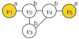
(b) Graph with 5 vertices ($a$ and $b$ are labels)

(c) Query/ pattern graph

Figure 1: Sample Graphs

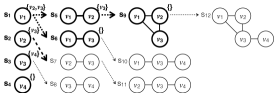
Figure 2: Clique Discovery (on the graph in Figure 1a)

Clique Discovery. A clique is a subgraph in which every pair of vertices are adjacent [7, 59, 6, 55, 17, 10]. The data graph in Figure 1a contains $9$ cliques of sizes $1$ to $3$, depicted as $s_{1}$, $s_{2}$, $s_{3}$, $s_{4}$, $s_{5}$, $s_{6}$, $s_{7}$, $s_{8}$, and $s_{9}$ in Figure 2 (details of this figure are explained in Sections 2.2 and 3.2).

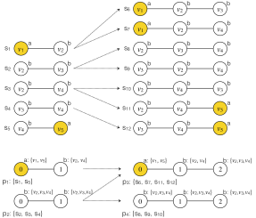
Figure 3: Pattern Mining (on the graph in Figure 1b)

Subgraph Isomorphism. The goal of subgraph isomorphism search is to find all subgraphs isomorphic to a query graph in a labeled data graph [26, 34, 23, 54]. For a query graph $G_{q}(V_{q},E_{q},L_{q})$, a subgraph $G_{s}(V_{s},E_{s},L_{s})$ in the data graph is isomorphic to the query graph if there exists a bijection $\mu:V_{q}\rightarrow V_{s}$ such that (1) $\forall{v\in V_{q}},L_{q}(v)=L_{s}(\mu(v))$ (i.e., the label of vertex $v$ in $G_{q}$ is the same as the label of the corresponding vertex $\mu(v)$ in $G_{s}$) and (2) $\forall{(v,v^{\prime})\in E_{q}}\Leftrightarrow(\mu(v),\mu(v^{\prime}))\in E_{s}$ (i.e., vertices $v$ and $v^{\prime}$ are adjacent in $G_{q}$ if and only if the corresponding vertices $\mu(v)$ and $\mu(v^{\prime})$ are adjacent in $G_{s}$). For example, the data graph in Figure 1b contains four subgraphs (depicted as $s_{6}$, $s_{7}$, $s_{11}$, and $s_{12}$ in Figure 3) that are isomorphic to the query graph in Figure 1c. Subgraph $s_{6}$ is isomorphic to the query graph since a bijection such that $\mu(0)=v_{1}$, $\mu(1)=v_{2}$, and $\mu(2)=v_{3}$ satisfies the conditions mentioned above.

Pattern Mining. The goal of pattern mining is to find subgraph patterns that appear at least as frequently as a user-specified threshold in the data graph. For example, the subgraph pattern in Figure 1c appears in the data graph from Figure 1b (the subgraphs depicted as $s_{6}$, $s_{7}$, $s_{11}$, and $s_{12}$ in Figure 3 are isomorphic to the pattern in Figure 1c).

Among several pattern frequency definitions [20, 32, 5], for the purposes of this example, we consider the minimum image-based support, which is defined as the minimum number of mappings for any vertex in the pattern to the corresponding vertices in the data graph [5]. According to this definition, the frequency of pattern $p_{1}$ in Figure 3 is 2 since (i) subgraphs $s_{1}$ and $s_{5}$ match (i.e., are isomorphic to) $p_{1}$ and (ii) the first vertex of $p_{1}$ (vertex $0$) maps to vertices $v_{1}$ and $v_{5}$ in Figure 1b, (iii) the second vertex of $p_{1}$ (vertex $1$) maps to vertices $v_{2}$ and $v_{4}$, and thus (iv) the frequency of $p_{1}$, denoted $f(p_{1})$, is $\min(|\{v_{1},v_{5}\}|,|\{v_{2},v_{4}\}|)=\min(2,2)=2$. The other patterns in Figure 3 have the following frequencies: $f(p_{2})=\min(|\{v_{2},v_{3},v_{4}\}|,|\{v_{2},v_{3},v_{4}\}|)=\min(3,3)=3$, $f(p_{3})=\min(|\{v_{1},v_{5}\}|,|\{v_{2},v_{4}\}|,|\{v_{2},v_{3},v_{4}\}|)=\min(2,2,3)=2$, and $f(p_{4})=\min(|\{v_{2},v_{3},v_{4}\}|,|\{v_{2},v_{3},v_{4}\}|,|\{v_{2},v_{3},v_{4}\}|)=\min(3,3,3)=3$.

Top-$\boldsymbol{k}$ Semantics. Given a large graph, the above computations may return an enormous number of subgraphs, thus overwhelming the user. Our goal is to allow users to specify the desired size $k$ of the result set and a criterion for ranking subgraphs. Examples include (i) the cliques of the largest size, (ii) the isomorphic matches of the highest cumulative edge weight, and (iii) the $k$ most frequent patterns of a certain size. The system then should obtain such top-$k$ results more efficiently than exhaustively acquiring all results and ranking them a posteriori.

2.2 Limitations of Current Graph Systems

Graph processing systems such as Pregel [42], Giraph [11], GraphLab [38, 22], GraphChi [33], TurboGraph [25] and others [61, 51, 52, 57, 58] adopt a “think like a vertex (TLV)” computational model. These systems iteratively update the state (i.e., variables) of each vertex in a manner that eventually computes quantities of interest, such as PageRank [4]. Subgraph discovery computations, however, cannot be succinctly expressed using vertex variables since the number of subgraphs grows exponentially with the size of the graph and there is typically a many-to-many relationship between vertices and subgraphs. For this reason, TLV systems cannot adequately support subgraph discovery computations.

In contrast to the above ones, several systems specifically targeted to subgraph discovery have recently been proposed [53, 48, 9]. These systems adopt subgraph exploration as the building block for subgraph discovery computations. In other words, they initially construct one-vertex subgraphs (e.g., $s_{1}$, $s_{2}$, $s_{3}$, and $s_{4}$ in Figure 2) or one-edge subraphs (e.g., $s_{1}$, $s_{2}$, $s_{3}$, $s_{4}$, and $s_{5}$ in Figure 3) and then expand subgraphs into larger ones by adding a vertex or an edge at a time (e.g., in Figure 3, $s_{1}$ into $s_{6}$ by adding edge $\{v_{2},v_{3}\}$).

Among the above systems, only Arabesque [53] can support pattern mining by initially constructing one-edge subgraphs and then grouping these subgraphs according to their patterns (e.g., in Figure 3, a group of subgraphs $s_{1}$ and $s_{5}$ that match pattern $p_{1}$ and another group of subgraphs $s_{2}$, $s_{3}$, and $s_{4}$ that match pattern $p_{2}$). It then computes the frequency of each pattern and repeats the process of expanding, for each pattern whose frequency is no lower than a threshold, the subgraphs that match the pattern.

The limitations of the above systems are as follows: First, as further explained in Section 3.2, they cannot perform prioritized expansion of subgraphs according to user-specified criteria, inherently losing the opportunity to quickly fill the result set and start pruning out irrelevant subgraphs whose expansions cannot affect the result set. Second, NScale [48] and GMiner [9] cannot support aggregate computations such as frequent pattern mining. Third, Arabesque [53] adopts exhaustive expansion (i.e., constructs all subgraphs that can be obtained by adding a vertex/edge to an existing subgraph) and post-expansion filtering (i.e., discards irrelevant subgraphs), and thus may create a large number of unnecessary subgraphs (e.g., non-clique subgraphs such as $s_{10}$, $s_{11}$, and $s_{12}$ in Figure 2).

Table 1: User Functions

Function	Optional	Description	Default
$expandable(s,\delta)$	yes	returns true if it is adequate to expand subgraph $s$ by adding a vertex or an edge $\delta$	returns true
$relevant(s)$	no	returns true if subgraph $s$ matches the user’s interest	N/A
$priority(s)$	yes	returns the application-specific priority of subgraph $s$	returns null
$dominated(s,s^{\prime})$	yes	returns true if all subgraphs into which $s$ can expand are guaranteed to have a lower priority than subgraph $s^{\prime}$	returns false

3 Computational Model

In this section, we explain the basic principles of our computational model (Section 3.1), its technical details (Section 3.2), and an extension to the model for supporting aggregate computations (Section 3.3).

3.1 Core Ideas

Our computational model aims to quickly find the $k$-most relevant results according to user-specified preference functions. Its key principles are as follows:

• Targeted expansion: our computational model initially creates unit subgraphs that contain a vertex (or an edge) and then obtains new subgraphs by repeatedly adding vertices and edges to existing subgraphs. It allows users to specify whether or not it is adequate to expand subgraph $s$ by adding a vertex or an edge $\delta$ (see the $expandable(s,\delta)$ function in Table 1). For example, users can avoid creation of non-clique subgraphs by making $expandable(s,\delta)$ return true only if adding $\delta$ to $s$ maintains a clique subgraph.

• Result ranking: by implementing the $relevant(s)$ function (Table 1), users can specify whether or not subgraph $s$ matches their interest (e.g., $s$ is a clique) and thus may be added to the result set. Users can also incorporate their criteria for ranking results into the $priority(s)$ function (e.g., they can express preference for larger cliques by assigning a higher priority value to larger cliques).

• Pruning: as explained in Section 3.2, it may be possible to calculate an upper bound on the priorities of all possible subgraphs into which a subgraph $s$ can expand (e.g., expansions of $s$ would only lead to cliques of size $3$ or less). In this case, users can instrument the $dominated(s,s^{\prime})$ function to return true if all supergraphs that $s$ can expand into are guaranteed to have a lower priority than $s^{\prime}$. When $s^{\prime}$ is the $k$-th entry in the result set and $dominated(s,s^{\prime})$ returns true, it is safe to ignore subgraph $s$ since expansions of $s$ can never affect the result set (i.e., all of the subgraphs obtained through these expansions would have a lower priority than $s^{\prime}$ and thus never be included in the result set).

• Prioritized expansion: our model expands highest priority subgraphs first. This feature allows users to effectively facilitate pruning by implementing the $priority(s)$ function (further details explained in Section 3.2).

The advantages of our approach compared to prior subgraph discovery systems [53, 48, 9] are discussed at the end of Sections 3.2 and 3.3.

3.2 Basic Computational Model

1 for $\textnormal{vertex}~{}v:V$ or edge $e:E$ do

2       create a subgraph $s$ containing only vertex $v$ or edge $e$;

3       insert $s$ into $Q$;

4      

5while $|Q|>0$ do

6       subgraph $s\leftarrow remove\_max(Q)$;

7       if $relevant(s)$ and

8       $~{}~{}~{}(|R|<k~{}\textnormal{{or}}~{}priority(s)\geq priority(k\textnormal{-}th(R)))$ then

9             insert $s$ into $R$;

10             if $|R|>k$ then

11                   remove from $R$ each entry $\epsilon$ such that $priority(\epsilon)<priority(k\textnormal{-}th(R))$;

12                  

13            

14      if $|R|<k~{}\textnormal{{or}}~{}!dominated(s,k\textnormal{-}th(R))$ then

15             for each neighboring vertex (or edge) $\delta$ of $s$ do

16                   if $expandable(s,\delta)$ then

17                         create subgraph $s^{\prime}$ by adding $\delta$ to $s$;

18                         if $|R|<k~{}\textnormal{{or}}~{}!dominated(s^{\prime},k\textnormal{-}th(R))$ then

19                               insert $s^{\prime}$ into $Q$;

20                              

21                        

22                  

23            

24      

25

Algorithm 1 Basic Computational Model

Algorithm 1 illustrates how our computational framework carries out subgraph discovery computations. It first creates, for each vertex (or edge) in the data graph, a subgraph $s$ containing that vertex (or edge) and inserts $s$ into a priority queue $Q$ (lines 1-3). Next, as long as $Q$ contains subgraphs (line 4), it repeatedly dequeues and processes the subgraph $s$ with the highest priority (lines 5-16). If $s$ matches the user’s interest (line 6) and if the result set $R$ is not yet full or the priority of $s$ exceeds the $k$-th entry in $R$ (line 7), it adds $s$ to $R$ (line 8) and removes unnecessary entries from $R$ (lines 9 and 10). Furthermore, it examines if subgraph $s$ can be safely ignored (i.e., unnecessary to expand $s$) (line 11). If not, it considers each neighboring vertex (or edge) $\delta$ of $s$ (line 12). If adding $\delta$ to $s$ is adequate (line 13; e.g., this expansion will lead to a clique), it expands $s$ into $s^{\prime}$ by adding $\delta$ (line 14). If $s^{\prime}$ cannot be ignored (line 15), it inserts $s^{\prime}$ into $Q$ (line 16).

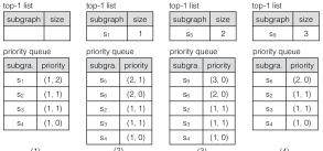
Figure 4: Maximum Clique Discovery

The following example illustrates how our computational framework can efficiently support a subgraph discovery computation by applying a classical algorithm [7].

Example: Maximum Clique Discovery. Assume that a user wants to quickly find the maximum clique(s) given a data graph in Figure 1a. For each clique $s$, the user can consider the set $P_{s}$ of vertices that may be added to $s$ while forming a clique [7] (for details of $P_{s}$, refer to Listing 1). For example, in Figure 2, $P_{s_{1}}=\{v_{2},v_{3}\}$ since clique $s_{1}$ has two neighboring vertices ($v_{2}$ and $v_{3}$) whose addition (as well as their edges to a vertex in $s$) may expand $s_{1}$ into a clique of size 3. On the other hand, $P_{s_{2}}=\{v_{3}\}$ because $s_{2}$ has only one such neighboring vertex ($v_{3}$) (note that, just like Arabesque [53], our framework does not consider adding vertex $v_{1}$ to $s_{2}$ since this expansion would result in a duplicate generation of $s_{5}$ which is to be obtained by adding vertex $v_{2}$ to $s_{1}$). The user can instrument our framework as follows (for the actual implementation of the custom functions, refer to Section 4.1):

• targeted expansion: the user can avoid creation of non-clique subgraphs by making $expandable(s,\delta)$ return true only when vertex $\delta$ is in $P_{s}$ (i.e., adding $\delta$ and its relevant edges to $s$ surely leads to a clique). In this case, every subgraph $s$ obtained through expansion is a clique (i.e., matches the user’s interest) and therefore $relevant(s)$ needs to always return true.

• prioritized expansion: the user can implement $priority(s)$ so that it returns $(|V_{s}|,|P_{s}|)$ where $V_{s}$ is the set of vertices in $s$ and $P_{s}$ is the set of vertices that may be added to $s$ while forming a larger clique. When lexicographic ordering is applied to such priority values, our framework expands larger cliques before smaller cliques and, for cliques of the same size, expands a more promising clique (i.e., clique that is likely to expand into larger cliques) before others.

• pruning: the user can enable pruning by instrumenting $dominated(s,s^{\prime})$ to return true if $|V_{s}|+|P_{s}|$ (the maximum possible size of the cliques into which $s$ can expand) is smaller than $|V_{s^{\prime}}|$ (the size of clique $s^{\prime}$).

Figure 4 illustrates how our framework can efficiently find the maximum clique ($s_{9}$ in Figure 2) given the above custom functions and the data graph from Figure 1a. Our framework first creates unit cliques $s_{1}$, $s_{2}$, $s_{3}$, and $s_{4}$ while assigning priorities to them (1). It then dequeues $s_{1}$ (i.e., the clique with the highest priority), adds $s_{1}$ to the result set, expands $s_{1}$ into $s_{5}$ and $s_{6}$, and then enqueues $s_{5}$ and $s_{6}$ (2). Next, it dequeues $s_{5}$, adds $s_{5}$ to the result set, removes $s_{1}$ from the result set, and expands $s_{5}$ into $s_{9}$ (3). Then, it dequeues $s_{9}$, and replaces $s_{5}$ in the result set with $s_{9}$ (4). At this point, $s_{2}$, $s_{3}$, $s_{4}$, and $s_{6}$ can be pruned out since they cannot expand into cliques as large as $s_{9}$.

Discussion. To the best of our knowledge, our subgraph discovery framework is the first one that supports prioritized subgraph expansion, an ability to expand more promising subgraphs (i.e., subgraphs whose expansions are more likely to quickly fill the result set with high-priority subgraphs) before others, thereby facilitating early and effective pruning. The benefits of the Nuri over prior subgraph discovery systems [53, 48, 9] which lack prioritized expansion are evident in Figures 2 and 4. For example, Arabesque [53] must expand all smaller subgraphs (e.g., all subgraphs of size 1) before any larger one (e.g., $s_{5}$), inherently limiting pruning opportunities (as opposed to ours that can expand $s_{5}$ before $s_{2}$, $s_{3}$, $s_{4}$, and $s_{6}$ and then prune out the latter subgraphs). Arabesque also has to create all subgraphs (exhaustive expansion) and then filter out irrelevant ones such as non-cliques $s_{10}$, $s_{11}$ and $s_{12}$ (post-filtering). On the other hand, our framework can prevent creation of such irrelevant subgraphs through targeted expansion.

3.3 Aggregate Computation

1

2create a new aggregator $\mathcal{G}$;

3 for $\textnormal{vertex}~{}v:V$ or edge $e:E$ do

4       create a subgraph $s$ containing only vertex $v$ or edge $e$;

5       $g\leftarrow key(s)$; // grouping key (e.g., pattern) from $s$

6       $S\leftarrow\mathcal{G}[g]$; // the subgraph group associated with $g$ in $\mathcal{G}$

7       add $s$ to $\mathcal{S}$;

8      

9for each subgraph group $\mathcal{S}$ in $\mathcal{G}$ do

10       insert $\mathcal{S}$ into $Q$;

11while $|Q|>0$ do

12       $\mathcal{S}\leftarrow remove\_max(Q)$;

13       if $relevant(\mathcal{S})$ and

14       $~{}~{}~{}(|R|<k~{}\textnormal{{or}}~{}priority(\mathcal{S})\geq priority(k\textnormal{-}th(R)))$ then

15             insert $\mathcal{S}$ into result set $R$;

16             if $|R|>k$ then

17                   remove from $R$ each entry $\epsilon$ such that $priority(\epsilon)<priority(k\textnormal{-}th(R))$;

18                  

19            

20      if $|R|<k~{}\textnormal{{or}}~{}!dominated(\mathcal{S},k\textnormal{-th}(R))$ then

21             create a new aggregator $\mathcal{G}^{\prime}$;

22             for each subgraph $s$ in $\mathcal{S}$ do

23                   for each neighboring vertex (or edge) $\delta$ of $s$ do

24                         if $expandable(s,\delta)$ then

25                               create subgraph $s^{\prime}$ by adding $\delta$ to $s$;

26                               $g^{\prime}\leftarrow key(s^{\prime})$;

27                               $\mathcal{S}^{\prime}\leftarrow\mathcal{G}^{\prime}[g^{\prime}]$;

28                               add $s^{\prime}$ to $\mathcal{S}^{\prime}$;

29                              

30                        

31                  

32            for each subgraph group $\mathcal{S}^{\prime}$ in $\mathcal{G}^{\prime}$ do

33                   if $|R|<k~{}\textnormal{{or}}~{}!dominated(\mathcal{S}^{\prime},k\textnormal{-th}(R))$ then

34                         insert $\mathcal{S}^{\prime}$ into $Q$;

35                        

36                  

37            

38      

Algorithm 2 Aggregate Computation

Some subgraph discovery computations require grouping of subgraphs and aggregation of certain properties. Consider the case of finding the $k$ most frequent patterns having two edges in the graph from Figure 1b. As illustrated in Figure 3, this computation requires the ability to group subgraphs according to a certain feature (e.g., pattern) and then obtain an aggregate value (e.g., frequency) from all of the subgraphs within each group. Algorithm 2 shows our extension to the basic computational framework (Algorithm 1) for the above case as well as other aggregate subgraph discovery computations.

The main differences of our aggregate computation framework (Algorithm 2) compared to the basic (non-aggregate) framework (Algorithm 1) are as follows:

1. A new user-specified function, $key(s)$, returns the grouping key (e.g., pattern) of subgraph $s$. Also, an aggregator $\mathcal{G}$ associates each grouping key (e.g., pattern) with the group of subgraphs having that grouping key. For a grouping key $g$, $\mathcal{G}[g]$ denotes the subgraph group for $g$ (the group of subgraphs whose grouping key is $g$).

2. Analogous to the basic (non-aggregate) framework, prioritization, insertion into the result set, and pruning of subgraph groups are specified by functions $priority(S)$, $relevant(S)$, and $dominated(S,S^{\prime})$ where $S$ and $S^{\prime}$ are subgraph groups (as opposed to subgraphs in the basic framework). As in the basic framework, $expandable(s,\delta)$ is applied to a subgraph $s$ and a vertex (or edge) $\delta$.

The steps of our aggregate computation framework (Algorithm 2) are as follows: It first constructs a new aggregator $\mathcal{G}$ (line 1) and creates, for each vertex/edge (line 2), a subgraph $s$ containing that vertex/edge (line 3), finds the grouping key $g$ of $s$ (line 4), and inserts $s$ into the subgraph group for $g$ (lines 5-6). It then inserts each subgraph group into a priority queue $Q$ (lines 7-8). Next, as long as $Q$ contains subgraph groups (line 9), it repeatedly dequeues and processes the subgraph group $S$ with the highest priority (lines 10-27). If $S$ matches the user’s interest (line 11) and if the result set $R$ is not yet full or $S$ has as high a priority as the $k$-th entry in $R$ (line 12), it adds $S$ to $R$ (line 13) and removes unnecessary entries from $R$ (lines 14 and 15). It also examines if subgraph group $S$ can be safely ignored (i.e., unnecessary to expand subgraphs in $S$) (line 16). If not, for each subgraph $s$ in $S$ (line 18), it considers each neighboring vertex/edge $\delta$ of $s$ (line 19). If adding $\delta$ to $s$ is adequate (line 20; e.g., $s$ has fewer than 2 edges), it expands $s$ into $s^{\prime}$ by adding $\delta$ (line 21), finds the grouping key $g^{\prime}$ of $s^{\prime}$ (line 22), and then inserts $s^{\prime}$ into the subgraph group for $g^{\prime}$ (lines 23 and 24). After grouping new subgraphs as above, for each subgraph group $S^{\prime}$ (line 25), it examines if $S^{\prime}$ can be ignored (line 26). If not, it inserts $S^{\prime}$ into $Q$ (line 27).

Example: Top-$\boldsymbol{k}$ Frequent Pattern Mining. Consider the problem of finding the most frequent 2-edge patterns. A user can efficiently solve this problem by implementing custom functions as follows (for the implementation of these functions, refer to Section 4.2):

• subgraph expansion: to obtain all subgraphs consisting of up to two edges, the $expandable(s,\delta)$ function needs to return true if $s$ contains less than two edges. To include 2-edge patterns in the result set, the $relevant(S)$ function needs to return true if the grouping key (i.e., the pattern) of $S$ has two edges.

• prioritized expansion: the user can implement $priority(S)$ so that it returns $(m(S),f(S))$ where $m(S)$ denotes the number of edges in the pattern associated with subgraph group $S$ and $f(S)$ denotes the frequency of that pattern. If lexicographic ordering is applied to such priority values, our framework processes larger patterns before smaller patterns, and, for patterns of the same size, processes more promising (i.e., frequent) patterns before others.

• pruning: the user can enable pruning by (i) using a pattern frequency metric with anti-monotonicity (e.g., minimum image-based support [5]), which guarantees that any super-pattern $p^{\prime}$ of $p$ cannot have a higher frequency than $p$ (i.e., $f(p^{\prime})\leq f(p)$), and (ii) by making $dominated(S,S^{\prime})$ return true if $f(S)<f(S^{\prime})$. When $S^{\prime}$ is the $k$-th entry in the result set and $dominated(S,S^{\prime})$ returns true, all subgraphs in $S$ can be safely ignored since expansions of them cannot affect the result set (due to anti-monotonicity, all subgraph patterns obtained through these expansions would have a lower frequency than the pattern associated with $S^{\prime}$).

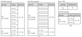
Figure 5: Most Frequent Pattern Mining

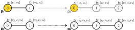
Figure 6: Relationships between Patterns

Figure 5 illustrates how our framework can efficiently find the most frequent pattern ($p_{4}$) given the above custom functions and the graph from Figure 1b. In contrast to the examples shown in Figure 3 where each subgraph expansion adds an edge to a subgraph (edge-oriented expansion) and Figure 2 where each subgraph expansion adds, to a subgraph, a vertex and its edges connected to a vertex in that subgraph (vertex-oriented expansion), this example uses a different subgraph expansion approach which we call pattern-oriented expansion.

The pattern-oriented expansion approach creates each subgraph by adding a series of directed edges and expresses each subgraph pattern using the DFS code [62]. The DFS code represents each directed edge as $(i,j,L(i),L(i,j),L(j))$, where $i$ and $j$ are vertex IDs, $L(i)$ and $L(j)$ denote the labels of vertices $i$ and $j$, and $L(i,j)$ denotes the label of the edge from $i$ to $j$ (in our examples, $L(i,j)$ are omitted since edges are not assigned any label). For example, in Figure 5, it initially creates 8 one-edge subgraphs. It obtains pattern $p_{1}$ from a subgraph containing the edge from vertex $v_{1}$ to vertex $v_{2}$ (denoted edge $v_{1}$-$v_{2}$) and another subgraph containing edge $v_{5}$-$v_{4}$. It expresses $p_{1}$ as $(0,1,a,b)$ since $p_{1}$ consists of only one edge from vertex $0$ with label $a$ to vertex $1$ with label $b$.

The pattern-oriented expansion approach constructs a subgraph $s$ only if its DFS code (i.e., the DFS code of its pattern) is minimal [62]. For example, it constructs a subgraph containing edge $v_{1}$-$v_{2}$, but not a subgraph containing edge $v_{2}$-$v_{1}$ since the DFS codes of these subgraphs are $(0,1,a,b)$ and $(0,1,b,a)$, respectively, and $(0,1,a,b)<(0,1,b,a)$. Similarly, it does not add edge $v_{4}$-$v_{5}$ to edge $v_{3}$-$v_{4}$ since the resulting DFS code $[(0,1,b,b),$ $(1,2,b,a)]$ is not minimal (adding edge $v_{4}$-$v_{3}$ to edge $v_{5}$-$v_{4}$ leads to a smaller code $[(0,1,a,b),(1,2,b,b)]$). The above subgraph construction condition provides the following guarantee:

Property 1

Let pattern $p^{\prime}$ be a super-pattern of $p$ such that the DFS codes of $p$ and $p^{\prime}$ are $[c_{1},c_{2},\cdots,c_{n-1}]$ and $[c_{1},c_{2},\cdots,c_{n}]$, respectively. Under pattern-oriented expansion, all of the subgraphs matching pattern $p^{\prime}$ can be obtained by expanding only the subgraphs matching $p$ [62].

Due to Property 1, the frequency of $p_{3}$ can be obtained by expanding only the subgraphs matching $p_{1}$ (Figure 6). On the other hand, in Figure 3 where edge-oriented expansion is applied, the frequency of $p_{3}$ can be calculated only after expanding both the subgraphs matching $p_{1}$ and the subgraphs matching $p_{2}$.

In Figure 5, our framework first forms two sugraph groups from 8 one-edge subgraphs (1). Between these groups, it selects the group for pattern $p_{2}$ (i.e., the group with the highest priority), expands the subgraphs in that group, and obtains a new group of subgraphs matching pattern $p_{4}$ (2). Since pattern $p_{4}$ has two edges (i.e., matches the user’s interest), it inserts the subgraph group for pattern $p_{4}$ in the result set (3). At this point, it can ignore the subgraphs matching pattern $p_{1}$ since the patterns obtained by expanding these subgraphs cannot be as frequent as $p_{4}$.

Discussion. To the best of our knowledge, our work mentioned above is the first top-$k$ aggregate subgraph discovery framework which supports both prioritization and pruning which can drastically improve performance (Section 6.3). Among the existing subgraph discovery systems [53, 48, 9], NScale [48] and GMiner [9] do not support aggregate computations. Arabesque [53] adopts edge-oriented subgraph expansion and thus has to expand all smaller subgraphs before any larger subgraphs (Figure 3), thereby inevitably limiting prioritization and pruning opportunities. On the other hand, due to its use of pattern-oriented expansion, our framework can quickly find each frequent pattern (e.g., $p_{4}$ in Figures 5 and 6) after expanding only one group of subgraphs matching a sub-pattern (e.g., $p_{2}$) and thus can enable early and effective pruning (e.g., pruning of subgraphs matching $p_{1}$; no creation of subgraphs matching $p_{3}$).

4 API

In this section, we present details of our API along with actual implementation code for clique discovery (Section 4.1), pattern mining (Section 4.2), and subgraph isomorphism (Section 4.3).

4.1 API for Non-Aggregate Computation

A user who wants to implement a non-aggregate subgraph discovery computation (Section 3.2) needs to choose a subgraph expansion approach between vertex-oriented expansion (Figure 2) and edge-oriented expansion (Figure 3). Then, the user needs to create a new class, in Java, that extends either the VertexOrientedSubgraph type with the expandable(Vertex v) method or the EdgeOrientedSubgraph type with expandable(Edge e) depending on the chosen expansion approach. Implementing only the relevant() method enables the most preliminary form of subgraph discovery (without result ranking, pruning, and prioritization). The user can support targeted expansion by implementing expandable(Vertex v) or expandable(Edge e), result ranking and prioritization by implementing priority(), and pruning by implementing dominated(S o), where S is a Java generic type that refers to the class being created. These methods correspond to the $expandable(s,\delta)$, $relevant(s)$, $priority(s)$, and $dominated(s,s^{\prime})$ functions in Table 1.

Listing 1: Clique Discovery (SubgraphCD)

⬇

1public HashSet<Vertex> p = null;

2

3HashSet<Vertex> p() {

4 if (p == null) {

5 p = new HashSet<Vertex>();

6 for (Vertex v : vertices())

7 if (v.equals(seed()))

8 p.addAll(neighbors(v));

9 else {

10 p.remove(v);

11 p.retainAll(neighbors(v));

12 }

13 }

14 return p;

15}

Example: Maximum Clique Discovery. As explained in Section 3.2, the maximum clique discovery computation can be implemented as follows (using a method p() that returns the set of vertices that can be added to a clique while forming a larger clique): (i) expandable(Vertex v) returns p().contains(v); (ii) relevant() returns true; (iii) dominated(S o) returns (vertexCount() + p().size() < o.vertexCount()); (iv) priority() returns new double[] { vertexCount(), p().size() }. Listing 1 shows a code snippet that implements the method p() mentioned above based on the CP algorithm [7]. For the first vertex in the current clique (line 7), it adds to a set p the neighbors of that vertex (i.e., the vertices that can be added to the clique while forming a 2-vertex clique) (line 8). For every vertex v in the current clique except the first vertex, p needs to exclude v (line 10; since v is already in that clique) and retain only the vertices connected to v (line 11; i.e., vertices that can belong to a clique containing v).

4.2 API for Aggregate Computation

Implementation of an aggregate subgraph discovery computation (Section 3.3) requires creation of two classes, one extending the SubgraphGroup type which contains the key(Subgraph s), relevant(), dominated(S o), priority() methods (corresponding to the custom functions $key(s)$, $relevant(S)$, $dominated(S,S^{\prime})$, and $priority(S)$ in Section 3.3) and another class for representing subgraphs. To enable pattern-oriented expansion (Section 3.3), the latter class must extend the PatternOrientedSubgraph type which includes the expandable(Edge e) method.

Listing 2: Pattern Mining (SubgraphGroupPM)

⬇

1Integer f = null;

2

3int f() {

4 if (f == null) {

5 MinimumImageSupport support = new MinimumImageSupport();

6 for (Subgraph s : subgraphs())

7 support.aggreagate(s);

8 f = support.frequency();

9 }

10 return f;

11}

Example: Top-$\boldsymbol{k}$ Frequent Pattern Mining. As explained in Section 3.3, for top-$k$ frequent pattern mining, the class implementing PatternOrientedSubgraph needs to include the expandable(Edge e) method which returns (edgeCount() < M). Furthermore, the class implementing the SubgraphGroup type needs to include the following methods (as shown in Listing 2, method f() returns the frequency of the pattern associated with the current subgraph group): (i) key(Subgraph s) returns pattern(s); (ii) relevant() returns (((Pattern) key()).edgeCount() == M); (iii) dominated(S o) returns (f() < o.f()); and (iv) priority() returns new double[] { ((Pattern) key()).edgeCount(), f() }.

4.3 API for Indexing

Indexing techniques for subgraph discovery typically add index entries for each vertex [23, 67]. To implement such techniques, users need to implement a class extending the Vertex type with the following methods: (i) put(k1, k2, $\cdots$, kn, v) which associates a key comprising k1, k2, $\cdots$, and kn with a value v as an attribute of the vertex, (ii) get(k1, k2, $\cdots$, kn) which returns the value associated with the key comprising k1, k2, $\cdots$, and kn, and (iii) initialize() which is invoked automatically for every vertex when the data graph is loaded into the system.

Listing 3: Subgraph Isomorphism Search (VertexIS)

⬇

1public void initialize() {

2 for (int i = 1; i <= H; i++)

3 for (Vertex n : neighbors(i)) {

4 Integer s = (Integer) get(n.label(), i);

5 put(n.label(), i, s == null ? n.get("score") :

6 Math.max(s, (Integer) n.get("score")));

7 }

8}

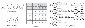
Figure 7: Subgraph Isomorphism Example

Example: Top-$\boldsymbol{k}$ Subgraph Isomorphism. Top-$k$ Subgraph Isomorphism (SI) discovery [23] aims to find, in the input graph, the $k$ highest-scored subgraphs which are isomorphic to a query graph. In this example, we define the score of each subgraph as the sum of the degree (e.g., the number of citations of each paper in a citation network) of the vertices in that subgraph. We enable targeted expansion by implementing the expandable(Edge e) method so that it returns true when the addition of e to the current subgraph leads to a larger subgraph that matches a part of the query graph (i.e., is isomorphic to a subgraph of the query graph) based on Ullman’s subgraph isomorphism algorithm [54].

To facilitate pruning in Nuri, we build an index for every vertex in the input graph in a way similar to the work by Gupta et al. [23]. The index stores, for each hop count $d$ and vertex label $l$, the maximum degree over all vertices that have label $l$ and that are $d$-hop away from the vertex under consideration (Figure 7 and Listing 3). Every subgraph also maintains a look-up map of the vertices in the query graph that are not yet matched to the vertices in that subgraph. If a subgraph is obtained by repeatedly expanding a subgraph containing a seed vertex $s$, it is possible to derive an upper bound on the scores of the subgraphs that the subgraph can expand into. This upper bound is defined as the sum of (1) the current score of the subgraph and (2) an upper bound on the score that can be obtained from the un-matched vertices in the look-up map (i.e., $\sum_{v\in\mathcal{M}}{index(s,label(v)},hop(v))$, where $\mathcal{M}$ denotes the look-up map, $hop(v)$ denotes the distance of $v$ in the query graph from the vertex that corresponds to vertex $s$, $label(v)$ denotes the label of vertex $v$, and $index(s,l,h)$ denotes the value in the index for vertex $s$, label $l$, and hop count $h$.

Figure 7 shows how the score upper bound explained above can be calculated for each subgraph. For example, subgraph $s_{2}$ contains vertex $v_{2}$ which is matched with vertex $0$ in the query graph. Therefore, its look-up map contains vertex $1$ (which is not yet matched) in the query graph. The current score of $s_{2}$ is 2 since the degree of its only vertex $v_{2}$ is 2. Vertex $1$ in the look-up map is 1 hop away from vertex 0 and its label is $a$. Since the maximum degree over all vertices in the data graph that has label $a$ and is 1 hop away from vertex $v_{2}$ is 2 (see the index in Figure 7), without expanding $s_{2}$ to include vertex $v_{3}$, it can be found that an additional score of 2 can be obtained from vertex $1$ in the look-up map. Therefore, the score upper bound for $s_{2}$ is calculated as 4. Similarly, the score upper bound for $s_{1}$, $s_{3}$, and $s_{4}$ are calculated as 3, 4, and 3, respectively. Furthermore, subgraph $s_{2}$ has a higher priority (i.e., upper bound) than $s_{1}$, and thus $s_{2}$ is expanded earlier than $s_{1}$. In the case of top-1 subgraph isomorphism discovery, $s_{1}$ can be safely discarded after $s_{2}$ is expanded into $s_{6}$ whose final score is 4. The reason is that any subgraph expanded from $s_{1}$ can only have a lower score than $s_{6}$. To support pruning and prioritization as explained above, dominated(S o) and priority() need to return (score() + u() < o.score()) and new double[] { edgeCount(), score() + u() }, where score() and u() return the score and the score upper bound of the current subgraph, respectively.

5 System Architecture

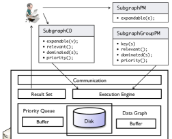
Figure 8: System Architecture

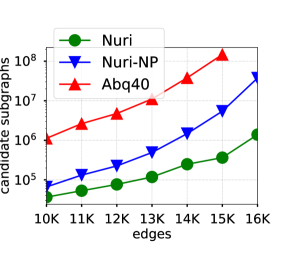
(a) subgraphs

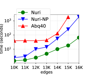
(b) time

Figure 9: Clique Discovery (Email)

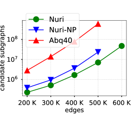
(a) subgraphs

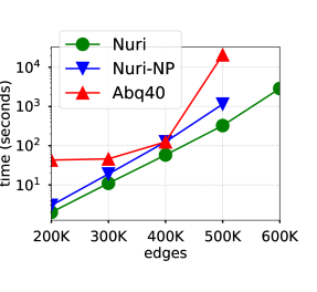
(b) time

Figure 10: Clique Discovery (MiCo)

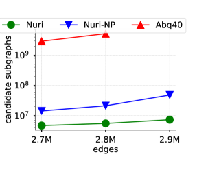
(a) subgraphs

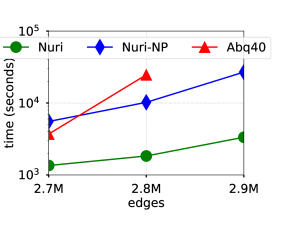
(b) time

Figure 11: Clique Discovery (YouTube)

Figure 8 illustrates the architecture of our system. When a user submits an implementation of non-aggregate subgraph discovery (e.g., SubgraphCD for clique discovery), the execution engine carries out the computation by inserting unit subgraphs into the priority queue and repeats the process of dequeuing the subgraph with the highest priority and expanding it into larger subgraphs while inserting the subgraphs matching the user’s interest into the result set and pruning out irrelevant subgraphs (Algorithm 1). When a user submits an implementation of aggregate subgraph discovery (e.g., SubgraphPM and SubgraphGroupPM for pattern mining), the execution engine carries out additional grouping and aggregation operations (Algorithm  2). For each subgraph discovery computation, the execution engine loads the data graph from the disk into the main memory. When each computation completes, the obtained result set is sent to the user. The communication component enables such interactions between the user and the system.

The number of subgraphs kept in the priority queue usually increases exponentially with the size and density of the data graph. For this reason, we created an implementation of external priority queue that can store a large number of entries on disk without being limited by the size of the main memory [18].

Our implementation, called virtual priority queue, has the ability to manage high-priority subgraphs in memory and low-priory subgraphs on disk in a highly efficient manner where the use of disk causes only a slight degradation in the speed of enqueue/dequeue operations (Section 6.6). It initially maintains subgraphs using a standard memory-resident priority queue. Whenever the memory usage becomes higher than a threshold, it retains only half of the subgraphs in the memory-resident queue and stores the others on disk in order of decreasing priority. The collection of the subgraphs on disk is called a run (analogous to runs in the context of external sorting [43, 39]). When there are multiple runs (since the memory-resident queue was full multiple times in the past), it can still quickly retrieve subgraphs from all of the runs in order of decreasing priority (analogous to external merge sort [43, 39]). It also applies buffering to read each run with a small number of disk seeks.

6 Evaluation

In this section, we explain our setup (Section 6.1) for evaluating the effectiveness of Nuri in comparison to alternatives for clique discovery (CD), pattern mining (PM), and subgraph isomorphism (SI) computations (Sections 6.2, 6.3, and 6.4). We also discuss the impact of the result set size ($k$) on subgraph discovery computations (Section 6.5) and the performance of our virtual priority queue implementation (Section 6.6).

6.1 Experimental setup

Table 2: Datasets

	$|V|$	$|E|$	distinct labels
Email [35]	986	16k	-
CiteSeer [63]	3.3k	4.5k	6
MiCo [63]	100k	1.1m	29
YouTube [64]	1.1m	2.9m	-
Patents [24]	2.7m	14m	37

Datasets. We employ five graph datasets from diverse domains and at different scales as shown in Table 2. Vertices in the Email dataset represent people and each edge between two vertices indicates that at least one email message was sent between the people corresponding to the vertices. The CiteSeer dataset represents a citation network in which each publication is labeled by its research area. The MiCo dataset expresses a co-authorship network where authors are labeled by their research interests and a pair of authors is connected if they co-authored at least one publication. The YouTube and Patents datasets represent a social network among the users of the service and a citation network among the US patents for the period between $1963$ to $1999$. In the Patents dataset, each vertex is labeled by the year in which the patent was granted.

Systems Compared. We compare two versions of our system, Nuri (supporting targeted expansion, pruning, and prioritization) and Nuri-NP (supporting only targeted expansion), and Arabesque [53] as a representative of the prior subgraph discovery systems [53, 48, 9]. In contrast to NScale [48] and GMiner [9], Arabesque supports aggregate subgraph discovery (e.g., pattern mining) and its implementation is openly available.

Both Nuri and Nuri-NP are implemented as single-threaded Java programs using the standard Java $8$ distribution. In our experiments, each of these versions was run on a single core at 1.90GHz of an Intel(R) Xeon(R) E5-4640 server ($256GB$ memory) running Red Hat Enterprise Linux Server release $7.5$. In contrast, Arabesque was executed on a total of $40$ cores from $5$ Intel(R) Xeon(R) E5430 servers (each with $8$ cores at 2.66GHz and $16GB$ memory), benefiting from its distributed computing capability. In this section, the results obtained from Arabesque are labeled “Abq40”.

Evaluation Metrics. We quantify the performance of both Nuri and Arabesque by the following metrics: (1) number of candidate subgraphs: Both Arabesque and Nuri examine candidate subgraphs obtained through expansion until the desired result is obtained. Hence, we consider the number of candidate subgraphs as the basic cost unit, allowing us to represent the inherent computational load without being affected by implementation details (e.g., specific data structures used to represent subgraphs and the actual implementation code for grouping subgraphs according to their patterns). (2) completion time of subgraph discovery: This metric allows us to compare different systems/techniques from the user’s point of view. It also compensates for the limitation of the first metric, which cannot incorporate the overhead for optimization (e.g., time spent for prioritizing subgraphs and evaluating pruning conditions). In addition, it allows us to take into account Arabesque’s ability to speed up subgraph discovery through distributed computing.

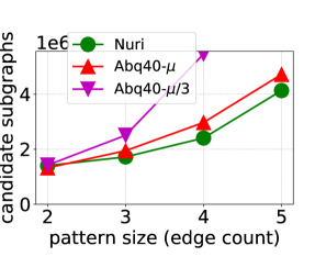
(a) subgraphs

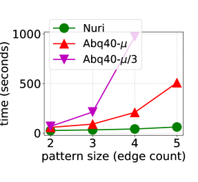
(b) time

Figure 12: Pattern Mining (Patents)

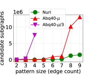
(a) subgraphs

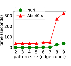
(b) time

Figure 13: Pattern Mining (CiteSeer)

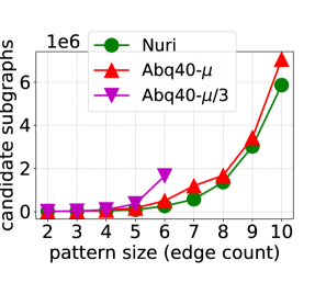
(a) subgraphs

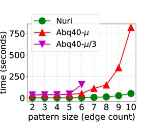
(b) time

Figure 14: Pattern Mining (MiCo)

6.2 Clique Discovery Evaluation

To obtain clique discovery (CD) results from Arabesque, we instrumented it to find all cliques and then select the largest clique(s) among them. We created increasingly denser data graphs using the Email, MiCo, and Youtube datasets by repeatedly adding batches of randomly chosen edges to an empty graph. Denser graphs tend to include more and larger cliques, increasing the complexity of clique discovery.

Figures 11,  11, and  11 show the CD results obtained for the three datasets. As expected, both the number of candidate subgraphs and completion time increase with the density of the data graph for all of the systems. In Figure 11, the gap between Nuri-NP and Abq40 is due to the advantage of targeted expansion, which allows Nuri to explore only relevant subgraphs (cliques). On the other hand, Arabesque exhaustively creates subgraphs and then filters out irrelevant (non-clique) subgraphs. The difference between Nuri-NP and Nuri demonstrates that Nuri can safely ignore a large number of candidate subgraphs (pruning) benefiting from prioritization (for $16k$ edges, Nuri examines only $1/26$ of subgraphs and is $29$x faster compared to Nuri-NP). It is also evident that the benefits of pruning and prioritization increase with density. In contrast to Nuri, Arabesque must find all smaller subgraphs before any larger subgraph (no pruning/prioritization). As a result, for data graphs with $15k$ edges, Nuri can find the largest clique(s) by examining only a small fraction (about $1/400$) of subgraphs compared to Arabesque, resulting in $2$ orders of magnitude improvement in running time although Nuri is given much less computing resources ($1$ core vs. $40$ cores). For $16k$ edges, Nuri completes the computation within $2$ minutes while Arabesque cannot within $10$ hours.

Figures 11 and 11 show the CD results obtained for the MiCo and YouTube datasets. Given $500k$ edges from the MiCo dataset, Nuri examines only $1/85$ of subgraphs compared to Arabesque (Figure 10a), resulting in a $65$x improvement in running time (Figure  10b). On $600k$ edges from the MiCo dataset, neither Arabesque nor Nuri (without pruning and prioritization) finish their computation within $10$ hours whereas Nuri (with pruning and prioritization) completes within $47$ minutes. Given $2.8M$ edges from the YouTube dataset, compared to Arabesque, Nuri examines $2$ orders of magnitude fewer candidate subgraphs (Figure  11a) and is 1 order of magnitude faster (Figure 11b). When $2.9M$ edges are used, Arabesque does not complete within $10$ hours while Nuri finishes in less than $1$ hour.

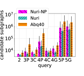
(a) subgraphs

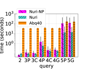
(b) time

Figure 15: SI (CiteSeer)

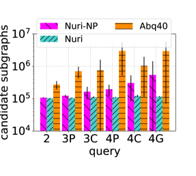
(a) subgraphs

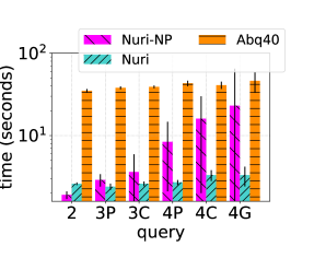
(b) time

Figure 16: SI (MiCo)

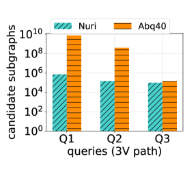
(a) subgraphs

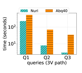
(b) time

Figure 17: Impact of Selectivity

6.3 Pattern Mining Evaluation

Our pattern mining (PM) implementation finds, given a number $M$, the most frequent patterns of size $M$ (i.e., $M$-edge patterns) in the data graph (Listing 2). To obtain the same result, we instrumented Arabesque to (1) find all of the $M$-edge patterns whose frequency is no lower than a threshold $T$ and then (2) select the most frequent one(s) among these patterns. This Arabesque implementation has the benefit of proactively pruning out (i.e., not expanding) subgraphs whose pattern has a frequency lower than $T$ (due to anti-monotonicity [5], expansions of these subgraphs cannot lead to the $M$-edge patterns whose frequency is at least $T$). In real-world use cases, however, it is difficult to appropriately set $T$ for Arabesque since the maximum frequency (denoted $\mu$) over patterns of size $M$ is not known in advance. If $T$ is set to a value greater than $\mu$, Arabesque cannot report any patterns of size $M$ since all of the patterns of size $M$ have a frequency lower than $T$. If $T$ is assigned a value lower than $\mu$, it examines subgraphs that are unnecessary for the purpose of finding the most frequent pattern(s).

Figure 14 shows the PM result obtained for the Patents dataset. When the threshold $T$ for Arabesque is set to $\mu$, Nuri and Arabesque explore a similar number of subgraphs (Nuri and Abq40-$\mu$ in Figure 12a). The difference in the number of subgraphs between these systems is due to their use of different expansion approaches (Section 3.3). In Figure 12b, the gap between Nuri and Abq40-$\mu$ shows the benefits of pattern-oriented expansion (Nuri) over edge-oriented expansion (Arabesque). Under pattern-oriented expansion (Section 3.3), when subgraph $s$ expands into $s^{\prime}$, the pattern of $s^{\prime}$ can be quickly obtained by appending only one edge to the pattern of $s$ (incremental pattern generation). On the other hand, under edge-oriented expansion, the pattern of each subgraph is always computed from scratch by converting that subgraph into its canonical form with high overhead [53]. When the threshold $T$ for Arabesque is set to $\mu/3$, Arabesque examines subgraphs unnecessary for the purpose of finding the most frequent patterns, in contrast to Nuri which automatically prunes out such subgraphs. For $M=4$ and $T=\mu/3$, Arabesque explores 2.5x more subgraphs than Nuri (Figure 12a). For $M=5$ and $T=\mu/3$, Arabesque does not complete its operation as its memory requirement surpasses the capacity of the system.

Similar trends for PM can be seen for the CiteSeer and MiCo datasets (Figures 14 and 14, respectively). In these datasets, only a few distinct labels are assigned to vertices, which allows an enormous number of subgraphs to match the same pattern (i.e., very high computational overhead). For this reason, we introduced synthetic labels, increasing the number of labels from $6$ to $48$ in CiteSeer and from $29$ to $87$ in MiCo (i.e., reduced computational overhead). In Figures 14 and 14, Arabesque explores much more subgraphs compared to Nuri, incurring substantially higher overhead. The benefits of Nuri over Arabesque (pruning and prioritization) become more evident as the pattern size increases. When $T$ is set to $\mu/3$, Arabesque does not complete due to its high memory demand when the pattern size is 4 for CiteSeer and 6 for MiCo.

6.4 Subgraph Isomorphism Evaluation

Our top-$k$ subgraph isomorphism (SI) implementation discovers, in the data graph, the $k$ highest-scored subgraphs that are isomorphic to a given query graph, where the score of each subgraph is defined as the sum of the degree of the vertices in that subgraph (Section 4.3). This implementation adopts Ullman’s algorithm [54] to efficiently find the subgraphs that match the query graph (targeted expansion). Since Arabesque [53] does not support targeted expansion, our SI implementation for Arabesque exhaustively explores subgraphs while filtering out subgraphs that do not pass a subgraph isomorphism test (a user-provided implementation). We also extended Arabesque so that it can maintain the $k$ highest-scored subgraphs.

To conduct SI computations, we pre-computed query graphs of sizes from 2 to 5 by running a sampling algorithm [36] on each data graph constructed from the CiteSeer and MiCo datasets. For 4-vertex subgraphs, we considered three different types (path, clique, and general that are labeled “4P”, “4C”, and “4G”). We also considered these three types for 5-vertex subgraphs. Since $3$-vertex subgraphs can only form a clique or a path, we did not include the general subgraph type. For 2-vertex subgraphs, we considered only one type (labeled “2”) which corresponds to both the clique and path types. For each type of query graph, we carried out SI computations using 10 query graphs (i.e., samples) and then calculated the mean values for the number of subgraphs and completion time. The graph from CiteSeer is small and sparse and thus contains very few cliques of size $5$. Therefore, we did not consider cliques of size 5.

To facilitate pruning and prioritization, our SI implementation uses an index computed for every vertex in the data graph up to $d$-hops, where $d$ is the maximum diameter of all query graphs. The index construction time for $4$-hops (sufficient for query graphs of up to size 5) was $1$ second for CiteSeer dataset. For the MiCo dataset, due to the size and the high density of the dataset, the index construction time for $3$-hops took $300$ minutes using a single core. Index construction (which is needed only once for multiple SI computations), however, is highly parallelizable because the computation for each vertex can be done independently. The index construction time was reduced to $600$ seconds when $32$ cores of a server were used.

As evident in Figures 15a and 16a, as the query graph size increases, both Arabesque and Nuri explore more subgraphs for each query type. In the CiteSeer graph, due to the sparsity of the graph, clique queries are very selective and in general explore a smaller number of subgraphs than path/general subgraph queries of the same size. The selectivity of queries also depends on the frequency of the query labels in the data graph, which affects the number of candidate subgraphs generated in the systems. In Figures 15a and 16a, the difference between Nuri-NP and Abq40 demonstrates the benefits of targeted expansion. Figures 15b and 16b show that Nuri is substantially faster than Arabesque taking advantage of pruning, prioritization, and targeted expansion even when it runs on a single core and Arabesque runs on a total of $40$ cores.

Figure 17 illustrates how the selectivity of query graphs affects the SI computation for the CiteSeer dataset. In the figure, Q1 is a non-selective query for which several million matches exist in the data graph. Q2 is a mildly selective query and Q3 is a highly selective query with fewer than $400$ matches in the data graph. Figure 17a shows that Nuri explores $4$ orders of magnitude fewer subgraphs than Arabesque for the non-selective query (Q1) due to prioritization and pruning and thus runs faster than Arabesque (Figure 17b) despite using only 1/40 of computational resources compared to Arabesque. Figure 17a also shows that as the selectivity of query increases (Q2 and Q3), the benefits of prioritization and pruning diminish since fewer subgraphs in the data graph match the query graph. In Figure 17b, Arabesque’s time costs for Q2 and Q3 are mostly caused by its distributed operation (particularly, coordination of multiple workers) rather than actual exploration of subgraphs.

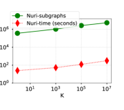
(a) CD (Email)

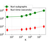
(b) PM (CiteSeer)

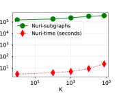
(c) SI (CiteSeer)

Figure 18: Effect of Result Set Size ($k$)

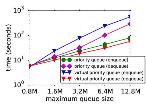
Figure 19: Virtual Priority Queue Result

6.5 Effect of the Result Set Size ($\boldsymbol{k}$)

The previous evaluations focused on top-$1$ computations. As the result set size ($k$) increases, Nuri tends to explore more subgraphs since it can start pruning out subgraphs only after its result set contains $k$ entries (i.e., as the result set needs to include more entries, Nuri can prune out fewer subgraphs). We measured the effect of $k$ on the number of candidate subgraphs examined by Nuri as well as the overall time spent for subgraph discovery computations. In this evaluation, we performed clique discovery on the Email dataset and pattern mining and subgraph isomorphism computations on the CiteSeer dataset. In Figure 19, as long as $k$ is smaller than $1000$, both the number of candidate subgraphs and running time vary insignificantly. When $k$ is greater than $1000$, the number of candidate subgraphs and running time increase modestly with $k$.

6.6 Performance of Virtual Priority Queue

We measured the performance of our virtual priority queue (Section 5) while configuring it to store subgraphs on an HGST Travelstar 2.5-Inch 1TB 5400RPM SATA 6Gbps 8MB Cache internal hard drive. To carry out the measurement solely focusing on the enqueue and dequeue costs without being affected by individual subgraph computations, we first enqueued a certain number (0.8M, 1.6M, 3.2M, 6.4M, and 12.8M) of distinct 10-edge subgraphs (growing phase) and then dequeued all of them (shrinking phase). In Figure 19, curves labeled “priority queue (enqueue)” and “priority queue (dequeue)” show the duration of the growing and shrinking phases, respectively, when Java’s standard priority queue implementation (PriorityQueue) was used (up to 40GB of memory was required). Curves labeled “virtual priority queue (enqueue)” and “virtual priority queue (dequeue)” show the time results when our virtual priority queue used at most 3GB of memory while storing on disk subgraphs that were not able to fit into the memory.

The above results show that, compared to PriorityQueue which manages all of the subgraphs in memory incurring much higher memory overheard, our virtual priority queue performs quite competitively (time costs are at most 1.8 times higher when both the growing and shrinking phases are considered, at most 7 times higher during the growing phase, and as low as 19% of PriorityQueue’s dequeue cost during the shrinking phase). The reason for our virtual priority queue’s high enqueue and low dequeue costs is that it creates sorted runs during the growing phase (paying relatively high costs) and then significantly benefits from these sorted runs during the dequeue phase.

7 Related Work

This section summarizes related work focusing on top-$k$ subgraph discovery and top-$k$ query processing. Other closely related work, particularly subgraph discovery computations as well as previous graph processing and subgraph discovery systems are extensively discussed in Sections 2.1 and 2.2, respectively.

Maximum Clique Discovery. Our maximum clique discovery implementation (Sections 3.2 and 4.1) is based on the CP algorithm [7] which calculates, for each clique $s$, an upper bound on the size of the cliques that $s$ can expand into and then prunes out $s$ if its size upper bound is smaller than the size of largest clique(s) discovered. Researchers have also developed algorithms that can more efficiently find maximum cliques by finding a tighter upper bound than CP [6, 55, 17, 10]. We leave the implementation of these algorithms for Nuri as our future work.

Top-$\boldsymbol{k}$ Pattern Mining. Given a single large graph, Grami [40] finds the patterns in the graph that are as frequent as the given threshold without ranking the patterns based on their frequency. While our top-$k$ pattern mining implementation finds the $k$ most frequent patterns of a certain size (Sections 3.3 and 4.2), the closest work that we are aware of [19] finds the $k$ largest patterns that are as frequent as a given threshold.

Top-$\boldsymbol{k}$ Subgraph Isomorphism. Our top-$k$ subgraph isomorphism implementation is motivated by Gupta et al.’s work [23] which uses an index to quickly identify subgraphs whose expansions cannot produce any of the desired subgraphs (i.e., $k$ highest-scored subgraphs that match a query graph). Zou et al. developed another solution that uses a different indexing approach [67]. We intend to implement and evaluate this solution for Nuri.

Custom Top-$\boldsymbol{k}$ Subgraph Discovery. There are also subgraph discovery techniques that are designed to quickly obtain the $k$ subgraphs of highest preference according to a user-specified criterion [60, 65, 28, 56, 23, 41, 3]. Our future work includes implementation of these techniques for Nuri.

Top-$\boldsymbol{k}$ Query Processing. In the context of database systems, various techniques for top-$k$ queries have been developed [30]. These techniques commonly maintain (1) a top-$k$ result set, from which a threshold (the lowest-priority item in the set) is obtained, and (2) an upper bound on the priorities of unexamined data items. If the threshold is higher than the upper bound (i.e., none of the unexamined data items can be included in the result set), the result set is returned as the final answer. The top-$k$ query processing techniques for database systems cannot adequately support subgraph discovery computations since they are mainly designed for queries on relations rather than a large collection of subgraphs that need to be expanded according to their priorities.

8 Conclusions

We presented Nuri, a new system for efficient top-$k$ subgraph discovery in large graphs. Nuri’s API allows users to specify application-specific criteria for exploring and prioritizing subgraphs. Nuri’s execution proceeds by creating unit subgraphs containing a vertex or an edge, and then efficiently discovering the result set by selectively expanding subgraphs according to their priority (prioritized expansion). It also proactively discards subgraphs from which the desired subgraphs cannot be obtained (pruning). For discovery computations with high space overhead, it provides efficient on-disk management of subgraphs.

We evaluated Nuri on real-world datasets of various sizes for three example computations: maximum clique discovery, subgraph isomorphism search, and pattern mining. Nuri consistently outperformed the closest state-of-the-art alternative, achieving at least $2$ orders of magnitude improvement for clique discovery and $1$ order of magnitude improvement for subgraph isomorphism search and pattern mining, while utilizing $1/40$ of the computational resources compared to the closest alternative.

References

- [1] P. Anchuri, M. J. Zaki, O. Barkol, S. Golan, and M. Shamy. Approximate Graph Mining with Label Costs. In the 19th ACM SIGKDD International Conference on Knowledge Discovery and Data Mining (KDD), pages 518–526, 2013.
- [2] R. Andersen. A Local Algorithm for Finding Dense Subgraphs. In Proceedings of the Nineteenth Annual ACM-SIAM Symposium on Discrete Algorithms (SODA), pages 1003–1009, Philadelphia, PA, USA, 2008. Society for Industrial and Applied Mathematics.
- [3] P. Bogdanov, B. Baumer, P. Basu, A. Bar-Noy, and A. Singh. As Strong As the Weakest Link: Mining Diverse Cliques in Weighted Graphs, volume 8188. Springer, 2013.
- [4] S. Brin and L. Page. The Anatomy of a Large-Scale Hypertextual Web Search Engine. Computer Networks and ISDN Systems, 30:107–117, 1998.
- [5] B. Bringmann and S. Nijssen. What Is Frequent in a Single Graph? In The Pacific-Asia Conference on Knowledge Discovery and Data Mining, pages 858–863, 2008.
- [6] C. Bron and J. Kerbosch. Finding All Cliques of an Undirected Graph (Algorithm 457). Communications of the (ACM), 16(9):575–576, 1973.
- [7] R. Carraghan and P. M. Pardalos. An Exact Algorithm for the Maximum Clique Problem. Operations Research Letters, 9:375–382, 1990.
- [8] M. Chau and J. Xu. Mining Communities and Their Relationships in Blogs: A Study of Online Hate Groups. International Journal of Human-Computer Studies, 65(1):57–70, 2007.
- [9] H. Chen, M. Liu, Y. Zhao, X. Yan, D. Yan, and J. Cheng. G-miner: an efficient task-oriented graph mining system. In Proceedings of the Thirteenth EuroSys Conference, page 32. ACM, 2018.
- [10] J. Cheng, L. Zhu, Y. Ke, and S. Chu. Fast Algorithms for Maximal Clique Enumeration with Limited Memory. In the 18th ACM SIGKDD International Conference on Knowledge Discovery and Data Mining (KDD), pages 1240–1248, 2012.
- [11] A. Ching. Giraph: Large-scale Graph Processing Infrastructure on Hadoop. In Proceedings of the Hadoop Summit, 2011.
- [12] T. Coffman, S. Greenblatt, and S. Marcus. Graph-based Technologies for Intelligence Analysis. Communications of the ACM, 47(3):45–47, 2004.
- [13] B. Coskun, S. Dietrich, and N. Memon. Friends of An Enemy: Identifying Local Members of Peer-to-peer Botnets Using Mutual Contacts. In Proceedings of the 26th Annual Computer Security Applications Conference, pages 131–140. ACM, 2010.
- [14] X.-H. Dang, A. K. Singh, P. Bogdanov, H. You, and B. Hsu. Discriminative Subnetworks with Regularized Spectral Learning for Global-State Network Data. In T. Calders, F. Esposito, E. Hüllermeier, and R. Meo, editors, Machine Learning and Knowledge Discovery in Databases, volume 8724 of Lecture Notes in Computer Science, pages 290–306. Springer Berlin Heidelberg, 2014.
- [15] X. H. Dang, H. You, P. Bogdanov, and A. K. Singh. Learning Predictive Substructures with Regularization for Network Data. In 2015 IEEE International Conference on Data Mining (ICDM), pages 81–90, 2015.
- [16] W. Eberle, J. Graves, and L. Holder. Insider Threat Detection Using a Graph-based Approach. Journal of Applied Security Research, 6(1):32–81, 2010.
- [17] D. Eppstein and D. Strash. Listing All Maximal Cliques in Large Sparse Real-World Graphs. In Experimental Algorithms - 10th International Symposium, SEA, pages 364–375, 2011.
- [18] R. Fadel, K. V. Jakobsen, J. Katajainen, and J. Teuhola. Heaps and heapsort on secondary storage. Theoretical Computer Science, 220(2):345–362, 1999.
- [19] Z. Feida, Q. Qu, D. Lo, X. Yan, J. Han, and P. S. Yu. Mining Top-k Large Structural Patterns in A Massive Network. Proceedings of the VLDB Endowment 2011 (PVLDB), 4(11):807–818, 2011.
- [20] M. Fiedler and C. Borgelt. Subgraph Support in a Single Large Graph. In Workshops Proceedings of the 7th IEEE International Conference on Data Mining (ICDM), pages 399–404, 2007.
- [21] M. R. Garey and D. S. Johnson. Computers and Intractability: A Guide to the Theory of NP-Completeness. W. H. Freeman, 2002.
- [22] J. E. Gonzalez, Y. Low, H. Gu, D. Bickson, and C. Guestrin. PowerGraph: Distributed Graph-Parallel Computation on Natural Graphs. In 10th USENIX Symposium on Operating Systems Design and Implementation (OSDI), pages 17–30, 2012.
- [23] M. Gupta, J. Gao, X. Yan, H. Cam, and J. Han. Top-K Interesting Subgraph Discovery in Information Networks. In Proceedings of the 30th International Conference on Data Engineering (ICDE), 2014.
- [24] B. H. Hall, A. B. Jaffe, and M. Trajtenberg. The NBER Patent Citation Data File: Lessons, Insights and Methodological Tools. http://www.nber.org/patents/, 2011.
- [25] W. Han, S. Lee, K. Park, J. Lee, M. Kim, J. Kim, and H. Yu. TurboGraph: A Fast Parallel Graph Engine Handling Billion-scale Graphs in a Single PC. In the 19th ACM SIGKDD International Conference on Knowledge Discovery and Data Mining (KDD), pages 77–85, 2013.
- [26] W.-S. Han, J. Lee, and J.-H. Lee. Turboiso :Towards Ultrafast and Robust Subgraph Isomorphism Search in Large Graph Databases. VLDB Endowment, pages 517–528, 2014.
- [27] L. Holder, D. Cook, J. Coble, and M. Mukherjee. Graph-based Relational Learning with Application to Security. Fundamenta Informaticae, 66(1-2):83–101, 2005.
- [28] L. Hong, L. Zou, X. Lian, and S. Y. Philip. Subgraph Matching with Set Similarity in A Large Graph Database. IEEE Transactions on Knowledge and Data Engineering, 27(9):2507–2521, 2015.
- [29] H. Hu, X. Yan, Y. Huang, J. Han, and X. J. Zhou. Mining Coherent Dense Subgraphs Across Massive Biological Networks for Functional Discovery. Bioinformatics, 21(suppl 1):i213–i221, 2005.
- [30] I. F. Ilyas, G. Beskales, and M. A. Soliman. A Survey of Top-k Query Processing Techniques in Relational Database Systems. ACM Comput. Surv., 40(4):11:1–11:58, 2008.
- [31] C. Jiang, F. Coenen, and M. Zito. A Survey of Frequent Subgraph Mining Algorithms. The Knowledge Engineering Review, 28(01):75–105, 2013.
- [32] M. Kuramochi and G. Karypis. Finding Frequent Patterns in a Large Sparse Graph. dmkd, 11(3):243–271, 2005.
- [33] A. Kyrola, G. E. Blelloch, and C. Guestrin. GraphChi: Large-Scale Graph Computation on Just a PC. In 10th USENIX Symposium on Operating Systems Design and Implementation (OSDI), pages 31–46, 2012.
- [34] J. Lee, R. Kasperovics, W.-S. Han, and J.-H. Lee. An In-depth Comparison of Subgraph Isomorphism Algorithms in Graph Databases. Proceedings of the VLDB Endowment 2012 (PVLDB), pages 133–144, 2012.
- [35] J. Leskovec, J. Kleinberg, and C. Faloutsos. Graph evolution: Densification and shrinking diameters. ACM Transactions on Knowledge Discovery from Data (TKDD), 1(1):2, 2007.
- [36] R.-H. Li, J. X. Yu, L. Qin, R. Mao, and T. Jin. On Random Walk Based Graph Sampling. In Proceedings of the 31st International Conference on Data Engineering (ICDE), pages 927–938, 2015.
- [37] X. Li, M. Wu, C.-K. Kwoh, and S.-K. Ng. Computational approaches for detecting protein complexes from protein interaction networks: a survey. BMC genomics, 11(1):S3, 2010.
- [38] Y. Low, J. Gonzalez, A. Kyrola, D. Bickson, C. Guestrin, and J. M. Hellerstein. GraphLab: A New Framework For Parallel Machine Learning. In Proceedings of the Twenty-Sixth Conference on Uncertainty in Artificial Intelligence (UAI), pages 340–349, 2010.
- [39] L. S. Lozinskii. An Analysis of External Merge Sorting Techniques. Cybernetics, 4(1):25–35, 1968.
- [40] E. M., A. E., S. S., and K. P. Grami : Frequent Subgraph and Pattern Mining in a Single Large Graph. Proceedings of the VLDB Endowment 2014 (PVLDB), pages 517–528, 2014.
- [41] K. Macropol, , and A. Singh. Scalable Discovery of Best Clusters on Large Graphs. In Proceedings of the VLDB Endowment, pages 693–702. VLDB, 2010.
- [42] G. Malewicz, M. H. Austern, A. J. C. Bik, J. C. Dehnert, I. Horn, N. Leiser, and G. Czajkowski. Pregel: A System for Large-Scale Graph Processing. In Proceedings of the 2010 ACM SIGMOD International Conference on Management of Data (SIGMOD), pages 135–146, 2010.
- [43] H. H. Manker. Multiphase Sorting. Communications of the (ACM), 6(5):214–217, 1963.
- [44] S. Nagaraja, P. Mittal, C.-Y. Hong, M. Caesar, and N. Borisov. BotGrep: Finding P2P Bots with Structured Graph Analysis. In USENIX Security Symposium, pages 95–110, 2010.
- [45] S. Papadopoulos, Y. Kompatsiaris, A. Vakali, and P. Spyridonos. Community Detection in Social Media. Data Mining and Knowledge Discovery, 24(3):515–554, 2012.
- [46] C. Phua, V. Lee, K. Smith, and R. Gayler. A Comprehensive Survey of Data Mining-based Fraud Detection Research. arXiv preprint arXiv:1009.6119, 2010.
- [47] M. Plantié and M. Crampes. Survey on Social Community Detection. In Social media retrieval, pages 65–85. Springer, 2013.
- [48] A. Quamar, A. Deshpande, and J. Lin. Nscale: neighborhood-centric analytics on large graphs. Proceedings of the VLDB Endowment, 7(13):1673–1676, 2014.
- [49] U. N. Raghavan, R. Albert, and S. Kumara. Near Linear Time Algorithm to Detect Community Structures in Large-scale Networks. Physical review E, 76(3):036106, 2007.
- [50] S. Ranu, M. Hoang, and A. Singh. Mining Discriminative Subgraphs from Global-state Networks. In Proceedings of the 19th ACM SIGKDD international conference on Knowledge discovery and data mining, pages 509–517. ACM, 2013.
- [51] S. Salihoglu and J. Widom. GPS: A Graph Processing System. In Conference on Scientific and Statistical Database Management (SSDBM), pages 22:1–22:12, 2013.
- [52] B. Shao, H. Wang, and Y. Li. Trinity: A Distributed Graph Engine on a Memory Cloud. In Proceedings of the 2013 ACM SIGMOD International Conference on Management of Data (SIGMOD), pages 505–516, 2013.
- [53] C. H. C. Teixeira, A. J. Fonseca, M. Serafini, G. Siganos, M. J. Zaki, and A. Aboulnaga. Arabesque: A System for Distributed Graph Mining. In Proceedings of the 25th Symposium on Operating Systems Principles (SOSP), pages 425–440, 2015.
- [54] J. R. Ullmann. An Algorithm for Subgraph Isomorphism. J. ACM, 23(1):31–42, 1976.
- [55] T. Uno. MACE: Maximal Clique Enumerator, ver 2.0. http://research.nii.ac.jp/~uno/code/mace.html.
- [56] E. Vasilyeva, M. Thiele, C. Bornhövd, and W. Lehner. Top-k Differential Queries in Graph Databases. In East European Conference on Advances in Databases and Information Systems, pages 112–125. Springer, 2014.
- [57] K. Wang, G. H. Xu, Z. Su, and Y. D. Liu. GraphQ: Graph Query Processing with Abstraction Refinement - Scalable and Programmable Analytics over Very Large Graphs on a Single PC. In 2015 Annual Technical Conference, USENIX (ATC), pages 387–401, 2015.
- [58] Z. Wang, Y. Gu, Y. Bao, G. Yu, and J. X. Yu. Hybrid Pulling/Pushing for I/O-Efficient Distributed and Iterative Graph Computing. In Proceedings of the 2016 ACM SIGMOD International Conference on Management of Data (SIGMOD), pages 479–494, 2016.
- [59] Q. Wu and J. Hao. A Review on Algorithms for Maximum Clique Problems. European Journal of Operational Research, 242(3):693–709, 2015.
- [60] Y. Wu, S. Yang, and X. Yan. Ontology-based Subgraph Querying. In Data Engineering (ICDE), 2013 IEEE 29th International Conference on, pages 697–708. IEEE, 2013.
- [61] R. S. Xin, J. E. Gonzalez, M. J. Franklin, and I. Stoica. GraphX: A Resilient Distributed Graph System on Spark. In First International Workshop on Graph Data Management Experiences and Systems (GRADES), page 2, 2013.
- [62] X. Yan and J. Han. gSpan: Graph-Based Substructure Pattern Mining. In Proceedings of the IEEE International Conference on Data Mining (ICDM), pages 721–724, 2002.
- [63] X. Yan, P. S. Yu, and J. Han. Graph Indexing: A Frequent Structure-based Approach. In Proceedings of the 2004 ACM SIGMOD international conference on Management of data, pages 335–346. ACM, 2004.
- [64] J. Yang and J. Leskovec. Defining and Evaluating Network Communities Based on Ground-truth. Knowledge and Information Systems, 42(1):181–213, 2015.
- [65] S. Yang, F. Han, Y. Wu, and X. Yan. Fast Top-k Search in Knowledge Graphs. In Data Engineering (ICDE), 2016 IEEE 32nd International Conference on, pages 990–1001. IEEE, 2016.
- [66] Y. Zhao, Y. Xie, F. Yu, Q. Ke, Y. Yu, Y. Chen, and E. Gillum. BotGraph: Large Scale Spamming Botnet Detection. In NSDI, volume 9, pages 321–334, 2009.
- [67] L. Zou, L. Chen, and Y. Lu. Top-k Subgraph Matching Query in A Large Graph. In Proceedings of the ACM first Ph. D. workshop in CIKM, pages 139–146. ACM, 2007.