Classical correspondence of the exceptional points in the finite non-Hermitian system

Abstract

We systematically study the topology of the exceptional point (EP) in the finite non-Hermitian system. Based on the concrete form of the Berry connection, we demonstrate that the exceptional line (EL), at which the eigenstates coalesce, can act as a vortex filament. The direction of the EL can be identified by the corresponding Berry curvature. In this context, such a correspondence makes the topology of the EL clear at a glance. As an example, we apply this finding to the non-Hermitian Rice-Mele (RM) model, the non-Hermiticity of which arises from the staggered on-site complex potential. The boundary ELs are topological, but the non-boundary ELs are not. Each non-boundary EL corresponds to two critical momenta that make opposite contributions to the Berry connection. Therefore, the Berry connection of the many-particle quantum state can have classical correspondence, which is determined merely by the boundary ELs. Furthermore, the non-zero Berry phase, which experiences a closed path in the parameter space, is dependent on how the curve surrounds the boundary EL. This also provides an alternative way to investigate the topology of the EP and its physical correspondence in a finite non-Hermitian system.

I Introduction

If a quantum system is conservative, a cyclic adiabatic change in a parameter space, in which the wave function of the system follows instantaneous eigenstates, can often give rise to surprising results such as the emergence of gauge-invariant Berry phases Berry . Of particular interest is the case where eigenvalue degeneracies are enclosed within the parameter loop. In the Hermitian regime, the corresponding Berry phase is always the real number Xiao . Over the past decades, there has been intense interest in the complex Berry phase acquired during the adiabatic evolution in the non-Hermitian systems Garrison ; Dattoli ; Ning ; Moore ; Gao ; Pont ; Massar ; Ge ; Whitney ; Dehnavi ; Nesterov ; Cui ; Liang ; ZXZ , which arises naturally in connection with various experiments. The Berry phase generalized to non-Hermitian systems provides a geometrical description of the quantum evolution of non-Hermitian systems Dehnavi and give the relationship between the geometric phase and the quantum phase transition Nesterov ; ZXZ .

Another intriguing feature is the topology of the Berry phase, which has gained considerable attention in the topological band theoryThouless ; Kane ; Moore2007 ; FuPRL ; FuPRB ; Schnyder ; Kitaev2009 ; Bansil ; Chiu ; Armitage . Topological insulators can be classified in the light of discrete symmetries and dimensionality Chiu . Topological properties of one-dimensional (1D) systems with periodical boundary condition are characterized by the so-called Zak phase, i.e., the Berry phase picked up by a particle moving across the whole Brillouin zone Zak . The Zak phase is closely related to the electric polarization in solids and plays a key role in the modern theory of insulators Xiao ; Resta . Most of those studies focus on the Hermitian system. However, particle gain and loss are generally present in natural systems that can be described by non-Hermitian Hamiltonians Moiseyev . This stimulates a growing interest in topological properties of non-Hermitian Hamiltonians Hu ; Esaki ; TonyPRL ; Leykam ; Duan ; Chong ; Xiong . Interestingly, non-Hermitian systems compared with Hermitian ones exhibit highly nontrivial characteristics. A fascinating example is non-Hermitian Hamiltonians at exceptional points (EPs), where two (or more) eigenfunctions collapse into one so the eigenspace no longer forms a complete basis. Most recently, the topological nature of EPs in non-Hermitian Hamiltonians with chiral symmetry has been recognized TonyPRL ; Leykam and the dynamical phenomena near the EPs are being investigated both theoretically Uzdin ; Berry2011 ; Berry2013 ; Gilary ; Graefe ; Moiseyev2014 ; Milburn and experimentally Moiseyev2016 ; Harris .

Most of previous studies concentrated on the non-Hermitian many-particle systems with continuous momentum, which requires the dimension of the system to be infinite. The topology of such non-Hermitian systems can be characterized by the modified Zak phase TonyPRL , which is associated with the bulk-boundary correspondence. For the finite non-Hermitian many-particle systems, however, few studies have been done on the topological properties of EP. Thus, a natural question to ask is whether the finite non-Hermitian many-particle system has obvious topological properties. These motivate us to study the topology of the EP in the finite non-Hermitian many-particle system. To this end, we systematically study the topology of the EPs in a simple $2\times 2$ non-Hermitian system and then apply the conclusion to the non-Hermitian Rice-Mele (RM) model that can be realized in experiment. Based on the analytical solution, we show that the Berry connection of the EL is connected to the curl field induced by the vortex filament. This feature is protected by the chiral symmetry of the system. In this point of view, the exceptional line (EL) directly corresponds to the vortex filament. Therefore, the topology of the EL is straightforward. Specifically speaking, when the system parameters are varied so as to form a closed loop enclosing an EL in the parameter space, the accumulated Berry phase is limited to an integer multiples of $\pi/2$, which depends on how the trajectory encircles the EL. This is topological since it occurs only if the loop encloses the EL irrespective of its precise shape. Furthermore, the Berry phase of the many-particle quantum state in the finite non-Hermitian system is merely determined by the boundary EL. When the dimension of the system increases to infinite, the Berry phase should be taken as a multiples of $\pi$ since the trajectory cannot surround a single EL. These also pave the way to investigate the topology of the EP and its physical correspondence in a finite non-Hermitian system.

The remainder of the paper is organized as follows. In Section II, we establish a bridge between the EL of non-Hermitian systems and the classical electromagnetics. In Section III, we apply the classical correspondence to investigate the topology of the non-Hermitian RM model. Finally, we give a summary and discussion in Section IV.

II Classical correspondence of the topological invariant

We start our analysis from a $2\times 2$ matrix consisting of pauli operators,

$$H=\alpha\sigma_{x}+\left(\beta+i\gamma\right)\sigma_{y},$$ (1)

where $\alpha$, $\beta$, and $\gamma$ are real numbers. The nonhermiticity of this matrix arises from the complex coefficients of the Pauli operator $\sigma_{y}$. This non-Hermitian Hamiltonian containing all the information of the system not only can be employed to describe the optical systems with gain or loss but also serve as the core matrix in the non-Hermitian lattice system. It is worth pointing out that the Hamiltonian (1) can be constructed through an arbitrary combination of the two Pauli operators. For simplicity, we confine the discussion to the Hamiltonians with $\sigma_{x}$ and $\sigma_{y}$. The following main conclusion is still hold for any possible combinations of two Pauli operators.

The eigenenergies of the system under consideration take the form $\pm\varepsilon$, where

$$\varepsilon=\sqrt{\alpha^{2}+\left(\beta+i\gamma\right)^{2}}.$$ (2)

The two eigenenergies are complex owing to the existence of $i\gamma$. When $\beta=0$, and $\gamma=\pm\alpha$, this system exhibits an EP at the square-root branch point, where the two eigenstates coalesce and one of them becomes defective. Here we refer to the two straight lines $\gamma=\pm\alpha$ as ELs. The eigenstates of Hamiltonian $H$ can construct a complete set of biorthogonal bases except the EP, which is associated with the eigenstates of its Hermitian conjugate. For the considered system, eigenstates $\left|\psi_{\pm}\right\rangle$ of $H$ and $\left|\phi_{\pm}\right\rangle$ of $H^{{\dagger}}$ form the biorthogonal bases and are explicitly expressed as

$$\left|\psi_{\pm}\right\rangle=\frac{1}{\sqrt{2}\varepsilon}\left(\begin{array}[]{c}\alpha-i\beta+\gamma\\ \pm\varepsilon\end{array}\right),\text{ }\left|\phi_{\pm}\right\rangle=\frac{1}{\sqrt{2}\varepsilon^{\ast}}\left(\begin{array}[]{c}\alpha-i\beta-\gamma\\ \pm\varepsilon^{\ast}\end{array}\right).$$ (3)

Now we focus on the symmetry of the system. The chiral symmetry of the system admits that $\left\{\sigma_{z},H\right\}=0$. So if $H$ has an eigenstate $\left|\psi_{+}\right\rangle$ with eigenenergy $\varepsilon$, then $\sigma_{z}\left|\psi_{+}\right\rangle$ is also an eigenstate with eigenenergy $-\varepsilon$.

To capture the basic property of the dynamics around the EP, we start with an adiabatic evolution, in which an initial eigenstate evolves into the instantaneous eigenstate of the time-dependent Hamiltonian. For the sake of simplicity, we assume that the Hamiltonian (1) is a periodic function of system parameters $\left\{\beta,\gamma,\alpha\right\}$ that vary with time $t$. Considering the cyclic time-dependent Hamiltonian $H\left(\beta\left(t\right),\gamma\left(t\right),\alpha\left(t\right)\right)$, it will return back to $H\left(\beta\left(0\right),\gamma\left(0\right),\alpha\left(0\right)\right)$ if all the parameters change adiabatically to the starting point after time $\tau$. The adiabatic evolution of the initial eigenstate $\left|\psi_{\pm}\right\rangle$, which follows a closed path $C$ in the $\beta-\gamma-\alpha$ parameter space, generates a Berry phase as

$$\gamma_{B}=\int_{C}\overrightarrow{\mathcal{A}}\cdot\text{d}\overrightarrow{l}\text{,}$$ (4)

where $\overrightarrow{l}$ parametrizes the cyclic adiabatic process and the Berry connection $\overrightarrow{\mathcal{A}}=\left(\mathcal{A}_{\beta},\text{ }\mathcal{A}_{\gamma},\text{ }\mathcal{A}_{\alpha}\right)$ can be expressed as

$$\mathcal{A}_{g}=i\left\langle\phi_{\pm}\left(t\right)\right|\frac{\partial}{\partial g}\left|\psi_{\pm}\left(t\right)\right\rangle,$$ (5)

where $\left|\psi_{\pm}\left(t\right)\right\rangle$ and $\left|\phi_{\pm}\left(t\right)\right\rangle$ represent the instantaneous eigenstates of the Hamiltonian $H\left(\beta\left(t\right),\gamma\left(t\right),\alpha\left(t\right)\right)$ and $H^{{\dagger}}\left(\beta\left(t\right),\gamma\left(t\right),\alpha\left(t\right)\right)$, respectively. $g=\beta$, $\gamma$, $\alpha$ denote the three directions in the parameter space. It is worth pointing out that the chiral symmetry give rise to the identical Berry connections for the eigenstates $\left|\psi_{\pm}\left(t\right)\right\rangle$, namely leads to $\mathcal{A}_{g}=\mathcal{A}_{g}^{\pm}$. After straightforward algebras, the Berry connection can be expressed as

$$\overrightarrow{\mathcal{A}}=\left(\alpha,\text{ }i\alpha,\text{ }-\beta-i\gamma\right)/\mathcal{D}$$ (6)

with $\mathcal{D}=2\varepsilon^{2}$. To demonstrate the physical correspondence of the Berry connection, we first assume that the EL can act as a vortex filament. The corresponding curl field according to the Bio-Savart law can be written as

$$\overrightarrow{A}_{\pm} = \left(-\gamma\pm\alpha,\text{ }\beta,\text{ }\mp\beta\right)/4D_{\mp},$$ (7)

$$D_{\pm} = \left(\gamma\pm\alpha\right)^{2}+\beta^{2},$$ (8)

where $\overrightarrow{A}_{\pm}$ represent the curl fields induced by the two stright vortex filaments locating at $\gamma=\pm\alpha$, respectively. Interestingly, the Berry connection and the curl field induced by the vortex filaments can be connected through the gauge transformation

$$\overrightarrow{\mathcal{A}}=\sum_{\sigma=\pm}\sigma\overrightarrow{A}_{\sigma}+\frac{i}{8}\ln\nabla\left(\frac{D_{-}}{D_{+}}\right).$$ (9)

Here $\nabla$ is the nabla operator

$$\nabla=\left(\overrightarrow{e}_{\beta}\frac{\partial}{\partial\beta},\text{ }\overrightarrow{e}_{\gamma}\frac{\partial}{\partial\gamma},\text{ }\overrightarrow{e}_{\alpha}\frac{\partial}{\partial\alpha}\right).$$ (10)

In a closed path, the second term of the Eq. (9) contributes nothing to the Berry phase. Consequently, we deem the EL as a vortex filament and sketch its direction in Fig. 1. The quantity $\gamma_{B}$ is quantized in terms of classical physics and can be treated as a topological invariant to characterize EL in the parameter space. The value of $\gamma_{B}$ depends on the loop $C$ in the $\beta-\gamma-\alpha$ parameter space: $\gamma_{B}$ is non-zero if the loop encircles an EL, while must be zero if the loop does not encircle the EL. Such a correspondence establishes a bridge between the EL of non-Hermitian systems and the vortex filament of classical physics.

Figure 1: (Color online) Schematic illustration of the classical correspondence of the ELs. The two straight red lines denote the ELs of the non-Hermitian system $H$, which can act as the vortex filaments owing to the Eq. (9).

Here we point out that the aforementioned topological invariant of the system may relate to the chiral symmetry, and this association does not rely on the system parameters. $\left\{\beta,\text{ }\gamma,\text{ }\alpha\right\}$. In fact, if one consider the following Hamiltonian

$$H^{\prime}=\mathcal{U}H\mathcal{U}^{-1},$$ (11)

where $\mathcal{U=}e^{-i\left(\overrightarrow{n}\cdot\overrightarrow{\sigma}\right)\theta/2}$ is a spin rotation operator and is independent of the system parameters $\left\{\beta,\gamma,\alpha\right\}$. Even though the new Hamiltonian $H^{\prime}$ consists of three Pauli operators, its eigenenergies are identical with those of $H$. This also indicates that the two systems possess the same EL in the parameter space. Moreover, we can redefine a chiral symmetric operator $\sigma_{z}^{\prime}=\mathcal{U}\sigma_{z}\mathcal{U}^{-1}$ to anticommute with $H^{\prime}$, i.e, $\left\{\sigma_{z}^{\prime},H^{\prime}\right\}=0$. Note that the new chiral operator is also independent of the system parameters $\left\{\beta,\gamma,\alpha\right\}$, which guarantees the identical Berry connection of the two systems

$$\mathcal{A}_{g}^{\prime}=i\left\langle\phi_{\pm}\left(t\right)\right|\mathcal{U}^{-1}\frac{\partial}{\partial g}\mathcal{U}\left|\psi_{\pm}\left(t\right)\right\rangle=\mathcal{A}_{g}.$$ (12)

Thus all the conclusion about the considered system $H$ can be applied to $H^{\prime}$. In the following section we will apply this correspondence to a finite non-Hermitian lattice system.

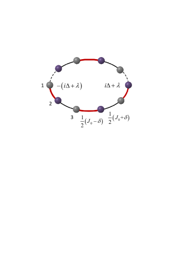
Figure 2: (Color online) Schematic illustration of extended RM model with complex on-site staggered potential. The red and black lines represent the non-uniform hopping amplitudes. The purple and gray circles denote the complex on-site staggered potentials with opposite values, respectively. The system reduced to the standard Hermitian RM model when $\Delta=0$. Note that the considered non-Hermitian system possesses the periodical boundary condition, i.e., $c_{j}\equiv c_{j+2N}$, which is crucial to diagonalize the Hamiltonian (13).

III Classical correspondence in a finte non-Hermitian lattice system

III.1 Model Hamiltonian and solution

As an example, we consider a non-Hermitian extended RM model, which can be described by the following Hamiltonian

$$\mathcal{H} = \frac{1}{2}\sum_{j=1}^{N}\left[\left(J_{0}-\delta\right)c_{2j-1}^{\dagger}c_{2j}+\left(J_{0}+\delta\right)c_{2j}^{\dagger}c_{2j+1}+\text{H.c.}\right]$$ (13)

$$+\left(i\Delta+\lambda\right)\sum_{j=1}^{2N}\left(-1\right)^{j}c_{j}^{\dagger}c_{j}\text{,}$$

the non-Hermiticity of which arises from the on-site staggered complex potential $\left(i\Delta+\lambda\right)\sum_{j=1}^{2N}\left(-1\right)^{j}c_{j}^{\dagger}c_{j}$. The system possesses a $2N$-site lattice, where $c_{j}$ is the annihilation operator of a fermion on site $j$. The nominal tunneling strength $J_{0}$ is staggered by $\delta$. For clarity, we sketch the structure of the system in Fig. 2. The origin Hermitian Hamiltonian with $\Delta=0$ can be realized with controlled defects using a system of attractive ultracold fermions Chin ; Strohmaier ; Hacke in a simple shaken one-dimensional optical lattice. Furthermore, the non-Hermitian version can be achieved in a zigzag array of optical waveguides with alternating optical gain and loss Longhi . It is worth mentioning that this non-Hermitian Hamiltonian can be also utilized to control the wavepacket dynamics HWH ; Lin . Now we consider the periodical boundary condition, that is $c_{j}\equiv c_{j+2N}$, to obtain the exact solution.

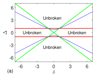
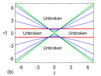
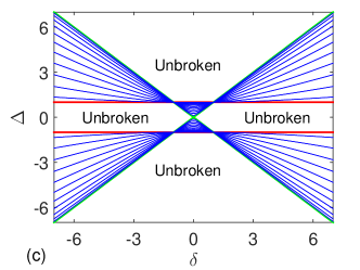
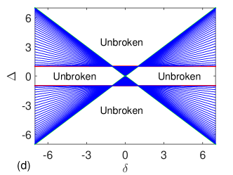
Figure 3: (Color online) Plots of the phase diagrams for the systems with $N=4,$ $8,$ $24$ and $66$, respectively. The phase boundary denoted by red $\left(k_{c}=0\right)$ and green lines separates the $\delta-\Delta$ plane into four regions. One can see that as $N$ increases, the ELs covers the area between the boundary lines. Note that the broken region does not include the origin, which corresponds to a degenerate point rather than an EP.

Before solving the Hamiltonian, we compare the Hamiltonian (13) and the Hamiltonian in Ref. HWH . We note that the existence of the real staggered potential $\lambda$ breaks the $\mathcal{PT}$ symmetry of the system and therefore leads to complex energies. The corresponding eigenstates do not possess any obvious symmetries except translation symmetry. It strongly implies that the anti-linear symmetry of the eigenstates is a key point in obtaining the full real spectrum. To obtain the spectrum and corresponding eigenstates, we take the Fourier transformation based on the translational symmetry,

$$A_{k}^{\dagger} = \frac{1}{\sqrt{N}}\sum_{j}e^{ikj}c_{2j-1}^{\dagger},$$ (14)

$$B_{k}^{\dagger} = \frac{1}{\sqrt{N}}\sum_{j}e^{ik\left(j+1/2\right)}c_{2j}^{\dagger},$$ (15)

satisfying

$$T^{-1}A_{k}^{\dagger}T=e^{-ik}A_{k}^{\dagger},\text{ }T^{-1}B_{k}^{\dagger}T=e^{-ik}B_{k}^{\dagger},$$ (16)

where $T$ is translational operator defined as $T^{-1}c_{j}^{\dagger}T=c_{j+2}^{\dagger}$. The commutation relation $\left[T,\mathcal{H}\right]=0$ ensures that the Hamiltonian can be diagonalized in invariant subspace spanned by the eigenvectors of operator $T$. Here $A_{k}$ and $B_{k}$ are annihilation operators of fermions with $k=2n\pi/N$ $\left(n\in\left[1,N\right]\right)$ at odd and even sites, respectively. Then the Hamiltonian (13) can be expressed as

$$\mathcal{H} = \frac{1}{2}\sum_{k}\left[\left(J_{0}\cos\frac{k}{2}-i\delta\sin\frac{k}{2}\right)A_{k}^{\dagger}B_{k}+\text{H.c.}\right]$$ (17)

$$+\left(i\Delta+\lambda\right)\sum_{k}\left(B_{k}^{\dagger}B_{k}-A_{k}^{\dagger}A_{k}\right)\text{,}$$

which is a bipartite lattice system consisting of two sub-lattices $A$ and $B$. By writing down the Hamiltonian (17) in the Nambu representation with the basis of $\left(A_{k}^{\dagger},B_{k}^{\dagger}\right)$, we have

$$\mathcal{H}=\sum_{k}\left(A_{k}^{\dagger},B_{k}^{\dagger}\right)\mathcal{H}_{k}\left(\begin{array}[]{c}A_{k}\\ B_{k}\end{array}\right),$$ (18)

where the core matrix is

$$\mathcal{H}_{k}=\left(\begin{array}[]{cc}-i\Delta-\lambda&J_{0}\cos\frac{k}{2}-i\delta\sin\frac{k}{2}\\ J_{0}\cos\frac{k}{2}+i\delta\sin\frac{k}{2}&i\Delta+\lambda\end{array}\right).$$ (19)

Note that $\mathcal{H}_{k}$ is similar to Eq. (1), which is critical to establish the classical correspondence of topological invariant. Based on the fact that $\left[\mathcal{H}_{k},\mathcal{H}_{k^{\prime}}\right]=0$, this Hamiltonian can be diagonalized via introducing canonical operators,

$$\alpha_{k} = u_{k}^{-}A_{k}+\nu_{k}^{-}B_{k},\text{ }\overline{\alpha}_{k}=u_{k}^{+}A_{k}^{\dagger}+\nu_{k}^{+}B_{k}^{\dagger},$$ (20)

$$\beta_{k} = \zeta_{k}^{-}A_{k}+\xi_{k}^{-}B_{k},\text{ }\overline{\beta}_{k}=\zeta_{k}^{+}A_{k}^{\dagger}+\xi_{k}^{+}B_{k}^{\dagger},$$ (21)

where the coefficients are

$$u_{k}^{\pm} = \frac{J_{0}\cos\left(k/2\right)\mp i\delta\sin\left(k/2\right)}{\sqrt{2\varepsilon_{k}\left(\varepsilon_{k}+i\Delta+\lambda\right)}},$$ (22)

$$\text{ }v_{k}^{\pm} = \frac{\varepsilon_{k}+i\Delta+\lambda}{\sqrt{2\varepsilon_{k}\left(\varepsilon_{k}+i\Delta+\lambda\right)}},$$ (23)

$$\zeta_{k}^{\pm} = \frac{J_{0}\cos\left(k/2\right)\mp i\delta\sin\left(k/2\right)}{\sqrt{2\varepsilon_{k}\left(\varepsilon_{k}-i\Delta-\lambda\right)}},$$ (24)

$$\text{ }\xi_{k}^{\pm} = \frac{-\varepsilon_{k}+i\Delta+\lambda}{\sqrt{2\varepsilon_{k}\left(\varepsilon_{k}-i\Delta-\lambda\right)}}.$$ (25)

Obviously, the complex modes $\left\{\alpha_{k},\overline{\alpha}_{k},\beta_{k},\overline{\beta}_{k}\right\}$ satisfy the canonical commutation relations

$$\left\{\overline{\alpha}_{k},\alpha_{k^{\prime}}\right\} = \left\{\overline{\beta}_{k},\beta_{k^{\prime}}\right\}=\delta_{kk^{\prime}},$$ (26)

$$\left\{\overline{\alpha}_{k},\overline{\alpha}_{k^{\prime}}\right\} = \left\{\overline{\beta}_{k},\overline{\beta}_{k^{\prime}}\right\}=0,$$ (27)

$$\left\{\overline{\alpha}_{k},\beta_{k^{\prime}}\right\} = \left\{\overline{\beta}_{k},\alpha_{k^{\prime}}\right\}=0,$$ (28)

$$\left\{\alpha_{k},\alpha_{k^{\prime}}\right\} = \left\{\beta_{k},\beta_{k^{\prime}}\right\}=0.$$ (29)

These relations enable the establishment of the biorthogonal bases thereby diagonalizing the Hamiltonian

$$\mathcal{H}=\sum_{k}\varepsilon_{k}\left(\overline{\alpha}_{k}\alpha_{k}-\overline{\beta}_{k}\beta_{k}\right),$$ (30)

here the single-particle spectrum in each subspace is

$$\varepsilon_{k}=\sqrt{J_{0}^{2}\cos^{2}\left(k/2\right)+\delta^{2}\sin^{2}\left(k/2\right)+\left(i\Delta+\lambda\right)^{2}}.$$ (31)

Note that the Hamiltonian $\mathcal{H}$ is still non-Hermitian owing to the fact that $\overline{\alpha}_{k}\left(\overline{\beta}_{k}\right)\neq\alpha_{k}^{\dagger}\left(\beta_{k}^{\dagger}\right)$. Accordingly, the eigenstates of $\mathcal{H}$ can be written in the form

$$\prod\limits_{\left\{k\right\}}\overline{\eta}_{k}\left|Vac\right\rangle,$$ (32)

where $\overline{\eta}_{k}$ represents either $\overline{\alpha}_{k}$ or $\overline{\beta}_{k}$. This constructs the biorthogonal set associated with the eigenstates

$$\left\langle Vac\right|\prod\limits_{\left\{k\right\}}\eta_{k}$$ (33)

of the Hamiltonian $\mathcal{H}^{{\dagger}}$, where $\left|Vac\right\rangle$ is the vacuum state of the fermion $c_{j}$. Next we move focus on the eigenstate $\left|GS\right\rangle$, which can be given as

$$\left|GS\right\rangle=\prod\limits_{k}\overline{\beta}_{k}\left|Vac\right\rangle,$$ (34)

and the corresponding birothogonal eigenstate of $\mathcal{H}^{{\dagger}}$ is

$$\left|\overline{GS}\right\rangle=\prod\limits_{k}\beta_{k}^{{\dagger}}\left|Vac\right\rangle.$$ (35)

The corresponding eigenenergy $-\sum_{k}\varepsilon_{k}$ is complex due to the existence of the complex on-site staggered potentials. As a reminder, these complex potentials also break the $\mathcal{PT}$ symmetry of the system. We would like to point out that the system can have full real spectrum in the absence of $\lambda$, which depends on whether the condition of $\left[J_{0}^{2}\cos^{2}\left(k/2\right)+\delta^{2}\sin^{2}\left(k/2\right)-\Delta^{2}\right]>0$ holds up. In the unbroken region, i.e, Im($\varepsilon_{k}$)$=0$, $\left|GS\right\rangle$ is the ground state of the system while the system possesses two gapped bands HWH . The alteration of the system parameters gives rise to the variation of the eigenstate symmetry. We are not concerned with whether the eigenstate $\left|GS\right\rangle$ is the ground state of the system. In this paper, we focus on the dynamical property of the $\left|GS\right\rangle$ in the following.

III.2 Phase diagram and EL

Now we turn to study the EPs of the system based on the previous solution. The EPs except the point $\left\{\Delta=\lambda=\delta=0,\text{ }k_{c}=\pi\right\}$, which corresponds to the degeneracy point rather than EP, can be identified via the condition $\varepsilon_{k}=0$. It is clear that when $\lambda=0$, any one of the momentum $k$ satisfies

$$J_{0}^{2}\cos^{2}\left(k/2\right)+\delta^{2}\sin^{2}\left(k/2\right)-\Delta^{2}=0,$$ (36)

admitting an exceptional curve in the $\delta-\Delta$ plane, at which the coefficients $u_{k}^{\pm}$, $v_{k}^{\pm}$, $\zeta_{k}^{\pm}$ and $\xi_{k}^{\pm}$ associated with corresponding canonical operators diverges. This feature is in agreement with that in the Ref. ZXZ . In addition, the eigenstate of the Nambu expression of $\mathcal{H}_{k}$ coalesces supporting another feature of EP. In Fig. 3, we plot the phase diagrams of the system. It shows that the ELs lie in the $\delta-\Delta$ plane. Each EL corresponds to two critical momentums $\pm k_{c}$, which is crucial to demonstrate the topological property of $\left|GS\right\rangle$.

It is worth pointing out that when $\Delta=0$, the system reduces to the Hermitian RM model. The two bands in this kind of systems with even sites touch each other at the point $\left\{\lambda=\delta=0,\text{ }k_{c}=\pi\right\}$. However, the EL can exist in the finite size of the system. In the thermodynamic limit $N\rightarrow\infty$, the phase boundary can be determined by the two straight lines corresponding to $k_{c}=0$, $\pi$, which is different from the dog-leg line in Ref. ZXZ . We plot these two lines in Fig. 3 with a red and a green lines, respectively. Moreover, in previous works TonyPRL , the topology of the EP can be characterized through the Zak phase which is associated with the bulk-boundary correspondence. The introducing of the Zak phase requires an infinite system with continuous $k$. This approach is not applicable to the study of finite non-Hermitian systems. In the following discussion, we remove this constraint and investigate the topology of the EP through the variation of the system parameters in the parameter space.

III.3 Topological invariant and classical correspondence

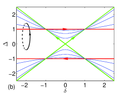
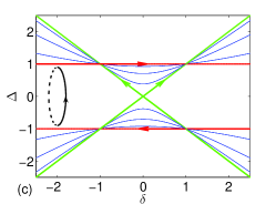
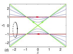
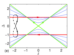
Figure 4: (Color online) Schematic illustration of different paths corresponding to the different values of Berry phases in the phase diagram with $N=8$. The black curve represents the closed evolution path and the other lines are the same as those in Fig. 3. The Berry phases are: (a) $0$, (b) $-\pi/2$, (c) $0$, (d) $\pi/2$, (e) $-\pi$, (f) $\pi$.

To demonstrate the topology of the system, according to the main conclusion in Sec. II, we assume that the Hamiltonian (13) is a periodic function of the system parameters $\left\{\lambda,\text{ }\Delta,\text{ }\delta\right\}$ that vary with time $t$, and $J_{0}$ is taken as a constant. The corresponding Berry connection $\overrightarrow{\mathcal{A}}=\left(\mathcal{A}_{\lambda},\text{ }\mathcal{A}_{\Delta},\text{ }\mathcal{A}_{\delta}\right)$ of the eigenstate $\left|GS\left(t\right)\right\rangle$ can be expressed as

$$\mathcal{A}_{g}=i\left\langle\overline{GS}\left(t\right)\right|\frac{\partial}{\partial g}\left|GS\left(t\right)\right\rangle,$$ (37)

where $\left|GS\left(t\right)\right\rangle$ represents the instantaneous eigenstate of the Hamiltonian $H\left(\lambda\left(t\right),\Delta\left(t\right),\delta\left(t\right)\right)$, and $g=\lambda$, $\Delta$, $\delta$ denote the three directions in the parameter space. The Berry connection can be explicitly expressed as

$$\overrightarrow{\mathcal{A}}=\sum_{k}\overrightarrow{\mathcal{A}}_{k},$$ (38)

where $\overrightarrow{\mathcal{A}}_{k}=\left(\mathcal{A}_{\lambda,k},\text{ }\mathcal{A}_{\delta,k},\text{ }\mathcal{A}_{\Delta,k}\right)$, and

$$\mathcal{A}_{g,k}=i\left\langle Vac\right|\beta_{k}\frac{\partial}{\partial g}\overline{\beta}_{k}\left|Vac\right\rangle$$ (39)

represents the Berry connection of the single-particle eigenstate. After some straightforward algebras, we have

$$\overrightarrow{\mathcal{A}}=\overrightarrow{\mathcal{A}}_{0}+\overrightarrow{\mathcal{A}}_{\pi},$$ (40)

where

$$\overrightarrow{\mathcal{A}}_{0} = \left(J_{0},\text{ }iJ_{0},\text{ }0\right)/\mathcal{D}_{0},$$ (41)

$$\overrightarrow{\mathcal{A}}_{\pi} = \left(\delta,\text{ }i\delta,\text{ }-\lambda-i\Delta\right)/\mathcal{D}_{\pi},$$ (42)

with $\mathcal{D}_{0}=2\varepsilon_{0}^{2}$ and $\mathcal{D}_{\pi}=2\varepsilon_{\pi}^{2}$. Here we can see that the Berry connection consists of two components, the contribution of which comes from the $k=0$, $\pi$, respectively. All the other $k$ contributes nothing to the total Berry connection owing to the fact that $\overrightarrow{\mathcal{A}}_{k}=-\overrightarrow{\mathcal{A}}_{2\pi-k}$. Note that we choose different gauges so that the single-particle eigenstates $\overline{\beta}_{0}\left|Vac\right\rangle$, $\overline{\beta}_{k}\left|Vac\right\rangle$ are smooth and single valued everywhere Xiao . According to the classical correspondence in Eq. (9), the boundary lines denoted by red and green color in Fig. 3 can act as four vortex filaments, the directions of which are sketched in Fig. 4. Therefore the Berry connection $\overrightarrow{\mathcal{A}}$ can be further expressed as

$$\overrightarrow{\mathcal{A}}_{0} = \overrightarrow{A}_{0}+i\nabla\varphi_{0},$$ (43)

$$\overrightarrow{\mathcal{A}}_{\pi} = \overrightarrow{A}_{\pi}+i\nabla\varphi_{\pi},$$ (44)

where

$$\overrightarrow{A}_{0}=\sum_{\sigma=\pm}\sigma\overrightarrow{A}_{0,\sigma},\text{ }\overrightarrow{A}_{\pi}=\sum_{\sigma=\pm}\sigma\overrightarrow{A}_{\pi,\sigma},$$ (45)

and the scalar potentials are

$$\varphi_{0} = \frac{1}{8}\ln\frac{D_{0,-}}{D_{0,+}},$$ (46)

$$\varphi_{\pi 0} = \frac{1}{8}\ln\frac{D_{\pi,-}}{D_{\pi,+}}.$$ (47)

with

$$D_{0,\pm} = \left(\Delta\pm J_{0}\right)^{2}+\lambda^{2},$$ (48)

$$D_{\pi,\pm} = \left(\Delta\pm\delta\right)^{2}+\lambda^{2}.$$ (49)

Moreover, the four curl fields with the form of

$$\overrightarrow{A}_{0,\pm} = \left(-\Delta\pm J_{0},\text{ }\lambda,\text{ }0\right)/4D_{0,\mp},$$ (50)

$$\overrightarrow{A}_{\pi,\pm} = \left(-\Delta\pm\delta,\text{ }\lambda,\text{ }\mp\lambda\right)/4D_{\pi,\mp},$$ (51)

are induced by vortex filaments of $\Delta=\pm J_{0}$, $\Delta=\pm\delta$ in $\Delta-\delta$ plane, respectively. In the context of classical electromagnetics, such the vortex filaments can be deemed as the magnetic field lines induced by solenoid. On the other hand, we consider the non-boundary ELs (blue hyperbolas in Fig. 3)that have nothing to do with the total Berry connection. It seems that each blue line is generated by the two hyperbolic solenoids with opposite current directions. However, the direct calculation shows that such a correspondence is incorrect. One cannot establish the connection between $\overrightarrow{\mathcal{A}}_{k}$ and $\overrightarrow{A}_{k}$ like Eqs. (43) and (44). In other words, the blue lines are not topological. This can also be understood in another way: For the momentum $k\neq 0$, $\pi$, the core matrix (19) can be decomposed into three Pauli operators as

$$\mathcal{H}_{k}=\overrightarrow{B}\cdot\overrightarrow{\sigma},$$ (52)

where $\overrightarrow{B}=\left(J_{0}\cos\frac{k}{2},\text{ }\delta\sin\frac{k}{2},\text{ }-\lambda-i\Delta\right)$. For the current form of field $\overrightarrow{B}$, a performance of a spin rotation reduces the system to containing two Pauli operators. However, such a spin rotation operator must be dependent on the system parameters $\left\{\lambda,\text{ }\Delta,\text{ }\delta\right\}$. This also indicates that there does not exist a parameter-independent chiral operator $C$ satisfying $\left\{C,\mathcal{H}_{k}\right\}=0$. Therefore, the main conclusion in Sec. II cannot be applied to the blue lines. In this point, not all the ELs can have classical correspondence.

Moreover, the corresponding Berry phase undergoing a closed path in the parameter space can be further expressed as $\gamma_{B}=\int_{C}\overrightarrow{\mathcal{A}}\cdot d\overrightarrow{l}=\int_{C}\overrightarrow{A}\cdot d\overrightarrow{l}$, which is identical to the magnetic flux penetrating the corresponding enclosed surface. In this point of view, the topology of the EL characterized by the Berry phase depends on the path of the closed curve. If the rotation direction of the curve judged by right handed screw rule is the same as the direction of red or green line, there is a $\pi/2$ contribution to Berry phase. Conversely, there is a $-\pi/2$ contribution to Berry phase. Furthermore, the blue lines does not contribute to the Berry phase because there are two opposing magnetic fluxes. As a result, the Berry phase is the sum of the contribution of red and green lines that penetrate the enclosed surface. We sketch several paths in Fig. 4, which corresponds to the different values of Berry phases (topological quantum numbers). Here are only a few simple examples in which the values of the Berry phase are taken between $-\pi$ and $\pi$. Through changing the form of the curve, the Berry phase can be any integer multiples of $\pi/2$. We would like to present here that the non-zero Berry curvature can be served as a dynamical signature to identify the existence of the EP in non-Hermitian systems.

For the finite system, the evolution path can pass through the region without ELs between red and green boundary lines. The topology of the EP can be characterized by the Berry phase in the parameter space rather than the Zak phase in the $k$ space of the infinite system. This provides an alternative way to describe the topology of the EP in finite non-Hermitian many-particle system. For the infinite system, the Berry phase is an integer multiples of $\pi$ since the existence of the EP lines prevent the selection of the closed path surrounding a single boundary line.

IV Summary and discussion

In summary, we have studied systematically the topology of the ELs in the parameter space through a simple non-Hermitian matrix. Based on the exact solution, the EL can be equivalent to a vortex filament in the classical physics. The curl field induced by the vortex filament is connected to the Berry connection of the non-Hermitian system through a gauge transformation. We apply this result to the core matrix of the non-Hermitian RM model and then find that the topological properties can be characterized by the Berry phase in the parameter space rather than Zak phase accumulated by an eigenstate during its parallel transport through the whole Brillouin zone. This findings provides an alternative way to investigate the topology of the EP in an experimentally accessible finite non-Hermitian lattice model with a discrete momentum space. Furthermore, based on the exact solution, we have shown that the boundary ELs associated with critical momenta $k_{c}=0$, $\pi$ can act as magnetic field lines induced by the infinite solenoids with infinitesimal diameter. For the non-boundary ELs, each line corresponds to two critical momenta $k_{c}$, $2\pi-k_{c}$ $\left(k_{c}\neq 0,\text{ }\pi\right)$, so all the non-boundary ELs make no contribution. Therefore, in this context, the Berry connection in the parameter space is equivalent to the vector potential generated by the four boundary ELs. From this perspective, the Berry phase is limited to an integer multiples of $\pi/2$, which is dependent on the magnetic flux of the area enclosed by trajectory. In addition, we would like to point that each boundary EL can have a direction, which can be determined by the corresponding Berry curvature. The non-zero Berry curvature can be deemed as a dynamical signature to identify the existence of the EP in the non-Hermitian systems.

- (1) M. V. Berry, Proc. R. Soc. A 392, 45 (1984).
- (2) D. Xiao, M.-C. Chang, and Q. Niu, Rev. Mod. Phys. 82, 1959 (2010).
- (3) J. C. Garrison and E. M. Wright, Phys. Lett. A 128, 177 (1988).
- (4) G. Dattoli, R.Mignani, and A. Torre, J. Phys. A 23, 5795 (1990).
- (5) C. Z. Ning and H. Haken, Phys. Rev. Lett. 68, 2109 (1992).
- (6) D. J. Moore and G. E. Stedman, Phys. Rev. A 45, 513 (1992).
- (7) X. C. Gao, J. B. Xu, and T. Z. Qian, Phys. Rev. A 46, 3626 (1992).
- (8) Marcel Pont, R. M. Potvliege, Robin Shakeshaft, and Philip H. G. Smith, Phys. Rev. A 46, 555 (1992).
- (9) S. Massar, Phys. Rev. A 54, 4770 (1996).
- (10) Y. C. Ge and M. S. Child, Phys. Rev. A 58, 872 (1998).
- (11) R. S. Whitney, Y. Makhlin, A. Shnirman, and Y. Gefen, Phys. Rev. Lett. 94, 070407 (2005).
- (12) H. Mehri-Dehnavi and A. Mostafazadeh, J. Math. Phys. 49, 082105 (2008).
- (13) A. I. Nesterov and S. G. Ovchinnikov, Phys. Rev. E 78, 015202(R) (2008).
- (14) X. D. Cui and Y. J. Zheng, Phys. Rev. A 86, 064104 (2012).
- (15) S. D. Liang and G. Y. Huang, Phys. Rev. A 87, 012118 (2013).
- (16) X. Z. Zhang, and Z. Song, Phys. Rev. A, 88, 042108 (2013).
- (17) D. J. Thouless, M. Kohmoto, M. P. Nightingale, and M. den Nijs, Phys. Rev. Lett. 49, 405 (1982).
- (18) C. L. Kane and E. J. Mele, Phys. Rev. Lett. 95, 226801 (2005).
- (19) J. E. Moore and L. Balents, Phys. Rev. B 75, 121306 (2007).
- (20) L. Fu, C. L. Kane, and E. J. Mele, Phys. Rev. Lett. 98, 106803 (2007).
- (21) L. Fu and C. L. Kane, Phys. Rev. B 76, 045302 (2007).
- (22) A. P. Schnyder, S. Ryu, A. Furusaki, and A. W. W. Ludwig, Phys. Rev. B 78, 195125 (2008).
- (23) A. Kitaev, in AIP Conf. Proc., Vol. 22 (AIP, 2009) pp. 22-30, arXiv: 0901.2686.
- (24) A. Bansil, H. Lin, and T. Das, Rev. Mod. Phys. 88, 021004 (2016).
- (25) C.-K. Chiu, J. C. Y. Teo, A. P. Schnyder, and S. Ryu, Rev. Mod. Phys. 88, 035005 (2016).
- (26) N. P. Armitage, E. J. Mele, and A. Vishwanath, arXiv: 1705.01111 (2017).
- (27) J. Zak, Phys. Rev. Lett. 62, 2747 (1989).
- (28) R. Resta, Rev. Mod. Phys. 66, 899 (1994).
- (29) N. Moiseyev, Non-Hermitian Quantum Mechanics (Cambridge University Press, Cambridge, England, 2011).
- (30) Y. C. Hu and T. L. Hughes, Phys. Rev. B 84, 153101 (2011), arXiv:1107.1064.
- (31) K. Esaki, M. Sato, K. Hasebe, and M. Kohmoto, Phys. Rev. B 84, 205128 (2011).
- (32) T. E. Lee, Phys. Rev. Lett., 116, 133903 (2016).
- (33) D. Leykam, K. Y. Bliokh, C. Huang, Y. D. Chong, and F. Nori, Phys. Rev. Lett. 118, 040401 (2017).
- (34) Y. Xu, S.-T. Wang, and L.-M. Duan, Phys. Rev. Lett. 118, 045701 (2017).
- (35) W. Hu, H. Wang, P. P. Shum, and Y. D. Chong, Phys. Rev. B 95, 184306 (2017).
- (36) Y. Xiong, arXiv: 1705.06039 (2017).
- (37) R. Uzdin, A. Mailybaev, and N. Moiseyev, J. Phys. A Math. Theor. 44, 435302 (2011).
- (38) M. V. Berry and R. Uzdin, J. Phys. A Math. Theor. 44, 435303 (2011).
- (39) M. V. Berry, J. Opt. 13, 115701 (2011).
- (40) I. Gilary, A. A. Mailybaev, and N. Moiseyev, Phys. Rev. A 88, 010102 (2013).
- (41) E.-M. Graefe, A. A. Mailybaev, and N. Moiseyev, Phys. Rev. A 88, 033842 (2013).
- (42) P. R. Kaprálová-Zánská and N. Moiseyev, J. Chem. Phys. 141, 014307 (2014).
- (43) T. J. Milburn, J. Doppler, C. A. Holmes, S. Portolan, S. Rotter, and P. Rabl, Phys. Rev. A 92, 052124 (2015).
- (44) J. Doppler, A. A. Mailybaev, J. Böhm, U. Kuhl, A. Girschik, F. Libisch, T. J. Milburn, P. Rabl, N. Moiseyev, and S. Rotter, Nature 537, 76 (2016).
- (45) H. Xu, D. Mason, L. Jiang, and J. G. E. Harris, Nature 537, 80 (2016).
- (46) J. K. Chin et al., Nature (London) 443, 961 (2006).
- (47) N. Strohmaier, Phys. Rev. Lett. 99, 220601 (2007).
- (48) L. Hacke, Science, 327, 1621 (2010).
- (49) S. Longhi, Phys. Rev. A, 88, 052102 (2013).
- (50) W. H. Hu, L. Jin, Y. Li, and Z. Song, Phys. Rev. A, 86, 042110 (2012).
- (51) S. Lin, X. Z. Zhang, and Z. Song, Phys. Rev. A, 92, 012117 (2015).