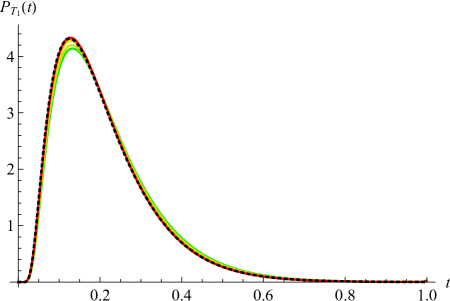
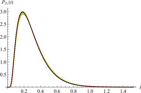
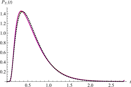
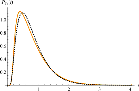
First passage in an interval for fractional Brownian motion

Kay Jörg Wiese CNRS-Laboratoire de Physique Théorique de l’Ecole Normale Supérieure, 24 rue Lhomond, 75005 Paris, France, PSL University, Sorbonne Université.
Abstract

Be Xtsubscript𝑋𝑡X_{t} a random process starting at x[0,1]𝑥01x\in[0,1] with absorbing boundary conditions at both ends of the interval. Denote P1(x)subscript𝑃1𝑥P_{1}(x) the probability to first exit at the upper boundary. For Brownian motion, P1(x)=xsubscript𝑃1𝑥𝑥P_{1}(x)=x, equivalent to P1(x)=1superscriptsubscript𝑃1𝑥1P_{1}^{\prime}(x)=1. For fractional Brownian motion with Hurst exponent H𝐻H, we establish that P1(x)=𝒩[x(1x)]1H2eϵ(x)+𝒪(ϵ2)superscriptsubscript𝑃1𝑥𝒩superscriptdelimited-[]𝑥1𝑥1𝐻2superscript𝑒italic-ϵ𝑥𝒪superscriptitalic-ϵ2P_{1}^{\prime}(x)={\cal N}[x(1-x)]^{\frac{1}{H}-2}e^{\epsilon{\cal F}(x)+{\cal O}(\epsilon^{2})}, where ϵ=H12italic-ϵ𝐻12\epsilon=H-\frac{1}{2}. The function (x)𝑥{\cal F}(x) is analytic, and well approximated by its Taylor expansion, (x)16(C1)(x1/2)2+𝒪(x1/2)4similar-to-or-equals𝑥16𝐶1superscript𝑥122𝒪superscript𝑥124{\cal F}(x)\simeq 16(C-1)(x-1/2)^{2}+{\cal O}(x-1/2)^{4}, where C=0.915𝐶0.915C=0.915... is the Catalan-constant. A similar result holds for moments of the exit time starting at x𝑥x. We then consider the span of Xtsubscript𝑋𝑡X_{t}, i.e. the size of the (compact) domain visited up to time t𝑡t. For Brownian motion, we derive an analytic expression for the probability that the span reaches 1 for the first time, then generalized to fBm. Using large-scale numerical simulations with system sizes up to N=224𝑁superscript224N=2^{24} and a broad range of H𝐻H, we confirm our analytic results. There are important finite-discretization corrections which we quantify. They are most severe for small H𝐻H, necessitating to go to the large systems mentioned above.

I Introduction

A key problem in stochastic processes are the first-passage properties FellerBook ; RednerBook in a finite domain, say the unit interval [0,1]01[0,1]. For Brownian motion, the probability to exit at the upper boundary x=1𝑥1x=1, starting at x𝑥x is

P10(x)=x.subscriptsuperscript𝑃01𝑥𝑥P^{0}_{1}(x)=x\ . (1)

Another key observable is the exit time, starting at x𝑥x, which behaves as Texit(x)0x(1x)similar-tosubscriptdelimited-⟨⟩subscript𝑇exit𝑥0𝑥1𝑥\left<T_{\rm exit}(x)\right>_{0}\sim x(1-x). Many physical situations, however, cannot be described by Brownian motion. An example is a polymer translocating through a nano-pore. While the motion of the polymer as a whole is a Markov process, the effective process for its position in the pore is non-Markovian Muthukumar1999 ; LubenskyNelson1999 ; StormStormChenZandbergenJoannyDekker2005 ; PanjaBarkema2010 ; PanjaBarkemaBall2007 ; ZoiaRossoMajumdar2009 .
Refer to caption
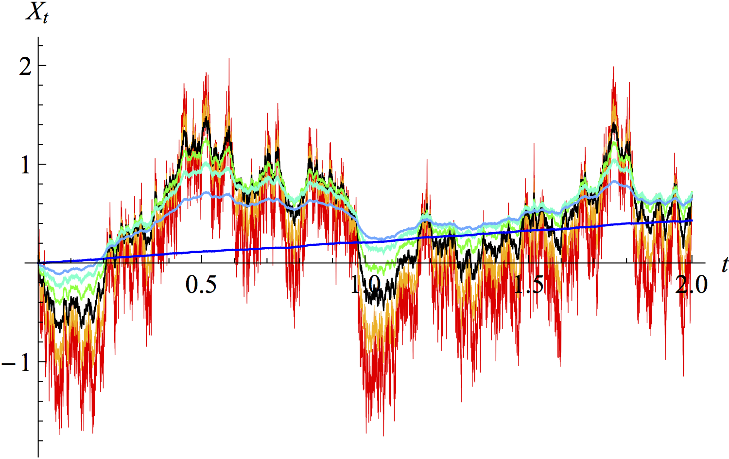
Figure 1: Realizations of a fBm for H=0.25𝐻0.25H=0.25 (red, roughest curve), H=0.375𝐻0.375H=0.375 (orange), H=1/2𝐻12H=1/2, Brownian (black), H=0.625𝐻0.625H=0.625 (green), H=0.75𝐻0.75H=0.75 (cyan), H=0.875𝐻0.875H=0.875 (bright blue) to H=1𝐻1H=1 (dark blue, straight line), using the algorithm of Davies and Harte DaviesHarte1987 ; DiekerPhD ; DiekerMandjes2003 .

The questions posed above become much more involved for the latter. The simplest generalization is fractional Brownian motion (fBm): It is the unique process that retains from Brownian motion Gaussianity, scale and translational invariance both in space and time, and that is drift-free. FBm was introduced in its final form by Mandelbrot and Van Ness MandelbrotVanNess1968 . It is indexed by the Hurst exponent H𝐻H, with 0<H10𝐻10<H\leq 1 (see Fig. 1). As Gaussian process, it is specified by its second moment,

X(t1)X(t2)=t12H+t22H|t1t2|2H.delimited-⟨⟩𝑋subscript𝑡1𝑋subscript𝑡2superscriptsubscript𝑡12𝐻superscriptsubscript𝑡22𝐻superscriptsubscript𝑡1subscript𝑡22𝐻\left<X(t_{1})X(t_{2})\right>=t_{1}^{2H}+t_{2}^{2H}-|t_{1}-t_{2}|^{2H}\ . (2)

FBm is important as it successfully models a variety of natural processes DecreusefondUstunel1998 ; MetzlerKlafter2000 : a tagged particle in single-file diffusion (H= 0.25𝐻0.25H\,{=}\,0.25) (KrapivskyMallickSadhu2015, ; SadhuDerrida2015, ), the integrated current in diffusive transport (H= 0.25𝐻0.25H\,{=}\,0.25) SadhuDerrida2016 , polymer translocation through a narrow pore (H 0.4similar-to-or-equals𝐻0.4H\,{\simeq}\,0.4) ZoiaRossoMajumdar2009 ; DubbeldamRostiashvili2011 ; PalyulinAlaNissilaMetzler2014 , anomalous diffusion BouchaudGeorges1990 , values of the log return of a stock (H 0.6to 0.8similar-to-or-equals𝐻0.6to0.8H\,{\simeq}\,0.6\;{\rm to}\;0.8) CutlandKoppWillinger1995 ; Sottinen2001 , hydrology (H 0.72to 0.87similar-to-or-equals𝐻0.72to0.87H\,{\simeq}\,0.72\;{\rm to}\;0.87) MandelbrotWallis1968 , a tagged monomer in a polymer (H= 0.25𝐻0.25H\,{=}\,0.25) GuptaRossoTexier2013 , solar flare activity (H 0.57to 0.86similar-to-or-equals𝐻0.57to0.86H\,{\simeq}\,0.57\;{\rm to}\;0.86) Monte-MorenoHernandez-Pajares2014 , the price of electricity in a liberated market (H 0.41similar-to-or-equals𝐻0.41H\,{\simeq}\,0.41) Simonsen2003 , telecommunication networks (H 0.78to 0.86similar-to-or-equals𝐻0.78to0.86H\,{\simeq}\,0.78\;{\rm to}\;0.86) Norros1995 , telomeres inside the nucleus of human cells (H 0.18to 0.35similar-to-or-equals𝐻0.18to0.35H\,{\simeq}\,0.18\;{\rm to}\;0.35) BurneckiKeptenJanczuraBronshteinGariniWeron2012 , or diffusion inside crowded fluids (H 0.4similar-to-or-equals𝐻0.4H\,{\simeq}\,0.4) ErnstHellmannKohlerWeiss2012 .

There are yet no analytical methods to treat the questions posed above for H𝐻H other than 1/2121/2 (Brownian motion) and H=1𝐻1H=1 (a straight line with a random slope). To remedy this, we developed tools WieseMajumdarRosso2010 ; DelormeWiese2015 ; DelormeRossoWiese2017 ; DelormeWiese2016b ; DelormeWiese2016 ; DelormeThesis which allow us to answer this question analytically, in a Taylor expansion around H=1/2𝐻12H=1/2, i.e. in

ϵ=H12.italic-ϵ𝐻12\epsilon=H-\frac{1}{2}\ . (3)

These methods have proven feasible and precise up to second order in ϵitalic-ϵ\epsilon SadhuDelormeWiese2017 , where they allowed us to distinguish the three classical arcsine laws.
Refer to caption
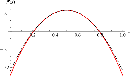
Figure 2: The scaling function (x)𝑥{\cal F}(x) defined in Eq. (72) (solid, red), normalized s.t. that 01(x)dx=0superscriptsubscript01𝑥differential-d𝑥0\int_{0}^{1}{\cal F}(x)\,\mathrm{d}x=0. The dashed line is the quadratic term given in Eq. (8).

In this article, we generalize the exit probability and distribution of exit times to fractional Brownian motion (Fig. 1). It had earlier been argued MajumdarRossoZoia2010b that the exit probability at the upper boundary scales for small x𝑥x as

P1(x)xϕ,ϕ=θH,formulae-sequencesimilar-tosubscript𝑃1𝑥superscript𝑥italic-ϕitalic-ϕ𝜃𝐻P_{1}(x)\sim x^{\phi}\ ,\qquad\phi=\frac{\theta}{H}\ , (4)

and where θ𝜃\theta is the persistence exponent. For fBm Majumdar1999 ; WieseMajumdarRosso2010

θ=1H.𝜃1𝐻\theta=1-H\ . (5)

This led the authors of Ref. MajumdarRossoZoia2010b to conjecture that P1(x)[x(1x)]1H2similar-tosuperscriptsubscript𝑃1𝑥superscriptdelimited-[]𝑥1𝑥1𝐻2P_{1}^{\prime}(x)\sim[x(1-x)]^{\frac{1}{H}-2}, for all x𝑥x. This however is too simple an approximation MajumdarRossoZoia2010b .
Refer to caption
Refer to caption
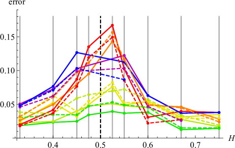
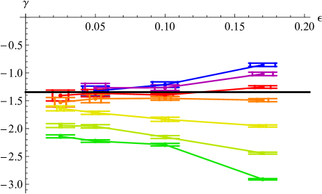
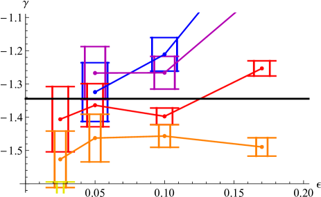
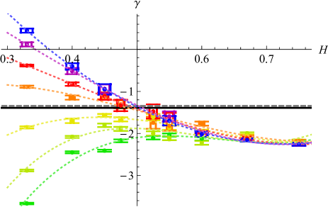
Figure 3: The effective measured curvature γ𝛾\gamma, as function of H𝐻H, and system size. The grey dashed line is γ𝛾\gamma as given by Eq. (118); the black solid line at 1.391.39-1.39 is a fit to the curvature of (x)𝑥{\cal F}(x) in the range 0.150.150.15 to 0.850.850.85. The color code is (from bottom to top on the left plot) N=213𝑁superscript213N=2^{13} (dark green), 214superscript2142^{14} (green), 216superscript2162^{16} (olive), 218superscript2182^{18} (orange), 220superscript2202^{20} (red), 222superscript2222^{22} (dark magenta), 224superscript2242^{24} (blue). The 1-σ𝜎\sigma errors are indicated with bars on the left, and are explicitly shown on the right. There the solid lines are the measured errors obtained as follows: γ𝛾\gamma is estimated by fitting a parabola to each of the data sets presented on Fig. 13, and measuring the variance of the data minus the fit, which allows to estimate the error of the fit, after calibration on white noise. The dashed lines are proportional to the square root of the number of samples, divided by |ϵ|italic-ϵ|\epsilon|, and calibrated against the estimated data to have a second independent estimate. The grey lines are a guide to the eye, at the location of the H𝐻H-values considered, H=0.33𝐻0.33H=0.33, 0.40.40.4, 0.450.450.45, 0.4750.4750.475, 0.5250.5250.525, 0.550.550.55, 0.60.60.6, 0.670.670.67, 0.750.750.75.

Here we show analytically that P1(x)superscriptsubscript𝑃1𝑥P_{1}^{\prime}(x) can be written in the form

P1(x)subscriptsuperscript𝑃1𝑥\displaystyle P^{\prime}_{1}(x) =\displaystyle= 𝒩[x(1x)]1H2eϵ(x)+𝒪(ϵ2),𝒩superscriptdelimited-[]𝑥1𝑥1𝐻2superscript𝑒italic-ϵ𝑥𝒪superscriptitalic-ϵ2\displaystyle{\cal N}[x(1-x)]^{\frac{1}{H}-2}e^{\epsilon{\cal F}(x)+{\cal O}(\epsilon^{2})}\ , (6)

where (x)𝑥{\cal F}(x) is an analytic function,

(x)𝑥\displaystyle{\cal F}(x) =\displaystyle= 4[12ζ(1)+ln(2)3+ln(x(1x))\displaystyle 4\bigg{[}12\zeta^{\prime}(-1)+\frac{\ln(2)}{3}+\ln\!\big{(}x(1-x)\big{)} (7)
+ln(Γ(12x2))ln(Γ(1x2))Γ12𝑥2Γ1𝑥2\displaystyle~{}~{}~{}+\ln\!\bigg{(}\!\Gamma\!\Big{(}{\frac{1}{2}-\frac{x}{2}}\Big{)}\!\bigg{)}-\ln\!\bigg{(}\!\Gamma\!\Big{(}1-\frac{x}{2}\Big{)}\!\bigg{)}
+ln(Γ(x2))ln(Γ(x+12))].\displaystyle~{}~{}~{}+\ln\!\bigg{(}\!\Gamma\!\Big{(}\frac{x}{2}\Big{)}\!\bigg{)}-\ln\!\bigg{(}\!\Gamma\!\Big{(}\frac{x+1}{2}\Big{)}\!\bigg{)}\bigg{]}\ .

Absorbing the constant into the normalization 𝒩𝒩\cal N, its Taylor-expansion reads

(x)𝑥\displaystyle{\cal F}(x) =\displaystyle= 4203ln(2)+8[ln(Γ(14))ln(Γ(34))+6ζ(1)]420328delimited-[]Γ14Γ346superscript𝜁1\displaystyle\textstyle 4-\frac{20}{3}\ln(2)+8\big{[}\ln\!\big{(}\Gamma(\frac{1}{4})\big{)}-\ln\!\big{(}\Gamma(\frac{3}{4})\big{)}+6\zeta^{\prime}(-1)\big{]} (8)
+16(C1)(x12)216𝐶1superscript𝑥122\displaystyle+16(C-1)(x-{\textstyle\frac{1}{2}})^{2}
+148(x12)4[ψ(3)(14)ψ(3)(34)1536]148superscript𝑥124delimited-[]superscript𝜓314superscript𝜓3341536\displaystyle\textstyle+\frac{1}{48}(x-{\textstyle\frac{1}{2}})^{4}\left[\psi^{(3)}({\textstyle\frac{1}{4}})-\psi^{(3)}({\textstyle\frac{3}{4}})-1536\right]
+𝒪(x12)6𝒪superscript𝑥126\displaystyle+{\cal O}({\textstyle x-\frac{1}{2}})^{6}
=\displaystyle= 0.1167361.34455(x12)20.353774(x12)40.1167361.34455superscript𝑥1220.353774superscript𝑥124\displaystyle 0.116736-1.34455(x-{\textstyle\frac{1}{2}})^{2}-0.353774(x-{\textstyle\frac{1}{2}})^{4}
+𝒪(x12)6.𝒪superscript𝑥126\displaystyle+{\cal O}({\textstyle x-\frac{1}{2}})^{6}\ .

The number C𝐶C is the Catalan constant

C=n=0(1)n(2n+1)20.915965594𝐶superscriptsubscript𝑛0superscript1𝑛superscript2𝑛120.915965594C=\sum_{n=0}^{\infty}\frac{(-1)^{n}}{(2n+1)^{2}}\approx 0.915965594... (9)

and ψ(3)(x)=x4ln(Γ(x))superscript𝜓3𝑥superscriptsubscript𝑥4Γ𝑥\psi^{(3)}(x)=\partial_{x}^{4}\ln(\Gamma(x)) the polygamma function of order 3. As can be seen on Fig. 2, the function (x)𝑥{\cal F}(x) is well approximated by its second Taylor-coefficient. Incorporating the forth order term, analytic result and Taylor expansion are indistinguishable on this plot. As a consequence, the most relevant information is captured by the curvature of (x)𝑥{\cal F}(x) at x=1/2𝑥12x=1/2,

γ:=12′′(x)|x=1/2=16(C1).assign𝛾evaluated-at12superscript′′𝑥𝑥1216𝐶1\gamma:=\frac{1}{2}{\cal F}^{\prime\prime}(x)\Big{|}_{x=1/2}=16(C-1)\ . (10)

We believe that higher-order terms in ϵitalic-ϵ\epsilon entering into the exponential of Eq. (6) are also analytic, and well approximated by their low-order (in x𝑥x) Taylor coefficients. We can therefore ask how the effective curvature γ𝛾\gamma, defined by the first equality in Eq. (10), changes with H𝐻H. The answer can be read off from Fig. 3: Consider the top (blue) data on the left plot, obtained for the largest systems. One sees that γ𝛾\gamma depends on H𝐻H, and that for H12𝐻12H\to\frac{1}{2} it extrapolates to γ=1.34±0.02𝛾plus-or-minus1.340.02\gamma=-1.34\pm 0.02, in agreement with the analytical result (8).

This article is organized as follows: We first derive key results for Brownian motion, see section II. Most of them are known FellerBook ; RednerBook , except for the span-observables. After a short review of the ϵitalic-ϵ\epsilon-expansion in section III, we derive in section IV the leading-order corrections for fBm for a number of key observables. All our results are checked via extensive numerical simulations in section V. We conclude in section VI.

II Basic formulas for Brownian Motion with two absorbing boundaries

II.1 Solving the Fokker-Planck equation

Brownian motion from x𝑥x to y𝑦y in time t𝑡t satisfies the forward Fokker-Planck equation FellerBook ; RednerBook

tP+(x,y,t)=y2P+(x,y,t)subscript𝑡subscript𝑃𝑥𝑦𝑡superscriptsubscript𝑦2subscript𝑃𝑥𝑦𝑡\partial_{t}P_{+}(x,y,t)=\partial_{y}^{2}P_{+}(x,y,t) (11)

The plus refers to surviving paths. Its general solution with absorbing walls at x=0𝑥0x=0 and x=1𝑥1x=1 can be written as

P+(x,y,t)subscript𝑃𝑥𝑦𝑡\displaystyle P_{+}(x,y,t) (12)
=\displaystyle= 14πtn=(e(xy+2n)2/4te(x+y+2n)2/4t)14𝜋𝑡superscriptsubscript𝑛superscript𝑒superscript𝑥𝑦2𝑛24𝑡superscript𝑒superscript𝑥𝑦2𝑛24𝑡\displaystyle\frac{1}{\sqrt{4\pi t}}\sum_{n=-\infty}^{\infty}\left(e^{-(x-y+2n)^{2}/4t}-e^{-(x+y+2n)^{2}/4t}\right)
=\displaystyle= 12ϑ3(π2(xy),eπ2t)12ϑ3(π2(x+y),eπ2t).12subscriptitalic-ϑ3𝜋2𝑥𝑦superscript𝑒superscript𝜋2𝑡12subscriptitalic-ϑ3𝜋2𝑥𝑦superscript𝑒superscript𝜋2𝑡\displaystyle\frac{1}{2}\vartheta_{3}\!\left(\frac{\pi}{2}(x-y),e^{-\pi^{2}t}\right)-\frac{1}{2}\vartheta_{3}\!\left(\frac{\pi}{2}(x+y),e^{-\pi^{2}t}\right).~{}~{}~{}~{}~{}~{}~{}~{}

ϑitalic-ϑ\vartheta is the elliptic ϑitalic-ϑ\vartheta-function. To prove this statement it is enough to remark that the first line satisfies the Fokker-Planck equation (11), vanishes at y=0𝑦0y=0 and y=1𝑦1y=1, and reduces for t0𝑡0t\to 0 to a δ𝛿\delta-function

limt0P+(x,y,t)=δ(xy).subscript𝑡0subscript𝑃𝑥𝑦𝑡𝛿𝑥𝑦\lim_{t\to 0}P_{+}(x,y,t)=\delta(x-y)\ . (13)

Let us introduce the notation

(z,t):=14πtn=e(z+2n)2/4t=12ϑ3(π2z,eπ2t).assign𝑧𝑡14𝜋𝑡superscriptsubscript𝑛superscript𝑒superscript𝑧2𝑛24𝑡12subscriptitalic-ϑ3𝜋2𝑧superscript𝑒superscript𝜋2𝑡{\mathbb{P}}(z,t):=\frac{1}{\sqrt{4\pi t}}\sum_{n=-\infty}^{\infty}e^{-(z+2n)^{2}/4t}=\frac{1}{2}\vartheta_{3}\!\left(\frac{\pi}{2}z,e^{-\pi^{2}t}\right). (14)

In terms of this function, Eq. (12) can be written as

P+(x,y,t)=(xy,t)(x+y,t).subscript𝑃𝑥𝑦𝑡𝑥𝑦𝑡𝑥𝑦𝑡{P_{+}(x,y,t)}={\mathbb{P}}(x-y,t)-{\mathbb{P}}(x+y,t)\ . (15)

Using the Poisson summation formula, an alternative form for (z,t)𝑧𝑡{\mathbb{P}}(z,t) is

(z,t)=12+m=1em2π2tcos(mπz).𝑧𝑡12superscriptsubscript𝑚1superscript𝑒superscript𝑚2superscript𝜋2𝑡𝑚𝜋𝑧{\mathbb{P}}(z,t)=\frac{1}{2}+\sum_{m=1}^{\infty}e^{-m^{2}\pi^{2}t}\cos(m\pi z)\ . (16)

It is useful to consider its Laplace-transformed version. We define the Laplace transform of a function F(t)𝐹𝑡F(t), with t0𝑡0t\geq 0, and marked with a tilde as

F~(s):=0dtestF(t).assign~𝐹𝑠superscriptsubscript0differential-d𝑡superscript𝑒𝑠𝑡𝐹𝑡\tilde{F}(s):=\int_{0}^{\infty}\mathrm{d}t\,e^{-st}F(t)\ . (17)

This yields

P~+(x,y,s)subscript~𝑃𝑥𝑦𝑠\displaystyle\!\!\!\tilde{P}_{+}(x,y,s) =\displaystyle= es|xy|es(x+y)2ssuperscript𝑒𝑠𝑥𝑦superscript𝑒𝑠𝑥𝑦2𝑠\displaystyle\frac{e^{-\sqrt{s}|x-y|}-e^{-\sqrt{s}(x+y)}}{2\sqrt{s}} (18)
[coth(s)1]sinh(sx)sinh(sy)s.delimited-[]hyperbolic-cotangent𝑠1𝑠𝑥𝑠𝑦𝑠\displaystyle-\frac{\left[\coth(\sqrt{s})-1\right]\sinh(\sqrt{s}x)\sinh(\sqrt{s}y)}{\sqrt{s}}.~{}~{}~{}~{}~{}~{}~{}

According to Eq. (15) a form which only depends on xy𝑥𝑦x-y and x+y𝑥𝑦x+y also exists. We use the form (18), since the factorization of the second term facilitates its integration.

II.2 Boundary currents and conservation of probability

Conservation of probability reads (the variable x𝑥x is the initial condition, here a dummy variable)

tP+(x,y,t)+yJ(x,y,t)=0.subscript𝑡subscript𝑃𝑥𝑦𝑡subscript𝑦𝐽𝑥𝑦𝑡0\partial_{t}P_{+}(x,y,t)+\partial_{y}J(x,y,t)=0\ . (19)

J𝐽J is the current, which from Eq. (19) can be identified as

J(x,y,t)=yP+(x,y,t).𝐽𝑥𝑦𝑡subscript𝑦subscript𝑃𝑥𝑦𝑡J(x,y,t)=-\partial_{y}P_{+}(x,y,t)\ . (20)

Due to the Dirichlet conditions at y=0𝑦0y=0 and y=1𝑦1y=1, we have

01dytP+(x,y,t)=J(x,0,t)J(x,1,t).superscriptsubscript01differential-d𝑦subscript𝑡subscript𝑃𝑥𝑦𝑡𝐽𝑥0𝑡𝐽𝑥1𝑡\int_{0}^{1}\mathrm{d}y\,\partial_{t}P_{+}(x,y,t)=J(x,0,t)-J(x,1,t)\ . (21)

We find

J(x,y,t)𝐽𝑥𝑦𝑡\displaystyle J(x,y,t) =\displaystyle= π4ϑ3(π2(xy),eπ2t)𝜋4superscriptsubscriptitalic-ϑ3𝜋2𝑥𝑦superscript𝑒superscript𝜋2𝑡\displaystyle\frac{\pi}{4}\vartheta_{3}^{\prime}\!\left(\frac{\pi}{2}(x-y),e^{-\pi^{2}t}\right) (22)
+π4ϑ3(π2(x+y),eπ2t).𝜋4superscriptsubscriptitalic-ϑ3𝜋2𝑥𝑦superscript𝑒superscript𝜋2𝑡\displaystyle+\frac{\pi}{4}\vartheta_{3}^{\prime}\!\left(\frac{\pi}{2}(x+y),e^{-\pi^{2}t}\right)\ .

The derivatives of the elliptic ϑitalic-ϑ\vartheta functions are w.r.t. its first argument. The probability to exit at time t𝑡t, when starting at x𝑥x for time 00 reads

Pexit(x,t)subscript𝑃exit𝑥𝑡\displaystyle P_{\rm exit}(x,t) =\displaystyle= Jtot(x,t)=J(x,1,t)J(x,0,t)subscript𝐽tot𝑥𝑡𝐽𝑥1𝑡𝐽𝑥0𝑡\displaystyle-J_{\rm tot}(x,t)=J(x,1,t)-J(x,0,t)
=\displaystyle= π2[ϑ3(π2(x1),eπ2t)ϑ3(πx2,eπ2t)].𝜋2delimited-[]superscriptsubscriptitalic-ϑ3𝜋2𝑥1superscript𝑒superscript𝜋2𝑡superscriptsubscriptitalic-ϑ3𝜋𝑥2superscript𝑒superscript𝜋2𝑡\displaystyle\frac{\pi}{2}\left[\vartheta_{3}^{\prime}\!\left(\frac{\pi}{2}(x-1),e^{-\pi^{2}t}\right)-\vartheta_{3}^{\prime}\!\left(\frac{\pi x}{2},e^{-\pi^{2}t}\right)\right].

Going to Laplace variables, we find

1+s01dyP~(x,y,s)=J~(x,0,s)J~(x,1,s).1𝑠superscriptsubscript01differential-d𝑦~𝑃𝑥𝑦𝑠~𝐽𝑥0𝑠~𝐽𝑥1𝑠-1+s\int_{0}^{1}\mathrm{d}y\,\tilde{P}(x,y,s)=\tilde{J}(x,0,s)-\tilde{J}(x,1,s)\ . (24)

The outgoing currents of the Laplace transform are

J~(x,0,s)~𝐽𝑥0𝑠\displaystyle-\tilde{J}(x,0,s) =\displaystyle= sinh(s(1x))sinh(s),𝑠1𝑥𝑠\displaystyle\frac{\sinh\big{(}\sqrt{s}(1-x)\big{)}}{\sinh(\sqrt{s})}\ , (25)
J~(x,1,s)~𝐽𝑥1𝑠\displaystyle\tilde{J}(x,1,s) =\displaystyle= sinh(sx)sinh(s).𝑠𝑥𝑠\displaystyle\frac{\sinh(\sqrt{s}\,x)}{\sinh(\sqrt{s})}\ . (26)
Refer to caption
Refer to caption
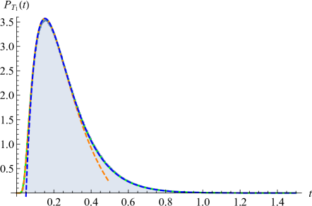
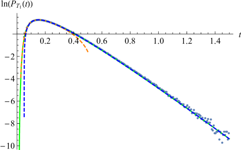
Figure 4: The probability that the span reaches 1 for the first time. Grey: RW simulation with δt=105𝛿𝑡superscript105\delta t=10^{-5}, and 106superscript10610^{6} samples. Green: the analytic result (39). Orange dashed the small-times asymptote (41); blue dashed the large-time asymptote (42). Note a small systematic deviation due to the relatively large time step δt=105𝛿𝑡superscript105\delta t=10^{-5}.

II.3 Absorption probabilities at x=0𝑥0x=0 and x=1𝑥1x=1

The absorption probabilities at x=0𝑥0x=0 and x=1𝑥1x=1 are

P0(x)subscript𝑃0𝑥\displaystyle P_{0}(x) :=assign\displaystyle:= 0dt[J(x,0,t)]superscriptsubscript0differential-d𝑡delimited-[]𝐽𝑥0𝑡\displaystyle\int_{0}^{\infty}\mathrm{d}t\,\left[-J(x,0,t)\right]
=\displaystyle= lims0[J~(x,0,s)]=1x,subscript𝑠0delimited-[]~𝐽𝑥0𝑠1𝑥\displaystyle\lim_{s\to 0}\left[-\tilde{J}(x,0,s)\right]=1-x\ ,
P1(x)subscript𝑃1𝑥\displaystyle P_{1}(x) :=assign\displaystyle:= 0dtJ(x,1,t)=lims0J~(x,1,s)=x.superscriptsubscript0differential-d𝑡𝐽𝑥1𝑡subscript𝑠0~𝐽𝑥1𝑠𝑥\displaystyle\int_{0}^{\infty}\mathrm{d}t\,J(x,1,t)=\lim_{s\to 0}\tilde{J}(x,1,s)=x\ . (27)

II.4 Moments of the absorption time, starting at x𝑥x

Moments of the absorption time are extracted from the Laplace-transformed currents as

Texit(x)0subscriptdelimited-⟨⟩subscript𝑇exit𝑥0\displaystyle\left<T_{\rm exit}(x)\right>_{0} =\displaystyle= s[J~(x,1,s)J~(x,0,s)]|s=0evaluated-atsubscript𝑠delimited-[]~𝐽𝑥1𝑠~𝐽𝑥0𝑠𝑠0\displaystyle-\partial_{s}\left[\tilde{J}(x,1,s)-\tilde{J}(x,0,s)\right]\Big{|}_{s=0} (28)
=\displaystyle= 12x(1x)12𝑥1𝑥\displaystyle\frac{1}{2}x(1-x)
01dxsuperscriptsubscript01differential-d𝑥\displaystyle\int_{0}^{1}\mathrm{d}x\!\!\!\!\!\! Texit(x)0=112.subscriptdelimited-⟨⟩subscript𝑇exit𝑥0112\displaystyle\left<T_{\rm exit}(x)\right>_{0}=\frac{1}{12}\ . (29)
Texit(x)20subscriptdelimited-⟨⟩subscript𝑇exitsuperscript𝑥20\displaystyle\left<T_{\rm exit}(x)^{2}\right>_{0} =\displaystyle= s2[J~(x,1,s)J~(x,0,s)]|s=0evaluated-atsuperscriptsubscript𝑠2delimited-[]~𝐽𝑥1𝑠~𝐽𝑥0𝑠𝑠0\displaystyle\partial_{s}^{2}\left[\tilde{J}(x,1,s)-\tilde{J}(x,0,s)\right]\Big{|}_{s=0} (30)
=\displaystyle= 112x(1x)(1+xx2)112𝑥1𝑥1𝑥superscript𝑥2\displaystyle\frac{1}{12}x(1-x)(1+x-x^{2})
01dxsuperscriptsubscript01differential-d𝑥\displaystyle\int_{0}^{1}\mathrm{d}x\!\!\!\!\!\! Texit(x)20=160.subscriptdelimited-⟨⟩subscript𝑇exitsuperscript𝑥20160\displaystyle\left<T_{\rm exit}(x)^{2}\right>_{0}=\frac{1}{60}. (31)

II.5 Probabilities for the span

The numerical simulations we will perform later can be stopped when the width or span of the process reaches 1. The span is a classical problem treated e.g. in Daniels1941 ; Feller1951 ; WeissRubin1976 ; PalleschiTorquati1989 , but the observable in question seems not to have been considered. Here, we give an analytical result, and validate it numerically. The two series expansions we obtain provide simple approximate solutions for both small and large times.

To properly define the problem, we note the positive and negative records (a.k.a. the running max and min) as

M+(t)subscript𝑀𝑡\displaystyle M_{+}(t) :=assign\displaystyle:= maxttXt,subscriptsuperscript𝑡𝑡subscript𝑋superscript𝑡\displaystyle\max_{t^{\prime}\leq t}X_{t^{\prime}}\ , (32)
M(t)subscript𝑀𝑡\displaystyle M_{-}(t) :=assign\displaystyle:= minttXt.subscriptsuperscript𝑡𝑡subscript𝑋superscript𝑡\displaystyle\min_{t^{\prime}\leq t}X_{t^{\prime}}\ . (33)

The span s(t)𝑠𝑡s(t) is their difference, i.e. the size of the (compact) domain visited up to time t𝑡t,

s(t):=M+(t)M(t).assign𝑠𝑡subscript𝑀𝑡subscript𝑀𝑡s(t):=M_{+}(t)-M_{-}(t)\ . (34)

We want to know the probability that s(t)𝑠𝑡s(t) becomes 1 for the first time. We note this time by T1subscript𝑇1T_{1}, and its probability distribution by PT1(t)subscript𝑃subscript𝑇1𝑡P_{T_{1}}(t). It can be obtained as follows: The outgoing current at the lower boundary positioned at m1subscript𝑚1m_{1}, with the upper boundary at m2subscript𝑚2m_{2}, and starting at x𝑥x is

𝐉(x,m1,m2,t)𝐉𝑥subscript𝑚1subscript𝑚2𝑡\displaystyle\mathbf{J}(x,m_{1},m_{2},t) (35)
=1(m1m2)2J(xm1m2m1,0,t(m2m1)2).absent1superscriptsubscript𝑚1subscript𝑚22𝐽𝑥subscript𝑚1subscript𝑚2subscript𝑚10𝑡superscriptsubscript𝑚2subscript𝑚12\displaystyle\qquad=\frac{1}{(m_{1}-m_{2})^{2}}\,J\!\left(\frac{x-m_{1}}{m_{2}-m_{1}},0,\frac{t}{(m_{2}-m_{1})^{2}}\right).~{}~{}~{}~{}~{}~{}~{}~{}

(The scale factor can be understood from the observation that the current is a density in the starting point times a spatial derivative of a probability.) The probability that the walk reached m2subscript𝑚2m_{2} before being absorbed at m1subscript𝑚1m_{1} is m2𝐉(x,m1,m2,t)subscriptsubscript𝑚2𝐉𝑥subscript𝑚1subscript𝑚2𝑡\partial_{m_{2}}{\mathbf{J}(x,m_{1},m_{2},t)}. Finally, the probability to have span 1 at time t𝑡t is this expression, integrated over x𝑥x between the two boundaries, times a factor of 2. The latter accounts for the term where the two boundaries are exchanged. Setting w.l.o.g. m1=0subscript𝑚10m_{1}=0 and m2=msubscript𝑚2𝑚m_{2}=m, this is written as

PT1(t)subscript𝑃subscript𝑇1𝑡\displaystyle P_{T_{1}}(t) =\displaystyle= 2m1m20mdxJ(xm,0,tm2)|m=1evaluated-at2subscript𝑚1superscript𝑚2superscriptsubscript0𝑚differential-d𝑥𝐽𝑥𝑚0𝑡superscript𝑚2𝑚1\displaystyle-2\partial_{m}\frac{1}{m^{2}}\int_{0}^{m}\mathrm{d}x\,J\!\left(\frac{x}{m},0,\frac{t}{m^{2}}\right)\bigg{|}_{m=1} (36)
=\displaystyle= 2m1m01dxJ(x,0,tm2)|m=1evaluated-at2subscript𝑚1𝑚superscriptsubscript01differential-d𝑥𝐽𝑥0𝑡superscript𝑚2𝑚1\displaystyle-2\partial_{m}\frac{1}{m}\int_{0}^{1}\mathrm{d}x\,J\!\left(x,0,\frac{t}{m^{2}}\right)\bigg{|}_{m=1}
=\displaystyle= 2(1+2tt)01dxJ(x,0,t).212𝑡subscript𝑡superscriptsubscript01differential-d𝑥𝐽𝑥0𝑡\displaystyle 2(1+2t\partial_{t})\int_{0}^{1}\mathrm{d}x\,J\!\left(x,0,t\right)\ .

Using Eqs. (20) and (15) allows us to rewrite the integral as

01dxJ(x,0,t)=01dxy[(xy,t)(x+y,t)]|y=0superscriptsubscript01differential-d𝑥𝐽𝑥0𝑡evaluated-atsuperscriptsubscript01differential-d𝑥subscript𝑦delimited-[]𝑥𝑦𝑡𝑥𝑦𝑡𝑦0\displaystyle\int\limits_{0}^{1}\mathrm{d}x\,J\!\left(x,0,t\right)=\int\limits_{0}^{1}\mathrm{d}x\,\partial_{y}\left[\mathbb{P}(x-y,t)-\mathbb{P}(x+y,t)\right]\bigg{|}_{y=0} (37)
=\displaystyle= 201dxx(x,t)=2[(1,t)(0,t)].2superscriptsubscript01differential-d𝑥subscript𝑥𝑥𝑡2delimited-[]1𝑡0𝑡\displaystyle-2\int\limits_{0}^{1}\mathrm{d}x\,\partial_{x}\mathbb{P}(x,t)=2\left[\mathbb{P}(1,t)-\mathbb{P}(0,t)\right]\ .\qquad\qquad\qquad

Thus

PT1(t)=4(1+2tt)[(1,t)(0,t)].subscript𝑃subscript𝑇1𝑡412𝑡subscript𝑡delimited-[]1𝑡0𝑡P_{T_{1}}(t)=4(1+2t\partial_{t})\left[\mathbb{P}(1,t)-\mathbb{P}(0,t)\right]\ . (38)
Refer to caption
Refer to caption
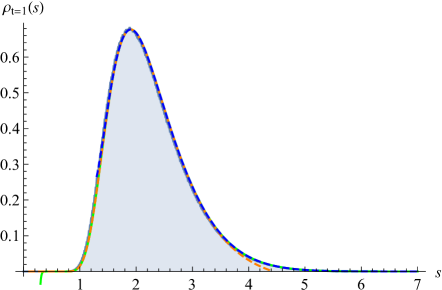
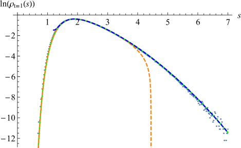
Figure 5: Left: The density of the span at time t=1𝑡1t=1. Grey: RW simulation with δt=104𝛿𝑡superscript104\delta t=10^{-4}, and 106superscript10610^{6} samples. Green: the analytic result (47). Orange dashed the small-s𝑠s asymptotics (48); blue dashed the large-s𝑠s asymptotics (49). Right: ibid. on a log-scale.

Inserting the definition (14) of \mathbb{P}, we get

PT1(t)subscript𝑃subscript𝑇1𝑡\displaystyle P_{T_{1}}(t) =\displaystyle= 4(1+2tt)n=e(2n+1)24ten2t4πt412𝑡subscript𝑡superscriptsubscript𝑛superscript𝑒superscript2𝑛124𝑡superscript𝑒superscript𝑛2𝑡4𝜋𝑡\displaystyle 4\big{(}1+2t\partial_{t}\big{)}\sum_{n=-\infty}^{\infty}\frac{e^{-\frac{(2n+1)^{2}}{4t}}-e^{-\frac{n^{2}}{t}}}{\sqrt{4\pi t}} (39)
=\displaystyle= 1πt3/2n=(2n+1)2e(2n+1)24t4n2en2t1𝜋superscript𝑡32superscriptsubscript𝑛superscript2𝑛12superscript𝑒superscript2𝑛124𝑡4superscript𝑛2superscript𝑒superscript𝑛2𝑡\displaystyle\frac{1}{\sqrt{\pi}t^{3/2}}\sum_{n=-\infty}^{\infty}(2n+1)^{2}e^{-\frac{(2n+1)^{2}}{4t}}-4n^{2}e^{-\frac{n^{2}}{t}}
=\displaystyle= 4tπt[ϑ2(0,e1/t)ϑ3(0,e1/t)].4𝑡𝜋subscript𝑡delimited-[]subscriptitalic-ϑ20superscript𝑒1𝑡subscriptitalic-ϑ30superscript𝑒1𝑡\displaystyle 4\sqrt{\frac{t}{\pi}}\partial_{t}\left[\vartheta_{2}\!\left(0,e^{-1/t}\right)-\vartheta_{3}\!\left(0,e^{-1/t}\right)\right]\ .

With the help of the Poisson-formula transformed Eq. (16), this can compactly be written as

PT1(t)=8n=0eπ2(2n+1)2t[2π2(2n+1)2t1].subscript𝑃subscript𝑇1𝑡8superscriptsubscript𝑛0superscript𝑒superscript𝜋2superscript2𝑛12𝑡delimited-[]2superscript𝜋2superscript2𝑛12𝑡1P_{T_{1}}(t)=8\sum_{n=0}^{\infty}e^{-\pi^{2}(2n+1)^{2}t}\left[2\pi^{2}(2n+1)^{2}t-1\right]\ . (40)

This result is compared to a numerical simulation on Fig. 4. Our expansions allow us to give simple formulas for the small and large-t𝑡t asymptotics,

PT1(t)subscript𝑃subscript𝑇1𝑡\displaystyle P_{T_{1}}(t) similar-to-or-equals\displaystyle\simeq 2e14tπt3/2+𝒪(e1t),2superscript𝑒14𝑡𝜋superscript𝑡32𝒪superscript𝑒1𝑡\displaystyle\frac{2e^{-\frac{1}{4t}}}{\sqrt{\pi}t^{3/2}}+{\cal O}(e^{-\frac{1}{t}})\ , (41)
PT1(t)subscript𝑃subscript𝑇1𝑡\displaystyle P_{T_{1}}(t) similar-to-or-equals\displaystyle\simeq eπ2t[16π2t8+𝒪(e8π2t)].superscript𝑒superscript𝜋2𝑡delimited-[]16superscript𝜋2𝑡8𝒪superscript𝑒8superscript𝜋2𝑡\displaystyle e^{-\pi^{2}t}\left[16\pi^{2}t-8+{\cal O}(e^{-8\pi^{2}t})\right]\ . (42)

These expansions work in a rather large, and overlapping domain, as can be seen on Fig. 4.

Its Laplace transform is

P~T1(s)subscript~𝑃subscript𝑇1𝑠\displaystyle\tilde{P}_{T_{1}}(s) =\displaystyle= 2(1+2ss)n=0dten2te(2n+1)24tπtest212𝑠subscript𝑠superscriptsubscript𝑛superscriptsubscript0differential-d𝑡superscript𝑒superscript𝑛2𝑡superscript𝑒superscript2𝑛124𝑡𝜋𝑡superscript𝑒𝑠𝑡\displaystyle 2(1+2s\partial_{s})\sum_{n=-\infty}^{\infty}\int_{0}^{\infty}\mathrm{d}t\,\frac{e^{-\frac{n^{2}}{t}}-e^{-\frac{(2n+1)^{2}}{4t}}}{\sqrt{\pi t}}\,e^{-st} (43)
=\displaystyle= 1cosh(s/2)2.\displaystyle\frac{1}{\cosh(\sqrt{s}/2)^{2}}\ .

Extracting the moments from the Laplace transform yields

T1=14,T12=112,T13=17480,formulae-sequencedelimited-⟨⟩subscript𝑇114formulae-sequencedelimited-⟨⟩superscriptsubscript𝑇12112delimited-⟨⟩superscriptsubscript𝑇1317480\left<T_{1}\right>=\frac{1}{4}\ ,\quad\left<T_{1}^{2}\right>=\frac{1}{12}\ ,\quad\left<T_{1}^{3}\right>=\frac{17}{480}\ ,\quad... (44)

Finally, let us connect to the classical work on the span Daniels1941 ; Feller1951 ; WeissRubin1976 ; PalleschiTorquati1989 . We will show how to reproduce formulas (3.7)-(3.8) in Feller1951 . The latter give the density ρt(s)subscript𝜌𝑡𝑠\rho_{t}(s) for the span s𝑠s at time t𝑡t. In our formalism, it can be obtained as

ρt(m2m1)=m1m2m1m2dxm1m2dy𝐏(x,y,m1,m2,t),subscript𝜌𝑡subscript𝑚2subscript𝑚1subscriptsubscript𝑚1subscriptsubscript𝑚2superscriptsubscriptsubscript𝑚1subscript𝑚2differential-d𝑥superscriptsubscriptsubscript𝑚1subscript𝑚2differential-d𝑦𝐏𝑥𝑦subscript𝑚1subscript𝑚2𝑡\rho_{t}(m_{2}-m_{1})=-\partial_{m_{1}}\partial_{m_{2}}\int\limits_{m_{1}}^{m_{2}}\mathrm{d}x\,\int\limits_{m_{1}}^{m_{2}}\mathrm{d}y\,\mathbf{P}(x,y,m_{1},m_{2},t)\ , (45)

where 𝐏(x,y,m1,m2,t)𝐏𝑥𝑦subscript𝑚1subscript𝑚2𝑡\mathbf{P}(x,y,m_{1},m_{2},t) is the probability to go from x𝑥x to y𝑦y in time t𝑡t, without being absorbed by the lower boundary positioned at m1subscript𝑚1m_{1}, or the upper boundary positioned at m2subscript𝑚2m_{2}. In terms of the propagator P+(x,y,t)subscript𝑃𝑥𝑦𝑡P_{+}(x,y,t), this can be written as

ρt(s)=s2[s01dx01dyP+(x,y,t/s2)].subscript𝜌𝑡𝑠superscriptsubscript𝑠2delimited-[]𝑠superscriptsubscript01differential-d𝑥superscriptsubscript01differential-d𝑦subscript𝑃𝑥𝑦𝑡superscript𝑠2\rho_{t}(s)=\partial_{s}^{2}\left[s\int\limits_{0}^{1}\mathrm{d}x\,\int\limits_{0}^{1}\mathrm{d}y\,P_{+}(x,y,t/s^{2})\right]\ . (46)

Using Eq. (15), and the series expansions (14) and (16) yields after integration and simplifications two different representations,

ρt(s)subscript𝜌𝑡𝑠\displaystyle\rho_{t}(s) =\displaystyle= 4πtn=1(1)n+1n2en2s24t4𝜋𝑡superscriptsubscript𝑛1superscript1𝑛1superscript𝑛2superscript𝑒superscript𝑛2superscript𝑠24𝑡\displaystyle\frac{4}{\sqrt{\pi t}}\sum_{n=1}^{\infty}(-1)^{n+1}n^{2}e^{-\frac{n^{2}s^{2}}{4t}} (47)
=\displaystyle= 16ts5n=0eπ2(2n+1)2ts2[2π2(2n+1)2ts2].16𝑡superscript𝑠5superscriptsubscript𝑛0superscript𝑒superscript𝜋2superscript2𝑛12𝑡superscript𝑠2delimited-[]2superscript𝜋2superscript2𝑛12𝑡superscript𝑠2\displaystyle\frac{16t}{s^{5}}\sum_{n=0}^{\infty}e^{-\frac{\pi^{2}(2n+1)^{2}t}{s^{2}}}\Big{[}2\pi^{2}(2n+1)^{2}t-s^{2}\Big{]}\ .\qquad

This is equivalent to Eqs. (3.7)-(3.8) in Feller1951 , if one there replaces t2t𝑡2𝑡t\to 2t. (Our covariance (2) at H=1/2𝐻12H=1/2 is 2t2𝑡2t instead of t𝑡t as in Feller1951 .) The small and large-s𝑠s asymptotics are

ρt(s)subscript𝜌𝑡𝑠\displaystyle\rho_{t}(s) similar-to-or-equals\displaystyle\simeq 4πt[es24t4es2t+𝒪(e9s24t)],4𝜋𝑡delimited-[]superscript𝑒superscript𝑠24𝑡4superscript𝑒superscript𝑠2𝑡𝒪superscript𝑒9superscript𝑠24𝑡\displaystyle\frac{4}{\sqrt{\pi t}}\left[e^{-\frac{s^{2}}{4t}}-4e^{-\frac{s^{2}}{t}}+{\cal O}\Big{(}e^{-\frac{9s^{2}}{4t}}\Big{)}\right]\ , (48)
ρt(s)subscript𝜌𝑡𝑠\displaystyle\rho_{t}(s) similar-to-or-equals\displaystyle\simeq 16ts5eπ2ts2[2π2ts2]+𝒪(e9π2ts2).16𝑡superscript𝑠5superscript𝑒superscript𝜋2𝑡superscript𝑠2delimited-[]2superscript𝜋2𝑡superscript𝑠2𝒪superscript𝑒9superscript𝜋2𝑡superscript𝑠2\displaystyle\frac{16t}{s^{5}}e^{-\frac{\pi^{2}t}{s^{2}}}\Big{[}2\pi^{2}t-s^{2}\Big{]}+{\cal O}\Big{(}e^{-\frac{9\pi^{2}t}{s^{2}}}\Big{)}\ .\qquad (49)

Note that in Eq. (48) we have also retained the subleading term for small s𝑠s, which considerably improves the numerical accuracy. A test is presented on Fig. 5.

III Corrections to the action for fBm

Here we briefly review the derivation of the effective action for fBm WieseMajumdarRosso2010 ; DelormeWiese2015 ; DelormeWiese2016 ; SadhuDelormeWiese2017 . The exact action for a Gaussian process with correlations 𝒞(t1,t2)𝒞subscript𝑡1subscript𝑡2{\cal C}(t_{1},t_{2}) is by definition

𝒮[X]𝒮delimited-[]𝑋\displaystyle{\cal S}[X] =\displaystyle= 0<t1<t2<TX˙t1𝒞1(t1,t2)X˙t2.subscript0subscript𝑡1subscript𝑡2𝑇subscript˙𝑋subscript𝑡1superscript𝒞1subscript𝑡1subscript𝑡2subscript˙𝑋subscript𝑡2\displaystyle\int_{0<t_{1}<t_{2}<T}\dot{X}_{t_{1}}{\cal C}^{-1}(t_{1},t_{2})\dot{X}_{t_{2}}\ . (50)

Here

𝒞(t1,t2)=X˙t1X˙t2𝒞subscript𝑡1subscript𝑡2delimited-⟨⟩subscript˙𝑋subscript𝑡1subscript˙𝑋subscript𝑡2\displaystyle{\cal C}(t_{1},t_{2})=\left<\dot{X}_{t_{1}}\dot{X}_{t_{2}}\right> (51)
=\displaystyle= 2δ(t1t2)2H|t2t1|2H12𝛿subscript𝑡1subscript𝑡22𝐻superscriptsubscript𝑡2subscript𝑡12𝐻1\displaystyle 2\delta(t_{1}-t_{2})2H|t_{2}-t_{1}|^{2H-1}
+2H(2H1)|t1t2|2(H1)2𝐻2𝐻1superscriptsubscript𝑡1subscript𝑡22𝐻1\displaystyle+2H(2H-1)|t_{1}-t_{2}|^{2(H-1)}
=\displaystyle= 2Dϵ[δ(t1t2)+ϵ|t1t2|+𝒪(ϵ2)].2subscript𝐷italic-ϵdelimited-[]𝛿subscript𝑡1subscript𝑡2italic-ϵsubscript𝑡1subscript𝑡2𝒪superscriptitalic-ϵ2\displaystyle 2D_{\epsilon}\left[\delta(t_{1}-t_{2})+\frac{\epsilon}{\left|t_{1}-t_{2}\right|}+{\cal O}(\epsilon^{2})\right]\ .

The diffusion constant, which depends on the small-time cutoff τ𝜏\tau implicit in the above construction, reads

Dϵ2Hτ2H1=(1+2ϵ)τ2ϵ.subscript𝐷italic-ϵ2𝐻superscript𝜏2𝐻112italic-ϵsuperscript𝜏2italic-ϵD_{\epsilon}\equiv 2H\tau^{2H-1}=(1+2\epsilon)\tau^{2\epsilon}\ . (52)

This scale can be understood as follows: Our procedure yields a random process Xtsubscript𝑋𝑡X_{t}, which is a Brownian process at times smaller than τ𝜏\tau, and an fBm at larger times.

The functional inverse of Eq. (51) which enters into the effective action (50) reads

𝒞1(t1,t2)=12Dϵ[δ(t1t2)ϵ|t1t2|+𝒪(ϵ2)].superscript𝒞1subscript𝑡1subscript𝑡212subscript𝐷italic-ϵdelimited-[]𝛿subscript𝑡1subscript𝑡2italic-ϵsubscript𝑡1subscript𝑡2𝒪superscriptitalic-ϵ2{\cal C}^{-1}(t_{1},t_{2})=\frac{1}{2D_{\epsilon}}\left[\delta(t_{1}-t_{2})-\frac{\epsilon}{\left|t_{1}-t_{2}\right|}+{\cal O}(\epsilon^{2})\right]. (53)

This allows us to write the action (50) as the action of Brownian motion, plus a non-local term

S[X]=𝒮0+ϵ𝒮1+𝒪(ϵ2),𝑆delimited-[]𝑋subscript𝒮0italic-ϵsubscript𝒮1𝒪superscriptitalic-ϵ2S[X]={\cal S}_{0}+\epsilon{\cal S}_{1}+{\cal O}(\epsilon^{2})\ , (54)

with

𝒮0subscript𝒮0\displaystyle{\cal S}_{0} :=14DϵtX˙t2assignabsent14subscript𝐷italic-ϵsubscript𝑡superscriptsubscript˙𝑋𝑡2\displaystyle:=\frac{1}{4D_{\epsilon}}\int_{t}\dot{X}_{t}^{2} (55)
𝒮1subscript𝒮1\displaystyle{\cal S}_{1} :=t1<t2δ𝒞1(t1,t2)X˙t1X˙t2.assignabsentsubscriptsubscript𝑡1subscript𝑡2𝛿superscript𝒞1subscript𝑡1subscript𝑡2subscript˙𝑋subscript𝑡1subscript˙𝑋subscript𝑡2\displaystyle:=\int_{t_{1}<t_{2}}\delta{\cal C}^{-1}(t_{1},t_{2})\dot{X}_{t_{1}}\dot{X}_{t_{2}}\ . (56)

Here δ𝒞1(t1,t2)𝛿superscript𝒞1subscript𝑡1subscript𝑡2\delta{\cal C}^{-1}(t_{1},t_{2}) is the non-local part (t1t2subscript𝑡1subscript𝑡2t_{1}\neq t_{2}) of 𝒞1(t1,t2)superscript𝒞1subscript𝑡1subscript𝑡2{\cal C}^{-1}(t_{1},t_{2}) defined in Eq. (53).

We will use the trick to represent the propagator as |t|1=y>0ey|t|superscript𝑡1subscript𝑦0superscript𝑒𝑦𝑡|t|^{-1}=\int_{y>0}e^{-y|t|}, which allows us to treat a small-time cutoff τ𝜏\tau for a momentum cutoff ΛΛ\Lambda. The relation between these two cutoffs can be inferred from

0Tdt0Λeytdy=ln(TΛ)+γE+𝒪(eTΛ)superscriptsubscript0𝑇differential-d𝑡superscriptsubscript0Λsuperscript𝑒𝑦𝑡differential-d𝑦𝑇Λsubscript𝛾E𝒪superscript𝑒𝑇Λ\displaystyle\int_{0}^{T}\mathrm{d}t\int_{0}^{\Lambda}e^{-yt}\mathrm{d}y=\ln(T\Lambda)+\gamma_{\rm E}+{\cal O}(e^{-T\Lambda})
=!ln(T/τ)=τTdtt.superscriptabsent𝑇𝜏superscriptsubscript𝜏𝑇d𝑡𝑡\displaystyle\qquad\stackrel{{\scriptstyle!}}{{=}}\ln(T/\tau)=\int_{\tau}^{T}\frac{\mathrm{d}t}{t}\ . (57)

This implies that up to exponentially small terms

Λ=eγEτ.Λsuperscript𝑒subscript𝛾E𝜏\Lambda=\frac{e^{-\gamma_{\rm E}}}{\tau}\ . (58)

IV The absorption current at 1-loop order

IV.1 General formulas

We want to calculate the current at the upper boundary at time t𝑡t, when starting at x𝑥x at time 0. We denote this by calligraphic 𝒥(x,1,t)𝒥𝑥1𝑡{\cal J}(x,1,t), to distinguish it from the Brownian result J(x,1,t)𝐽𝑥1𝑡J(x,1,t). We follow the procedure outlined in Ref. DelormeWiese2016 , which works on the Laplace-transformed version. The outgoing current at order ϵitalic-ϵ\epsilon reads

𝒥~(x,1,s)=J~(x,1,sDϵ)+2ϵ𝒜~(x,s)+𝒪(ϵ2)~𝒥𝑥1𝑠~𝐽𝑥1𝑠subscript𝐷italic-ϵ2italic-ϵ~𝒜𝑥𝑠𝒪superscriptitalic-ϵ2\displaystyle\tilde{{\cal J}}(x,1,s)=\tilde{J}\Big{(}x,1,\frac{s}{D_{\epsilon}}\Big{)}+2\epsilon\tilde{\cal A}(x,s)+{\cal O}(\epsilon^{2})
=J~(x,1,s)+2ϵ[𝒜~(x,s)(1+lnτ)ssJ~(x,1,s)]absent~𝐽𝑥1𝑠2italic-ϵdelimited-[]~𝒜𝑥𝑠1𝜏𝑠subscript𝑠~𝐽𝑥1𝑠\displaystyle=\tilde{J}(x,1,s)+2\epsilon\left[\tilde{\cal A}(x,s)-(1+\ln\tau)s\partial_{s}\tilde{J}(x,1,s)\right]
+𝒪(ϵ2).𝒪superscriptitalic-ϵ2\displaystyle~{}~{}~{}+{\cal O}(\epsilon^{2})\ . (59)

(The relation for the currents in time has an additional factor of 1/Dϵ1subscript𝐷italic-ϵ1/D_{\epsilon}.) The first-order correction for the current at y=1𝑦1y=1 is

𝒜~(x,s)=0Λdy~𝒜𝑥𝑠superscriptsubscript0Λdifferential-d𝑦\displaystyle\tilde{\cal A}(x,s)=\int_{0}^{\Lambda}\mathrm{d}y 01dx101dx2P~+(x,x1,s)superscriptsubscript01differential-dsubscript𝑥1superscriptsubscript01differential-dsubscript𝑥2subscript~𝑃𝑥subscript𝑥1𝑠\displaystyle\int_{0}^{1}\mathrm{d}x_{1}\int_{0}^{1}\mathrm{d}x_{2}\,\tilde{P}_{+}(x,x_{1},s)
×x1P~+(x1,x2,s+y)x2J~(x2,1,s).\displaystyle\times\partial_{x_{1}}\tilde{P}_{+}(x_{1},x_{2},s+y)\,\partial_{x_{2}}\tilde{J}(x_{2},1,s)\ .

The resulting expression after integration over x1subscript𝑥1x_{1} and x2subscript𝑥2x_{2} is rather lengthy, but can be simplified to

𝒜~(x,s)~𝒜𝑥𝑠\displaystyle\!\!\!\tilde{\cal A}(x,s) =\displaystyle= 0Λdys2y2sinh(s+y)sinh(s)×\displaystyle\int_{0}^{\Lambda}\mathrm{d}y\,\frac{\sqrt{s}}{2y^{2}\sinh(\sqrt{s+y}){\text{sinh}(\sqrt{s})}}\times (61)
×[sinh(sx)sinh(s)(s+y(34cosh(s)cosh(s+y)+cosh(2s))+ycosh(s)sinh(s+y))\displaystyle~{}~{}~{}~{}\times\bigg{[}\frac{\sinh(\sqrt{s}x)}{\text{sinh}(\sqrt{s})}\bigg{(}\sqrt{s+y}\Big{(}3-4\cosh(\sqrt{s})\cosh(\sqrt{s+y})+\cosh(2\sqrt{s})\Big{)}+y\cosh\left(\sqrt{s}\right)\sinh\left(\sqrt{s+y}\right)\bigg{)}
cosh(sx)(xysinh(s+y)+2s+y(cosh(s)cosh(s+y)))𝑠𝑥𝑥𝑦𝑠𝑦2𝑠𝑦𝑠𝑠𝑦\displaystyle~{}~{}~{}~{}~{}~{}~{}~{}~{}~{}~{}~{}-{\cosh(\sqrt{s}x)}\bigg{(}xy\sinh\left(\sqrt{s+y}\right)+2\sqrt{s+y}\Big{(}\cosh(\sqrt{s})-\cosh(\sqrt{s+y})\Big{)}\bigg{)}
2s+ycosh((1x)s+y)+2s+ycosh(s)cosh(xs+y)].\displaystyle~{}~{}~{}~{}~{}~{}~{}~{}~{}~{}~{}~{}-2\sqrt{s+y}{\,\cosh\Big{(}(1-x)\sqrt{s+y}\Big{)}}+2\sqrt{s+y}\cosh\left(\sqrt{s}\right)\cosh\left(x\sqrt{s+y}\right)\bigg{]}\ .

As the integrand vanishes at x=0𝑥0x=0 and x=1𝑥1x=1,

A~(0,s)=A~(1,s)=0.~𝐴0𝑠~𝐴1𝑠0\tilde{A}(0,s)=\tilde{A}(1,s)=0\ . (62)

The integral (61) is difficult to integrate analytically – or numerically. We will therefore study moments of s𝑠s, which allow us to access the exit probability, and the first moments of the exit times. We start with the lowest moment, the exit probability.

IV.2 Absorption probability at the upper boundary

The limit of s0𝑠0s\to 0 in the integral (61) yields the correction to the probability to exit at the upper boundary, starting at x𝑥x. Simplifying Eq. (61), we find

𝒜~(x,0)~𝒜𝑥0\displaystyle\tilde{\cal A}(x,0) =\displaystyle= 0dyexy(2xexy+y+2xexy+exy+yexy+e2xyey)(ey+1)y3/2.superscriptsubscript0differential-d𝑦superscript𝑒𝑥𝑦2𝑥superscript𝑒𝑥𝑦𝑦2𝑥superscript𝑒𝑥𝑦superscript𝑒𝑥𝑦𝑦superscript𝑒𝑥𝑦superscript𝑒2𝑥𝑦superscript𝑒𝑦superscript𝑒𝑦1superscript𝑦32\displaystyle\int_{0}^{\infty}\mathrm{d}y\,\frac{e^{-x\sqrt{y}}\left(-2xe^{x\sqrt{y}+\sqrt{y}}+2xe^{x\sqrt{y}}+e^{x\sqrt{y}+\sqrt{y}}-e^{x\sqrt{y}}+e^{2x\sqrt{y}}-e^{\sqrt{y}}\right)}{\left(e^{\sqrt{y}}+1\right)y^{3/2}}\ . (63)

We set the cutoff ΛΛ\Lambda\to\infty, as the integral is convergent. The current at the lower boundary is by symmetry

A~(x,0)=A~(1x,0).~𝐴𝑥0~𝐴1𝑥0\tilde{A}(x,0)=-\tilde{A}(1-x,0)\ . (64)

To simplify this expression, we perform two variable transformations. The first sets y=z2𝑦superscript𝑧2y=z^{2}. The second z=ln(r)𝑧𝑟z=-\ln(r). This yields

𝒜~(x,0)=201drr1x+rx2rx+r+2x1r(r+1)ln2(r).~𝒜𝑥02superscriptsubscript01differential-d𝑟superscript𝑟1𝑥superscript𝑟𝑥2𝑟𝑥𝑟2𝑥1𝑟𝑟1superscript2𝑟\tilde{\cal A}(x,0)=-2\int_{0}^{1}\mathrm{d}r\,\frac{-r^{1-x}+r^{x}-2rx+r+2x-1}{r(r+1)\ln^{2}(r)}\ . (65)

This expression is still difficult to integrate, due to the logarithms in the denominator. Taking two derivatives simplifies this to
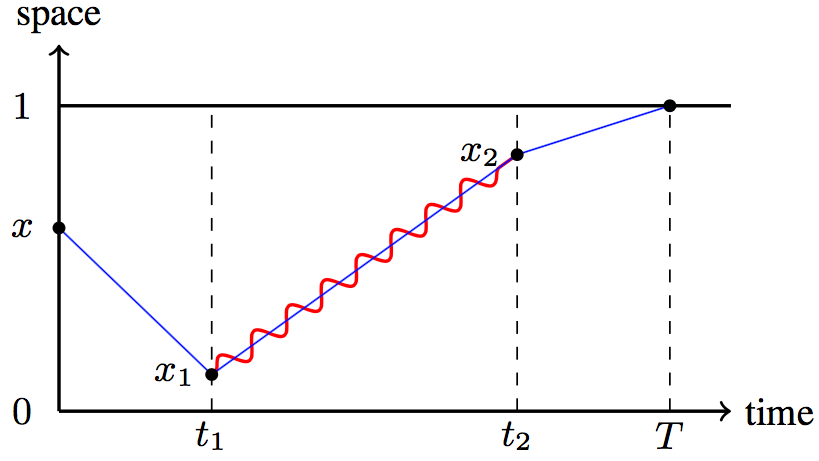
Refer to caption
Figure 6: Graphical representation of the path-integral for the order-ϵitalic-ϵ\epsilon contribution 𝒜~(x,s)~𝒜𝑥𝑠\tilde{\cal A}(x,s) given in Eq. (IV.1).
x2𝒜~(x,0)=201drrxrx1r+1superscriptsubscript𝑥2~𝒜𝑥02superscriptsubscript01differential-d𝑟superscript𝑟𝑥superscript𝑟𝑥1𝑟1\displaystyle\partial_{x}^{2}\,\tilde{\cal A}(x,0)=2\int_{0}^{1}\mathrm{d}r\,\frac{r^{-x}-r^{x-1}}{r+1} (66)
=\displaystyle= 2xψ(12x2)+ψ(1x2)ψ(x2+12)2𝑥𝜓12𝑥2𝜓1𝑥2𝜓𝑥212\displaystyle-\frac{2}{x}-\psi\!\left(\frac{1}{2}-\frac{x}{2}\right)+\psi\!\left(1-\frac{x}{2}\right)-\psi\!\left(\frac{x}{2}+\frac{1}{2}\right)
+ψ(x2+1).𝜓𝑥21\displaystyle+\psi\!\left(\frac{x}{2}+1\right)\ .

We now have to integrate twice w.r.t. x𝑥x, which gives the result plus terms of the form a+bx𝑎𝑏𝑥a+bx. The latter can be fixed by Eq. (62). The result is

𝒜~(x,0)~𝒜𝑥0\displaystyle\tilde{\cal A}(x,0) =\displaystyle= 13(2x1)[ln(2)3+36ζ(1)]132𝑥1delimited-[]2336superscript𝜁1\displaystyle\frac{1}{3}(2x-1)\Big{[}\ln(2)-3+36\zeta^{\prime}(-1)\Big{]} (67)
4ψ(2)(12x2)+4ψ(2)(1x2)4superscript𝜓212𝑥24superscript𝜓21𝑥2\displaystyle-4\psi^{(-2)}\!\left(\frac{1}{2}-\frac{x}{2}\right)+4\psi^{(-2)}\!\left(1-\frac{x}{2}\right)
+4ψ(2)(x2)4ψ(2)(x+12).4superscript𝜓2𝑥24superscript𝜓2𝑥12\displaystyle+4\psi^{(-2)}\!\left(\frac{x}{2}\right)-4\psi^{(-2)}\!\left(\frac{x+1}{2}\right)\ .

For P1(x)superscriptsubscript𝑃1𝑥P_{1}^{\prime}(x), we also need its first derivative

x𝒜~(x,0)=2subscript𝑥~𝒜𝑥02\displaystyle\partial_{x}\tilde{\cal A}(x,0)=2 [[\displaystyle\bigg{[} 12ζ(1)+ln(2)3+ln(Γ(12x2))12superscript𝜁123Γ12𝑥2\displaystyle 12\zeta^{\prime}(-1)+\frac{\ln(2)}{3}+\ln\!\bigg{(}\Gamma\Big{(}\frac{1}{2}-\frac{x}{2}\Big{)}\bigg{)} (68)
ln(Γ(1x2))+ln(Γ(x2))Γ1𝑥2Γ𝑥2\displaystyle-\ln\!\bigg{(}\Gamma\Big{(}1-\frac{x}{2}\Big{)}\bigg{)}+\ln\!\bigg{(}\Gamma\Big{(}\frac{x}{2}\Big{)}\bigg{)}
ln(Γ(x+12))].\displaystyle-\ln\!\bigg{(}\Gamma\Big{(}\frac{x+1}{2}\Big{)}\bigg{)}\bigg{]}\ .

The Taylor expansion of A~(x,0)~𝐴𝑥0\tilde{A}(x,0) is

𝒜~(x,0)~𝒜𝑥0\displaystyle\tilde{\cal A}(x,0) =\displaystyle= x[2ln(x)+83(9ζ(1)+ln(2))]𝑥delimited-[]2𝑥839superscript𝜁12\displaystyle x\left[-2\ln(x)+\frac{8}{3}\Big{(}9\zeta^{\prime}(-1)+\ln(2)\Big{)}\right] (69)
+x2ln(4)+x4ζ(3)4+x6ζ(5)8+9x8ζ(7)128superscript𝑥24superscript𝑥4𝜁34superscript𝑥6𝜁589superscript𝑥8𝜁7128\displaystyle+x^{2}\ln(4)+\frac{x^{4}\zeta(3)}{4}+\frac{x^{6}\zeta(5)}{8}+\frac{9x^{8}\zeta(7)}{128}
+17x10ζ(9)384+𝒪(x12).17superscript𝑥10𝜁9384𝒪superscript𝑥12\displaystyle+\frac{17x^{10}\zeta(9)}{384}+{\cal O}(x^{12})\ .

Note the logarithmic term, which can be interpreted as a correction to the power law for x0𝑥0x\to 0 in P1(x)subscriptsuperscript𝑃1𝑥P^{\prime}_{1}(x). Indeed, scaling suggests WieseMajumdarRosso2010 ; MajumdarRossoZoia2010b ; DelormeWiese2016

𝒫1,scaling(x)=[x(1x)]1H2Γ(2H2)Γ(1H1)2.superscriptsubscript𝒫1scaling𝑥superscriptdelimited-[]𝑥1𝑥1𝐻2Γ2𝐻2Γsuperscript1𝐻12{\cal P}_{\rm 1,scaling}^{\prime}(x)=[x(1-x)]^{\frac{1}{H}-2}\frac{\Gamma\big{(}\frac{2}{H}-2\big{)}}{\Gamma\big{(}\frac{1}{H}-1\big{)}^{2}}\ . (70)

​​(a)Refer to caption

T(x)subscript𝑇𝑥{\cal F}_{T}(x)

x𝑥x
             (b)​​ Refer to caption

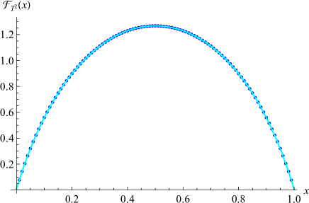
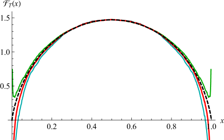
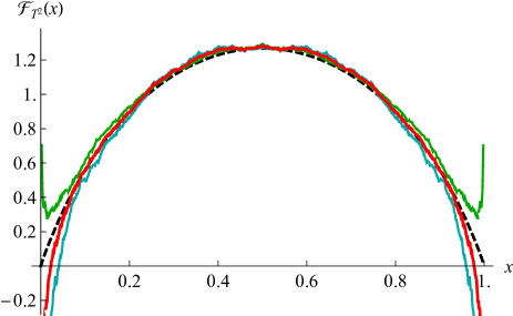
Figure 7: (a) The function T(x)subscript𝑇𝑥{\cal F}_{T}(x), defined in Eq. (IV.4). (b) The function T2(x)subscriptsuperscript𝑇2𝑥{\cal F}_{T^{2}}(x), defined in Eq. (89). The dots are the numerically obtained points, the line the fit of Eq. (90).

The correction to Eq. (70) at order ϵitalic-ϵ\epsilon can be written as

𝒫1(x)superscriptsubscript𝒫1𝑥\displaystyle{\cal P}_{1}^{\prime}(x) =\displaystyle= 𝒩[x(1x)]1H2eϵ(x),𝒩superscriptdelimited-[]𝑥1𝑥1𝐻2superscript𝑒italic-ϵ𝑥\displaystyle{\cal N}[x(1-x)]^{\frac{1}{H}-2}e^{\epsilon{\cal F}(x)}\ , (71)
(x)𝑥\displaystyle{\cal F}(x) =\displaystyle= 2x𝒜~(x,0)+4ln(x)+4ln(1x)+82subscript𝑥~𝒜𝑥04𝑥41𝑥8\displaystyle 2\partial_{x}\tilde{\cal A}(x,0)+4\ln(x)+4\ln(1-x)+8 (72)
=\displaystyle= 4[12ζ(1)+ln(2)3+ln(x(1x))\displaystyle 4\bigg{[}12\zeta^{\prime}(-1)+\frac{\ln(2)}{3}+\ln\big{(}x(1-x)\big{)}
+ln(Γ(12x2))ln(Γ(1x2))Γ12𝑥2Γ1𝑥2\displaystyle~{}~{}~{}+\ln\!\bigg{(}\!\Gamma\!\Big{(}{\frac{1}{2}-\frac{x}{2}}\Big{)}\!\bigg{)}-\ln\!\bigg{(}\!\Gamma\!\Big{(}1-\frac{x}{2}\Big{)}\!\bigg{)}
+ln(Γ(x2))ln(Γ(x+12))].\displaystyle~{}~{}~{}+\ln\!\bigg{(}\!\Gamma\!\Big{(}\frac{x}{2}\Big{)}\!\bigg{)}-\ln\!\bigg{(}\!\Gamma\!\Big{(}\frac{x+1}{2}\Big{)}\!\bigg{)}\bigg{]}\ .

We have chosen conventions s.t. 01dx(x)=0superscriptsubscript01differential-d𝑥𝑥0\int_{0}^{1}\mathrm{d}x\,{\cal F}(x)=0, moving the constant term into the normalization 𝒩𝒩{\cal N}. The latter has to be chosen such that 01dx𝒫1(x)=1superscriptsubscript01differential-d𝑥superscriptsubscript𝒫1𝑥1\int_{0}^{1}\mathrm{d}x\,{\cal P}_{1}^{\prime}(x)=1. The function (x)𝑥{\cal F}(x) is plotted on Fig. 2. It has a regular Taylor expansion around x=0𝑥0x=0,

(x)𝑥\displaystyle{\cal F}(x) =\displaystyle= 43[36ζ(1)+3+4ln(2)]+x(ln(256)4)2x243delimited-[]36superscript𝜁1342𝑥25642superscript𝑥2\displaystyle\frac{4}{3}\left[36\zeta^{\prime}(-1)+3+4\ln(2)\right]+x(\ln(256)-4)-2x^{2} (73)
+23x3(3ζ(3)2)x4+110x5(15ζ(5)8)23superscript𝑥33𝜁32superscript𝑥4110superscript𝑥515𝜁58\displaystyle+\frac{2}{3}x^{3}(3\zeta(3)-2)-x^{4}+\frac{1}{10}x^{5}(15\zeta(5)-8)
+𝒪(x6).𝒪superscript𝑥6\displaystyle+{\cal O}(x^{6})\ .

For numerical purposes, a Taylor expansion around x=1/2𝑥12x=1/2 is appropriate (with error <0.002absent0.002<0.002)

(x)𝑥\displaystyle{\cal F}(x) =\displaystyle= 48ζ(1)8lnΓ(34)+8lnΓ(14)+4203ln(2)48superscript𝜁18lnΓ348lnΓ1442032\displaystyle 48\zeta^{\prime}(-1)-8\text{ln$\Gamma$}({\textstyle\frac{3}{4}})+8\text{ln$\Gamma$}({\textstyle\frac{1}{4}})+4-{\textstyle\frac{20}{3}}\ln(2) (74)
+16(C1)(x12)216𝐶1superscript𝑥122\displaystyle+16(C-1)(x-{\textstyle\frac{1}{2}})^{2}
+148(x12)4[ψ(3)(14)ψ(3)(34)1536]148superscript𝑥124delimited-[]superscript𝜓314superscript𝜓3341536\displaystyle\textstyle+\frac{1}{48}(x-{\textstyle\frac{1}{2}})^{4}\left[\psi^{(3)}({\textstyle\frac{1}{4}})-\psi^{(3)}({\textstyle\frac{3}{4}})-1536\right]
+𝒪(x12)6𝒪superscript𝑥126\displaystyle+{\cal O}({\textstyle x-\frac{1}{2}})^{6}
=\displaystyle= 0.1167361.34455(x12)20.353774(x12)40.1167361.34455superscript𝑥1220.353774superscript𝑥124\displaystyle 0.116736-1.34455(x-{\textstyle\frac{1}{2}})^{2}-0.353774(x-{\textstyle\frac{1}{2}})^{4}
+𝒪(x12)6.𝒪superscript𝑥126\displaystyle+{\cal O}({\textstyle x-\frac{1}{2}})^{6}\ .

Validation of this function via a numerical simulation is given on Figs. 13 and 14.

IV.3 Remark on resummation

In Eq. (71), we had written the scaling function (x)𝑥{\cal F}(x) in the exponential. Since our calculation is performed at first order in ϵitalic-ϵ\epsilon, other forms are possible,

𝒫1(x)superscriptsubscript𝒫1𝑥\displaystyle{\cal P}_{1}^{\prime}(x) =\displaystyle= 𝒩[x(1x)]1H2eϵ(x)+𝒪(ϵ2)𝒩superscriptdelimited-[]𝑥1𝑥1𝐻2superscript𝑒italic-ϵ𝑥𝒪superscriptitalic-ϵ2\displaystyle{\cal N}[x(1-x)]^{\frac{1}{H}-2}e^{\epsilon{\cal F}(x)}+{\cal O}(\epsilon^{2}) (75)
=\displaystyle= 𝒩[x(1x)]1H2[1+ϵ(x)]+𝒪(ϵ2)𝒩superscriptdelimited-[]𝑥1𝑥1𝐻2delimited-[]1italic-ϵ𝑥𝒪superscriptitalic-ϵ2\displaystyle{\cal N}[x(1-x)]^{\frac{1}{H}-2}\big{[}1+\epsilon{\cal F}(x)\big{]}+{\cal O}(\epsilon^{2})\qquad (76)
=\displaystyle= 𝒩[x(1x)]1H211ϵ(x)+𝒪(ϵ2)𝒩superscriptdelimited-[]𝑥1𝑥1𝐻211italic-ϵ𝑥𝒪superscriptitalic-ϵ2\displaystyle{\cal N}[x(1-x)]^{\frac{1}{H}-2}\frac{1}{1-\epsilon{\cal F}(x)}+{\cal O}(\epsilon^{2})
=\displaystyle= \displaystyle...

The question arises which one to choose. There are many good reasons to choose the form (75):

  1. 1.

    adding drift μ𝜇\mu to Browian motion, the latter appears as an additive term in the exponential

    P+μ(x,y,t)=eμ(yx)2μ2t4P+(x,y,t).subscriptsuperscript𝑃𝜇𝑥𝑦𝑡superscript𝑒𝜇𝑦𝑥2superscript𝜇2𝑡4subscript𝑃𝑥𝑦𝑡P^{\mu}_{+}(x,y,t)=e^{\frac{\mu(y-x)}{2}-\frac{\mu^{2}t}{4}}P_{+}(x,y,t)\ . (78)
  2. 2.

    the first-order correction (68) contains logarithmic terms, visible in Eq. (69). Having them in the exponential, they are resummed into power laws, according to

    eϵln(x)=xϵ.superscript𝑒italic-ϵ𝑥superscript𝑥italic-ϵe^{\epsilon\ln(x)}=x^{\epsilon}. (79)

    This is how in Eq. (71) the scaling function of the Brownian, x(1x)𝑥1𝑥x(1-x), was changed into [x(1x)]1H1superscriptdelimited-[]𝑥1𝑥1𝐻1[x(1-x)]^{\frac{1}{H}-1}. At the same time, the scaling function (x)𝑥{\cal F}(x), defined in Eq. (72), becomes regular for x0𝑥0x\to 0, as can be seen on Eq. (73).

  3. 3.

    in field theory, perturbative corrections are in general, and most efficiently, calculated for the effective action, i.e. the log of the partition function. In a thermodynamic setting as the one here, the effective action can be interpreted as the free energy.

  4. 4.

    Finally, as the exponential function is always positive for real arguments, the form (75) remains positive even when ϵ(x)italic-ϵ𝑥\epsilon{\cal F}(x) becomes large. This is a necessary condition for a probability density.

For all these reasons, using the exponentiated version is the most natural choice, and the one chosen throughout this article. When corrections are large, which is especially important for universal amplitudes, we will compare this choice with the linear extrapolation (76).

IV.4 Expectation of exit time

The non-trivial 1-loop correction to Texit(x)delimited-⟨⟩subscript𝑇exit𝑥\left<T_{\rm exit}(x)\right> given in Eq. (28) is 2ϵ2italic-ϵ2\epsilon times

(x):=s[𝒜~(x,s)+𝒜~(1x,s)]|s=0.assign𝑥evaluated-atsubscript𝑠delimited-[]~𝒜𝑥𝑠~𝒜1𝑥𝑠𝑠0{\cal B}(x):=-\partial_{s}\left[\tilde{\cal A}(x,s)+\tilde{\cal A}(1-x,s)\right]\Big{|}_{s=0}\ . (80)

Note that this combination is much simpler than the unsymmetrized one, which will allow us to integrate it analytically. We find with the same variable transformations as above

(x)=eΛ1dr[1r(1rx11+11rx)ln2(r)+(1x)xrln(r)].𝑥superscriptsubscriptsuperscript𝑒Λ1differential-d𝑟delimited-[]1𝑟1superscript𝑟𝑥1111superscript𝑟𝑥superscript2𝑟1𝑥𝑥𝑟𝑟{\cal B}(x)=\int\limits_{e^{-\sqrt{\Lambda}}}^{1}\mathrm{d}r\left[\frac{1}{r\left(\frac{1}{r^{x-1}-1}+\frac{1}{1-r^{x}}\right)\ln^{2}(r)}+\frac{(1-x)x}{r\ln(r)}\right]. (81)

Both terms can be integrated, the first after taking two derivatives w.r.t. x𝑥x. Integrating twice w.r.t. x𝑥x, and fixing the lost terms of the form a+bx𝑎𝑏𝑥a+bx by demanding, according to Eq. (62), that (0)=(1)=0010{\cal B}(0)={\cal B}(1)=0 yields111Note that there are corrections in the boundary region of the form eΛx/xsuperscript𝑒Λ𝑥𝑥e^{-\sqrt{\Lambda}x}/x. These might be interpreted as the finite-discretization corrections seen in the simulations of section V. We did not try to make this statement quantitative.

(x)𝑥\displaystyle{\cal B}(x) =\displaystyle= [γE(x1)+1]xxln(x)+12(x1)xln(Λ)delimited-[]subscript𝛾E𝑥11𝑥𝑥𝑥12𝑥1𝑥Λ\displaystyle\left[\gamma_{\rm E}(x-1)+1\right]x-x\ln(x)+\frac{1}{2}(x-1)x\ln(\Lambda) (82)
+ψ(2)(1x)+ψ(2)(x+1)ln(2π).superscript𝜓21𝑥superscript𝜓2𝑥12𝜋\displaystyle+\psi^{(-2)}(1-x)+\psi^{(-2)}(x+1)-\ln(2\pi)\ .

Taylor-expanding for small x(1x)𝑥1𝑥x(1-x), we find

2ϵ(x)Texit(x)02italic-ϵ𝑥subscriptdelimited-⟨⟩subscript𝑇exit𝑥0\displaystyle\frac{2\epsilon{\cal B}(x)}{\left<T_{\rm exit}(x)\right>_{0}} =\displaystyle= 4ϵ[γE1+ln(x(1x)Λ)]4italic-ϵdelimited-[]subscript𝛾E1𝑥1𝑥Λ\displaystyle-4\epsilon\left[\gamma_{\rm E}-1+\ln\!\Big{(}{x(1-x)}{\sqrt{\Lambda}}\Big{)}\right] (83)
+𝒪(x(1x)).𝒪𝑥1𝑥\displaystyle+{\cal O}\big{(}x(1-x)\big{)}\ .

This is consistent with

Texit(x)delimited-⟨⟩subscript𝑇exit𝑥\displaystyle\left<T_{\rm exit}(x)\right> =\displaystyle= 1DϵTexit(x)0+2ϵ(x)+𝒪(ϵ2)1subscript𝐷italic-ϵsubscriptdelimited-⟨⟩subscript𝑇exit𝑥02italic-ϵ𝑥𝒪superscriptitalic-ϵ2\displaystyle\frac{1}{D_{\epsilon}}\left<T_{\rm exit}(x)\right>_{0}+2\epsilon{\cal B}(x)+{\cal O}(\epsilon^{2}) (84)
similar-to\displaystyle\sim [x(1x)]1H1+𝒪(ϵ2).superscriptdelimited-[]𝑥1𝑥1𝐻1𝒪superscriptitalic-ϵ2\displaystyle[x(1-x)]^{\frac{1}{H}-1}+{\cal O}(\epsilon^{2})\ .

Let us define

T(x):=2(x)Texit(x)0+4[ln(Λ(1x)x)+γE1]assignsubscript𝑇𝑥2𝑥subscriptdelimited-⟨⟩subscript𝑇exit𝑥04delimited-[]Λ1𝑥𝑥subscript𝛾E1\displaystyle\!\!{\cal F}_{T}(x):=\frac{2{\cal B}(x)}{\left<T_{\rm exit}(x)\right>_{0}}+4\left[\ln\!\Big{(}\sqrt{\Lambda}(1-x)x\Big{)}+\gamma_{\rm E}-1\right]
=4x(1x)[x2+x((1x)ln(1x)xln(x))\displaystyle=\frac{4}{x(1-x)}\Big{[}x^{2}+x\Big{(}(1-x)\ln(1-x)-x\ln(x)\Big{)}
+ψ(2)(1x)+ψ(2)(x+1)ln(2π)].\displaystyle~{}~{}~{}~{}~{}~{}~{}~{}~{}~{}~{}~{}~{}~{}~{}+\psi^{(-2)}(1-x)+\psi^{(-2)}(x+1)-\ln(2\pi)\Big{]}.~{}~{}~{} (85)

This function is plotted on Fig. 7 (left), and numerically validated in Fig. 8, and more precisely in Fig. 12.

IV.5 Expectation of exit time squared, Texit(x)2delimited-⟨⟩subscript𝑇exitsuperscript𝑥2\left<T_{\rm exit}(x)^{2}\right>

The first-order correction to Texit(x)2delimited-⟨⟩subscript𝑇exitsuperscript𝑥2\left<T_{\rm exit}(x)^{2}\right> given in Eq. (28) is 2ϵ2italic-ϵ2\epsilon times

𝒞(x):=s2[𝒜~(x,s)+𝒜~(1x,s)]|s=0.assign𝒞𝑥evaluated-atsuperscriptsubscript𝑠2delimited-[]~𝒜𝑥𝑠~𝒜1𝑥𝑠𝑠0{\cal C}(x):=\partial_{s}^{2}\left[\tilde{\cal A}(x,s)+\tilde{\cal A}(1-x,s)\right]\Big{|}_{s=0}\ . (86)

Again, this combination is much simpler than the unsymmetrized one. We find with the same variable transformations as above

𝒞(x)𝒞𝑥\displaystyle{\cal C}(x) =\displaystyle= eΛ1dr[1r(rrrx+1rx1)ln4(r)\displaystyle\int_{e^{-\sqrt{\Lambda}}}^{1}\mathrm{d}r\,\Bigg{[}\frac{1}{r\left(\frac{r}{r-r^{x}}+\frac{1}{r^{x}-1}\right)\ln^{4}(r)} (87)
+xr1x+xrx1xrx+rxxrx+rx2(r1)2ln3(r)𝑥superscript𝑟1𝑥𝑥superscript𝑟𝑥1𝑥superscript𝑟𝑥superscript𝑟𝑥𝑥superscript𝑟𝑥superscript𝑟𝑥2superscript𝑟12superscript3𝑟\displaystyle+\frac{xr^{1-x}+xr^{x-1}-xr^{-x}+r^{-x}-xr^{x}+r^{x}-2}{(r-1)^{2}\ln^{3}(r)}
+r1x+rx+(r+1)(6(x1)x1)6(r1)rln2(r)superscript𝑟1𝑥superscript𝑟𝑥𝑟16𝑥1𝑥16𝑟1𝑟superscript2𝑟\displaystyle+\frac{r^{1-x}+r^{x}+(r+1)(6(x-1)x-1)}{6(r-1)r\ln^{2}(r)}
+x42x3+x3rln(r)].\displaystyle+\frac{x^{4}-2x^{3}+x}{3r\ln(r)}\Bigg{]}\ .

Anticipating that a good approximation is given by T2(x)[Texit2(x)0]1H1similar-todelimited-⟨⟩superscript𝑇2𝑥superscriptdelimited-[]subscriptdelimited-⟨⟩superscriptsubscript𝑇exit2𝑥01𝐻1\left<T^{2}(x)\right>\sim\left[\left<T_{\rm exit}^{2}(x)\right>_{0}\right]^{\frac{1}{H}-1}, we set with normalization 𝒩𝒩{\cal N}

Texit2(x)=𝒩[Texit2(x)0]1H1eϵT2(x)+𝒪(ϵ2).delimited-⟨⟩superscriptsubscript𝑇exit2𝑥𝒩superscriptdelimited-[]subscriptdelimited-⟨⟩superscriptsubscript𝑇exit2𝑥01𝐻1superscript𝑒italic-ϵsubscriptsuperscript𝑇2𝑥𝒪superscriptitalic-ϵ2\left<T_{\rm exit}^{2}(x)\right>={\cal N}\left[\left<T_{\rm exit}^{2}(x)\right>_{0}\right]^{\frac{1}{H}-1}e^{\epsilon{\cal F}_{T^{2}}(x)+{\cal O}(\epsilon^{2})}\ . (88)

This implies that up to a constant, which will notably depend on the UV-cutoff ΛΛ\Lambda,

T2(x)=2𝒞(X)+4ln(Texit2(x)0)+constsubscriptsuperscript𝑇2𝑥2𝒞𝑋4subscriptdelimited-⟨⟩superscriptsubscript𝑇exit2𝑥0const\displaystyle\!\!\!\!\!\!\!{{\cal F}_{T^{2}}(x)=2\,{\cal C}(X)+4\ln\big{(}\left<T_{\rm exit}^{2}(x)\right>_{0}\big{)}+\mbox{const}} (89)
=\displaystyle= 2𝒞(X)+4ln(x(1x)(1+xx2))+const.2𝒞𝑋4𝑥1𝑥1𝑥superscript𝑥2const\displaystyle 2\,{\cal C}(X)+4\ln\big{(}x(1-x)(1+x-x^{2})\big{)}+\mbox{const}\ .\qquad

We did not succeed to integrate Eq. (87) analytically. A numerical integration can be done without difficulty, and yields the points on Fig. 7 (right). A fit with a symmetric polynomial of degree 8 (with a total systematic plus numerical deviation smaller than 103superscript10310^{-3}) reads

T2(x)subscriptsuperscript𝑇2𝑥\displaystyle{\cal F}_{T^{2}}(x) \displaystyle\approx 1.260333.73328(x12)24.16628(x12)41.260333.73328superscript𝑥1224.16628superscript𝑥124\displaystyle\textstyle 1.26033-3.73328\left(x-\frac{1}{2}\right)^{2}-4.16628\left(x-\frac{1}{2}\right)^{4} (90)
+5.24129(x12)638.0198(x12)8.5.24129superscript𝑥12638.0198superscript𝑥128\displaystyle\textstyle+5.24129\left(x-\frac{1}{2}\right)^{6}-38.0198\left(x-\frac{1}{2}\right)^{8}\ .

Validation via a numerical simulation is presented on Fig. 12.

IV.6 Estimation of time scales: The mean exit time

Up to now, we considered universal functions, without explicit evaluation of the proper time scales. This is motivated by the observation that time scales are often more sensitive to details of the implementation than amplitude ratios, as those encoded in the functions (x)𝑥{\cal F}(x), T(x)subscript𝑇𝑥{\cal F}_{T}(x), and T2(x)subscriptsuperscript𝑇2𝑥{\cal F}_{T^{2}}(x). Nevertheless, our formalism is able to compute universal amplitudes, a task we turn to now.

We start by the simplest such observable, the mean exit time in the strip. By mean we understand an average over the starting position x𝑥x, and the realization of the process. According to Eqs. (28), (IV.1) and (80)

01Texit(x)dxsuperscriptsubscript01delimited-⟨⟩subscript𝑇exit𝑥differential-d𝑥\displaystyle\int_{0}^{1}\left<T_{\rm exit}(x)\right>\mathrm{d}x (91)
=s|s=001dx[J~(x,1,sDϵ)J~(x,0,sDϵ)]absentevaluated-atsubscript𝑠𝑠0superscriptsubscript01differential-d𝑥delimited-[]~𝐽𝑥1𝑠subscript𝐷italic-ϵ~𝐽𝑥0𝑠subscript𝐷italic-ϵ\displaystyle=-\partial_{s}\Big{|}_{s=0}\int_{0}^{1}\mathrm{d}x\,\left[\tilde{J}\Big{(}x,1,\frac{s}{D_{\epsilon}}\Big{)}-\tilde{J}\Big{(}x,0,\frac{s}{D_{\epsilon}}\Big{)}\right]
+2ϵ[A~(x,s)A~(1x,s)]2italic-ϵdelimited-[]~𝐴𝑥𝑠~𝐴1𝑥𝑠\displaystyle\hphantom{=-\partial_{s}\Big{|}_{s=0}\int_{0}^{1}\mathrm{d}x}+2\epsilon\left[\tilde{A}(x,s)-\tilde{A}(1-x,s)\right]
=\displaystyle= 01x(1x)2Dϵ+2ϵ(x)dx.superscriptsubscript01𝑥1𝑥2subscript𝐷italic-ϵ2italic-ϵ𝑥d𝑥\displaystyle\int_{0}^{1}\frac{x(1-x)}{2D_{\epsilon}}+2\epsilon\,{\cal B}(x)\,\mathrm{d}x\ .

Recalling the definition of T(x)subscript𝑇𝑥{\cal F}_{T}(x) in Eq. (IV.4), this can be written as

01Texit(x)dxsuperscriptsubscript01delimited-⟨⟩subscript𝑇exit𝑥differential-d𝑥\displaystyle\int_{0}^{1}\left<T_{\rm exit}(x)\right>\mathrm{d}x (92)
=\displaystyle= 112Dϵ+ϵ201dxT(x)x(1x)112subscript𝐷italic-ϵitalic-ϵ2superscriptsubscript01differential-d𝑥subscript𝑇𝑥𝑥1𝑥\displaystyle\frac{1}{12D_{\epsilon}}+\frac{\epsilon}{2}\,\int_{0}^{1}\mathrm{d}x{\cal F}_{T}(x)x(1-x)
2ϵ01x(1x)[ln(Λx(1x))+γE1]dx.2italic-ϵsuperscriptsubscript01𝑥1𝑥delimited-[]Λ𝑥1𝑥subscript𝛾E1differential-d𝑥\displaystyle-2\epsilon\int_{0}^{1}x(1-x)\left[\ln(\sqrt{\Lambda}x(1-x))+\gamma_{\rm E}-1\right]\mathrm{d}x\ .~{}~{}~{}~{}~{}~{}~{}

The terms in question are

1201T(x)x(1x)dx=594ζ(1)=0.10612912superscriptsubscript01subscript𝑇𝑥𝑥1𝑥differential-d𝑥594superscript𝜁10.106129\displaystyle\frac{1}{2}\int_{0}^{1}{\cal F}_{T}(x)x(1-x)\,\mathrm{d}x=-\frac{5}{9}-4\zeta^{\prime}(-1)=0.106129...
(93)
201x(1x)[ln(Λx(1x))+γE1]dx2superscriptsubscript01𝑥1𝑥delimited-[]Λ𝑥1𝑥subscript𝛾E1differential-d𝑥\displaystyle-2\int_{0}^{1}x(1-x)\left[\ln(\sqrt{\Lambda}x(1-x))+\gamma_{\rm E}-1\right]\mathrm{d}x
=ln(Λ)6γE3+89=0.696484ln(Λ)6.absentΛ6subscript𝛾E3890.696484Λ6\displaystyle=-\frac{\ln(\Lambda)}{6}-\frac{\gamma_{\rm E}}{3}+\frac{8}{9}=0.696484...-\frac{\ln(\Lambda)}{6}\ . (94)

This yields

01Texit(x)dxsuperscriptsubscript01delimited-⟨⟩subscript𝑇exit𝑥differential-d𝑥\displaystyle\int_{0}^{1}\left<T_{\rm exit}(x)\right>\mathrm{d}x (95)
=112[1+2ϵ(1γE24ζ(1))+𝒪(ϵ2)]absent112delimited-[]12italic-ϵ1subscript𝛾E24superscript𝜁1𝒪superscriptitalic-ϵ2\displaystyle~{}~{}~{}=\frac{1}{12}\Big{[}1+2\epsilon\Big{(}1-\gamma_{\rm E}-24\zeta^{\prime}(-1)\Big{)}+{\cal O}(\epsilon^{2})\Big{]}
=112[1+8.78578ϵ+𝒪(ϵ2)]absent112delimited-[]18.78578italic-ϵ𝒪superscriptitalic-ϵ2\displaystyle~{}~{}~{}=\frac{1}{12}\Big{[}1+8.78578\epsilon+{\cal O}(\epsilon^{2})\Big{]}
=112exp(8.78578ϵ)+𝒪(ϵ2).absent1128.78578italic-ϵ𝒪superscriptitalic-ϵ2\displaystyle~{}~{}~{}=\frac{1}{12}\exp(8.78578\epsilon)+{\cal O}(\epsilon^{2})\ .

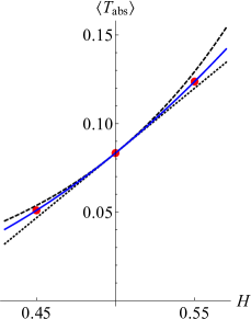
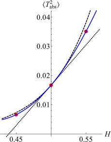
Note that all cutoff dependence has canceled, as expected. In the last two lines we gave two alternative resummations: The linear, order-ϵitalic-ϵ\epsilon term, and an exponential resummation, which was beneficial in resumming logarithms into a change in power-law. We will see later (Fig. 17) that the numerically obtained result lies between the two expressions.

IV.7 Exit times in the limit of x0𝑥0x\to 0

Another interesting limit is x0𝑥0x\to 0, also considered analytically in Ref. GuerinLevernierBenichouVoituriez2016 . Let us define the ratio

R(x):=Texit(x)[x(1x)]1H1.assign𝑅𝑥delimited-⟨⟩subscript𝑇exit𝑥superscriptdelimited-[]𝑥1𝑥1𝐻1R(x):=\frac{\left<T_{\rm exit}(x)\right>}{[x(1-x)]^{\frac{1}{H}-1}}\ . (96)

As in the preceding section, we derive for x0𝑥0x\to 0

R(0):=limx0R(x)=12+ϵ(1γE)+𝒪(ϵ2).assign𝑅0subscript𝑥0𝑅𝑥12italic-ϵ1subscript𝛾E𝒪superscriptitalic-ϵ2R(0):=\lim_{x\to 0}R(x)=\frac{1}{2}+\epsilon(1-\gamma_{\rm E})+{\cal O}(\epsilon^{2})\ . (97)

A test is given on Fig. 8. This limit agrees222Using in the supplementary material of GuerinLevernierBenichouVoituriez2016 ψ(t)=2Dt2H𝜓𝑡2𝐷superscript𝑡2𝐻\psi(t)=2Dt^{2H} yields ψ0(t)=2Dtsubscript𝜓0𝑡2𝐷𝑡\psi_{0}(t)=2Dt, and ψ1(t)=4Dtln(t)subscript𝜓1𝑡4𝐷𝑡𝑡\psi_{1}(t)=4Dt\ln(t). Eq. (G48) (generalized to arbitrary D𝐷D) becomes Tps(0)=x02D+ϵx0D(1γE2ln(x0)+4ln(D))+𝒪(ϵ2)𝑇subscript𝑝𝑠0subscript𝑥02𝐷italic-ϵsubscript𝑥0𝐷1subscript𝛾E2subscript𝑥04𝐷𝒪superscriptitalic-ϵ2Tp_{s}(0)=\frac{x_{0}}{2D}+\epsilon\frac{x_{0}}{D}(1-\gamma_{\rm E}-2\ln(x_{0})+4\ln(D))+{\cal O}(\epsilon^{2}). Setting D=1𝐷1D=1, we get limx0Tps(0)/x1H1=12+ϵ(1γE)subscript𝑥0𝑇subscript𝑝𝑠0superscript𝑥1𝐻112italic-ϵ1subscript𝛾E\lim_{x\to 0}Tp_{s}(0)/x^{\frac{1}{H}-1}=\frac{1}{2}+\epsilon(1-\gamma_{\rm E}), which agrees with R(0)𝑅0R(0) in Eq. 97. The order-ϵitalic-ϵ\epsilon correction extracted from the simulation data of Ref. GuerinLevernierBenichouVoituriez2016 is consistent with this value. with the equivalent object calculated in Ref. GuerinLevernierBenichouVoituriez2016 .
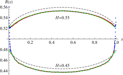
Refer to caption
Figure 8: The ratio R(x)𝑅𝑥{R(x)} defined in Eq. (96). In grey are the analytical (parameter free) predictions, in red or blue the data points of numerical simulations, presented in section V. The red data points have been used to extract via a polynomial fit of order 40 (dashed green line) R(0)𝑅0R(0), with the result RH=0.45num(0)=0.478superscriptsubscript𝑅𝐻0.45num00.478R_{H=0.45}^{\rm num}(0)=0.478, RH=0.55num(0)=0.522subscriptsuperscript𝑅num𝐻0.5500.522R^{\rm num}_{H=0.55}(0)=0.522. Analytically Eq. (97) yields RH=0.45ana(0)=0.479superscriptsubscript𝑅𝐻0.45ana00.479R_{H=0.45}^{\rm ana}(0)=0.479, RH=0.55ana(0)=0.521subscriptsuperscript𝑅ana𝐻0.5500.521R^{\rm ana}_{H=0.55}(0)=0.521. The deviation in the middle of the domain is of order 7×1037superscript1037\times 10^{-3}, consistent with an 𝒪(ϵ2)𝒪superscriptitalic-ϵ2{\cal O}(\epsilon^{2}) correction to R(x)𝑅𝑥R(x) of amplitude 3. More robust tests of our formulas, focusing on the shape of R(x)𝑅𝑥R(x), and the spatially averaged exit times, are presented in section V.3.

IV.8 Time scales: The second moment of the exit time

Analogously to the derivation of Eq. (91), we have

01Texit(x)2dxsuperscriptsubscript01delimited-⟨⟩subscript𝑇exitsuperscript𝑥2differential-d𝑥\displaystyle\int_{0}^{1}\left<T_{\rm exit}(x)^{2}\right>\mathrm{d}x (98)
=s2|s=001dx[J~(x,1,sDϵ)J~(x,0,sDϵ)]absentevaluated-atsuperscriptsubscript𝑠2𝑠0superscriptsubscript01differential-d𝑥delimited-[]~𝐽𝑥1𝑠subscript𝐷italic-ϵ~𝐽𝑥0𝑠subscript𝐷italic-ϵ\displaystyle=\partial_{s}^{2}\Big{|}_{s=0}\int_{0}^{1}\mathrm{d}x\,\left[\tilde{J}\big{(}x,1,\frac{s}{D_{\epsilon}}\Big{)}-\tilde{J}\Big{(}x,0,\frac{s}{D_{\epsilon}}\Big{)}\right]
+2ϵ[A~(x,s)A~(1x,s)]2italic-ϵdelimited-[]~𝐴𝑥𝑠~𝐴1𝑥𝑠\displaystyle\hphantom{=-\partial_{s}\Big{|}_{s=0}\int_{0}^{1}\mathrm{d}x}+2\epsilon\left[\tilde{A}(x,s)-\tilde{A}(1-x,s)\right]
=01x(1x)(1+xx2)12Dϵ2+2ϵ𝒞(x)dx.absentsuperscriptsubscript01𝑥1𝑥1𝑥superscript𝑥212superscriptsubscript𝐷italic-ϵ22italic-ϵ𝒞𝑥d𝑥\displaystyle=\int_{0}^{1}\frac{x(1-x)(1+x-x^{2})}{12D_{\epsilon}^{2}}+2\epsilon\,{\cal C}(x)\,\mathrm{d}x\ .

The first integral is

01x(1x)(1+xx2)12Dϵ2dx=160Dϵ2.superscriptsubscript01𝑥1𝑥1𝑥superscript𝑥212superscriptsubscript𝐷italic-ϵ2differential-d𝑥160superscriptsubscript𝐷italic-ϵ2\int_{0}^{1}\frac{x(1-x)(1+x-x^{2})}{12D_{\epsilon}^{2}}\mathrm{d}x=\frac{1}{60D_{\epsilon}^{2}}\ . (99)

The x𝑥x-integral over 𝒞(x)𝒞𝑥{\cal C}(x) defined in Eq. (87) can be done analytically. The remaining non-trivial integral reads

01𝒞(x)dxsuperscriptsubscript01𝒞𝑥differential-d𝑥\displaystyle\int\limits_{0}^{1}{\cal C}(x)\,\mathrm{d}x =eΛ1dr[r+13r(1r)ln2(r)+r+1(r1)rln4(r)\displaystyle=\int\limits_{e^{-\sqrt{\Lambda}}}^{1}\mathrm{d}r\bigg{[}\frac{r+1}{3r(1-r)\ln^{2}(r)}+\frac{r+1}{(r-1)r\ln^{4}(r)} (100)
+13r2(r1)2ln3(r)+115rln(r)].\displaystyle\hphantom{\int_{e^{-\sqrt{\Lambda}}}^{1}\mathrm{d}r}~{}~{}~{}+\frac{\frac{1}{3r}-\frac{2}{(r-1)^{2}}}{\ln^{3}(r)}+\frac{1}{15r\ln(r)}\bigg{]}.

This integral is hard to evaluate analytically. A precise numerical estimation can be obtained as follows: Taylor-expand the integral at small r𝑟r, and integrate, to show that

01𝒞(x)dxconst+13Λ3/213Λ+16Λln(Λ)30.similar-to-or-equalssuperscriptsubscript01𝒞𝑥differential-d𝑥const13superscriptΛ3213Λ16ΛΛ30\int\limits_{0}^{1}{\cal C}(x)\,\mathrm{d}x\simeq\mbox{const}+\frac{1}{3\Lambda^{3/2}}-\frac{1}{3\sqrt{\Lambda}}+\frac{1}{6\Lambda}-\frac{\ln(\Lambda)}{30}\ .~{}~{} (101)

The integral (100) can then be integrated numerically. To this aim, one splits it into two pieces: The region close to r=1𝑟1r=1, for which one Taylor-expands the integrand around r=1𝑟1r=1 and then integrates symbolically. And the remaining region, with cutoff ΛΛ\Lambda. Subtracting the terms in Eq. (101) from the numerically evaluated integral allows us to obtain the latter precisely already for relatively small ΛΛ\Lambda. The result of this procedure is

01𝒞(x)dx=0.152119ln(Λ)30+𝒪(1Λ).superscriptsubscript01𝒞𝑥differential-d𝑥0.152119Λ30𝒪1Λ\int\limits_{0}^{1}{\cal C}(x)\,\mathrm{d}x=0.152119\,-\frac{\ln(\Lambda)}{30}+{\cal O}\!\left(\frac{1}{\sqrt{\Lambda}}\right)\ . (102)

This yields for the second moment of the exit time

01Texit(x)2dxsuperscriptsubscript01delimited-⟨⟩subscript𝑇exitsuperscript𝑥2differential-d𝑥\displaystyle\int_{0}^{1}\left<T_{\rm exit}(x)^{2}\right>\mathrm{d}x =\displaystyle= 160[1+16.5632ϵ+𝒪(ϵ2)]160delimited-[]116.5632italic-ϵ𝒪superscriptitalic-ϵ2\displaystyle\frac{1}{60}\Big{[}1+16.5632\epsilon+{\cal O}(\epsilon^{2})\Big{]} (103)
=\displaystyle= 160exp(16.5632ϵ+𝒪(ϵ2)).16016.5632italic-ϵ𝒪superscriptitalic-ϵ2\displaystyle\frac{1}{60}\exp\Big{(}16.5632\epsilon+{\cal O}(\epsilon^{2})\Big{)}\ .~{}~{}~{}~{}~{}~{}

Note that all cutoff dependence has canceled, as it should. The result is confronted to numerical simulations on Fig. 17 (right).

IV.9 Corrections to T1delimited-⟨⟩subscript𝑇1\left<T_{1}\right>

In Eq. (36), we had established that for Brownian motion

PT1(t)subscript𝑃subscript𝑇1𝑡\displaystyle P_{T_{1}}(t) =\displaystyle= 2(1+2tt)01dxJ(x,0,t)212𝑡subscript𝑡superscriptsubscript01differential-d𝑥𝐽𝑥0𝑡\displaystyle 2(1+2t\partial_{t})\int_{0}^{1}\mathrm{d}x\,J\!\left(x,0,t\right) (104)
=\displaystyle= (1+2tt)01dx[J(x,0,t)J(x,1,t)].12𝑡subscript𝑡superscriptsubscript01differential-d𝑥delimited-[]𝐽𝑥0𝑡𝐽𝑥1𝑡\displaystyle(1+2t\partial_{t})\int_{0}^{1}\mathrm{d}x\,\left[J\!\left(x,0,t\right)-J\!\left(x,1,t\right)\right]\ .~{}~{}~{}~{}~{}~{}~{}

The generalization to fBm at order ϵitalic-ϵ\epsilon is obtained as in the preceding sections as

𝒫T1(t)=(1+tHt)01dx[𝒥(x,0,t)𝒥(x,1,t)].subscript𝒫subscript𝑇1𝑡1𝑡𝐻subscript𝑡superscriptsubscript01differential-d𝑥delimited-[]𝒥𝑥0𝑡𝒥𝑥1𝑡{\cal P}_{T_{1}}(t)=\left(1+\frac{t}{H}\partial_{t}\right)\int_{0}^{1}\mathrm{d}x\,\left[{\cal J}\!\left(x,0,t\right)-{\cal J}\!\left(x,1,t\right)\right]\ . (105)

The factor of 1/H1𝐻1/H comes from the fact that the derivative in Eq. (36) was w.r.t. m𝑚m, and the scaling variable now is m/tH𝑚superscript𝑡𝐻m/t^{H}. We conjecture that this result remains valid to all orders in ϵitalic-ϵ\epsilon, s.t.

𝒫T1(t)=(1+tHt)01dx𝒫exit(x,t).subscript𝒫subscript𝑇1𝑡1𝑡𝐻subscript𝑡superscriptsubscript01differential-d𝑥subscript𝒫exit𝑥𝑡{\cal P}_{T_{1}}(t)=\left(1+\frac{t}{H}\partial_{t}\right)\int_{0}^{1}\mathrm{d}x\,{\cal P}_{\rm exit}(x,t)\ . (106)

As a consequence,

T1n=(1+nH)01dxTexitn(x).delimited-⟨⟩superscriptsubscript𝑇1𝑛1𝑛𝐻superscriptsubscript01differential-d𝑥delimited-⟨⟩superscriptsubscript𝑇exit𝑛𝑥\left<T_{1}^{n}\right>=\left(1+\frac{n}{H}\right)\int_{0}^{1}\mathrm{d}x\,\left<T_{\rm exit}^{n}(x)\right>\ . (107)

For the first two moments, this yields

T1delimited-⟨⟩subscript𝑇1\displaystyle\left<T_{1}\right> =\displaystyle= 14+ϵ[1612ζ(1)γE2]+𝒪(ϵ2)14italic-ϵdelimited-[]1612superscript𝜁1subscript𝛾E2𝒪superscriptitalic-ϵ2\displaystyle\frac{1}{4}+\epsilon\left[\frac{1}{6}-12\zeta^{\prime}(-1)-\frac{\gamma_{\rm E}}{2}\right]+{\cal O}(\epsilon^{2}) (108)
=\displaystyle= 14[1+7.45245ϵ+𝒪(ϵ2)]14delimited-[]17.45245italic-ϵ𝒪superscriptitalic-ϵ2\displaystyle\frac{1}{4}\left[1+7.45245\epsilon+{\cal O}(\epsilon^{2})\right]
=\displaystyle= 14exp(7.45245ϵ+𝒪(ϵ2)).147.45245italic-ϵ𝒪superscriptitalic-ϵ2\displaystyle\frac{1}{4}\exp\!\Big{(}7.45245\epsilon+{\cal O}(\epsilon^{2})\Big{)}\ .
T12delimited-⟨⟩superscriptsubscript𝑇12\displaystyle\left<T_{1}^{2}\right> =\displaystyle= 112[1+14.9632ϵ+𝒪(ϵ2)]112delimited-[]114.9632italic-ϵ𝒪superscriptitalic-ϵ2\displaystyle\frac{1}{12}\left[1+14.9632\epsilon+{\cal O}(\epsilon^{2})\right] (109)
=\displaystyle= 112exp(14.9632ϵ+𝒪(ϵ2)).11214.9632italic-ϵ𝒪superscriptitalic-ϵ2\displaystyle\frac{1}{12}\exp\!\Big{(}14.9632\epsilon+{\cal O}(\epsilon^{2})\Big{)}\ .

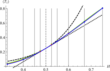
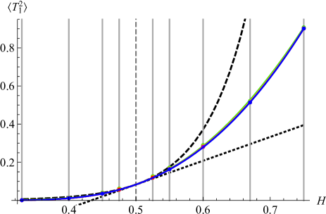
As usual, we have given two possible resummations. This will be tested later, see Fig. 19.

V Numerical validation

V.1 Algorithm

A numerical estimation of the calculated observables is obtained using the discrete-time algorithm by Davies and Harte DaviesHarte1987 , as described in DiekerPhD ; DiekerMandjes2003 . It generates for fBm of a given H𝐻H sample trajectories over a discretized time window [0,1]01[0,1]; the trajectories are drawn from a Gaussian probability with covariance (2). Time and space are then rescaled in respect of Eq. (2) s.t. not more than 104superscript10410^{-4} of all samples fail to exit for a given H𝐻H. (The time-scales in question are the upper times in the plots on Fig. 15.) While this induces a small systematic error, we can take advantage of the lin ×\times log performance of the Davies-Harte algorithm DaviesHarte1987 ; DiekerPhD ; DiekerMandjes2003 , whereas the execution time for a sequential generation of the sequence grows quadratically in time. Given the necessary system size, this would be very inefficient.
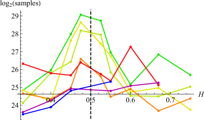
Refer to caption
Figure 9: Number of samples for each system size and value of H𝐻H. The color code is as in Fig. 10. Since the measured signal is proportional to ϵitalic-ϵ\epsilon, the error scales like the square root of the number of samples devided by |ϵ|italic-ϵ|\epsilon|. Thus more samples are needed for H𝐻H close to 1/2121/2, and only small systems can be simulated for H=0.475𝐻0.475H=0.475 and H=0.525𝐻0.525H=0.525.

V.2 Exit probability

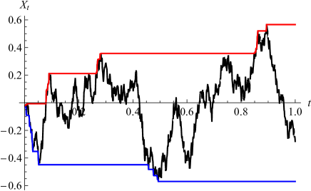
In order to measure P1(x)subscript𝑃1𝑥P_{1}(x) one could start the process Xtsubscript𝑋𝑡X_{t} at x𝑥x and measure whether Xtsubscript𝑋𝑡X_{t} is first absorbed at x=0𝑥0x=0 or x=1𝑥1x=1. This is very inefficient, as for each x𝑥x one has to run a simulation, and repeat the latter until the statistics is good enough. A slightly better strategy is to start with X0=0subscript𝑋00X_{0}=0, generate Xtsubscript𝑋𝑡X_{t}, shift it by x𝑥x, and check for each x𝑥x, whether it is first absorbed at x=0𝑥0x=0 or x=1𝑥1x=1. There is, however, a much more clever procedure, which we explain now, and which is illustrated on figure 12. Define for a random process Xtsubscript𝑋𝑡X_{t} the running max and min,

M+(t)subscript𝑀𝑡\displaystyle{M}_{+}(t) :=assign\displaystyle:= max0<t<tXt,subscript0superscript𝑡𝑡subscript𝑋superscript𝑡\displaystyle\max_{0<t^{\prime}<t}X_{t^{\prime}}\ , (110)
M(t)subscript𝑀𝑡\displaystyle{M}_{-}(t) :=assign\displaystyle:= min0<t<tXt.subscript0superscript𝑡𝑡subscript𝑋superscript𝑡\displaystyle\min_{0<t^{\prime}<t}X_{t^{\prime}}\ . (111)

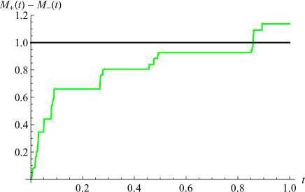
The total width or span s(t):=M+(t)M(t)assign𝑠𝑡subscript𝑀𝑡subscript𝑀𝑡s(t):={M}_{+}(t)-{M}_{-}(t) grows monotonically. We are interested in the time T1subscript𝑇1T_{1} when it attains 111. Define

T1subscript𝑇1\displaystyle T_{1} :=assign\displaystyle:= mint(M+(t)M(t)1),subscript𝑡subscript𝑀𝑡subscript𝑀𝑡1\displaystyle\min_{t}\big{(}{M}_{+}(t)-{M}_{-}(t)\geq 1\big{)}\ , (112)
x0subscript𝑥0\displaystyle x_{0} :=assign\displaystyle:= XT1XT1M+(T1)M(T1).subscript𝑋subscript𝑇1subscript𝑋subscript𝑇1subscript𝑀subscript𝑇1subscript𝑀subscript𝑇1\displaystyle X_{T_{1}}\equiv\frac{X_{T_{1}}}{{M}_{+}(T_{1})-{M}_{-}(T_{1})}\ . (113)

If the process starts for x>x0𝑥subscript𝑥0x>x_{0}, it will first be absorbed by the upper boundary (at x=1𝑥1x=1), whereas if it starts for x<x0𝑥subscript𝑥0x<x_{0}, it will first be absorbed by the lower one (at x=0𝑥0x=0). Denote the probability distribution of x0subscript𝑥0x_{0} by Px0(x)subscript𝑃subscript𝑥0𝑥P_{x_{0}}(x). It satisfies

Px0(x)=P0(x)=P1(x).subscript𝑃subscript𝑥0𝑥superscriptsubscript𝑃0𝑥superscriptsubscript𝑃1𝑥P_{x_{0}}(x)=-P_{0}^{\prime}(x)=P_{1}^{\prime}(x)\ . (114)

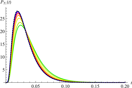
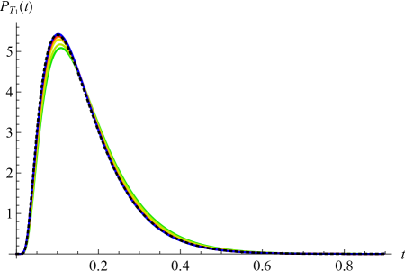
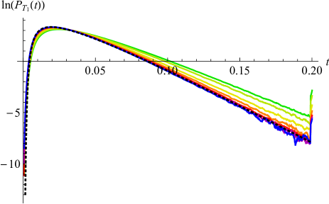
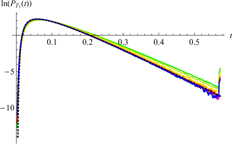
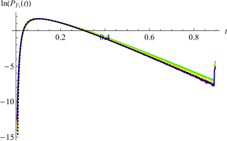
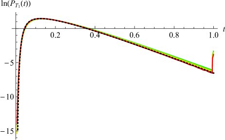
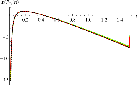
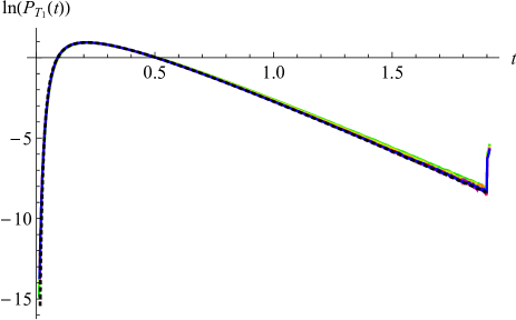
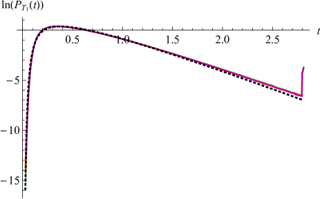
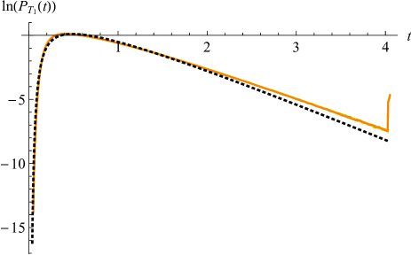
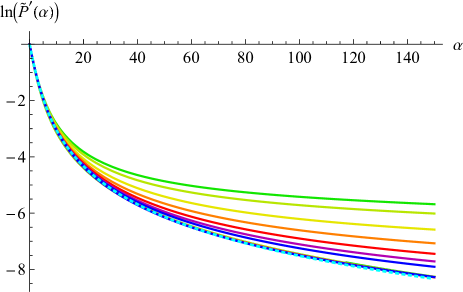
An example of the measurement of P1(x)superscriptsubscript𝑃1𝑥P_{1}^{\prime}(x) for H=0.33𝐻0.33H=0.33 is shown on figure 10. The most remarkable feature of this plot is the very slow convergence in system size towards the asymptotic curve, which via scaling is very close to a parabola, see Eqs. (70)–(71). This slow convergence can also be seen on the distribution PT1(t)subscript𝑃subscript𝑇1𝑡P_{T_{1}}(t) of the times T1subscript𝑇1T_{1} defined in Eq. (112). This is plotted on Fig. 15.
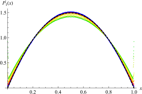
Refer to caption
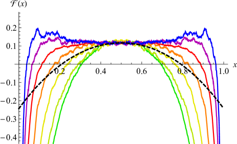
Figure 10: The measured probability P1(x)superscriptsubscript𝑃1𝑥P_{1}^{\prime}(x) for H=0.33𝐻0.33H=0.33. The system sizes are (from bottom to top at x=0.5𝑥0.5x=0.5): N=213𝑁superscript213N=2^{13} (dark green), 214superscript2142^{14} (green), 216superscript2162^{16} (olive), 218superscript2182^{18} (orange), 220superscript2202^{20} (red), 222superscript2222^{22} (dark magenta), 224superscript2242^{24} (blue). The dashed line is the scaling ansatz (70) (i.e. almost a parabola). Note the slow convergence for x0𝑥0x\to 0 and x1𝑥1x\to 1. Also note that the measured result for the largest system size at x=1/2𝑥12x=1/2 is larger than the scaling ansatz (70). This is equivalent to a positive curvature of the function (x)𝑥{\cal F}(x) defined in Eqs. (71) and (72), and given in the first (top left) plot of Fig. 13.

​​​(a)   Refer to caption             ​​​(b)Refer to caption

Figure 11: (a) The random process Xtsubscript𝑋𝑡X_{t}, with its running max (in red) and min (in blue), see main text. (b) The span, i.e. running max minus running min.

(a)  Refer to caption   ​​​​(b)  Refer to caption

Figure 12: (a) Mean (red) between the measured functions T(x)subscript𝑇𝑥{\cal F}_{T}(x) for H=0.45𝐻0.45H=0.45 (dark cyan, bottom line) and H=0.55𝐻0.55H=0.55 (dark green, top line). (b) ibid for T2(x)subscriptsuperscript𝑇2𝑥{\cal F}_{T^{2}}(x). System size used was N=224𝑁superscript224N=2^{24}, and the total number of samples is 1.64×1061.64superscript1061.64\times 10^{6} for H=0.45𝐻0.45H=0.45, and 2.19×1062.19superscript1062.19\times 10^{6} for H=0.55𝐻0.55H=0.55.

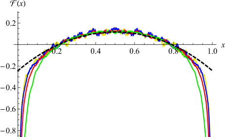
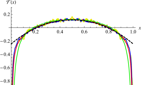
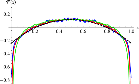
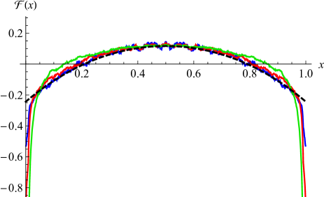
The slow convergence of P1(x)superscriptsubscript𝑃1𝑥P_{1}^{\prime}(x) can better be seen via the function (x)𝑥{\cal F}(x): An estimate of the latter can be extracted from the simulations, by inverting Eq. (71),

numϵ(x):=1ϵln(P(x)[x(1x)]21H)+const.assignsubscriptsuperscriptitalic-ϵnum𝑥1italic-ϵsuperscript𝑃𝑥superscriptdelimited-[]𝑥1𝑥21𝐻const{\cal F}^{\epsilon}_{\rm num}(x):=\frac{1}{\epsilon}\ln\left(P^{\prime}(x)[x(1-x)]^{2-\frac{1}{H}}\right)+\mbox{const}\ . (115)

The constant is chosen s.t. numϵ(1/2)=(1/2)subscriptsuperscriptitalic-ϵnum1212{\cal F}^{\epsilon}_{\rm num}(1/2)={\cal F}(1/2). According to our theory,

numϵ(x)=(x)+𝒪(ϵ).subscriptsuperscriptitalic-ϵnum𝑥𝑥𝒪italic-ϵ{\cal F}^{\epsilon}_{\rm num}(x)={\cal F}(x)+{\cal O}(\epsilon)\ . (116)

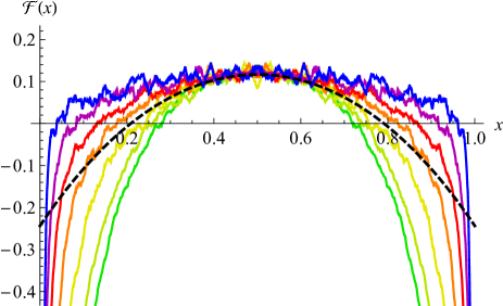
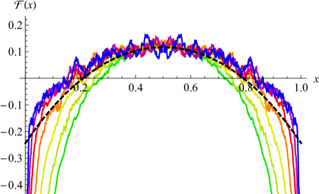
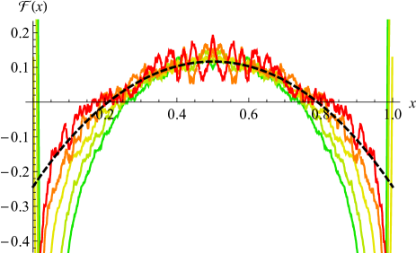
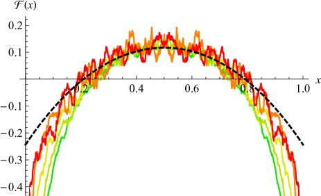
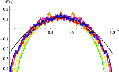
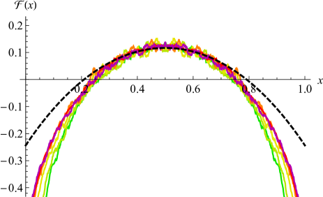
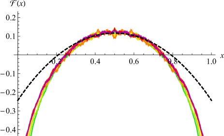
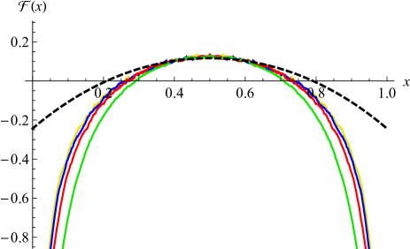
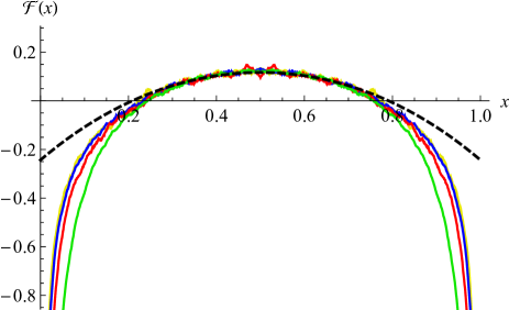
Examples are given on Fig. 13 (we suppressed all indices on {\cal F}). The case H=0.33𝐻0.33H=0.33 (upper left) corresponds to the plot on Fig. 10, with the same colors. One clearly sees that convergence in system size is slow for all H𝐻H, but especially for the smaller ones. It becomes better for larger values of H𝐻H.

Refer to caption
Refer to caption

H=0.33𝐻0.33H=0.33                                                                       H=0.4𝐻0.4H=0.4

Refer to caption
Refer to caption

H=0.45𝐻0.45H=0.45                                                                       H=0.475𝐻0.475H=0.475

Refer to caption
Refer to caption

H=0.525𝐻0.525H=0.525                                                                       H=0.55𝐻0.55H=0.55

Refer to caption
Refer to caption

H=0.6𝐻0.6H=0.6                                                                       H=0.67𝐻0.67H=0.67

Figure 13: The numerically estimated scaling function (x)𝑥{\cal F}(x) for (from top to bottom) N=213𝑁superscript213N=2^{13} (dark green), 214superscript2142^{14} (green), 216superscript2162^{16} (olive), 218superscript2182^{18} (orange), 220superscript2202^{20} (red), 222superscript2222^{22} (dark magenta), 224superscript2242^{24} (blue). The black dashed line is the result of Eq. (72). For ϵ=±0.025italic-ϵplus-or-minus0.025\epsilon=\pm 0.025, i.e. H=0.475𝐻0.475H=0.475 and H=0.525𝐻0.525H=0.525, due to the large statistics needed, we only simulated systems up to size N=220𝑁superscript220N=2^{20}. For H0.6𝐻0.6H\geq 0.6, convergence in system size is good, and we skipped the largest system N=224𝑁superscript224N=2^{24}. Note that the scaling ansatzof (70), i.e. 𝒫1,scaling(x)[x(1x)]1H2similar-tosuperscriptsubscript𝒫1scaling𝑥superscriptdelimited-[]𝑥1𝑥1𝐻2{\cal P}_{\rm 1,scaling}^{\prime}(x)\sim[x(1-x)]^{\frac{1}{H}-2} is equivalent to (x)0𝑥0{\cal F}(x)\equiv 0.
Refer to caption
Refer to caption

N=213𝑁superscript213N=2^{13}                                                                      N=216𝑁superscript216N=2^{16}

Refer to caption
Refer to caption

N=218𝑁superscript218N=2^{18}                                                                      N=220𝑁superscript220N=2^{20}

Refer to caption
Refer to caption

N=222𝑁superscript222N=2^{22}                                                                      N=224𝑁superscript224N=2^{24}

Refer to caption
Refer to caption
Figure 14: Dependence of the scaling function (x)𝑥{\cal F}(x) on N𝑁N, by taking the mean between H=1/2±ϵ𝐻plus-or-minus12italic-ϵH=1/2\pm\epsilon, for H=0.33/0.67𝐻0.330.67H=0.33/0.67 (green), H=0.4/0.6𝐻0.40.6H=0.4/0.6 (red), H=0.45/0.55𝐻0.450.55H=0.45/0.55 (blue), H=0.475/0.525𝐻0.4750.525H=0.475/0.525 (olive/yellow). For N=224𝑁superscript224N=2^{24}, we have replaced the estimate for H0.6𝐻0.6H\geq 0.6 by those of N=222𝑁superscript222N=2^{22}, justified by the much better convergence in system size for these values of H𝐻H, see figures 13. The last two plots show the extracted curvature γ𝛾\gamma with system sizes increasing from bottom to top: N=213𝑁superscript213N=2^{13} (green), N=214𝑁superscript214N=2^{14} (bright green), N=216𝑁superscript216N=2^{16} (olive/yellow), N=218𝑁superscript218N=2^{18} (orange), N=220𝑁superscript220N=2^{20} (red), N=222𝑁superscript222N=2^{22} (violet), N=224𝑁superscript224N=2^{24} (blue, single dot with big error bars). For the error estimate see Fig. 3. Note that the scaling ansatzof (70), i.e. 𝒫1,scaling(x)[x(1x)]1H2similar-tosuperscriptsubscript𝒫1scaling𝑥superscriptdelimited-[]𝑥1𝑥1𝐻2{\cal P}_{\rm 1,scaling}^{\prime}(x)\sim[x(1-x)]^{\frac{1}{H}-2} is equivalent to (x)0𝑥0{\cal F}(x)\equiv 0.

H=0.33𝐻0.33H=0.33                                                                       H=0.4𝐻0.4H=0.4

Refer to caption
Refer to caption

H=0.45𝐻0.45H=0.45                                                                       H=0.475𝐻0.475H=0.475

Refer to caption
Refer to caption

H=0.525𝐻0.525H=0.525                                                                       H=0.55𝐻0.55H=0.55

Refer to caption
Refer to caption

H=0.67𝐻0.67H=0.67                                                                       H=0.75𝐻0.75H=0.75

Refer to caption
Refer to caption
Figure 15: Probability distribution of the numerically estimated time T1subscript𝑇1T_{1} when the width of the process reaches 1, i.e. the process is absorbed irrespective of its starting position. N=213𝑁superscript213N=2^{13} (dark green), 214superscript2142^{14} (green), 216superscript2162^{16} (olive), 218superscript2182^{18} (orange), 220superscript2202^{20} (red), 222superscript2222^{22} (dark magenta), 224superscript2242^{24} (blue). The characteristic time depends quite strongly on H𝐻H. The result for H=1/2𝐻12H=1/2 is between the distributions for H=0.475𝐻0.475H=0.475, and H=0.525𝐻0.525H=0.525. The black dotted line is the analytic result for H=1/2𝐻12H=1/2, given in Eqs. (39)–(40), rescaled so that the first moment T1delimited-⟨⟩subscript𝑇1\left<T_{1}\right> is correctly reproduced. Small systematic deviations are visible for small and large values of H𝐻H, especially H=0.33𝐻0.33H=0.33, and H=0.75𝐻0.75H=0.75.

H=0.33𝐻0.33H=0.33                                                                       H=0.4𝐻0.4H=0.4

Refer to caption
Refer to caption

H=0.45𝐻0.45H=0.45                                                                       H=0.475𝐻0.475H=0.475

Refer to caption
Refer to caption

H=0.525𝐻0.525H=0.525                                                                       H=0.55𝐻0.55H=0.55

Refer to caption
Refer to caption

H=0.67𝐻0.67H=0.67                                                                       H=0.75𝐻0.75H=0.75

Refer to caption
Refer to caption
Figure 16: The same as figure 15, on a logarithmic scale. The little bump at large T𝑇T corresponds to all realizations which did not exit up to that time, i.e. it is the integrated tail.

We stopped our simulations after a total estimated 28 CPU years. It seems clear that measuring more than the curvature is illusory. We therefore defined

γ:=12x2numϵ(x)|x=1/2,assign𝛾evaluated-at12superscriptsubscript𝑥2superscriptsubscriptnumitalic-ϵ𝑥𝑥12\gamma:=\frac{1}{2}\partial_{x}^{2}{\cal F}_{\rm num}^{\epsilon}(x)\Big{|}_{x=1/2}\ , (117)

and in practice measured it by fitting a polynomial of degree two in an x𝑥x-range from x=0.25𝑥0.25x=0.25 to x=0.75𝑥0.75x=0.75 for the smaller systems, to x=0.15𝑥0.15x=0.15 to x=0.85𝑥0.85x=0.85 for the largest systems.

Analytically, we obtained in Eq. (74) with the Catalan constant C𝐶C,

γ=16(C1)=16n=1(1)n(2n+1)21.34455.𝛾16𝐶116superscriptsubscript𝑛1superscript1𝑛superscript2𝑛121.34455\gamma=16(C-1)=16\sum_{n=1}^{\infty}\frac{(-1)^{n}}{(2n+1)^{2}}\approx-1.34455\ . (118)

Our direct numerical estimate for γ𝛾\gamma is shown on Fig. 3. One sees that extrapolation to H=12𝐻12H=\frac{1}{2} is good only for large systems. An alternative and more precise way to extract γ𝛾\gamma is to define

¯numϵ(x):=12[numϵ(x)+numϵ(x)].assignsubscriptsuperscript¯italic-ϵnum𝑥12delimited-[]subscriptsuperscriptitalic-ϵnum𝑥subscriptsuperscriptitalic-ϵnum𝑥\overline{\cal F}^{\epsilon}_{\rm num}(x):=\frac{1}{2}\left[{\cal F}^{\epsilon}_{\rm num}(x)+{\cal F}^{-\epsilon}_{\rm num}(x)\right]\ . (119)

This combination cancels the first subleading contribution in ϵitalic-ϵ\epsilon; the result is plotted on Fig. 14. Again one sees that (x)𝑥{\cal F}(x) is well approximated for large system sizes. Our best estimate is

γnum=1.34±0.02.subscript𝛾numplus-or-minus1.340.02\gamma_{\rm num}=-1.34\pm 0.02\ . (120)

V.3 Expectation of exit times and their squares

​​​​(a)​​​​​​Refer to caption   (b)​​​​​​Refer to caption

Figure 17: (a) The mean, i.e. spatially averaged absorption time Tabs=01dxTabs(x)delimited-⟨⟩subscript𝑇abssuperscriptsubscript01differential-d𝑥delimited-⟨⟩subscript𝑇abs𝑥\left<T_{\rm abs}\right>=\int_{0}^{1}\mathrm{d}x\,\left<T_{\rm abs}(x)\right>. (b) ibid. for the second moment. The black dotted line is the direct expansion in ϵitalic-ϵ\epsilon, which underestimates the true result. The dashed line is the exponentiation of this correction; it overestimates the result. The fit to a quadratic polynomial is given in Eqs. (121) and (122).

Let us now turn to the exit times as a function of x𝑥x. Measurements of the scaling functions T(x)subscript𝑇𝑥{\cal F}_{T}(x) and T2(x)subscriptsuperscript𝑇2𝑥{\cal F}_{T^{2}}(x) given in Eqs. (IV.4) and (89)–(90) are presented on Fig. 12, for H=0.45𝐻0.45H=0.45 and H=0.55𝐻0.55H=0.55. Their mean (in red) is a good approximation of the analytic curves (in black dashed). Simulations were performed for the largest system size at our disposal N=224𝑁superscript224N=2^{24}, and H=0.45𝐻0.45H=0.45 as well as H=0.55𝐻0.55H=0.55. Having generated an fBm, we put its starting position at x𝑥x, and then searched for the first instance when it was absorbed at either the upper or lower boundary. This procedure turned out to be rather time-consuming, and we only evaluated this function about 2×1062superscript1062\times 10^{6} times.

To estimate the spatially averaged first two moments of the exit times, we fitted their numerically obtained values, supplemented with the analytically known values for H=1/2𝐻12H=1/2, with a polynomial of degree 2 in H𝐻H. The result, shown on Fig. 17 is

01dxTexit(x)=superscriptsubscript01differential-d𝑥delimited-⟨⟩subscript𝑇exit𝑥absent\displaystyle\!\!\!\int_{0}^{1}\mathrm{d}x\left<T_{\rm exit}(x)\right>= 112[1+8.73ϵ+19.1ϵ2+𝒪(ϵ3)],112delimited-[]18.73italic-ϵ19.1superscriptitalic-ϵ2𝒪superscriptitalic-ϵ3\displaystyle\frac{1}{12}\left[\textstyle 1+8.73\epsilon+19.1\epsilon^{2}+{\cal O}(\epsilon^{3})\right], (121)
01dxTexit2(x)=superscriptsubscript01differential-d𝑥delimited-⟨⟩superscriptsubscript𝑇exit2𝑥absent\displaystyle\!\!\!\int_{0}^{1}\mathrm{d}x\left<T_{\rm exit}^{2}(x)\right>= 160[1+17.1ϵ+100ϵ2+𝒪(ϵ3)].160delimited-[]117.1italic-ϵ100superscriptitalic-ϵ2𝒪superscriptitalic-ϵ3\displaystyle\frac{1}{60}\left[\textstyle 1+17.1\epsilon+100\epsilon^{2}+{\cal O}(\epsilon^{3})\right]. (122)

Comparison to Eqs. (95) and (103) yields excellent agreement for the first moment of the exit time (coefficient 8.7588.7588.758 to be compared to 8.738.738.73), and still very good agreement for the second moment (coefficient 16.56316.56316.563 as compared to 17.117.117.1). The latter is difficult to estimate, as higher-order corrections are seemingly large.

Let us finally mention that for H=1𝐻1H=1 the probability that starting at x𝑥x the exit time is t𝑡t, is given by

PexitH=1(t|x)=12πt2[xex22t2+(1x)e(1x)22t2].subscriptsuperscript𝑃𝐻1exitconditional𝑡𝑥12𝜋superscript𝑡2delimited-[]𝑥superscript𝑒superscript𝑥22superscript𝑡21𝑥superscript𝑒superscript1𝑥22superscript𝑡2P^{H=1}_{\rm exit}(t|x)=\frac{1}{\sqrt{2\pi}t^{2}}\left[xe^{-\frac{x^{2}}{2t^{2}}}+(1-x)e^{-\frac{(1-x)^{2}}{2t^{2}}}\right]\ . (123)

Averaging over x𝑥x yields

01dxPexitH=1(t|x)=2π[1e12t2].superscriptsubscript01differential-d𝑥subscriptsuperscript𝑃𝐻1exitconditional𝑡𝑥2𝜋delimited-[]1superscript𝑒12superscript𝑡2\int_{0}^{1}\mathrm{d}x\,P^{H=1}_{\rm exit}(t|x)=\sqrt{\frac{2}{\pi}}\left[1-e^{-\frac{1}{2t^{2}}}\right]\ . (124)

All these distributions at H=1𝐻1H=1 are patologic. While they are normalizable, they have large tails which render already the first moment undefined. They are thus not a useful limit to test our formulas.

V.4 The time the span reaches 1

Our algorithm presented in section V.1 to determine P1(x)subscriptsuperscript𝑃1𝑥P^{\prime}_{1}(x) first determines the time the span (running max minus running min) reaches 1. For Brownian motion, its probability distribution was given in Eqs. (39) and (40). As we have seen in section IV.9, it gets corrected for H1/2𝐻12H\neq 1/2, in a way we are currently unable to obtain analytically. The question we ask is how much does it differ from the result for Brownian motion? The most important effect is a change in time scale, which we estimated in Eq. (108). Our numerical estimates, shown on Fig. 19 lead to

T1delimited-⟨⟩subscript𝑇1\displaystyle\left<T_{1}\right> =\displaystyle= 14[1+7.4ϵ+10.1ϵ218ϵ3+],14delimited-[]17.4italic-ϵ10.1superscriptitalic-ϵ218superscriptitalic-ϵ3\displaystyle\frac{1}{4}\left[1+7.4\epsilon+10.1\epsilon^{2}-18\epsilon^{3}+...\right]\ , (125)
T12delimited-⟨⟩superscriptsubscript𝑇12\displaystyle\left<T_{1}^{2}\right> =\displaystyle= 112[1+15ϵ+75ϵ2+110ϵ3+].112delimited-[]115italic-ϵ75superscriptitalic-ϵ2110superscriptitalic-ϵ3\displaystyle\frac{1}{12}\left[1+15\epsilon+75\epsilon^{2}+110\epsilon^{3}+...\right]\ .\qquad (126)

This is in good agreement with Eqs. (108)-(109), where the order-ϵitalic-ϵ\epsilon coefficients read 7.457.457.45 and 14.9614.9614.96, respectively.

In order to compare the full distributions, we superimposed on the measured distribution the result for Brownian motion, rescaled s.t. the first moment T1delimited-⟨⟩subscript𝑇1\left<T_{1}\right> is correctly reproduced. The result of this procedure is shown on figures 15 and 16. One can see deviations for large |ϵ|italic-ϵ|\epsilon|, especially H=0.75𝐻0.75H=0.75, which on the whole rest surprisingly small.

Finally, it is easy to show analytically that for H=1𝐻1H=1,

PT1H=1(t)=2πe12t2t2.superscriptsubscript𝑃subscript𝑇1𝐻1𝑡2𝜋superscript𝑒12superscript𝑡2superscript𝑡2P_{T_{1}}^{H=1}(t)=\sqrt{\frac{2}{\pi}}\frac{e^{-\frac{1}{2t^{2}}}}{t^{2}}\ . (127)

As the distributions (123) and (124), Eq. (127) has a large tail, leading to undefined moments.

V.5 Finite-discretization effects

As we saw on Fig. 10, there are important finite-discretization corrections. This is even more visible on Fig. 13, especially for H=0.33𝐻0.33H=0.33 (upper left corner). To better understand where this comes from, consider Fig. 12. In the given example, the width 111 is reached at T10.85subscript𝑇10.85T_{1}\approx 0.85, with x00.58subscript𝑥00.58x_{0}\approx 0.58. What is the error made, due to the finite discretization in time? Our argument will be made, as in the drawing, for a particle trajectory “exiting at the upper boundary”, i.e. at tsubscript𝑡t_{*} the running max M+(t)subscript𝑀𝑡M_{+}(t) is growing, whereas the running min M(t)subscript𝑀𝑡M_{-}(t) is constant.

Refer to caption
Figure 18: Top 7 curves: The logarithm of P~(α)superscript~𝑃𝛼\tilde{P}^{\prime}(\alpha) (Laplace transform of P(x)superscript𝑃𝑥P^{\prime}(x), as plotted on Fig. 10), for system sizes N=213𝑁superscript213N=2^{13} (top, green) to N=224𝑁superscript224N=2^{24} (blue). The lower solid curve are a scaling collapse of all 7 curves, using Eqs. (132) and (133). The blue dashed line is the Laplace transform of the scaling ansatz (70), plotted on Fig. 10.

The error in estimating the max is without consequences: while the true running max could be underestimated, this would only result in a slight underestimation of tsubscript𝑡t_{*}. The problem in estimating M(t)subscript𝑀𝑡M_{-}(t) is more severe: if we underestimate the true minimum by δ𝛿\delta, then x0subscript𝑥0x_{0} is

x0=M(t)+δ.subscript𝑥0subscript𝑀𝑡𝛿x_{0}=M_{-}(t)+\delta\ . (128)

Denote PNmiss(δ)superscriptsubscript𝑃𝑁miss𝛿P_{N}^{\rm miss}(\delta) the distribution of δ𝛿\delta. Close to the lower boundary, the probability at system size N𝑁N, PN(x)subscriptsuperscript𝑃𝑁𝑥P^{\prime}_{N}(x), is

PN(x)=0dδPNmiss(δ)PN=(xδ).subscriptsuperscript𝑃N𝑥superscriptsubscript0differential-d𝛿superscriptsubscript𝑃𝑁miss𝛿subscriptsuperscript𝑃𝑁𝑥𝛿P^{\prime}_{\rm N}(x)=\int_{0}^{\infty}\mathrm{d}\delta\,P_{N}^{\rm miss}(\delta)P^{\prime}_{N=\infty}(x-\delta)\ . (129)

The function PNmiss(δ)superscriptsubscript𝑃𝑁miss𝛿P_{N}^{\rm miss}(\delta) should be a function of δ/τH𝛿superscript𝜏𝐻\delta/\tau^{H}, where τ=1/N𝜏1𝑁\tau=1/N, thus

PNmiss(δ)=Pmiss(δNH).superscriptsubscript𝑃𝑁miss𝛿superscript𝑃miss𝛿superscript𝑁𝐻P_{N}^{\rm miss}(\delta)=P^{\rm miss}\left(\delta N^{H}\right)\ . (130)

Transforming to Laplace variables, Eq. (129) reads (with the tilde indicating the Laplace transform)

P~N(α)=P~N=(α)P~miss(α/NH).subscriptsuperscript~𝑃𝑁𝛼subscriptsuperscript~𝑃𝑁𝛼superscript~𝑃miss𝛼superscript𝑁𝐻\tilde{P}^{\prime}_{N}(\alpha)=\tilde{P}^{\prime}_{N=\infty}(\alpha)\tilde{P}^{\rm miss}(\alpha/N^{H})\ . (131)

Taking a log and rearranging yields

ln(P~N=(α))=ln(P~N(α))ln(P~miss(α/NH)).subscriptsuperscript~𝑃𝑁𝛼subscriptsuperscript~𝑃𝑁𝛼superscript~𝑃miss𝛼superscript𝑁𝐻\ln\left(\tilde{P}^{\prime}_{N=\infty}(\alpha)\right)=\ln\left(\tilde{P}^{\prime}_{N}(\alpha)\right)-\ln\left(\tilde{P}^{\rm miss}(\alpha/N^{H})\right)\ . (132)

​​​​​​​​(a)​​​ Refer to caption        ​​​​(b)​​​​​​Refer to caption

Figure 19: Left: The expectation T1delimited-⟨⟩subscript𝑇1\left<T_{1}\right>. The data-points with interpolation follow the color code of Fig. 15. The black dotted line from Eq. (108) is the direct expansion in ϵitalic-ϵ\epsilon, which underestimates the numerical result, while its exponentiation given by the dashed line overestimates it. Right: ibid. for T12delimited-⟨⟩superscriptsubscript𝑇12\left<T_{1}^{2}\right>, with the analytical result given in Eq. (109).

We currently have no theory for P~miss(α)subscript~𝑃miss𝛼\tilde{P}_{\rm miss}(\alpha), but we find that a decent approximation for H=0.33𝐻0.33H=0.33 is given by

ln(P~miss(α))0.38ln(P~bridge(1.7α)).subscript~𝑃miss𝛼0.38subscript~𝑃bridge1.7𝛼\ln\left(\tilde{P}_{\rm miss}(\alpha)\right)\approx 0.38\ln\left(\tilde{P}_{\rm bridge}(1.7\alpha)\right)\ . (133)

The function Pbridge(m)subscript𝑃bridge𝑚P_{\rm bridge}(m) is the maximum of a fBm bridge for duration T=1𝑇1T=1, as given in Eq. (90) of Ref. DelormeWiese2016b . Note that the numerical values of 0.380.380.38 and 1.71.71.7 are not significant. (Increasing one will decrease the other). As stated above, this formula is a guess, based on the following observations and hypothesis: Suppose that we measured a maximum m𝑚m at time t𝑡t, that the true maximum is between times t𝑡t and t+1/N𝑡1𝑁t+1/N, and that at time t+1/N𝑡1𝑁t+1/N the process again achieves its maximum (it should be smaller than the maximum), then for Brownian motion the probability for the true maximum will be given by (133) with the numerical values put to 1. For a fBm, we again use the bridge process with the appropriate H𝐻H. As for H1/2𝐻12H\neq 1/2 the process is correlated, our ansatz induces a new error as it neglects correlations with the positions of the other points. The numbers induced above seem to compensate for the approximations made.

These arguments are illustrated on Fig. 18. The top seven curves show ln(P~N(α))subscriptsuperscript~𝑃𝑁𝛼\ln\!\big{(}\tilde{P}^{\prime}_{N}(\alpha)\big{)} for system sizes N=213𝑁superscript213N=2^{13} (green, top), to N=224𝑁superscript224N=2^{24} (blue, second last curve from the bottom). The remaining lower curve is a scaling collapse estimating ln(P~N=(α))subscriptsuperscript~𝑃𝑁𝛼\ln\big{(}\tilde{P}^{\prime}_{N=\infty}(\alpha)\big{)}, with Pmiss(α)subscript𝑃miss𝛼P_{\rm miss}(\alpha) given in Eq. (133). The dashed line (cyan) is the Laplace transform of the scaling ansatz (70).

Our analysis shows that (i) discretization corrections are important, (ii) they come from an underestimation of the extension of the process on the side at which it does not exit, (iii) there exists a correcting function one should be able to calculate analytically. The latter task is left for future research.

VI Conclusion

In this article, we considered the two-sided exit problem from a strip. We gave analytic results for the exit probabilities and times, in an expansion in H1/2𝐻12H-1/2. While our numerical simulations confirm our findings, they also point to a fundamental problem: If the observation of the underlying process is not done continuously but at a finite number of equally spaced times, the situation is exactly as in our numerical simulations. As a consequence, one may not see the predicted analytic form, and not even the correct scaling laws. It will be important to quantify these effects to properly interpret experimental data once they appear.

We also considered the probability distribution for the time the span (running max minus running mean), i.e. the area the process has visited, reaches 1. We gave analytic expressions of this probability for Brownian motion, seemingly absent from the literature. For an fBM, evaluating corrections to its first moment analytically allows us to give a rather good approximation for this observable, without any adjustable parameter.

Our results can be extended to include drift, and to one or two reflecting boundaries.


ACKNOWLEDGMENTS


It is a pleasure to thank Olivier Benichou, Mathieu Delorme, Alberto Rosso, Alejandro Kolton, Tridib Sadhu and Sidney Redner for stimulating discussions, and the two referees for their constructive remarks.

References