Neutrino emission from the direction of the blazar TXS 0506+056 prior to the IceCube-170922A alert

A high-energy neutrino event detected by IceCube on 22 September 2017 was coincident in direction and time with a gamma-ray flare from the blazar TXS 0506+056. Prompted by this association, we investigated 9.5 years of IceCube neutrino observations to search for excess emission at the position of the blazar. We found an excess of high-energy neutrino events with respect to atmospheric backgrounds at that position between September 2014 and March 2015. Allowing for time-variable flux, this constitutes ${3.5\sigma}$ evidence for neutrino emission from the direction of TXS 0506+056, independent of and prior to the 2017 flaring episode. This suggests that blazars are the first identifiable sources of the high-energy astrophysical neutrino flux.

The origin of the highest-energy cosmic rays is believed to be extragalactic  (?), but their acceleration sites remain unidentified. High-energy neutrinos are expected to be produced in or near the acceleration sites when cosmic rays interact with matter and ambient light, producing charged mesons that decay into neutrinos and other particles. Unlike cosmic rays, neutrinos can travel through the Universe unimpeded by interactions with other particles and undeflected by magnetic fields, providing a means to identify and study the extreme environments producing cosmic rays  (?). Blazars, a class of active galactic nuclei with powerful relativistic jets pointed close to our line of sight  (?), are prominent candidate sources of such high-energy neutrino emission  (?, ?, ?, ?, ?, ?). The electromagnetic emission of blazars is observed to be highly variable on time-scales from minutes to years  (?).

The IceCube Neutrino Observatory  (?) is a high-energy neutrino detector occupying an instrumented volume of 1 km³ within the Antarctic ice sheet at the Amundsen-Scott South Pole Station. The detector consists of an array of 86 vertical strings, nominally spaced 125 m apart and descending to a depth of approximately 2450 m in the ice. The bottom 1 km of each string is equipped with 60 optical sensors that record Cherenkov light emitted by relativistic charged particles passing through the optically transparent ice. When high-energy muon neutrinos interact with the ice, they can create relativistic muons that travel many kilometers, creating a track-like series of Cherenkov photons recorded when they pass through the array. This allows the reconstruction of the original neutrino direction with a median angular uncertainty of $0.5^{\circ}$ for a neutrino energy of $\sim 30$ TeV (or $0.3^{\circ}$ at 1 PeV)  (?, ?).

IceCube discovered the existence of a diffuse flux of high-energy astrophysical neutrinos in 2013  (?, ?). Measurements of the energy spectrum have since been refined  (?, ?), indicating that the neutrino spectrum extends above several PeV. However, analyses of neutrino observations have not succeeded in identifying individual sources of high-energy neutrinos  (?, ?). This suggests that the sources are distributed across the sky and that even the brightest individual sources contribute only a small fraction of the total observed flux.

Recently, the detection of a high-energy neutrino by IceCube, together with observations in gamma rays and at other wavelengths, indicates that a blazar, TXS 0506+056, located at right ascension (RA) $77.3582^{\circ}$ and declination (Dec) $+5.69314^{\circ}$ (J2000 equinox)  (?) may be an individually identifiable source of high-energy neutrinos (?). The neutrino-candidate event, IceCube-170922A, was detected on 22 September 2017, selected by the Extremely High Energy (EHE) online event filter  (?), and reported as a public alert  (?). EHE alerts are currently sent at a rate of about four per year, and are based on well-reconstructed, high-energy muon-track events. The selection threshold is set so that approximately half of the events are estimated to be astrophysical neutrinos, the rest being atmospheric background events. After the alert was sent, further studies refined the directional reconstruction, with best-fitting coordinates of RA 77.43${}_{-0.65}^{+0.95}$ and Dec $+5.72_{-0.30}^{+0.50}$ (deg, J2000, 90% containment region). The most probable neutrino energy was estimated to be 290 TeV, with a 90% confidence level lower limit of 183 TeV  (?).

It was soon determined that the direction of IceCube-170922A was consistent with the location of TXS 0506+056 and coincident with a state of enhanced gamma-ray activity observed since April 2017  (?) by the Large Area Telescope (LAT) on the Fermi Gamma-ray Space Telescope (?). Follow-up observations of the blazar led to the detection of gamma rays with energies up to 400 GeV by the Major Atmospheric Gamma Imaging Cherenkov (MAGIC) Telescopes  (?, ?). IceCube-170922A and the electromagnetic observations are described in detail in  (?). The significance of the spatial and temporal coincidence of the high-energy neutrino and the blazar flare is estimated to be at the $3\sigma$ level  (?). On the basis of this result, we consider the hypothesis that the blazar TXS 0506+056 has been a source of high-energy neutrinos beyond that single event.

Searching for neutrino emission

IceCube monitors the whole sky and has maintained essentially continuous observations since 5 April 2008. Searches for neutrino point sources using two model-independent methods, a time-integrated and a time-dependent unbinned maximum likelihood analysis, have previously been published for the data collected between 2008 and 2015  (?, ?, ?). Here, we analyze the same 7-year data sample supplemented with additional data collected from May 2015 until October 2017  (?). The data span 9.5 years and consist of six distinct periods, corresponding to changing detector configurations, data-taking conditions, and improved event selections (Table 1).

Sample	Start	End
IC40	2008 Apr     5	2009 May 20
IC59	2009 May 20	2010 May 31
IC79	2010 May 31	2011 May 13
IC86a	2011 May 13	2012 May 16
IC86b	2012 May 16	2015 May 18
IC86c	2015 May 18	2017  Oct  31

Table 1: IceCube neutrino data samples. Six data-taking periods make up the full 9.5-year data sample. Sample numbers correspond to the number of detector strings that were operational. During the first three periods, the detector was still under construction. The last three periods correspond to different data-taking conditions and/or event selections with the full 86-string detector.

The northern sky, where TXS 0506+056 is located, is observed through Earth by IceCube. Approximately 70,000 neutrino-induced muon tracks are recorded each year from this hemisphere of the sky after passing the final event selection criteria. Fewer than 1% of these events originate from astrophysical neutrinos; the vast majority are background events caused by neutrinos of median energy $\sim 1$ TeV created in cosmic-ray interactions in the atmosphere over other locations on Earth. However, for an astrophysical muon-neutrino flux where the differential number of neutrinos with energy $E$ scales like $dN/dE\sim E^{-2}$, the distribution of muon energies is different than for the background atmospheric neutrino flux, which scales as $\sim E^{-3.7}$  (?). This allows for further discriminating power in point source searches besides directional-only excesses.

A high-significance point-source detection  (?, ?) can require between as few as two or three, or as many as 30, signal events to stand out from the background, depending on the energy spectrum and the clustering of events in time. To search for a neutrino signal at the coordinates of TXS 0506+056, we apply the standard time-integrated analysis  (?) and time-dependent analysis  (?) that have been used in past searches  (?, ?, ?). The time-integrated analysis uses an unbinned maximum-likelihood ratio method to search for an excess number of events consistent with a point source at a specified location, given the angular distance and angular uncertainty of each event. Energy information is included in the definition of the likelihood, assuming a power-law energy spectrum, $E^{-\gamma}$, with the spectral index $\gamma$ as a fitted parameter. The model parameters are correlated and are expressed as a pair, ($\Phi_{100}$, $\gamma$), where $\Phi_{100}$ is the flux normalization at 100 TeV. The time-dependent analysis uses the same formulation of the likelihood but searches for clustering in time as well as space by introducing an additional time profile. It is performed separately for two different generic profile shapes: a Gaussian-shaped time window and a box-shaped time window. Each analysis varies the central time of the window, $T_{0}$, and the duration $T_{\mathrm{W}}$ (from seconds to years) of the potential signal to find the four parameters $(\Phi_{100},\gamma,T_{0},T_{\mathrm{W}})$ that maximize the likelihood ratio, which is defined as the test statistic $TS$. (For the Gaussian time window, $T_{\mathrm{W}}$ represents twice the standard deviation.) The test statistic includes a factor that corrects for the look-elsewhere effect arising from all of the possible time windows that could be chosen  (?).

For each analysis method (time-integrated and time-dependent), a robust significance estimate is obtained by performing the identical analysis on trials with randomized data sets. These are produced by randomizing the event times and re-calculating the RA coordinates within each data-taking period. The resultant $P$ value is defined as the fraction of randomized trials yielding a value of $TS$ greater than or equal to the one obtained for the actual data.

Because the detector configuration and event selections changed as shown in Table 1, the time-dependent analysis is performed by operating on each data-taking period separately. (A flare that spans a boundary between two periods could be partially detected in either period, but with reduced significance.) An additional look-elsewhere correction then needs to be applied for a result in an individual data segment, given by the ratio of the total 9.5 year observation time to the observation time of that data segment  (?).

Neutrinos from the direction of TXS 0506+056

The results of the time-dependent analysis performed at the coordinates of TXS 0506+056 are shown in Fig. 1 for each of the six data periods. One of the data periods, IC86b from 2012 to 2015, contains a significant excess which is identified by both time-window shapes. The excess consists of $13\pm 5$ events above the expectation from the atmospheric background. The significance depends on the energies of the events, their proximity to the coordinates of TXS 0506+056, and their clustering in time. This is illustrated in Fig. 2, which shows the time-independent weight of individual events in the likelihood analysis during the IC86b data period.

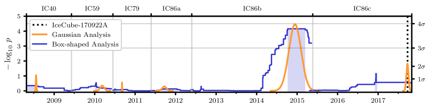
Figure 1: Time-dependent analysis results. The orange curve corresponds to the analysis using the Gaussian-shaped time profile. The central time $T_{0}$ and width $T_{\mathrm{W}}$ are plotted for the most significant excess found in each period, with the $P$ value of that result indicated by the height of the peak. The blue curve corresponds to the analysis using the box-shaped time profile. The curve traces the outer edge of the superposition of the best-fitting time windows (durations $T_{\mathrm{W}}$) over all times $T_{0}$, with the height indicating the significance of that window. In each period, the most significant time window forms a plateau, shaded in blue. The large blue band centered near 2015 represents the best-fitting 158-day time window found using the box-shaped time profile. The vertical dotted line in IC86c indicates the time of the IceCube-170922A event.

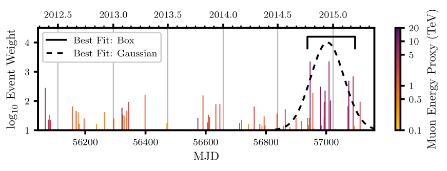
Figure 2: Time-independent weight of individual events during the IC86b period. Each vertical line represents an event observed at the time indicated by calendar year (top) or MJD (bottom). Overlapping lines are shifted by 1 to 2 days for visibility. The height of each line indicates the Event Weight: the product of the event’s spatial term and energy term in the unbinned likelihood analysis evaluated at the location of TXS 0506+056 and assuming the best-fitting spectral index $\gamma=2.1$  (?). The color for each event indicates an approximate value in units of TeV of the reconstructed muon energy (Muon Energy Proxy), which the analysis compares with expected muon energy distributions under different hypotheses. [A distribution for the true neutrino energy of a single event can also be inferred from the event’s muon energy, see  (?)]. The dashed curve and the solid bracket indicate the best-fitting Gaussian and box-shaped time windows, respectively. The distribution of event weights and times outside of the best-fitting time windows is compatible with background.

The Gaussian time window is centered at 13 December 2014 [modified Julian day (MJD) 57004] with an uncertainty of $\pm 21$ days and a duration $T_{\mathrm{W}}=110_{-24}^{+35}$ days. The best-fitting parameters for the fluence $J_{100}=\int\Phi_{100}(t)dt$ and the spectral index are given by $E^{2}J_{100}=(2.1^{+0.9}_{-0.7})\times 10^{-4}$ TeV cm^-2 at 100 TeV and $\gamma=2.1\pm 0.2$, respectively. The joint uncertainty on these parameters is shown in Fig. 3 along with a skymap showing the result of the time-dependent analysis performed at the location of TXS 0506+056 and in its vicinity during the IC86b data period.

The box-shaped time window is centered 13 days later with duration $T_{\mathrm{W}}=158$ days (from MJD 56937.81 to MJD 57096.21, inclusive of contributing events at boundary times). For the box-shaped time window the uncertainties are discontinuous and not well-defined, but the uncertainties for the Gaussian window show that it is consistent with the box-shaped time window fit. Despite the different window shapes, which lead to different weightings of the events as a function of time, both windows identify the same time interval as significant. For the box-shaped time window, the best-fitting parameters are similar to those of the Gaussian window, with fluence at 100 TeV and spectral index given by $E^{2}J_{100}=(2.2^{+1.0}_{-0.8})\times 10^{-4}$ TeV cm^-2 and $\gamma=2.2\pm 0.2$. This fluence corresponds to an average flux over 158 days of $\Phi_{100}=(1.6^{+0.7}_{-0.6})\times 10^{-15}$ TeV^-1 cm^-2 s^-1.

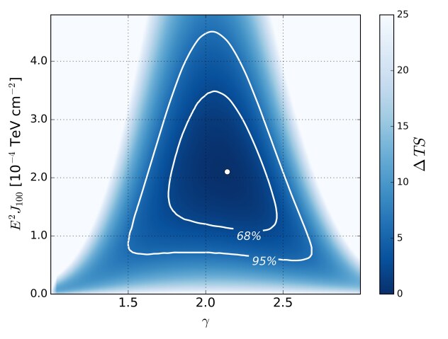
(a)

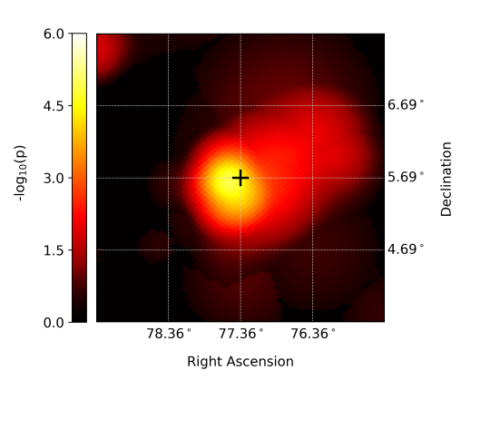
(b)

Figure 3: Time-dependent analysis results for the IC86b data period (2012-2015). (a) Change in test statistic, $\Delta TS$, as a function of the spectral index parameter $\gamma$ and the fluence at 100 TeV given by $E^{2}J_{100}$. The analysis is performed at the coordinates of TXS 0506+056, using the Gaussian-shaped time window and holding the time parameters fixed ($T_{0}=$ 13 December 2014, $T_{\mathrm{W}}=110$ days). The white dot indicates the best-fitting values. The contours at 68% and 95% confidence level assuming Wilks’ theorem  (?) are shown in order to indicate the statistical uncertainty on the parameter estimates. Systematic uncertainties are not included. (b) Skymap showing the $P$ value of the time-dependent analysis performed at the coordinates of TXS 0506+056 (cross) and at surrounding locations. The analysis is performed on the IC86b data period, using the Gaussian-shaped time-window. At each point, the full fit for $(\Phi,\gamma,T_{0},T_{\mathrm{W}})$ is performed. The $P$ value shown does not include the look-elsewhere effect related to other data periods. An excess of events is detected consistent with the position of TXS 0506+056.

When we estimate the significance of the time-dependent result by performing the analysis at the coordinates of TXS 0506+056 on randomized data sets, we allow in each trial a new fit for all the parameters: $\Phi_{100},\gamma,T_{0},T_{\mathrm{W}}$. We find that the fraction of randomized trials that result in a more significant excess than the real data is $7\times 10^{-5}$ for the box-shaped time window and $3\times 10^{-5}$ for the Gaussian time window. This fraction, once corrected for the ratio of the total observation time to the IC86b observation time (9.5 years / 3 years), results in $P$ values of $2\times 10^{-4}$ and $10^{-4}$, respectively, corresponding to $3.5\sigma$ and $3.7\sigma$. Because there is no a priori reason to prefer one of the generic time-windows over the other, we take the more significant one and include a trial factor of 2 for the final significance, which is then $3.5\sigma$.

Outside the 2012-2015 time period, the next most significant excess is found using the Gaussian window in 2017 and includes the IceCube-170922A event. This time window is centered at 22 September 2017 with duration $T_{\mathrm{W}}=19$ days, $\gamma=1.7\pm 0.6$, and fluence $E^{2}J_{100}=0.2_{-0.2}^{+0.4}\times 10^{-4}$ TeV cm^-2 at 100 TeV. No other event besides the IceCube-170922A event contributes significantly to the best-fit. As a consequence, the uncertainty on the best-fitting window location and width spans the entire IC86c period, because any window containing IceCube-170922A yields a similar value of the test statistic. Following the trial-correction procedure for different observation periods as described above, the significance of this excess is $1.4\sigma$. If the IceCube-170922A event is removed, no excess remains during this time period. This agrees with the result of the rapid-response analysis  (?) that is part of the IceCube alert program, which found no other potential astrophysical neutrinos from the same region of the sky during $\pm 7$ days centered on the time of IceCube-170922A.

We performed a time-integrated analysis at the coordinates of TXS 0506+056 using the full 9.5 year-data sample. The best-fitting parameters for the flux normalization and the spectral index are $\Phi_{100}=$ $(0.8^{+0.5}_{-0.4})\times 10^{-16}$ TeV^-1 cm^-2 s^-1 and $\gamma=2.0\pm 0.3$, respectively. The joint uncertainty on these parameters is shown in Fig. 4a. The $P$ value, based on repeating the analysis at the same coordinates with randomized data sets, is 0.002% ($4.1\sigma$), but this is an a posteriori significance estimate because it includes the IceCube-170922A event which motivated performing the analysis at the coordinates of TXS 0506+056. An unbiased significance estimate including the event would need to take into account the look-elsewhere effect related to all other possible directions in the sky that could be analyzed. It is expected that there will be two or three directions somewhere in the northern sky with this significance or greater resulting from the chance alignment of neutrinos  (?). Here we are interested in determining whether there is evidence of time-integrated neutrino emission from TXS 0506+056 besides the IceCube-170922A event.

If we remove the final data period IC86c, which contains the event, and perform the analysis again using only the first 7 years of data, we find best-fitting parameters that are nearly unchanged: $\Phi_{100}=(0.9^{+0.6}_{-0.5})\times 10^{-16}$ TeV^-1 cm^-2 s^-1 and $\gamma=2.1\pm 0.3$, respectively. The joint uncertainty on these parameters is shown in Fig. 4b. The $P$ value, using only the first 7 years of data, is 1.6% ($2.1\sigma$), based on repeating the analysis at the same coordinates with randomized data sets. These results indicate that the time-integrated fit is dominated by the same excess as found in the time-dependent analysis above, having similar values for the spectral index and total fluence ($E^{2}J_{100}=2.0\times 10^{-4}$ TeV cm^-2 at 100 TeV, over the 7-year period). This excess is not significant in the time-integrated analysis because of the additional background during the rest of the 7-year period.

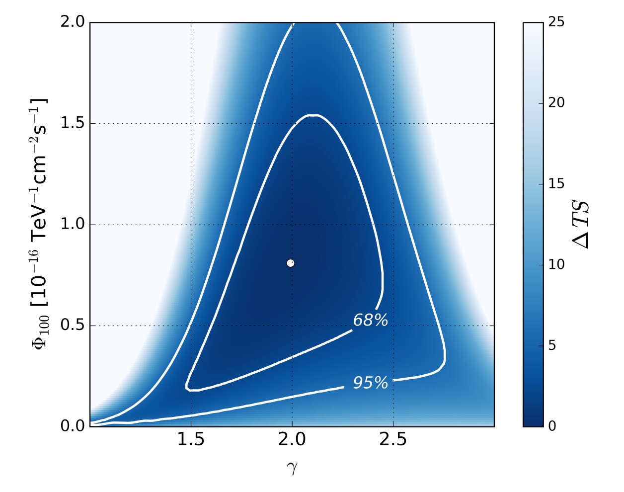
(a)

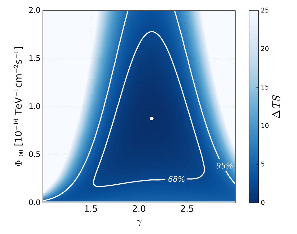
(b)

Figure 4: Time-integrated analysis results. As in Fig. 3a, but for the time-integrated analysis of TXS 0506+056 using (a) the full 9.5 year sample (2008-2017), and (b) the 7 year sample (2008-2015).

Blazars as neutrino sources

The signal identified during the 5-month period in 2014-2015 consists of an estimated $13\pm 5$ muon-neutrino events that are present in addition to the expected background. The analysis is unbinned, but the mean background at the declination of TXS 0506+056 is useful for comparison purposes; it is 5.8 events in a search bin of radius $1^{\circ}$ during a 158-day time window. (We use the duration of the box-shaped time-window result for convenience to calculate averages during the flare.) The significance of the excess is due to both the number of events and their energy distribution, with higher-energy events increasing the significance and leading to the best-fitting spectral-index of 2.1, in contrast to the lower energy atmospheric neutrino background with spectral index $\sim 3.7$. At this declination in the sky, the 68% central energy range in which IceCube is most sensitive to point sources with $E^{-2.1}$ spectra is between 32 TeV and 3.6 PeV. Assuming that the muon-neutrino fluence ($E^{2}J_{100}=(2.1^{+1.0}_{-0.7})\times 10^{-4}$ TeV cm^-2) is one-third of the total neutrino fluence, then the all-flavor neutrino energy fluence is $(4.2^{+2.0}_{-1.4})\times 10^{-3}$ erg cm^-2 over this energy range. With the recent measurement  (?) of the redshift of TXS 0506+056 as $z=0.3365\pm 0.0010$, this energy fluence implies that the isotropic neutrino luminosity is $(1.2^{+0.6}_{-0.4})\times 10^{47}$ erg s^-1 averaged over 158 days. This is higher than the isotropic gamma-ray luminosity during the same period, which is similar to the long-term luminosity between 0.1 GeV and 100 GeV of $0.28\times 10^{47}$ erg s^-1 averaged over all Fermi-LAT observations of TXS 0506+056  (?). Gamma rays are expected to be produced in the same processes that produce neutrinos—for example, when accelerated protons interact with ambient lower-energy photons near the source, producing both neutral pions (which decay to gamma-rays) and charged pions (which decay to neutrinos and leptons). A higher luminosity in neutrinos than in gamma rays could imply that a substantial fraction of the gamma rays related to the neutrino production are either absorbed or arriving at energies above or below the Fermi-LAT energy band.

Although TXS 0506+056 is a bright object in gamma rays, it was not previously singled out as a predicted neutrino source. In the third catalog of active galactic nuclei detected by Fermi-LAT  (?) listing 1773 objects (including those at low galactic latitudes), TXS 0506+056 is among the 50 brightest objects, with an average flux between 1 GeV and 100 GeV of ($6.5\pm 0.2)\times 10^{-9}$ photons cm^-2 s^-1. Its measured redshift now makes it one of the most luminous objects known out to the same distance, more than an order of magnitude more luminous than nearby blazars such as Markarian 421, Markarian 501, and 1ES 1959+650. With respect to these objects, an important observational distinction is the favorable declination of TXS 0506+056. As the neutrino-nucleon interaction cross-section grows with energy, absorption in Earth becomes considerable for neutrinos above $\sim$100 TeV. IceCube is most sensitive to high-energy neutrinos from sources at declinations near the equatorial plane, which is viewed along the horizon from the South Pole. The blazars mentioned above are at more northern declinations, and the likelihood that a neutrino with energy of $\sim$ 300 TeV from one of these will be absorbed while traversing Earth is three to five times the likelihood that it will reach the detector. The explanation for why TXS 0506+056 is the first blazar associated with a significant neutrino excess may therefore depend on the combination of its intrinsic properties and the observational properties of the detector.

IceCube recently published  (?) a search for neutrino emission from the blazars in the second catalog of active galactic nuclei detected by Fermi-LAT  (?), constraining their contribution to the diffuse astrophysical neutrino flux under different model assumptions. An upper limit of 27% was found assuming the diffuse flux that is fit between 10 TeV and 100 TeV with a soft $E^{-2.5}$ spectrum  (?). For an $E^{-2}$ spectrum compatible with the diffuse flux fit above $\sim 200$ TeV  (?), the upper limit is between 40% and 80%. The allowed contribution by blazars as a population is larger, because it would include the contribution of fainter and more distant blazars not yet resolved in the catalog. Averaged over 9.5 years, the neutrino flux of TXS 0506+056 by itself corresponds to 1% of the astrophysical diffuse flux, and is fully compatible with the previous blazar catalog results.

The evidence presented above supports the hypothesis presented in  (?) that the blazar TXS 0506+056 is a high-energy neutrino source. The $3.5\sigma$ evidence for neutrino emission during the 5-month period in 2014-2015 is statistically independent of the evidence presented in  (?). The analysis of the IceCube-170922A event in  (?) relies on correlation of a single neutrino with electromagnetic activity, whereas the analysis presented here relies only on self-correlation of multiple neutrinos. The coincidence of an IceCube alert with a flaring blazar, combined with a neutrino flare from the same object in archival IceCube data, pinpoints a likely source of high-energy cosmic rays.

Supplementary Materials

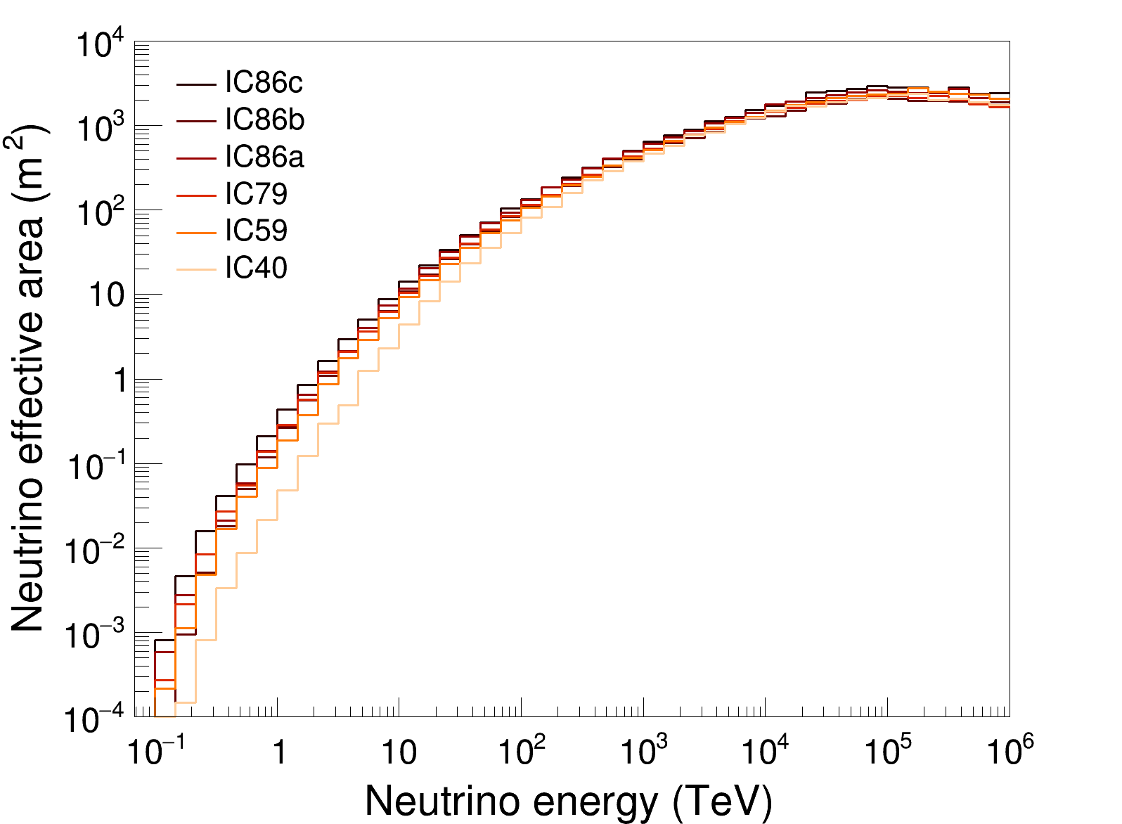
Figure S1: Effective areas for each data sample. Each curve represents the effective area of IceCube to muon neutrino events at the declination of TXS 0506+056 for the different detector configurations.

www.sciencemag.org
Materials and Methods
Figs. S1 – S6

IceCube Collaboration^∗:

M. G. Aartsen¹⁶, M. Ackermann⁵¹, J. Adams¹⁶, J. A. Aguilar¹², M. Ahlers²⁰, M. Ahrens⁴³, I. Al Samarai²⁵, D. Altmann²⁴, K. Andeen³³, T. Anderson⁴⁸, I. Ansseau¹², G. Anton²⁴, C. Argüelles¹⁴, B. Arsioli⁵⁷, J. Auffenberg¹, S. Axani¹⁴, H. Bagherpour¹⁶, X. Bai⁴⁰, J. P. Barron²³, S. W. Barwick²⁷, V. Baum³², R. Bay⁸, J. J. Beatty^18, 19, J. Becker Tjus¹¹, K.-H. Becker⁵⁰, S. BenZvi⁴², D. Berley¹⁷, E. Bernardini⁵¹, D. Z. Besson²⁸, G. Binder^9, 8, D. Bindig⁵⁰, E. Blaufuss¹⁷, S. Blot⁵¹, C. Bohm⁴³, M. Börner²¹, F. Bos¹¹, S. Böser³², O. Botner⁴⁹, E. Bourbeau²⁰, J. Bourbeau³¹, F. Bradascio⁵¹, J. Braun³¹, M. Brenzke¹, H.-P. Bretz⁵¹, S. Bron²⁵, J. Brostean-Kaiser⁵¹, A. Burgman⁴⁹, R. S. Busse³¹, T. Carver²⁵, E. Cheung¹⁷, D. Chirkin³¹, A. Christov²⁵, K. Clark²⁹, L. Classen³⁵, S. Coenders³⁴, G. H. Collin¹⁴, J. M. Conrad¹⁴, P. Coppin¹³, P. Correa¹³, D. F. Cowen^48, 47, R. Cross⁴², P. Dave⁶, M. Day³¹, J. P. A. M. de André²², C. De Clercq¹³, J. J. DeLaunay⁴⁸, H. Dembinski³⁶, S. De Ridder²⁶, P. Desiati³¹, K. D. de Vries¹³, G. de Wasseige¹³, M. de With¹⁰, T. DeYoung²², J. C. Díaz-Vélez³¹, V. di Lorenzo³², H. Dujmovic⁴⁵, J. P. Dumm⁴³, M. Dunkman⁴⁸, E. Dvorak⁴⁰, B. Eberhardt³², T. Ehrhardt³², B. Eichmann¹¹, P. Eller⁴⁸, P. A. Evenson³⁶, S. Fahey³¹, A. R. Fazely⁷, J. Felde¹⁷, K. Filimonov⁸, C. Finley⁴³, S. Flis⁴³, A. Franckowiak⁵¹, E. Friedman¹⁷, A. Fritz³², T. K. Gaisser³⁶, J. Gallagher³⁰, L. Gerhardt⁹, K. Ghorbani³¹, P. Giommi^{54, 55, 56}, T. Glauch³⁴, T. Glüsenkamp²⁴, A. Goldschmidt⁹, J. G. Gonzalez³⁶, D. Grant²³, Z. Griffith³¹, C. Haack¹, A. Hallgren⁴⁹, F. Halzen³¹, K. Hanson³¹, D. Hebecker¹⁰, D. Heereman¹², K. Helbing⁵⁰, R. Hellauer¹⁷, S. Hickford⁵⁰, J. Hignight²², G. C. Hill², K. D. Hoffman¹⁷, R. Hoffmann⁵⁰, T. Hoinka²¹, B. Hokanson-Fasig³¹, K. Hoshina^31, 59, F. Huang⁴⁸, M. Huber³⁴, K. Hultqvist⁴³, M. Hünnefeld²¹, R. Hussain³¹, S. In⁴⁵, N. Iovine¹², A. Ishihara¹⁵, E. Jacobi⁵¹, G. S. Japaridze⁵, M. Jeong⁴⁵, K. Jero³¹, B. J. P. Jones⁴, P. Kalaczynski¹, W. Kang⁴⁵, A. Kappes³⁵, D. Kappesser³², T. Karg⁵¹, A. Karle³¹, U. Katz²⁴, M. Kauer³¹, A. Keivani⁴⁸, J. L. Kelley³¹, A. Kheirandish³¹, J. Kim⁴⁵, M. Kim¹⁵, T. Kintscher⁵¹, J. Kiryluk⁴⁴, T. Kittler²⁴, S. R. Klein^9, 8, R. Koirala³⁶, H. Kolanoski¹⁰, L. Köpke³², C. Kopper²³, S. Kopper⁴⁶, J. P. Koschinsky¹, D. J. Koskinen²⁰, M. Kowalski^10, 51, B. Krammer³⁴, K. Krings³⁴, M. Kroll¹¹, G. Krückl³², S. Kunwar⁵¹, N. Kurahashi³⁹, T. Kuwabara¹⁵, A. Kyriacou², M. Labare²⁶, J. L. Lanfranchi⁴⁸, M. J. Larson²⁰, F. Lauber⁵⁰, K. Leonard³¹, M. Lesiak-Bzdak⁴⁴, M. Leuermann¹, Q. R. Liu³¹, C. J. Lozano Mariscal³⁵, L. Lu¹⁵, J. Lünemann¹³, W. Luszczak³¹, J. Madsen⁴¹, G. Maggi¹³, K. B. M. Mahn²², S. Mancina³¹, R. Maruyama³⁷, K. Mase¹⁵, R. Maunu¹⁷, K. Meagher¹², M. Medici²⁰, M. Meier²¹, T. Menne²¹, G. Merino³¹, T. Meures¹², S. Miarecki^9, 8, J. Micallef²², G. Momenté³², T. Montaruli²⁵, R. W. Moore²³, R. Morse³¹, M. Moulai¹⁴, R. Nahnhauer⁵¹, P. Nakarmi⁴⁶, U. Naumann⁵⁰, G. Neer²², H. Niederhausen⁴⁴, S. C. Nowicki²³, D. R. Nygren⁹, A. Obertacke Pollmann⁵⁰, A. Olivas¹⁷, A. O’Murchadha¹², E. O’Sullivan⁴³, P. Padovani⁵³, T. Palczewski^9, 8, H. Pandya³⁶, D. V. Pankova⁴⁸, P. Peiffer³², J. A. Pepper⁴⁶, C. Pérez de los Heros⁴⁹, D. Pieloth²¹, E. Pinat¹², M. Plum³³, P. B. Price⁸, G. T. Przybylski⁹, C. Raab¹², L. Rädel¹, M. Rameez²⁰, K. Rawlins³, I. C. Rea³⁴, R. Reimann¹, B. Relethford³⁹, M. Relich¹⁵, E. Resconi³⁴, W. Rhode²¹, M. Richman³⁹, S. Robertson², M. Rongen¹, C. Rott⁴⁵, T. Ruhe²¹, D. Ryckbosch²⁶, D. Rysewyk²², I. Safa³¹, N. Sahakyan⁵⁸, T. Sälzer¹, S. E. Sanchez Herrera²³, A. Sandrock²¹, J. Sandroos³², M. Santander⁴⁶, S. Sarkar^20, 38, S. Sarkar²³, K. Satalecka⁵¹, P. Schlunder²¹, T. Schmidt¹⁷, A. Schneider³¹, S. Schoenen¹, S. Schöneberg¹¹, L. Schumacher¹, S. Sclafani³⁹, D. Seckel³⁶, S. Seunarine⁴¹, J. Soedingrekso²¹, D. Soldin³⁶, M. Song¹⁷, G. M. Spiczak⁴¹, C. Spiering⁵¹, J. Stachurska⁵¹, M. Stamatikos¹⁸, T. Stanev³⁶, A. Stasik⁵¹, J. Stettner¹, A. Steuer³², T. Stezelberger⁹, R. G. Stokstad⁹, A. Stößl¹⁵, N. L. Strotjohann⁵¹, T. Stuttard²⁰, G. W. Sullivan¹⁷, M. Sutherland¹⁸, I. Taboada⁶, J. Tatar^9, 8, F. Tenholt¹¹, S. Ter-Antonyan⁷, A. Terliuk⁵¹, S. Tilav³⁶, P. A. Toale⁴⁶, M. N. Tobin³¹, C. Toennis⁴⁵, S. Toscano¹³, D. Tosi³¹, M. Tselengidou²⁴, C. F. Tung⁶, A. Turcati³⁴, C. F. Turley⁴⁸, B. Ty³¹, E. Unger⁴⁹, M. Usner⁵¹, J. Vandenbroucke³¹, W. Van Driessche²⁶, D. van Eijk³¹, N. van Eijndhoven¹³, S. Vanheule²⁶, J. van Santen⁵¹, E. Vogel¹, M. Vraeghe²⁶, C. Walck⁴³, A. Wallace², M. Wallraff¹, F. D. Wandler²³, N. Wandkowsky³¹, A. Waza¹, C. Weaver²³, M. J. Weiss⁴⁸, C. Wendt³¹, J. Werthebach³¹, S. Westerhoff³¹, B. J. Whelan², N. Whitehorn⁵², K. Wiebe³², C. H. Wiebusch¹, L. Wille³¹, D. R. Williams⁴⁶, L. Wills³⁹, M. Wolf³¹, J. Wood³¹, T. R. Wood²³, K. Woschnagg⁸, D. L. Xu³¹, X. W. Xu⁷, Y. Xu⁴⁴, J. P. Yanez²³, G. Yodh²⁷, S. Yoshida¹⁵, T. Yuan<sup>31

1</sup> III. Physikalisches Institut, RWTH Aachen University, D-52056 Aachen, Germany
² Department of Physics, University of Adelaide, Adelaide, 5005, Australia
³ Dept. of Physics and Astronomy, University of Alaska Anchorage, 3211 Providence Dr., Anchorage, AK 99508, USA
⁴ Dept. of Physics, University of Texas at Arlington, 502 Yates St., Science Hall Rm 108, Box 19059, Arlington, TX 76019, USA
⁵ CTSPS, Clark-Atlanta University, Atlanta, GA 30314, USA
⁶ School of Physics and Center for Relativistic Astrophysics, Georgia Institute of Technology, Atlanta, GA 30332, USA
⁷ Dept. of Physics, Southern University, Baton Rouge, LA 70813, USA
⁸ Dept. of Physics, University of California, Berkeley, CA 94720, USA
⁹ Lawrence Berkeley National Laboratory, Berkeley, CA 94720, USA
¹⁰ Institut für Physik, Humboldt-Universität zu Berlin, D-12489 Berlin, Germany
¹¹ Fakultät für Physik & Astronomie, Ruhr-Universität Bochum, D-44780 Bochum, Germany
¹² Université Libre de Bruxelles, Science Faculty CP230, B-1050 Brussels, Belgium
¹³ Vrije Universiteit Brussel (VUB), Dienst ELEM, B-1050 Brussels, Belgium
¹⁴ Dept. of Physics, Massachusetts Institute of Technology, Cambridge, MA 02139, USA
¹⁵ Dept. of Physics and Institute for Global Prominent Research, Chiba University, Chiba 263-8522, Japan
¹⁶ Dept. of Physics and Astronomy, University of Canterbury, Private Bag 4800, Christchurch, New Zealand
¹⁷ Dept. of Physics, University of Maryland, College Park, MD 20742, USA
¹⁸ Dept. of Physics and Center for Cosmology and Astro-Particle Physics, Ohio State University, Columbus, OH 43210, USA
¹⁹ Dept. of Astronomy, Ohio State University, Columbus, OH 43210, USA
²⁰ Niels Bohr Institute, University of Copenhagen, DK-2100 Copenhagen, Denmark
²¹ Dept. of Physics, TU Dortmund University, D-44221 Dortmund, Germany
²² Dept. of Physics and Astronomy, Michigan State University, East Lansing, MI 48824, USA
²³ Dept. of Physics, University of Alberta, Edmonton, Alberta, Canada T6G 2E1
²⁴ Erlangen Centre for Astroparticle Physics, Friedrich-Alexander-Universität Erlangen-Nürnberg, D-91058 Erlangen, Germany
²⁵ Département de physique nucléaire et corpusculaire, Université de Genève, CH-1211 Genève, Switzerland
²⁶ Dept. of Physics and Astronomy, University of Gent, B-9000 Gent, Belgium
²⁷ Dept. of Physics and Astronomy, University of California, Irvine, CA 92697, USA
²⁸ Dept. of Physics and Astronomy, University of Kansas, Lawrence, KS 66045, USA
²⁹ SNOLAB, 1039 Regional Road 24, Creighton Mine 9, Lively, ON, Canada P3Y 1N2
³⁰ Dept. of Astronomy, University of Wisconsin, Madison, WI 53706, USA
³¹ Dept. of Physics and Wisconsin IceCube Particle Astrophysics Center, University of Wisconsin, Madison, WI 53706, USA
³² Institute of Physics, University of Mainz, Staudinger Weg 7, D-55099 Mainz, Germany
³³ Department of Physics, Marquette University, Milwaukee, WI, 53201, USA
³⁴ Physik-department, Technische Universität München, D-85748 Garching, Germany
³⁵ Institut für Kernphysik, Westfälische Wilhelms-Universität Münster, D-48149 Münster, Germany
³⁶ Bartol Research Institute and Dept. of Physics and Astronomy, University of Delaware, Newark, DE 19716, USA
³⁷ Dept. of Physics, Yale University, New Haven, CT 06520, USA
³⁸ Dept. of Physics, University of Oxford, 1 Keble Road, Oxford OX1 3NP, UK
³⁹ Dept. of Physics, Drexel University, 3141 Chestnut Street, Philadelphia, PA 19104, USA
⁴⁰ Physics Department, South Dakota School of Mines and Technology, Rapid City, SD 57701, USA
⁴¹ Dept. of Physics, University of Wisconsin, River Falls, WI 54022, USA
⁴² Dept. of Physics and Astronomy, University of Rochester, Rochester, NY 14627, USA
⁴³ Oskar Klein Centre and Dept. of Physics, Stockholm University, SE-10691 Stockholm, Sweden
⁴⁴ Dept. of Physics and Astronomy, Stony Brook University, Stony Brook, NY 11794-3800, USA
⁴⁵ Dept. of Physics, Sungkyunkwan University, Suwon 440-746, Korea
⁴⁶ Dept. of Physics and Astronomy, University of Alabama, Tuscaloosa, AL 35487, USA
⁴⁷ Dept. of Astronomy and Astrophysics, Pennsylvania State University, University Park, PA 16802, USA
⁴⁸ Dept. of Physics, Pennsylvania State University, University Park, PA 16802, USA
⁴⁹ Dept. of Physics and Astronomy, Uppsala University, Box 516, S-75120 Uppsala, Sweden
⁵⁰ Dept. of Physics, University of Wuppertal, D-42119 Wuppertal, Germany
⁵¹ DESY, D-15738 Zeuthen, Germany
⁵² Dept. of Physics and Astronomy, University of California, Los Angeles, CA 90095, USA
⁵³ European Southern Observatory, Karl-Schwarzschild-Str. 2, D-85748 Garching bei München, Germany
⁵⁴ ASI, via del Politecnico s.n.c., I-00133 Roma, Italy
⁵⁵ Institute for Advanced Studies, Technische Universität München, Lichtenbergstrasse 2a, D-85748 Garching bei München, Germany
⁵⁶ ICRANet, Piazzale della Repubblica, 10 - 65122, Pescara, Italy
⁵⁷ Instituto de Física Gleb Wataghin, UNICAMP, R. Sérgio Buarque de Holanda 777, 13083-859 Campinas, Brazil
⁵⁸ ICRANet-Armenia, Marshall Baghramian Avenue 24a, 0019 Yerevan, Republic of Armenia
⁵⁹ Earthquake Research Institute, University of Tokyo, Bunkyo, Tokyo 113-0032, Japan

^∗E-mail: analysis@icecube.wisc.edu

Materials and Methods

Time-integrated analysis method

The time-integrated analysis uses the unbinned maximum likelihood technique described in  (?) to quantify spatial clustering of neutrino events on the sky. Energy information is also used in the analysis, primarily as a means to help separate signal and background rather than to characterize the energy distribution of the neutrino signal itself. In this method the unbinned likelihood is defined as a product over all neutrino events in the data sample:

$$\mathcal{L}(\Phi_{100},\gamma)=\prod_{i}\Big{(}\frac{n_{S}(\Phi_{100},\gamma)}{N}\mathcal{S}(\mathbf{x}_{S},\mathbf{x}_{i},\sigma_{i},E_{i};\gamma)+\Big{(}1-\frac{n_{S}(\Phi_{100},\gamma)}{N}\Big{)}\mathcal{B}(\mathrm{sin}\,\delta_{i},E_{i})\Big{)}$$ (S1)

where $\mathcal{S}$ represents the probability distribution function (PDF) of signal events from a point source, $\mathcal{B}$ represents the PDF of background events, $N$ is the total number of neutrino events, and $n_{S}(\Phi_{100},\gamma)$ is the corresponding number of signal neutrinos in the sample for a signal flux model of the form $\Phi(E)=\Phi_{100}(E/100\,\mathrm{TeV})^{-\gamma}$ where $E$ is the true neutrino energy, $\gamma$ is the spectral index, and $\Phi_{100}$ is the flux normalization at 100 TeV.

$\mathcal{S}$ depends on the position of the source $\mathbf{x}_{S}$, given as a vector in right ascension and declination, the reconstructed direction of the neutrino event $\mathbf{x}_{i}$, and the spectral index $\gamma$ from the power-law flux model. It can be factorized into a spatial component and an energy component. The spatial component is described by a two-dimensional Gaussian, exp$(-\lvert\mathbf{x}_{S}-\mathbf{x}_{i}\rvert^{2}/2\,\sigma_{i}^{2})\,/\,2\pi\sigma_{i}^{2}$, where $\sigma_{i}$ is the directional reconstruction uncertainty for the $i^{\mathrm{th}}$ neutrino event. The energy component $\mathcal{E}_{S}(E_{i},\mathrm{sin}\,\delta_{i};\gamma)$ accounts for the probability of observing a neutrino event with reconstructed energy $E_{i}$ (muon energy proxy, defined below), at a reconstructed declination of $\delta_{i}$ for the signal flux model with spectral index $\gamma$. $\mathcal{E}_{S}$ is a function of declination because the effective area of IceCube is declination dependent.The full form is:

$$\mathcal{S}(\mathbf{x}_{S},\mathbf{x}_{i},\sigma_{i},E_{i};\gamma)=\frac{1}{2\pi\sigma_{i}^{2}}\,\mathrm{e}^{-\frac{\lvert\mathbf{x}_{S}-\mathbf{x}_{i}\rvert^{2}}{2\sigma_{i}^{2}}}\times\mathcal{E}_{S}(E_{i},\mathrm{sin}\,\delta_{i};\gamma).$$ (S2)

We construct $\mathcal{B}$ from individual spatial and energy components for background events as well. The spatial term is estimated using experimental data and depends only on the event’s declination $\delta_{i}$, because the probability distribution of background events is uniform in right ascension. The spatial PDF for background, $\mathcal{P_{B}}(\mathrm{sin}\,\delta_{i})$, is equal to the event density per solid angle, divided by the total number of events in the sample. The background energy PDF $\mathcal{E}_{B}(E_{i},\mathrm{sin}\,\delta_{i})$ is also estimated directly from experimental data by measuring the fraction of events with energy proxy $E_{i}$ at a reconstructed declination of $\mathrm{sin}\,\delta_{i}$. The full form of $\mathcal{B}$ is:

$$\mathcal{B}(\mathrm{sin}\,\delta_{i},E_{i})=\mathcal{P}_{\mathcal{B}}(\mathrm{sin}\,\delta_{i})\times\mathcal{E}_{B}(E_{i},\mathrm{sin}\,\delta_{i}).$$ (S3)

The ratio $\mathcal{S}/\mathcal{B}$ evaluated for a single event is referred to as the Event Weight. The main contribution to the likelihood and the final significance comes from events with large values of $\mathcal{S}/\mathcal{B}$ (see e.g. Fig. 2). For a given $\Phi(E)$, the number of signal events $n_{S}$ expected in the data depends upon the exposure time $T$ and the declination-dependent effective area, $A_{eff}(E,\mathrm{sin}\,\delta_{i})$, that characterizes the detector and data sample. It is given by:

$$n_{S}=T\times\int_{100\,\mathrm{GeV}}^{1\,\mathrm{EeV}}A_{eff}(E,\mathrm{sin}\,\delta_{i})\,\Phi(E)dE$$ (S4)

where the integration is over the range of true neutrino energies relevant for the data samples. We calculate $n_{S}(\Phi_{100},\gamma)$ from Eq. S4 for the case where $\Phi(E)=\Phi_{100}(E/100\,\mathrm{TeV})^{-\gamma}$.

Properties such as effective area and exposure time vary for each of the data samples shown in Table 1, so we compute $\mathcal{L}$ separately for each, and combine them as a product:

$$\mathcal{L}(\Phi_{100},\gamma)=\prod_{j}\mathcal{L}_{j}(\Phi_{100},\gamma)$$ (S5)

where $j$ denotes the data sample. The case $\mathcal{L}(\Phi_{100}=0)$ represents the null hypothesis of no point source signal present (in which case $\gamma$ is not defined). We form the test statistic $TS=2\,\mathrm{log}(\mathcal{L}(\Phi_{100},\gamma)/\mathcal{L}(\Phi_{100}=0))$ as a likelihood ratio relative to the null hypothesis and maximize it as a function of its two parameters over the ranges $\Phi_{100}\geq 0$, $\gamma\in[1,4]$ to find the best-fitting values of $\Phi_{100}$ and $\gamma$.

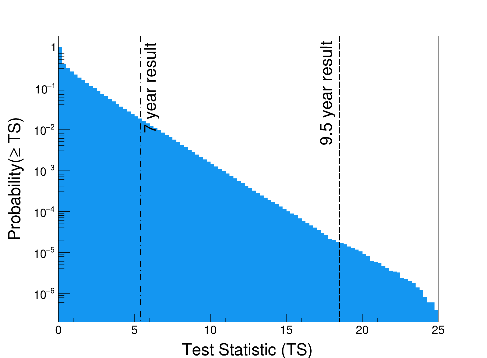
Figure S2: Time-integrated analysis test statistic distribution. The blue curve corresponds to the probability of observing at least the test statistic value $TS$ from the time-integrated analysis performed on randomized data. The dashed line marks the $TS$ value observed at the location of TXS 0506+056 with 9.5 years of data, including the IceCube-170922A event. The dash-dotted line marks the $TS$ value observed at the location of TXS 0506+056 with 7 years of data (IC86c removed), which does not contain the IceCube-170922A event.

We estimate the probability distribution of the test statistic under the null hypothesis by performing the time-integrated analysis at the location of TXS 0506+056 on samples of randomized data. Each sample is produced by assigning random values of right ascension, from 0^∘ to 360^∘, to events in the original data set with a random number generator. The significance of the result for the real data is given by the p-value, defined as the fraction of randomized trials with $TS\geq TS_{\mathrm{data}}$. The test-statistic distribution for the time-integrated analysis performed on 5 million randomized data sets is shown in Fig. S2. The advantage of using randomized experimental data samples to simulate the null hypothesis is that the resulting significance estimate is generally conservative and robust against systematic errors due for example to imperfect detector simulation of the background.

Time-dependent analysis method

The time-dependent analysis uses the unbinned maximum-likelihood technique described in  (?) to search for a point source signal in which the neutrinos also cluster in time. In the model-independent version of this analysis, minimal assumptions about the time structure of the neutrino signal are made. It is only assumed that the emission is clustered around some time $T_{0}$ with some duration $T_{\mathrm{W}}$, where these are parameter values to be determined by the best fit to the data. As with the use of energy information in the analysis, the search for time-clustering is primarily a way to improve the chance of identifying a possibly time-dependent neutrino signal, rather than to provide a detailed characterization of time variability.

We consider two functional forms for the temporal distribution of events, a box function and a one-dimensional Gaussian function. These both provide reasonable fits to generic transient signals in the low statistics regime where the small number of recorded signal events provide minimal information about the exact shape. The box function is given by

$$\mathcal{T}_{S}(t_{i};T_{0},T_{\mathrm{W}})=\frac{1}{T_{\mathrm{W}}}\quad(T_{0}-T_{\mathrm{W}}/2<t_{i}<T_{0}+T_{\mathrm{W}}/2)\quad\mathrm{BOX}$$ (S6)

where $T_{0}$ is the central time and $T_{\mathrm{W}}$ is the full width of the box shape. The Gaussian shape is described by the same parameters but with the following functional form

$$\mathcal{T}_{S}(t_{i};T_{0},T_{\mathrm{W}})=\frac{1}{\sqrt{2\pi(T_{\mathrm{W}}/2)^{2}}}\,e^{-\frac{(t_{i}-T_{0})^{2}}{2(T_{\mathrm{W}}/2)^{2}}}\quad\mathrm{GAUSSIAN}$$ (S7)

The PDF for the time distribution of background events $\mathcal{T}_{B}$ is given to good approximation by $1/T$, where $T$ is the total observation time of the data sample, because IceCube maintains essentially uniform efficiency with time during each individual observation period  (?).

The unbinned likelihood for this method is similar to the time-integrated likelihood with the functions $\mathcal{S}$ and $\mathcal{B}$ defined as before, and now including signal and background temporal terms. It is defined as a product over all neutrino events in the data sample

$$\mathcal{L}(\Phi_{100},\gamma,T_{0},T_{\mathrm{W}})=\prod_{i}\Big{(}\frac{n_{S}(\Phi_{100},\gamma)}{N}\mathcal{S}\times\mathcal{T}_{S}(t_{i};T_{0},T_{\mathrm{W}})+\Big{(}1-\frac{n_{S}(\Phi_{100},\gamma)}{N}\Big{)}\mathcal{B}\times\mathcal{T}_{B}\Big{)}.$$ (S8)

We compute the time-dependent likelihood separately for each of the data periods shown in Table 1 under the assumption that we are looking for neutrino emission on timescales less than the $\sim$ year durations of the data sets. This is because significant emission on longer timescales will appear in the time-integrated analysis. As before, the test statistic is constructed using a likelihood ratio of the signal and null hypotheses:

$$TS=2\,\mathrm{log}\Big{[}\,\frac{T_{\mathrm{W}}}{\mathrm{T}}\times\frac{\mathcal{L}(\Phi_{100},\gamma,T_{0},T_{\mathrm{W}})}{\mathcal{L}(\Phi_{100}=0)}\,\Big{]}$$ (S9)

where the additional factor $T_{\mathrm{W}}/\mathrm{T}$ corrects for the look-elsewhere effect due to choosing a time window of width $T_{\mathrm{W}}$ from within a sample with observation time $T$. As explained in  (?) where it is derived, the form of this correction arises from the fact that there are more possible short time windows than long ones, with correspondingly more possibilities for a cluster to occur in a short window by chance. We maximize the test statistic as a function of its four parameters in order to find the best-fit values of $\Phi_{100}$, $\gamma$, $T_{\mathrm{W}}$, and $T_{0}$. This is done over the ranges $\Phi_{100}\geq 0$, $\gamma\in[1,4]$, $T_{\mathrm{W}}<T/2$, $T_{0}\in[T_{\mathrm{min}},T_{\mathrm{max}}]$ where $T_{\mathrm{min}}$ and $T_{\mathrm{max}}$ are the start and end times of the data sample.

Again, we estimate the probability distribution of the test statistic under the null hypothesis by performing the time-dependent analysis at the location of TXS 0506+056 on samples of randomized data. In the time-dependent case, random samples are produced by randomly re-assigning the times among the events within the same data period used to compute the likelihood. The equatorial coordinates are then recomputed using the new times. All other event properties remain unchanged. Fig. S3 shows the resulting test-statistic distributions for the analysis applied to randomized IC86b data samples using both the box and the Gaussian window shapes.

Since we perform the likelihood analysis separately on six data samples, there is an additional look-elsewhere correction when we choose the sample with the best p-value. For small p-values (i.e. if the result is significant) this correction can be made by multiplying the p-value by $T_{\mathrm{total}}/T$, where $T$ is the observation time of the chosen sample, and $T_{\mathrm{total}}$ is the combined observation time of all of the samples. This is an extension of the same look-elsewhere factor described above, from  (?).

Muon energy and neutrino energy

While traversing the ice, muons above $\sim 1$ TeV experience stochastic energy losses due to pair production, bremsstrahlung, and photo-nuclear interactions. The magnitude of these energy losses is inferred from the pattern and intensity of Cherenkov photons recorded by the optical sensors, allowing an estimate of the muon’s energy. Inferring the energy of the original neutrino from the muon energy introduces significant uncertainties, because the muon can travel kilometers in the ice and only part of the track is observed as it passes through the instrumented detector volume. In most cases, the muon is created in a neutrino interaction that occurred at an unknown distance before the muon arrived at the detector region, so the observed muon energy that remains is in general a lower bound on the neutrino energy.

The likelihood analysis does not attempt to estimate the original neutrino energy for each event. Instead, for the signal energy PDF, it relies on the distribution of expected muon energies which is determined by detector simulation using the neutrino flux model specified in the signal hypothesis. The background energy PDF is determined by the muon energy distribution of the experimental data itself. This allows the likelihood ratio test to be performed directly using the reconstructed muon-energy observables.

For a single event, it is possible to use the reconstructed muon energy to estimate the original neutrino energy, with large uncertainties. Fig. S4 shows an example of the distribution of reconstructed muon energies for a range of different neutrino energies based on detector simulations of the IC86b sample for neutrinos arriving from the declination of TXS 0506+056. Given the reconstructed muon energy of a single event, the probability distribution for the original neutrino energy depends on the assumed prior distribution of neutrino energies. In Fig. S5 this is shown for the same simulation and assuming that the neutrino flux follows a power-law spectrum $dN/dE\propto E^{-2.1}$. A specific example for the case of a reconstructed muon energy of 10 TeV in the IC86b sample, at the declination of TXS 0506+056, is shown in Fig. S6 for different assumed power-law spectra.

The muon energy reconstruction algorithms are different across the six data samples, as are the expected distributions of muon energies due to different event selections and detector configurations. The muon energy observable is generically referred to as the Muon Energy Proxy, but it is strictly only comparable with other proxy values from the same data sample. Details of the event selections and reconstruction algorithms for each sample are described in  (?) and references therein.

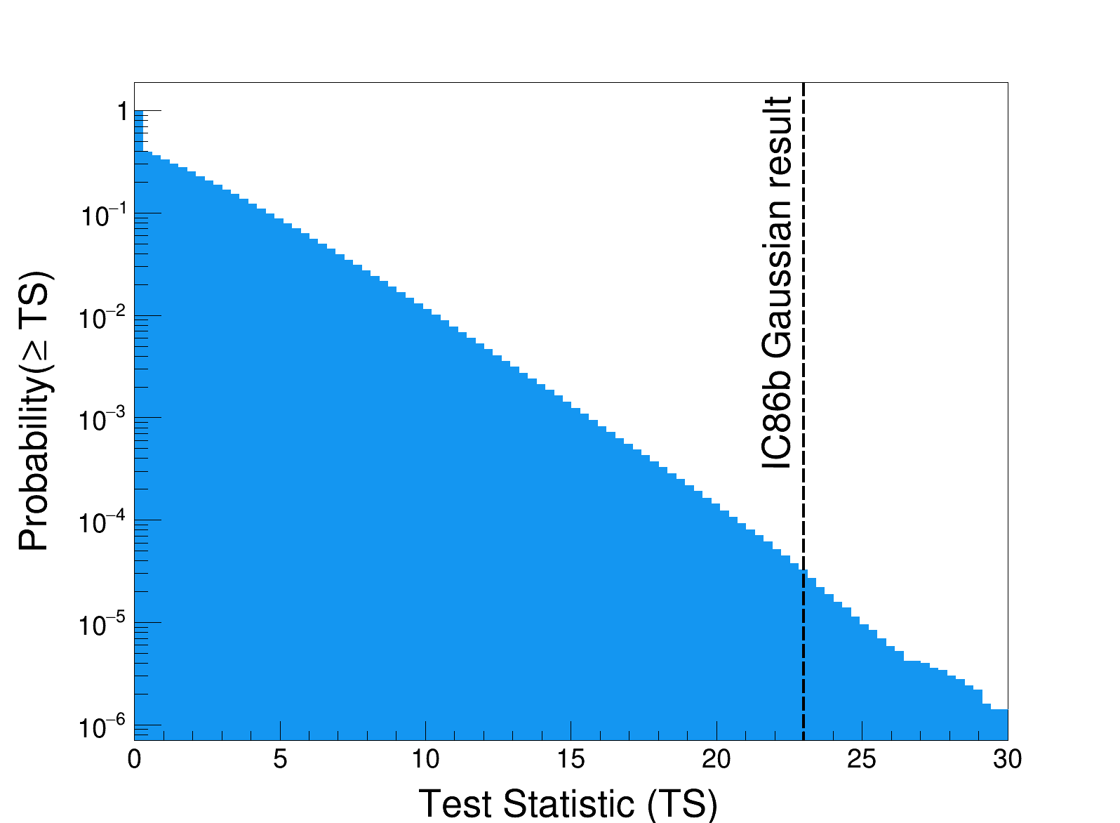
(a)

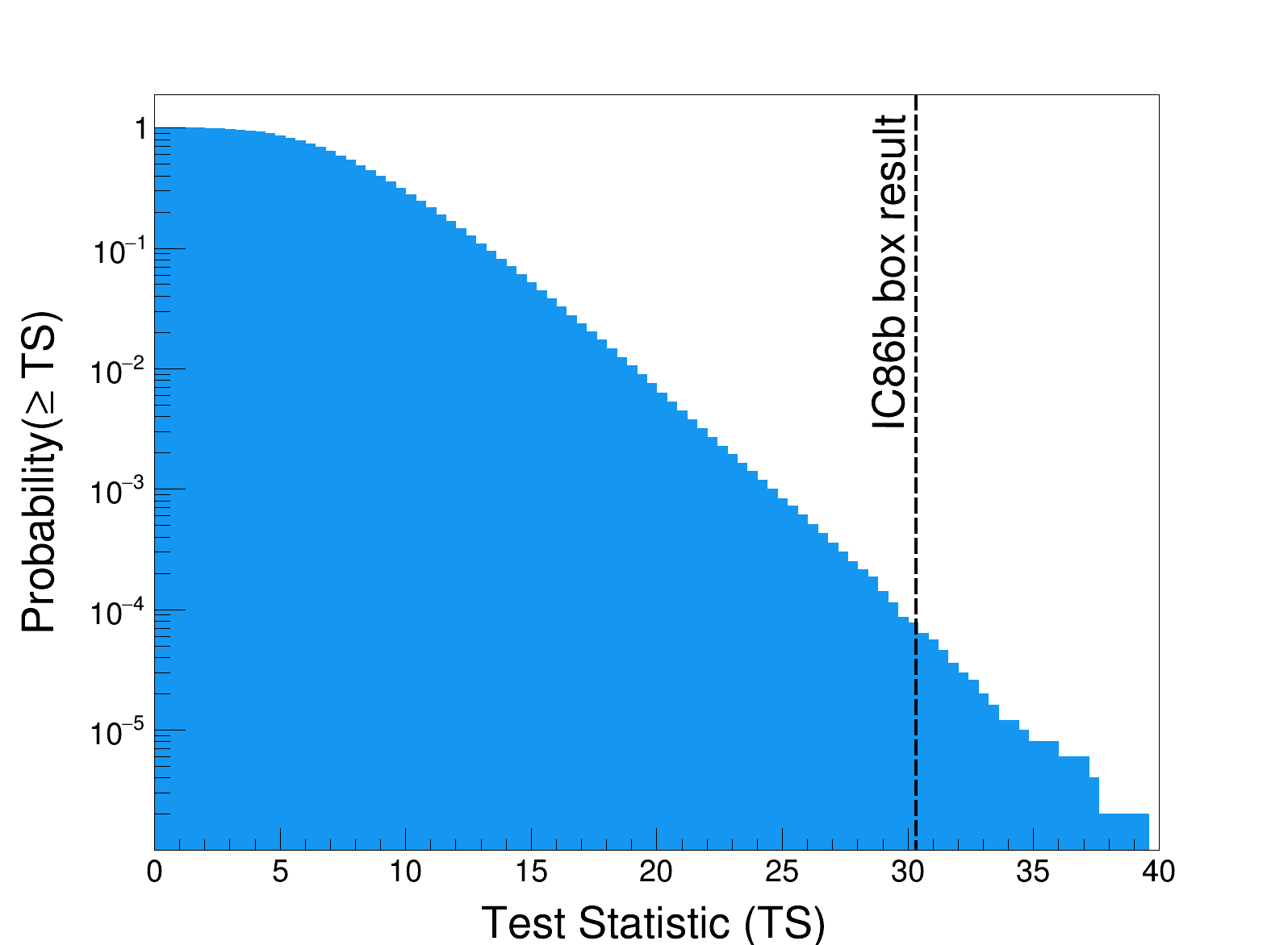
(b)

Figure S3: Time-dependent analysis test statistic distributions. The blue curve corresponds to the probability of observing at least the test statistic value $TS$ from the time-dependent analysis performed on randomized data with (a) the Gaussian window and (b) the box window. The dashed lines mark the $TS$ values observed at the location of TXS 0506+056 with the Gaussian and box windows during the IC86b period.

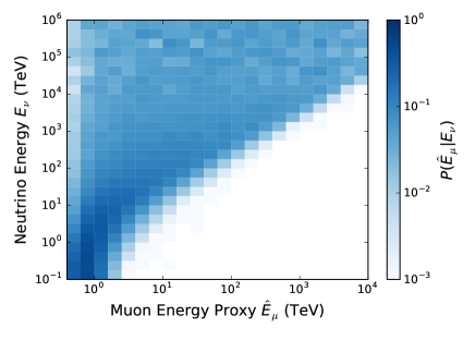
Figure S4: Distribution of Muon Energy Proxy for true neutrino energies. Distribution of reconstructed muon energies (Muon Energy Proxy) for different neutrino energies specified on the y-axis. Each horizontal slice in neutrino energy $E_{\nu}$ has been individually normalized. The neutrinos were simulated from the declination of TXS 0506+056 with the same event selection and reconstruction algorithms as applied to the real data for the IC86b sample.

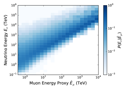
Figure S5: Distribution of true neutrino energy as a function of Muon Energy Proxy. Distribution of true neutrino energies for different observed values of the Muon Energy Proxy specified on the x-axis. The same simulation was used for IC86b as in Fig. S4, with the neutrino energy distribution weighted according to a power-law spectrum $dN/dE\propto E^{-2.1}$. Each vertical slice in Muon Energy Proxy was then individually normalized. Assuming this prior on the neutrino energy distribution, an observed value of the Muon Energy Proxy determines the probability distribution of the true neutrino energy.

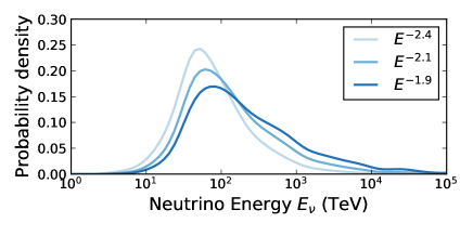
Figure S6: Estimate of neutrino energy for Muon Energy Proxy of 10 TeV. Probability distribution of neutrino energies corresponding to a Muon Energy Proxy value of 10 TeV, under different assumptions of the neutrino spectral energy distribution. The same simulation was used as in Fig. S4.

References

- 1. A. Aab, et al., Science 357, 1266 (2017).
- 2. F. Reines, Ann. Rev. Nucl. Part. Sci. 10, 1 (1960).
- 3. C. M. Urry, P. Padovani, Publications of the Astronomical Society of the Pacific 107, 803 (1995).
- 4. K. Mannheim, Astroparticle Physics 3, 295 (1995).
- 5. F. Halzen, E. Zas, Astrophysical Journal 488, 669 (1997).
- 6. A. Mücke, R. J. Protheroe, R. Engel, J. P. Rachen, T. Stanev, Astroparticle Physics 18, 593 (2003).
- 7. K. Murase, in Neutrino Astronomy, T. Gaisser, A. Karle, Eds. (World Scientific, 2017) pp. 15–31.
- 8. M. Petropoulou, C. Dermer, Astrophysical Journal Letters 825 (2017).
- 9. C. Guépin, K. Kotera, Astronomy & Astrophysics 603 (2017).
- 10. M.-H. Ulrich, L. Maraschi, C. M. Urry, Annual Review of Astronomy and Astrophysics 35, 445 (1997).
- 11. M. G. Aartsen, et al., Journal of Instrumentation 12, P03012 (2017).
- 12. M. G. Aartsen, et al., Astrophysical Journal 835, 151 (2017).
- 13. M. G. Aartsen, et al., Physical Review D89, 102004 (2014).
- 14. IceCube Collaboration, Science 342, 1242856 (2013).
- 15. M. G. Aartsen, et al., Physical Review Letters 113, 101101 (2014).
- 16. M. G. Aartsen, et al., Astrophysical Journal 809, 98 (2015).
- 17. M. G. Aartsen, et al., Astrophysical Journal 833, 3 (2016).
- 18. M. G. Aartsen, et al., Astrophysical Journal 807, 46 (2015).
- 19. E. Massaro, et al., Astrophysics and Space Science 357, 75 (2015).
- 20. M. G. Aartsen, et al., Science this issue (2017).
- 21. M. G. Aartsen, et al., Astroparticle Physics 92, 30 (2017).
- 22. IceCube Collaboration, GRB Coordinates Network, Circular Service 21916 (2017).
- 23. Y. T. Tanaka, S. Buson, D. Kocevski, The Astronomer’s Telegram 10791 (2017).
- 24. W. B. Atwood, et al., Astrophysical Journal 697, 1071 (2009).
- 25. J. Aleksić, et al., Astroparticle Physics 35, 435 (2012).
- 26. R. Mirzoyan, The Astronomer’s Telegram 10817 (2017).
- 27. R. Abbasi, et al., Astrophysical Journal 744, 1 (2012).
- 28. J. Braun, et al., Astroparticle Physics 29, 299 (2008).
- 29. J. Braun, et al., Astroparticle Physics 33, 175 (2010).
- 30. Materials and methods are available as supplementary materials on Science Online.
- 31. K. Meagher, IceCube Collaboration, 35th International Cosmic Ray Conference, Proceedings of Science 301, 1007 (2017).
- 32. S. Paiano, R. Falomo, A. Treves, R. Scarpa, Astrophysical Journal 854, L32 (2018).
- 33. M. Ackermann, et al., Astrophysical Journal 810, 14 (2015).
- 34. M. G. Aartsen, et al., Astrophysical Journal 835, 45 (2017).
- 35. M. Ackermann, et al., Astrophysical Journal 743, 171 (2011).
- 36. S. S. Wilks, Annals Math. Statist. 9, 60 (1938).