Unbiased Markov chain Monte Carlo for intractable target distributions

Abstract

Performing numerical integration when the integrand itself cannot be evaluated point-wise is a challenging task that arises in statistical analysis, notably in Bayesian inference for models with intractable likelihood functions. Markov chain Monte Carlo (MCMC) algorithms have been proposed for this setting, such as the pseudo-marginal method for latent variable models and the exchange algorithm for a class of undirected graphical models. As with any MCMC algorithm, the resulting estimators are justified asymptotically in the limit of the number of iterations, but exhibit a bias for any fixed number of iterations due to the Markov chains starting outside of stationarity. This “burn-in” bias is known to complicate the use of parallel processors for MCMC computations. We show how to use coupling techniques to generate unbiased estimators in finite time, building on recent advances for generic MCMC algorithms. We establish the theoretical validity of some of these procedures, by extending existing results to cover the case of polynomially ergodic Markov chains. The efficiency of the proposed estimators is compared with that of standard MCMC estimators, with theoretical arguments and numerical experiments including state space models and Ising models.

1 Introduction

1.1 Context

For various statistical models the likelihood function cannot be computed point-wise, which prevents the use of standard Markov chain Monte Carlo (MCMC) algorithms such as Metropolis–Hastings (MH) for Bayesian inference. For example, the likelihood of latent variable models typically involves an intractable integral over the latent space. Classically, one can address this problem by designing MCMC algorithms on the joint space of parameters and latent variables. However, these samplers can mix poorly when latent variables and parameters are strongly correlated under the joint posterior distribution. Furthermore these schemes cannot be implemented if we can only simulate the latent variables and not evaluate their probability density function (Andrieu et al., 2010, Section 2.3). Similarly, in the context of undirected graphical models, the likelihood function might involve an intractable integral over the observation space; see Møller et al. (2006) with examples from spatial statistics.

Pseudo-marginal methods have been proposed for these situations (Lin et al., 2000; Beaumont, 2003; Andrieu and Roberts, 2009), whereby unbiased Monte Carlo estimators of the likelihood are used within an MH acceptance mechanism while still producing chains that are ergodic with respect to the exact posterior distribution of interest, denoted by $\pi$. Pseudo-marginal algorithms and their extensions (Deligiannidis et al., 2018; Tran et al., 2016) are particularly adapted to latent variable models, such as random effects models and state space models, where the likelihood can be estimated without bias using importance sampling or particle filters (Beaumont, 2003; Andrieu and Roberts, 2009; Andrieu et al., 2010). Related schemes include the exchange algorithm (Murray et al., 2006; Andrieu et al., 2018), which applies to scenarios where the likelihood involves an intractable, parameter-dependent normalizing constant. Exchange algorithms rely on simulation of synthetic observations to cancel out intractable terms in the MH acceptance ratio. As with any MCMC algorithm, the computation of each iteration requires the completion of the previous ones, which hinders the potential for parallel computation. Running independent chains in parallel is always possible, and averaging over independent chains leads to a linear decrease of the resulting variance. However, the inherent bias that comes from starting the chains outside of stationarity, also called the “burn-in bias”, remains (Rosenthal, 2000).

This burn-in bias has motivated various methodological developments in the MCMC literature; among these, some rely on coupling techniques, such as the circularly-coupled Markov chains of Neal (2017), regeneration techniques described in Mykland et al. (1995); Brockwell and Kadane (2005), and “coupling from the past” as proposed in Propp and Wilson (1996). Coupling methods have also been proposed for diagnosing convergence in Johnson (1996, 1998) and as a means to assess the approximation error for approximate MCMC kernels in Nicholls et al. (2012). Recently, a method has been proposed to completely remove the bias of Markov chain ergodic averages (Glynn and Rhee, 2014). An extension of this approach using coupling ideas was proposed by Jacob et al. (2020) and applied to a variety of MCMC algorithms. This methodology involves the construction of a pair of Markov chains, which are simulated until an event occurs. At this point, a certain function of the chains is returned, with the guarantee that its expectation is exactly the integral of interest. The output is thus an unbiased estimator of that integral. Averaging over i.i.d. copies of such estimators we obtain consistent estimators in the limit of the number of copies, which can be generated independently in parallel. Relevant limit theorems have been established in Glynn and Heidelberger (1990); Glynn and Whitt (1992), enabling the construction of valid confidence intervals. The methodology has already been demonstrated for various MCMC algorithms (Jacob et al., 2020; Heng and Jacob, 2019; Jacob et al., 2019), which were instances of geometrically ergodic Markov chain samplers under typical conditions. However, in the case of intractable likelihoods and pseudo-marginal samplers, in realistic situations the associated Markov chains can often be sub-geometrically ergodic, see e.g. (Andrieu and Vihola, 2015).

We show here that unbiased estimators of $\pi(h)$, with finite variance and finite computational cost, can also be derived from polynomially ergodic Markov chains such as those generated by pseudo-marginal methods. We provide results on the associated efficiency in comparison with standard MCMC estimators. We apply the methodology to particle MCMC algorithms for inference in generic state space models, with an application to a time series of neuron activation counts. We also consider a variant of the pseudo-marginal approach known as the block pseudo-marginal approach (Tran et al., 2016) as well as the exchange algorithm (Murray et al., 2006).

Accompanying code used for simulations and to generate the figures are provided at https://github.com/lolmid/unbiased_intractable_targets.

1.2 Unbiased estimators from coupled Markov chains

Let $\pi$ be a probability measure on a topological space $\mathcal{Z}$ equipped with the Borel $\sigma$-algebra $\mathcal{B}(\mathcal{Z})$. In this section we recall how two coupled chains that are marginally converging to $\pi$ can be used to produce unbiased estimators of expectations $\pi(h):=\int h\left(z\right)\pi(dz)$ for any $\pi$-integrable test function $h:\mathcal{Z}\to\mathbb{R}$. Following Glynn and Rhee (2014); Jacob et al. (2020), we consider the following coupling of two Markov chains $(Z_{n})_{n\geq 0}$ and $(\tilde{Z}_{n})_{n\geq 0}$. First, $Z_{0},\tilde{Z}_{0}$ are drawn independently from an initial distribution $\pi_{0}$. Then, $Z_{1}$ is drawn from a Markov kernel $P$ given $Z_{0}$, which is denoted $Z_{1}|Z_{0}\sim P(Z_{0},\cdot)$. Subsequently, at step $n\geq 1$, a pair $(Z_{n+1},\tilde{Z}_{n})$ is drawn from a Markov kernel $\bar{P}$ given $(Z_{n},\tilde{Z}_{n-1})$, which is denoted $(Z_{n+1},\tilde{Z}_{n})|(Z_{n},\tilde{Z}_{n-1})\sim\bar{P}((Z_{n},\tilde{Z}_{n-1}),\cdot)$. The kernel $\bar{P}$ is such that, marginally, $Z_{n+1}|(Z_{n},\tilde{Z}_{n-1})\sim P(Z_{n},\cdot)$ and $\tilde{Z}_{n}|(Z_{n},\tilde{Z}_{n-1})\sim P(\tilde{Z}_{n-1},\cdot)$. This implies that, marginally for all $n\geq 0$, $Z_{n}$ and $\tilde{Z}_{n}$ have the same distribution. Furthermore, the kernel $\bar{P}$ is constructed so that there exists a random variable $\tau$ termed the meeting time, such that for all $n\geq\tau$, $Z_{n}=\tilde{Z}_{n-1}$ almost surely (a.s.). Then, for any integer $k$, the following informal telescoping sum argument informally suggests an unbiased estimator of $\pi(h)$. We start from $\pi(h)=\lim_{n\to\infty}\mathds{E}[h(Z_{n})]$ and write

$$\pi\left(h\right) =\mathds{E}[h(Z_{k})]+\sum_{n=k+1}^{\infty}\mathds{E}[h(Z_{n})]-\mathds{E}[h(\tilde{Z}_{n-1})] \text{(write as telescoping sum)},$$

$$=\mathds{E}[h(Z_{k})+\sum_{n=k+1}^{\infty}h(Z_{n})-h(\tilde{Z}_{n-1})\text{]} \text{(swap expectation \& limit)},$$

$$=\mathds{E}[h(Z_{k})+\sum_{n=k+1}^{\tau-1}h(Z_{n})-h(\tilde{Z}_{n-1})] \text{($Z_{n}=\tilde{Z}_{n-1}$ for $n\geq\tau$)}.$$

The sum $\sum_{n=k+1}^{\tau-1}$ is treated as zero if $\tau-1<k+1$. The suggested estimator is thus defined as

$$H_{k}(Z,\tilde{Z})=h(Z_{k})+\sum_{n=k+1}^{\tau-1}\{h(Z_{n})-h(\tilde{Z}_{n-1})\},$$ (1)

with $Z$ and $\tilde{Z}$ denoting the chains $(Z_{n})_{n\geq 0}$ and $(\tilde{Z}_{n})_{n\geq 0}$ respectively. As in Jacob et al. (2020), we average $H_{l}(Z,\tilde{Z})$ over a range of values of $l$, $l\in\{k,k+1,...,m\}$ for an integer $m\geq k$, resulting in the estimator

$$H_{k:m}(Z,\tilde{Z})=\frac{1}{m-k+1}\sum_{l=k}^{m}h(Z_{l})+\sum_{n=k+1}^{\tau-1}\min\left(1,\frac{n-k}{m-k+1}\right)(h(Z_{n})-h(\tilde{Z}_{n-1})).$$ (2)

Intuitively, $H_{k:m}$ can be understood as a standard Markov chain average after $m$ steps using a burn-in period of $k-1$ steps (which would be in general biased for $\pi(h)$), plus a second term that can be shown to remove the burn-in bias. That “bias correction” term is a weighted sum of differences of the chains between step $k$ and the meeting time $\tau=\inf\{n\geq 1:\;Z_{n}=\tilde{Z}_{n-1}\}$. In the following, we will write $H_{k:m}:=H_{k:m}(Z,\tilde{Z})$ for brevity. The construction of $H_{k:m}$ is summarized in Algorithm 1, where the initial distribution of the chains is denoted by $\pi_{0}$, and the Markov kernels by $P$ and $\bar{P}$ as above. Standard MCMC estimators require the specification of $\pi_{0}$ and $P$, while the proposed method requires the additional specification of the coupled kernel $\bar{P}$. We will propose coupled kernels for the setting of intractable likelihoods, and study the estimator $H_{k:m}$ under conditions which cover pseudo-marginal methods.

Algorithm 1 Unbiased MCMC estimator $H_{k:m}$ for any choice of $k$ and $m$ with $0\leq k\leq m$.

1. Initialization:

   1. Sample $Z_{0},\tilde{Z}_{0}\sim\pi_{0}$$\left(\cdot\right)$.

   2. Sample $Z_{1}|\{Z_{0}=z_{0}\}\sim P(z_{0},\cdot)$.

   3. Set $n=1$ and $\tau=\infty$.

2. While $n<\max(m,\tau)$:

   1. Sample $(Z_{n+1},\tilde{Z}_{n})|\{Z_{n}=z_{n},\tilde{Z}_{n-1}=\tilde{z}_{n-1}\}\sim\bar{P}\left(\left(z_{n},\tilde{z}_{n-1}\right),\cdot\right)$.

   2. If $Z_{n+1}=\tilde{Z}_{n}$ and $\tau=\infty$, set $\tau=n$.

   3. Increment $n$ by $1$.

3. Return $H_{k:m}$ as described in Equation (2).

To see how coupled kernels can be constructed, we first recall a construction for simple MH kernels. Focusing, for now, on the typical Euclidean space case $\mathcal{Z}\subseteq\mathds{R}^{d}$, we assume that $\pi$ admits a density, which with a slight abuse of notation we also denote with $\pi$. Then the standard MH algorithm relies on a proposal distribution $q(dz^{\prime}|z)$, for instance chosen as a Gaussian distribution centered at $z$. At iteration $n-1$, a proposal $Z^{\prime}\sim q(\cdot|Z_{n-1})$ is accepted as the new state $Z_{n}$ with probability $\alpha_{\mathrm{MH}}(Z_{n-1},Z^{\prime}):=\min\left(1,\pi(Z^{\prime})q(Z_{n-1}|Z^{\prime})/\pi(Z_{n-1})q(Z^{\prime}|Z_{n-1})\right)$, known as the MH acceptance probability. If $Z^{\prime}$ is rejected, then $Z_{n}$ is assigned the value of $Z_{n-1}$. This defines the kernel $P$. To construct $\bar{P}$, following Jacob et al. (2020) we can consider a maximal coupling of the proposal distributions. This is described in Algorithm 2 for completeness; see also Johnson (1998) and Jacob et al. (2020) for a consideration of the cost of sampling from a maximal coupling. Here $\mathcal{U}[a,b]$ refers to the uniform distribution on the interval $[a,b]$. The algorithm relies on draws from a maximal coupling (or $\gamma$-coupling) of the two proposal distributions $q\left(\cdot|Z_{n}\right)$ and $q(\cdot|\tilde{Z}{}_{n-1})$ at step $n\geq 1$. Draws $(Z^{\prime},\tilde{Z}^{\prime})$ from maximal couplings are such that the probability of the event $\{Z^{\prime}=\tilde{Z}^{\prime}\}$ is maximal over all couplings of $Z^{\prime}\sim q(\cdot|Z_{n})$ and $\tilde{Z}^{\prime}\sim q(\cdot|\tilde{Z}_{n-1})$. Sampling from maximal couplings can be done with rejection sampling techniques as described in Jacob et al. (2020), in Section 4.5 of Chapter 1 of Thorisson (2000) and in Johnson (1998). On the event $\{Z^{\prime}=\tilde{Z}^{\prime}\}$, the two chains are given identical proposals, which are then accepted or not based on $\alpha_{\mathrm{MH}}(Z_{n},Z^{\prime})$ and $\alpha_{\mathrm{MH}}(\tilde{Z}_{n-1},\tilde{Z}^{\prime})$ using a common uniform random number. In the event that both proposals are identical and accepted, then the chains meet: $Z_{n+1}=\tilde{Z}_{n}$. One can then check that the chains remain identical from that iteration onwards.

Algorithm 2 Sampling from the coupled MH kernel given $(Z_{n},\tilde{Z}_{n-1})$.

1. Sample $Z^{\prime}$ and $\tilde{Z}^{\prime}$ from a maximal coupling of $q\left(\cdot|Z_{n}\right)$ and $q(\cdot|\tilde{Z}{}_{n-1})$.

2. Sample $\mathsf{\mathit{\mathfrak{u}}}\sim\mathcal{U}\left[0,1\right]$.

3. If $\mathit{\mathfrak{u}}<\alpha_{\mathrm{MH}}\left(Z_{n},Z^{\prime}\right)$ set $Z_{n+1}=Z^{\prime}$. Otherwise set $Z_{n+1}=Z_{n}$.

4. If $\mathit{\mathfrak{u}}<\alpha_{\mathrm{MH}}(\tilde{Z}{}_{n-1},\tilde{Z}^{\prime})$ set $\tilde{Z}{}_{n}=\tilde{Z}^{\prime}$. Otherwise set $\tilde{Z}{}_{n}=\tilde{Z}{}_{n-1}$.

5. Return $(Z_{n+1},\tilde{Z}_{n})$.

The unbiased property of $H_{k:m}$ has an important consequence for parallel computation. Consider $R$ independent copies, denoted by $(H_{k:m}^{(r)})$ for $r=1,\ldots,R$, and the average $\bar{H}_{k:m}^{R}=R^{-1}\sum_{r=1}^{R}H_{k:m}^{(r)}$. Then $\bar{H}_{k:m}^{R}$ is a consistent estimator of $\pi(h)$ as $R\to\infty$, for any fixed $(k,m)$, and a central limit theorem holds provided that $\mathds{V}[H_{k:m}]<\infty$; sufficient conditions are given in Section 1.3. Since $\tau$ is a random variable, the cost of generating $H_{k:m}$ is random. Neglecting the cost of drawing from $\pi_{0}$, the cost amounts to that of one draw from the kernel $P$, $\tau-1$ draws from the kernel $\bar{P}$, and then $(m-\tau)$ draws from $P$ if $\tau<m$. Overall that leads to a cost of $T_{m}:=2(\tau-1)+\max(1,m-\tau+1)$ units, where each unit is the cost of drawing from $P$, and assuming that one sample from $\bar{P}$ costs two units. Theoretical considerations on variance and cost will be useful to guide the choice of the parameters $k$ and $m$ as discussed in Section 1.5.

1.3 Theoretical validity under polynomial tails

We provide here sufficient conditions under which the estimator $H_{k:m}$ is unbiased, has finite expected cost and finite variance. Below, Assumptions 1 and 3 are identical to Assumptions 2.1 and 2.3 in Jacob et al. (2020) whereas Assumption 2 is a polynomial tail assumption on the meeting time weaker than the geometric tail assumption, namely, $\mathds{P}(\tau>n)\leq K\rho^{n}$ for all $n\geq 1$, for some constants $K<\infty$ and $\rho\in(0,1)$, used in Jacob et al. (2020). Relaxing this assumption is useful in our context as the pseudo-marginal algorithm is polynomially ergodic under realistic assumptions (Andrieu and Vihola, 2015) and, as demonstrated in Section 1.4, this allows the verification of the polynomial tail assumption.

Assumption 1.

Each of the two chains marginally starts from a distribution $\pi_{0}$, evolves according to a transition kernel $P$ and is such that $\mathds{E}[h(Z_{n})]\to\pi(h)$ as $n\to\infty$ for a real-valued function $h$. Furthermore, there exists constants $\eta>0$ and $D<\infty$ such that $\mathds{E}[\left|h(Z_{n})\right|{}^{2+\eta}]<D$ for all $n\geq 0$.

Assumption 2.

The two chains are such that there exists an almost surely finite meeting time $\tau=\inf\{n\geq 1:\ Z_{n}=\tilde{Z}_{n-1}\}$ such that $\mathds{P}(\tau>n)\leq Kn^{-\kappa}$ for some constants $0<K<\infty$ and $\kappa>2\left(2\eta^{-1}+1\right)$, where $\eta$ is as in Assumption 1.

Assumption 3.

The chains stay together after meeting, i.e. $Z_{n}=\tilde{Z}_{n-1}$ for all $n\geq\tau$.

Under Assumption 2, $\mathds{E}[\tau^{p}]\leq Kp\sum_{n\geq 0}n^{-\kappa+p-1}$ for all $p\geq 1$ and thus $\mathds{E}[\tau^{p}]<\infty$ if $\kappa>p$. As it is assumed that $\kappa>2\left(2\eta^{-1}+1\right),$ this implies that $\mathds{E}[\tau^{p}]<\infty$ for $p<2(2\eta^{-1}+1)$. In particular, one has $\mathds{E}[\tau]<\infty$ and thus the computational cost associated with $H_{k:m}$ has a finite expectation. It also implies that $\tau$ has a finite second moment.

The following result states that $H_{k:m}$ has not only a finite expected cost but also has a finite variance and that its expectation is indeed $\pi(h)$ under the above assumptions. The proof is provided in Appendix A.1.

Theorem 1.

Under Assumptions 1-2-3, for all $k\geq 0$ and $m\geq k$, the estimator $H_{k:m}$ defined in (2) has expectation $\pi(h)$, has a finite expected computing time and admits a finite variance.

1.4 Conditions for polynomial tails

We now proceed to establishing conditions that imply Assumption 2. To state the main result, we put assumptions on the probability of meeting at each iteration. We write $\mathcal{D}$ for the diagonal of the joint space $\mathcal{Z}\times\mathcal{Z}$, that is $\mathcal{D}:=\{(z,\tilde{z})\in\mathcal{Z}\times\mathcal{Z}:z=\tilde{z}\}$ and introduce the measure $\pi_{\mathcal{D}}(dz,d\tilde{z}):=\pi(dz)\delta_{z}(d\tilde{z})$. In this case, we identify the meeting time $\tau$ with the hitting time of the diagonal, $\tau=\tau_{\mathcal{D}}:=\inf\left\{n\geq 1:\left(Z_{n},\tilde{Z}_{n-1}\right)\in\mathcal{D}\right\}$. The first assumption is on the ability of the pair of chains to hit the diagonal when it enters a certain subset of $\mathcal{Z}\times\mathcal{Z}$.

Assumption 4.

The kernel $\bar{P}$ is $\pi_{\mathcal{D}}$-irreducible: for any set $A\subset\mathcal{D}$ such that $\pi_{\mathcal{D}}(A)>0$ and all $(z,\tilde{z})\in\mathcal{Z}\times\mathcal{Z}$ there exists some $n\geq 0$ such that $\bar{P}^{n}\left((z,\tilde{z}),A\right)>0$. The kernel $\bar{P}$ is also aperiodic. Finally, there exist $\epsilon\in(0,1)$, $n_{0}\geq 0$ and a set $C\subset\mathcal{Z}$ such that

$$\inf_{(z,\tilde{z})\in C\times C}\bar{P}^{n_{0}}\left(\left(z,\tilde{z}\right),\mathcal{D}\right)\geq\epsilon.$$ (3)

Next we will assume that the marginal kernel $P$ admits a polynomial drift condition and a small set $C$; we will later consider that small set to be the same set $C$ as in Assumption 4. Intuitively, the polynomial drift condition on $C$ will ensure regular entries of the pair of chains in the set $C\times C$, from which the diagonal can be hit in $n_{0}$ steps under Assumption 4.

Assumption 5.

There exist $\epsilon_{0}>0$, a probability measure $\nu$ on $\mathcal{Z}$ and a set $C\subset\mathcal{Z}$ such that

$$\inf_{z\in C}P\left(z,\mathcal{\cdot}\right)\geq\epsilon_{0}\nu(\cdot).$$ (4)

In addition, there exist a measurable function $V:\mathcal{Z}\to[1,\infty)$, constants $b_{V},c_{V}>0$, $\epsilon_{b}\in(0,1)$, and a value $\alpha\in(0,1)$, such that, defining $\phi(x):=dx^{\alpha}$ for a constant $d>0$ and all $x\in[1,\infty)$, then for any $z\in\mathcal{Z}$,

$$PV(z) \leq V(z)-\phi\circ V(z)+b_{V}\mathds{1}_{C}\left(z\right),$$ (5)

$$\sup_{z\in C}V(z) \leq c_{V},$$ (6)

$$\inf_{z\notin C}\phi\circ V(z) \geq b_{V}(1-\epsilon_{b})^{-1}.$$ (7)

The following result states that Assumptions 4 and 5 guarantee that the tail probabilities of the meeting time are polynomially bounded. The proof is provided in Appendix A.2.

Theorem 2.

Suppose that Assumptions 4 and 5 hold for the same set $C\subset\mathcal{Z}$, and that $\pi_{0}$ admits a density with respect to $\pi$ and is supported on a compact set. Then we have that for all $n\geq 1$ and some constant $K>0$,

$$\mathds{P}(\tau\geq n)\leq Kn^{-\kappa},$$

where $\kappa=1/(1-\alpha)$, with $\alpha$ defined as in Assumption 5.

We note the direct relation between the exponent $\alpha$ in the polynomial drift condition and the exponent $\kappa$ in the bound on the tail probability $\mathds{P}(\tau\geq n)$. In turn this relates to the existence of finite moments for $\tau$, as discussed after Assumption 2. In particular, if we can take large values of $\eta$ in Assumption 1, then we require in Assumption 2 that $\kappa$ is just above $2$, which is implied by $\alpha>1/2$ according to Theorem 2. However, if we consider $\eta=1$ in Assumption 1, for instance, then we require in Assumption 2 that $\kappa$ is just above $6$, which is implied by $\alpha>5/6$ according to Theorem 2. The condition $\alpha>5/6$ will appear again in the next section.

1.5 Efficiency under polynomial tails

In removing the bias from MCMC estimators, we expect that $H_{k:m}$ will have an increased variance compared to an MCMC estimator with equivalent cost. In this section we study the overall efficiency of $H_{k:m}$ in comparison to standard MCMC estimators. This mirrors Proposition 3.3 in Jacob et al. (2020) in the case of geometrically ergodic chains.

We can define the inefficiency of the estimator $H_{k:m}$ as the product of its variance and of its expected computational cost via $\text{IF}[H_{k:m}]:=\mathds{E}[T_{m}]\mathds{V}[H_{k:m}]$, with $T_{m}$ denoting the computational cost. This quantity appears in the study of estimators with random computing costs, since seminal works such as Glynn and Heidelberger (1990) and Glynn and Whitt (1992). The inefficiency can be understood as the asymptotic variance of the proposed estimator as the computing budget goes to infinity. The following provides a precise comparison between this inefficiency and the inefficiency of the standard “serial” algorithm. Since the cost $T_{m}$ is measured in units equal to the cost of sampling from $P$, the cost of obtaining a serial MCMC estimator based on $m$ iterations is equal to $m$ such units. The mean squared error associated with an MCMC estimator based on $(Z_{n})_{n\geq 0}$ is denoted by $\mathrm{MSE}_{b:m}:=\mathds{E}\left[\left(\mathrm{MCMC}_{b:m}-\pi(h)\right)^{2}\right]$, where $\text{MCMC}_{b:m}:=(m-b+1)^{-1}\sum_{l=b}^{m}h(Z_{l})$ and where $b-1$ denotes the number of discarded iterations. We are particularly interested in the comparison between $\text{IF}[H_{k:m}]$, the inefficiency of the proposed estimator with parameters $k,m$, and $\lim_{m\to\infty}m\times\mathrm{MSE}_{b:m}$, the asymptotic inefficiency of the serial MCMC algorithm. Both correspond to asymptotic variances when the computing budget goes to infinity.

We first express the estimator $H_{k:m}$, for $m\geq k\geq 0$ as $\mathrm{MCMC}_{k:m}+\mathrm{BC}_{k:m}$, where the bias correction term is

$$\mathrm{BC}_{k:m} :=\sum_{n=k+1}^{\tau-1}\min\left(1,\frac{n-k}{m-k+1}\right)\left(h(Z_{n})-h(\tilde{Z}_{n-1})\right).$$ (8)

Then Cauchy-Schwarz provides a relationship between the variance of $H_{k:m}$, the MCMC mean squared error, and the second moment of the bias-correction term:

$$\mathds{V}[H_{k:m}]\leq\mathrm{MSE}_{k:m}+2\sqrt{\mathrm{MSE}_{k:m}\mathds{E}\left[\mathrm{BC}_{k:m}^{2}\right]}+\mathds{E}\left[\mathrm{BC}_{k:m}^{2}\right].$$ (9)

This relationship motivates the study of the second moment of $\mathrm{BC}_{k:m}$. The following result shows that if the Markov chains are mixing well enough, in the sense of the exponent $\alpha$ in the polynomial drift condition of Assumption 5 being close enough to one, then we can obtain a bound on $\mathds{E}\left[\mathrm{BC}_{k:m}^{2}\right]$ which is explicit in $k$ and $m$. The proof can be found in Appendix A.3.

Proposition 1.

Suppose that the marginal chain evolving according to $P$ is $\psi$-irreducible and that the assumptions of Theorem 2 hold for $5/6<\alpha\leq 1$ and some measurable function $V:\mathcal{Z}\to[1,\infty)$, such that $S_{V}:=\{z:V(z)<\infty\}\neq\emptyset$. In addition assume that there exists a $\gamma\in(1-\alpha,1)$ such that $\pi(V^{4\gamma})<\infty$. Then for any measurable function $h:\mathcal{Z}\to\mathds{R}$ such that $\sup_{z\in\mathcal{Z}}V(z)^{-\alpha-\gamma+1}|h(z)|<\infty$, and any integers $m\geq k\geq 0$ we have that, for $\kappa:=1/(1-\alpha)$, and a constant $B<\infty$,

$$\mathds{E}\left[\mathrm{BC}_{k:m}^{2}\right]\leq B\left[\frac{1}{m^{\kappa/2-1}}+\frac{1}{(m-k+1)^{2}}\frac{1}{k^{\kappa/2-3}}\right].$$ (10)

The fact that a restriction on the exponent $\alpha$ has to be specified to control the second moment of $\text{BC}_{k:m}$ is to be expected: we have already seen in the previous section that such a restriction is also necessary to apply Theorem 2 to verify Assumption 2 with an adequate exponent $\kappa$, which, in turn, leads to a finite variance for $H_{k:m}$ through Theorem 1. The specific condition $5/6<\alpha\leq 1$ could perhaps be relaxed with a more refined technical analysis, thus we interpret the condition qualitatively: the chains are allowed to satisfy only a polynomial drift condition but it needs to be “close” enough to a geometric drift condition.

It follows from (9) and (10) that under the assumptions of Proposition 1, we have

$$\mathds{V}[H_{k:m}]\leq\mathrm{MSE}_{k:m}+2\sqrt{B\mathrm{MSE}_{k:m}}\sqrt{\frac{1}{m^{\kappa/2-1}}+\frac{1}{(m-k+1)^{2}}\frac{1}{k^{\kappa/2-3}}}$$

$$+B\left[\frac{1}{m^{\kappa/2-1}}+\frac{1}{(m-k+1)^{2}}\frac{1}{k^{\kappa/2-3}}\right].$$ (11)

The variance of $H_{k:m}$ is thus bounded by the mean squared error of an MCMC estimator, and additive terms that vanish polynomially when $k$, $m-k$ and $m$ increase. To compare the efficiency of $H_{k:m}$ to that of MCMC estimators, we add simplifying assumptions as in Jacob et al. (2020). As $k$ increases and for $m\geq k$, we expect $(m-k+1)\mathrm{MSE}_{k:m}$ to converge to $\mathds{V}[(m-k+1)^{-1/2}\sum_{t=k}^{m}h\left(Z_{t}\right)]:=V_{k,m}$ as $m\rightarrow\infty$, where $Z_{k}\sim\pi$. We will make the simplifying assumption that $\mathrm{MSE}_{k:m}\approx V_{k,m}/(m-k+1)$ for $k$ large enough. As the condition $5/6<\alpha$ is equivalent to $\kappa>6$, $\mathds{E}\left[\mathrm{BC}_{k:m}^{2}\right]$ will be negligible compared to the two other terms appearing on the right hand side of (11), so we obtain the approximate inequality

$$\mathds{E}[2(\tau-1)+ \max(1,m-\tau+1)]\mathds{V}[H_{k:m}]\lessapprox\frac{m}{m-k+1}V_{k,m}$$

$$+2m\sqrt{BV_{k,m}}\sqrt{\frac{1}{\left(m-k+1\right)m^{\kappa/2-1}}+\frac{1}{(m-k+1)^{3}}\frac{1}{k^{\kappa/2-3}}},$$

where the cost of $H_{k:m}$ is approximated by the cost of $m$ calls to $P$. For the left-hand side to be comparable to $V_{k,m}$, we can select $m$ as a large multiple of $k$ such that $m/(m-k+1)$ is close to one. The second term on the right-hand side is then negligible as $k$ increases, and we see that the polynomial index determining the rate of decay is monotonic in $\kappa$.

2 Unbiased pseudo-marginal MCMC

2.1 Pseudo-marginal Metropolis–Hastings

The pseudo-marginal approach (Lin et al., 2000; Beaumont, 2003; Andrieu and Roberts, 2009) generates Markov chains that target a distribution of interest, while using only non-negative unbiased estimators of target density evaluations. For concreteness we focus on target distributions that are posterior distributions in a standard Bayesian framework. The likelihood function associated to data $y\in\mathcal{Y}$ is denoted by $\theta\mapsto p(y|\theta)$, and a prior density $\theta\mapsto p\left(\theta\right)$ w.r.t. the Lebesgue measure is assigned to an unknown parameter $\theta\in\Theta\subseteq\mathbb{R}^{D}$. We assume that we can compute a non-negative unbiased estimator of $p(y|\theta)$, for all $\theta$, denoted by $\hat{p}(y|\theta,U)$ where $U\in\mathcal{U}\subset\mathbb{R}^{M}$ are random variables such that $U\sim m_{\theta}(du)$, where for any $\theta\in\Theta$, $m_{\theta}$ denotes a Borel probability measure on $\mathcal{U}$. We assume that $m_{\theta}(du)$ admits a density with respect to the Lebesgue measure denoted by $u\mapsto m_{\theta}(u)$. The random variables $U$ represent variables required in the construction of the unbiased estimator of $p(y|\theta)$. The pseudo-marginal algorithm targets a distribution with density

$$(\theta,u)\mapsto\pi(\theta,u)=p(\theta\mid y)\frac{\widehat{p}(y\mid\theta,u)}{p(y\mid\theta)}m_{\theta}\left(u\right).$$ (12)

The generated Markov chain $(Z_{n})_{n\geq 0}$ takes values in $\mathcal{Z}=\Theta\times\mathcal{U}$. Since $\int\widehat{p}(y\mid\theta,u)m_{\theta}\left(u\right)du=p(y|\theta)$ for all $\theta$, marginally $\pi(\theta)=\int\pi(\theta,u)du=p(\theta\mid y)$, corresponding to the target of interest for the $\theta$ component of $(Z_{n})_{n\geq 0}$. Sampling from $\pi(d\theta,du)$ is achieved with an MH scheme, with proposal $q\left(d\theta^{\prime}|\theta\right)m_{\theta^{\prime}}\left(du^{\prime}\right)$. This results in an acceptance probability that simplifies to

$$\alpha_{\mathrm{PM}}\left\{\left(\theta,\widehat{p}(y\mid\theta,u)\right),(\theta^{\prime},\widehat{p}(y\mid\theta^{\prime},u^{\prime}))\right\}:=\min\left\{1,\frac{\widehat{p}(y\mid\theta^{\prime},u^{\prime})p(\theta^{\prime})q\left(\theta|\theta^{\prime}\right)}{\widehat{p}(y\mid\theta,u)p(\theta)q\left(\theta^{\prime}|\theta\right)}\right\},$$ (13)

which does not involve any evaluation of $u\mapsto m_{\theta}(u)$. Thus the algorithm proceeds exactly as a standard MH algorithm with proposal density $q(\theta^{\prime}|\theta)$, with the difference that likelihood evaluations $p(y|\theta)$ are replaced by estimators $\hat{p}(y|\theta,U)$ with $U\sim m_{\theta}(\cdot)$. The performance of the pseudo-marginal algorithm depends on the likelihood estimator: lower variance estimators typically yield ergodic averages with lower asymptotic variance, but the cost of producing lower variance estimators tends to be higher which leads to a trade-off analyzed in detail in Doucet et al. (2015); Schmon et al. (2020).

In the following we will generically denote by $g_{\theta}$ the distribution of $\widehat{p}(y\mid\theta,U)$ when $U\sim m_{\theta}(\cdot)$, and for notational simplicity, we might write $\widehat{p}(y\mid\theta)$ instead of $\widehat{p}(y\mid\theta,U)$. The above description defines a Markov kernel $P$ and we next proceed to defining a coupled kernel $\bar{P}$, to be used for unbiased estimation as in Algorithm 1.

2.2 Coupled pseudo-marginal Metropolis–Hastings

To define a kernel $\bar{P}$ that is marginally identical to $P$ but jointly allows the chains to meet, we proceed as follows, mimicking the coupled MH kernel in Algorithm 2. First, the proposed parameters are sampled from a maximal coupling of the two proposal distributions. If the two proposed parameters $\theta^{\prime}$ and $\tilde{\theta}^{\prime}$ are identical, we sample a unique likelihood estimator $\widehat{p}(y\mid\theta^{\prime})\sim g{}_{\theta^{\prime}}\left(\cdot\right)$ and we use it in the acceptance step of both chains. Otherwise, we sample two estimators, $\widehat{p}(y\mid\theta^{\prime})\sim g{}_{\theta^{\prime}}\left(\cdot\right)$ and $\widehat{p}(y\mid\tilde{\theta}^{\prime})\sim g{}_{\tilde{\theta}^{\prime}}\left(\cdot\right)$. Denoting the two states of the chains at step $n\geq 1$ by $(\theta_{n},\widehat{p}(y\mid\theta_{n}))$ and $(\tilde{\theta}_{n-1},\widehat{p}(y\mid\tilde{\theta}_{n-1}))$, Algorithm 3 describes how to obtain $(\theta_{n+1},\widehat{p}(y\mid\theta_{n+1}))$ and $(\tilde{\theta}_{n},\widehat{p}(y\mid\tilde{\theta}_{n}))$; thereby describing a kernel $\bar{P}$.

Algorithm 3 Sampling from the coupled pseudo-marginal MH kernel given $\left\{(\theta_{n},\widehat{p}(y\mid\theta_{n})),(\tilde{\theta}_{n-1},\widehat{p}(y\mid\tilde{\theta}_{n-1}))\right\}$.

1. Sample $\theta^{\prime}$ and $\tilde{\theta}^{\prime}$ from a maximal coupling of $q\left(\cdot|\theta_{n}\right)$ and $q(\cdot|\tilde{\theta}{}_{n-1})$.

2. If $\theta^{\prime}=\tilde{\theta}^{\prime}$, then sample $\widehat{p}(y\mid\theta^{\prime})\sim g{}_{\theta^{\prime}}\left(\cdot\right)$ and set $\widehat{p}(y\mid\tilde{\theta}^{\prime})=\widehat{p}(y\mid\theta^{\prime})$.
   Otherwise sample $\widehat{p}(y\mid\theta^{\prime})\sim g{}_{\theta^{\prime}}\left(\cdot\right)$ and $\widehat{p}(y\mid\tilde{\theta}^{\prime})\sim g{}_{\tilde{\theta}^{\prime}}\left(\cdot\right)$.

3. Sample $\mathsf{\mathit{\mathfrak{u}}}\sim\mathcal{U}\left[0,1\right]$.

4. If $\mathit{\mathfrak{u}}<\alpha_{\mathrm{PM}}\left\{\left(\theta_{n},\widehat{p}(y\mid\,\theta_{n})\right),(\theta^{\prime},\widehat{p}(y\mid\theta^{\prime}))\right\}$ then set $(\theta_{n+1},\widehat{p}(y\mid\theta_{n+1}))=\left(\theta^{\prime},\widehat{p}(y\mid\theta^{\prime})\right).$
   Otherwise, set $(\theta_{n+1},\widehat{p}(y\mid\theta_{n+1}))=(\theta_{n},\widehat{p}(y\mid\theta_{n})).$

5. If $\mathit{\mathfrak{u}}<\alpha_{\mathrm{PM}}\left\{(\tilde{\theta}_{n-1},\widehat{p}(y\mid\,\tilde{\theta}_{n-1}),(\tilde{\theta}^{\prime},\widehat{p}(y\mid\tilde{\theta}^{\prime}))\right\}$ then set $(\tilde{\theta}_{n},\widehat{p}(y\mid\tilde{\theta}_{n}))=(\tilde{\theta}^{\prime},\widehat{p}(y\mid\tilde{\theta}^{\prime})).$
   Otherwise, set $(\tilde{\theta}_{n},\widehat{p}(y\mid\tilde{\theta}_{n}))=(\tilde{\theta}_{n-1},\widehat{p}(y\mid\tilde{\theta}_{n-1})).$

6. Return $\left\{(\theta_{n+1},\widehat{p}(y\mid\theta_{n+1})),(\tilde{\theta}_{n},\widehat{p}(y\mid\tilde{\theta}_{n}))\right\}$.

In step 2. of Algorithm 3 the two likelihood estimators $\widehat{p}(y\mid\theta^{\prime})$ and $\widehat{p}(y\mid\tilde{\theta}^{\prime})$ can be generated independently, as we will do below for simplicity. They can also be sampled together in a way that induces positive correlations, for instance using common random numbers and other methods described in Deligiannidis et al. (2018); Jacob et al. (2019). We leave the exploration of possible gains in correlating likelihood estimators in that step as a future avenue of research. An appealing aspect of Algorithm 3, particularly when using independent estimators in step 2., is that existing implementation of likelihood estimators can be readily used. In Section 4.2 we will exploit this by demonstrating the use of controlled sequential Monte Carlo (Heng et al., 2020) in the proposed framework. Likewise, one could explore the use of other advanced particle filters such as sequential quasi Monte Carlo (Gerber and Chopin, 2015). To summarize, given an existing implementation of a pseudo-marginal kernel, Algorithm 3 involves only small modifications and the extra implementation of a maximal coupling which itself is relatively simple following, for example, Jacob et al. (2020).

Remark 1.

It is worth remarking that the proposed coupling based on maximally coupling the proposals may be sub-optimal, especially in high-dimensional problems where the overlap of the proposals may be quite small. In such cases one may consider more sophisticated couplings, for example reflection couplings, see e.g. Bou-Rabee et al. (2018) for an application to Hamiltonian Monte Carlo; see also Heng and Jacob (2019) and references therein.

2.3 Theoretical guarantees

We provide sufficient conditions to ensure that the coupled pseudo-marginal algorithm returns unbiased estimators with finite variance and finite expected computation time, i.e. sufficient conditions to satisfy the requirements of Theorem 2 are provided. By introducing the parameterization $w=\hat{p}(y|\theta,u)/p(y|\theta)$ and using the notation $w\sim\bar{g}_{\theta}\left(\cdot\right)$ when $u\sim m_{\theta}\left(\cdot\right)$, we can rewrite the pseudo-marginal kernel

$$P\left(\left(\theta,w\right),(d\theta^{\prime},dw^{\prime}\right))=q\left(\theta,\theta^{\prime}\right) \bar{g}_{\theta^{\prime}}\left(w^{\prime}\right)\alpha_{\mathrm{PM}}\left\{\left(\theta,w\right),(\theta^{\prime},w^{\prime})\right\}d\theta^{\prime}dw^{\prime}$$

$$+\varrho_{\mathrm{PM}}\left(\theta,w\right)\delta_{\left(\theta,w\right)}\left(d\theta^{\prime},dw^{\prime}\right),$$

where, in this parameterization, we write

$$\alpha_{\mathrm{PM}}\left\{\left(\theta,w\right),(\theta^{\prime},w^{\prime})\right\}=\min\left\{1,\frac{\pi\left(\theta^{\prime}\right)}{\pi\left(\theta\right)}\frac{q(\theta^{\prime},\theta)}{q(\theta,\theta^{\prime})}\frac{w^{\prime}}{w}\right\},$$

and $\varrho_{\mathrm{PM}}\left(\theta,w\right)$ is the corresponding rejection probability. We first make assumptions about the target and proposal densities.

Assumption 6.

The target posterior density $\theta\mapsto\pi\left(\theta\right)$ is strictly positive everywhere and continuously differentiable. Its tails are super-exponentially decaying and have regular contours, that is,

$$\lim_{\left|\theta\right|\rightarrow\infty}\frac{\theta}{\left|\theta\right|}.\nabla\log\pi\left(\theta\right)=-\infty,\qquad\limsup_{\left|\theta\right|\rightarrow\infty}\frac{\theta}{\left|\theta\right|}.\frac{\nabla\pi\left(\theta\right)}{\left|\nabla\pi\left(\theta\right)\right|}<0,$$

where $\left|\theta\right|$ denotes the Euclidean norm of $\theta$. Moreover, the proposal distribution satisfies $q\left(\theta,A\right)=\int_{A}q\left(\theta^{\prime}-x\right)d\theta^{\prime}$ with a bounded, symmetric density $q$ that is bounded away from zero on all compact sets.

We then make assumptions about the moments of the noise.

Assumption 7.

There exist constants $a^{\prime}>0$ and $b^{\prime}>1$ such that

$$M_{W}:=\textrm{ess\,sup}_{\theta\in\Theta}\int_{\mathds{R^{+}}}\max\left(w^{-a^{\prime}},w^{b^{\prime}}\right)\bar{g}_{\theta}(dw)<\infty,$$

where the essential supremum is taken with respect to the Lebesgue measure. Additionally the family of distributions defined by the densities $\bar{g}_{\theta}$ is continuous with respect to $\theta$ in the topology of weak convergence.

Both assumptions are used in (Andrieu and Vihola, 2015) to establish a drift condition for the pseudo-marginal algorithm. Assumption 6 can be understood as a condition on the ‘ideal’ algorithm, i.e. if the likelihood could be evaluated exactly, and Assumption 7 ensures the likelihood estimate has neither too much mass around zero nor in the tails. The following proposition follows from establishing minorization conditions for both the pseudo-marginal and coupled pseudo-marginal kernels along with (Andrieu and Vihola, 2015, Theorem 38).

Proposition 2.

Under Assumptions 6 and 7 then Equations (5), (6) and (7) hold for any $\chi\in$$(0,\min\left(1,a^{\prime}\right))$, $a\in\left(\chi,a^{\prime}\right]$ and $b\in(0,b^{\prime}-\chi)$ for the drift function defined as

$$V\left(\theta,w\right):=\left\{\sup_{\theta\in\mathbb{R^{d}}}\pi\left(\theta\right)\right\}^{\chi}\pi^{-\chi}\left(\theta\right)\max(w^{-a},w^{b}),$$

where $\alpha=1-1/b$ and $C=\left\{\left(\theta,w\right)\in\Theta\times\mathbb{R}^{+}:|\theta|\leq M,w\in[\underline{w},\overline{w}]\right\}$ for some constants $M\geq 1$, $\underline{w}\in(0,1]$ and $\overline{w}>\underline{w}$. Additionally the minorization conditions (3) and (4) hold for the same $C$ and $n_{0}=1$. Finally if $\varrho_{\mathrm{PM}}\left(\theta,w\right)<1$ for all $\theta,w$ and if for some $\theta\in B\left(0,M\right)$ we have $\int_{\underline{w}}^{\overline{w}}\bar{g}_{\theta}(w)wdw>0$ then Assumptions 4 and 5 hold with the same $C$ for the kernel $\bar{P}$ induced by Algorithm 3.

If the assumptions of Proposition 2 are satisfied for $a^{\prime},b^{\prime}$ such that $b^{\prime}-\min\left(1,a^{\prime}\right)>6$ then, by application of Theorem 2, the coupling times exhibit the required tail bounds of Assumption 2 with $\alpha>5/6$ - provided also $\pi_{0}$ admits a density with respect to $\pi$ and is supported on a compact set. We note that the uniform moments bounds of Assumption 7 might not be satisfied in many non-compact parameter spaces. A weaker assumption allowing to satisfy the polynomial drift condition is provided in Andrieu and Vihola (2015, Condition 44) and could be alternatively used here.

3 Experiments with coupled pseudo-marginal kernel

We next present two examples where we are able to verify the conditions guaranteeing the validity of the estimators.

3.1 Tails of meeting times in a toy experiment

We provide numerical experiments on the tails of the meeting time $\tau$ in a toy example, to illustrate the transition from geometric to polynomial tails. The target $\pi$ is a bivariate Normal distribution $\mathcal{N}({\mu},{I})$, with ${\mu}=(1,2)\in\mathbb{R}^{2}$ and identity covariance matrix; the initial distribution $\pi_{0}$ is uniform over the unit square. Although we can evaluate $\theta\mapsto\pi(\theta)$, in order to emulate the pseudo-marginal setting, we assume instead we have access for each $\theta$ to an unbiased estimator $\hat{\pi}(\theta,W)$ of $\pi(\theta)$, of the form $\hat{\pi}(\theta,W)=\pi(\theta)\times W$ where $W$ is a log-Normal variable; that is $\log W\sim\mathcal{N}(-\sigma^{2}/2,\sigma^{2})$ with $\sigma$ calibrating the precision of $\hat{\pi}(\theta,W)$ of $\pi(\theta)$. We consider a pseudo-marginal Metropolis–Hastings algorithm with proposal distribution $q(d\theta^{\prime}|\theta)=\mathcal{N}(d\theta^{\prime};\theta,I)$, and a coupled version following Algorithm 3. Indeed, in this simplified setting we are able to verify Assumptions 6 and 7 directly. We note that in the case $\sigma=0$, we recover the standard MCMC setting.

We draw $R=10^{5}$ independent realizations of the meeting time for $\sigma$ in a grid of values $\{0,0.5,1,1.5,2\}$. We then approximate tail probabilities $\mathds{P}(\tau>n)$ by empirical counterparts, for $n$ between $1$ and the $99.9\%$ quantile of the meeting times for each $\sigma$. The resulting estimates of $\mathds{P}(\tau>n)$ are plotted against $n$ in Figure 1a, where the $y$-axis is in log-scale. First note that in the case $\sigma=0$, $\log\mathds{P}(\tau>n)$ seems to be bounded by a linear function of $n$, which would correspond to $\mathds{P}(\tau>n)\leq K\rho^{n}$ for some constants $K<\infty$ and $\rho\in(0,1)$. This is indeed the expected behavior in the case of geometrically ergodic Markov chains (Jacob et al., 2020).

As $\sigma$ increases, $\mathds{P}(\tau>n)$ decreases less rapidly as a function of $n$. To verify whether $\mathds{P}(\tau>n)$ might be bounded by $Kn^{-\kappa}$ (as our theoretical considerations suggest), we plot $\mathds{P}(\tau>n)$ against $n$ with both axes in log-scale in Figure 1b, with a focus on the tails, with $n\geq 20$. The figure confirms that $\log\mathds{P}(\tau>n)$ might indeed by upper bounded by $\kappa\log n$, up to a constant offset, for large enough values of $n$. The figure suggests also that in this case $\kappa$ decreases with $\sigma$.

(a)

(b)

Figure 1: Survival probabilities of the meeting time $\mathds{P}(\tau>n)$ along $n$, approximated with $10,000$ copies of the meeting times in the pseudo-marginal toy example of Section 3.1. Left: y-axis in log-scale and x-axis in natural scale. Right: log-scale for both axes, and restriction to $n\geq 20$, in order to focus on the tails. Each line corresponds to a different value of $\sigma$, which calibrates the amount of noise in the estimators of target density evaluations.

3.2 Beta-Bernoulli model

3.2.1 Model description

We consider here a random effect model such that, for $t=1,\ldots,T$,

$$X_{t}\stackrel{{\scriptstyle i.i.d.}}{{\sim}}f_{\theta}(\cdot),\quad\quad\quad\quad Y_{t}|\{X_{t}=x\}\sim g_{\theta}(\cdot|x).$$ (14)

The likelihood of data $y=(y_{1},...,y_{T})$ is of the form $p(y|\theta)=\prod_{t=1}^{T}p(y_{t}|\theta)$ where $p(y_{t}|\theta)=\int f_{\theta}(dx)g_{\theta}(y_{t}|x)$ and the likelihood estimator is given by $\hat{p}(y|\theta)=\prod_{t=1}^{T}\hat{p}(y_{t}|\theta)$, where $\{\hat{p}(y_{t}|\theta)\}_{t=1,\ldots,T}$ are $T$ independent non-negative unbiased likelihood estimators of $\{p(y_{t}|\theta)\}_{t=1,\ldots,T}$. These are importance sampling estimators using a proposal $q_{\theta}(x|y)$ detailed below.

We focus on a Beta-Bernoulli model in which the likelihood is tractable; the latent states $x_{t}\in\mathsf{X}=[0,1]$ and observations $y_{t}\in\{0,1\}$ are such that

$$f_{\theta}(x_{t})=\text{Beta}(x_{t};\alpha,\beta),\quad g(y_{t}|x_{t})=x_{t}^{y_{t}}(1-x_{t})^{1-y_{t}},$$

where $\text{Beta}(x;\alpha,\beta)=\text{B}(\alpha,\beta)^{-1}x^{\alpha-1}(1-x)^{\beta-1}$ and $\text{B}(\alpha,\beta)$ denotes the Beta function.

The marginal likelihood of a single observation is given by $p(y_{t}|\theta)=\alpha^{y_{t}}\beta^{1-y_{t}}/(\alpha+\beta)$, and therefore the full marginal likelihood is

$$p(y_{1},\dots,y_{T}|\theta)=\frac{\alpha^{T^{\prime}}\beta^{T-T^{\prime}}}{(\alpha+\beta)^{T}},\qquad T^{\prime}=\sum_{t=1}^{T}\mathds{1}[y_{t}=1].$$

Since the likelihood is uniquely determined by the ratio $\beta/\alpha$, we fix $\alpha>0$ and thus our parameter is given by $\theta=\beta$. We allow $\beta$ to vary in the interval $\beta\in\Theta=[\underline{\beta},\overline{\beta}]$ bounded away from 0 and $\infty$.

We consider likelihood estimator employing the following importance proposal,

$$q_{\theta}(x_{t}|y_{t}) =\begin{cases}\text{Beta}\left(x_{t};1+\alpha,\beta(1+\epsilon)\right)&\quad\text{if}\quad y_{t}=1,\\ \text{Beta}\left(x_{t};\alpha(1+\epsilon),1+\beta\right)&\quad\text{if}\quad y_{t}=0.\end{cases}$$

Recall that Assumption 6 was introduced in Jarner and Hansen (2000) where it was shown to imply geometric ergodicity of random walk Metropolis. In the present scenario, the state space $\Theta$ of the marginal algorithm is compact, whence we easily obtain that the marginal random walk Metropolis algorithm is even uniformly ergodic, see for example (Douc et al., 2018, Example 15.3.2).

To establish Assumption 7, we need to bound moments of $w=\hat{p}(y_{t}|\theta)/p(y_{t}|\theta)$ where

$$\mathds{E}\left[w^{c}\right]=\prod_{t=1}^{T}\mathds{E}\left[\left(\frac{\hat{p}(y_{t}|\theta)}{p(y_{t}|\theta)}\right)^{c}\right], \quad\hat{p}(y_{t}|\theta)=\frac{1}{N}\sum_{i=1}^{N}\omega(X^{i}_{t},y_{t}),\quad$$

$$\omega(x_{t},y_{t}) =\frac{g(y_{t}|x_{t})f_{\theta}(x_{t})}{q_{\theta}(x_{t}|y_{t})}$$

for $c>0$ with $X_{t}^{i}\stackrel{{\scriptstyle i.i.d.}}{{\sim}}q_{\theta}(\cdot|y_{t})$ for $i=1,\ldots,N$. We have $p(y_{t}=1|\theta)=\alpha/(\alpha+\beta)$ and $p(y_{t}=0|\theta)=\beta/(\alpha+\beta)$, thus with $\bar{\omega}(x,y_{t}):=\omega(x,y_{t})/p(y_{t}|\theta)$ we obtain

$$\bar{\omega}(x,y_{t}=1)\propto(1-x)^{-\varepsilon\beta},\qquad\bar{\omega}(x,y_{t}=0)\propto x^{-\alpha\varepsilon}.$$ (15)

We see that $\sup_{x\in\mathsf{X}}\bar{\omega}(x,y_{1})=\infty$ suggesting that the associated pseudo-marginal algorithm is not geometrically ergodic; see Andrieu and Vihola (2015, Remark 34). Despite this, we have $\lim_{\epsilon\rightarrow 0}\bar{\omega}(x,y_{t})=1$ for any $\alpha,\beta>0$ and $x\in(0,1)$. The next proposition, proven in Section A.5 in the appendices, verifies Assumption 7.

Proposition 3.

For any $\epsilon>0$ and $y\in\{0,1\}$, there exists $1<b^{\prime}<1+\epsilon^{-1}$ such that

$$\sup_{\theta\in\Theta}\mathds{E}_{q_{\theta}}\left[\bar{\omega}(X,y)^{b^{\prime}}\right]<\infty\quad\text{and}\quad\sup_{\theta\in\Theta}\mathds{E}_{q_{\theta}}\left[\bar{\omega}(X,y)^{-a^{\prime}}\right]<\infty,$$

for any $a^{\prime}>0$. Moreover, for any $b^{\prime}>1$, there exists $\epsilon$ sufficiently small such that

$$\sup_{\theta\in\Theta}\mathds{E}_{q_{\theta}}\left[\bar{\omega}(X,y_{t})^{b^{\prime}}\right]<\infty.$$

Through inspection of Proposition 2 we see that for any $\chi\in(0,1)$ we obtain $\kappa=(1-\alpha)^{-1}\in(0,b^{\prime}-\chi)$. Essentially higher, uniformly bounded, moments of the weights translate to higher moments for the meeting time, and therefore tighter polynomial bounds for the tail of $\tau$. As a result we understand the latter part of the proposition qualitatively, in that the better the proposal the more moments of the meeting time are bounded and as such the lighter the tail of the meeting time.

3.2.2 Experiments

We simulated $T=100$ observations with $\alpha=1$ and $\beta=2$. We set a uniform prior on $\beta$ on the interval $[0.1,10.0]$.

We ran $100,000$ independent coupled pseudo-marginal algorithms with a random walk proposal with standard deviation 2, employing the maximal coupling between proposals, as in Algorithm 3. Figure 2a shows the plot of the (unnormalised) posterior distribution and contrasts this to the prior. The distribution of the meeting times was examined for $N=10$ and $\epsilon\in\{2^{-1},2^{-2},2^{-3},0\}$, with $\epsilon=0$ corresponding to the exact algorithm where the likelihood is evaluated exactly. The variance of the log-likelihood estimator for $\theta=\{\beta\}$ at its true value was estimated to be $\{1.9,0.4,0.1,0\}$ for each of these values respectively, from 1,000 independent likelihood estimators.

The resulting tail probability $\mathds{P}(\tau>n)$ was examined for the coupling algorithm and is displayed on a log-log scale in Figure 2b. In addition to plotting the tail probabilities in Figure 2b, we also plot polynomials of the form $Cn^{-\kappa^{\prime}}$ which appear to bound each of the experiments in an attempt to estimate the the true index of the tail $\mathds{P}(\tau>n)$. For the value of $\epsilon=2^{-3}$, corresponding to the green line, the meeting times appear to be bounded by $C=2\cdot 10^{6}$ and $\kappa^{\prime}=6$, therefore guaranteeing that the resulting estimators have finite variance, as per Proposition 1. The remaining polynomials for $\epsilon\in\{2^{-1},2^{-2}\}$ had values $80n^{-2}$ and $2\cdot 10^{3}n^{-3.5}$ respectively. In the case In all cases, the exponent is smaller in absolute value than $1+\epsilon^{-1}$, the bound predicted by Proposition 3, noting that $\kappa<b^{\prime}<1+\epsilon^{-1}$.

(a)

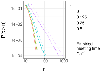
(b)

Figure 2: Beta-Bernoulli model. Left: Plots of the prior and posterior distribution of paramter $\beta$. Right: Plots of the tail probability $\mathds{P}(\tau>n)$ for a range of values of $\epsilon$. Dotted lines show bounding polynomials of the form $Cn^{-\kappa^{\prime}}$ for each of the values of $\epsilon$.

4 Experiments in state space models

State space models are a popular class of time series models. These latent variable models are defined by an unobserved Markov process $(X_{t})_{t\geq 0}$ and an observation process $(Y_{t})_{t\geq 1}$ where the observations are conditionally independent given $(X_{t})_{t\geq 0}$ with

$$X_{0}\sim\mu_{\theta}(\cdot),\quad\quad X_{t}|\{X_{t-1}=x\}\sim f_{\theta}(\cdot|x),\quad\quad Y_{t}|\{X_{t}=x\}\sim g_{\theta}(\cdot|x),$$ (16)

where $\theta$ parameterizes the distributions $\mu_{\theta}$, $f_{\theta}$ and $g_{\theta}$ (termed the ‘initial’, ‘transition’ and ‘observation’ distribution respectively). Given a realization of the observations $Y_{1:T}=y_{1:T},$ we are interested in performing Bayesian inference on the parameter $\theta$ to which we assign a prior density $p(\theta)$. The posterior density of interest is thus $\pi\left(\theta\right)\propto p(\theta)p(y_{1:T}|\theta)$ where the likelihood $p(y_{1:T}|\theta)=\int\mu_{\theta}(dx_{0})\prod_{t=1}^{T}f_{\theta}(dx_{t}|x_{t-1})g_{\theta}(y_{t}|x_{t})$ is usually intractable. It is possible to obtain a non-negative unbiased estimator $\widehat{p}(y|\theta,u)$ of $p(y|\theta)$ using particle filtering where here $u$ represents all the random variables simulated during the run of a particle filter. The resulting pseudo-marginal algorithm is known as the particle marginal MH algorithm (PMMH) (Andrieu et al., 2010). This algorithm can also be easily modified to perform unbiased smoothing for state inference and is an alternative to existing methods in Jacob et al. (2019). Guidelines on the selection of the number of particle in this context are provided in Middleton et al. (2019). For state-space models, it is unfortunately extremely difficult to check that Assumptions 6 and 7 are verified.

4.1 Linear Gaussian state space model

The following experiments explore the proposed unbiased estimators in a linear Gaussian state space model where the likelihood can be evaluated exactly. This allows a comparison between the pseudo-marginal kernels, that use bootstrap particle filters (Gordon et al., 1993) with $N$ particles to estimate the likelihood, and the ideal kernels that use exact likelihood evaluations obtained with Kalman filters. We assume $X_{0}\sim\mathcal{N}(0,1),\leavevmode\nobreak\ X_{t}|\{X_{t-1}=x\}\sim\mathcal{N}(ax,\sigma_{X}^{2})$ and $Y_{t}|\{X_{t}=x\}\sim\mathcal{N}(x,1)$ where $a$ and $\sigma_{X}$ are assigned prior distributions, $a\sim\mathcal{U}[0,1]$ and $\sigma_{X}\sim\Gamma(2,2)$.

4.1.1 Effect of the number of particles

A dataset of $T=100$ observations was generated from the model with parameters $a=0.5$ and $\sigma_{X}=1$. We study how the meeting times and the efficiency vary as a function of $N$, the number of particles. We set the initial distribution to $\mathcal{U}[0,1]$ over $a$ and $\mathcal{U}[0,5]$ over $\sigma_{X}$, and the proposal covariance of the Normal random walk proposals to $0.2^{2}I$, corresponding to acceptance rate for the exact algorithm of approximately 36.6%. In the following we consider a grid of values for the number of particles, varying $N$ between 50 and 250.

We estimate large quantiles of the distribution of the meeting time over 20,000 repetitions of coupled PMMH, with the results shown in Figure 3a. As expected, increasing $N$ generally reduces the meeting time at the cost of more computation per iteration.

We examine $\text{IF}[H_{k:m}]$, as defined in section 1.5, for the proposed unbiased estimators with $h:x\mapsto x_{1}+x_{2}+x_{1}^{2}+x_{2}^{2}$, for each of these values of $N$ and consider three cases for $k$ and $m$, in particular

$$(k,m)\in\{(250,500),(250,1000),(750,1000)\}$$

corresponding to the following: (1) a smaller value of $m-k$, (2) a larger value of $m-k$ and (3) a smaller value of $m-k$ with a more conservative choice of $k$. Estimates of $\text{IF}[H_{k:m}]$ were obtained using 20,000 repetitions of coupled PMMH where for each value of $(k,m)$ estimators were obtained using a single realisation of the largest value of $m=1,000$ using 30 cores of an Intel Xeon CPU E5-4657L 2.40GHz, taking approximately 60 hours in total.

The results are plotted in Figure 3b where we plot also the inefficiency of estimators obtained using coupled Metropolis-Hastings (horizontal line) for $(k,m)$ as in case (2). We see first of all that the inefficiency is reduced by increasing $N$ in all cases, and that the inefficiency of estimators obtained using coupled PMMH asymptotes over this range of $N$ towards the inefficiency of estimators obtained using coupled Metropolis-Hastings for $N$ increasing. We also see that for case (3) that the larger value of $k$ can ameliorate the efficiency of the estimators for small numbers of particles.

We also examine the inefficiency weighted by the cost of obtaining each estimator, i.e. $N\text{IF}[H_{k:m}]$, and compare this to the inefficiency of the serial algorithm using $NV_{\text{as}}$, with the notation of Section 1. Here, $V_{\text{as}}$ was estimated using the spectrum0.ar function in R’s CODA package (Plummer et al., 2006), averaging over 10 estimators obtained through running the serial algorithm for 500,000 iterations and discarding the first 10% as burn-in. Figure 4 shows the results of this procedure, showing $\pm 2$ sample standard errors for the inefficiency estimates. Figure 4a demonstrates that despite the lower cost of obtaining unbiased estimators for lower values of $N$, the initial decline in inefficiency is still significant. In Figure 4b we show the same results though with a focus around the optimum inefficiency. Here, we see that the optimum is attained at $N=100$ with value $NV_{\text{as}}=640$ for the serial algorithm and at $N=150$ with $N\text{IF}[H_{k:m}]=980$ for case (2). Therefore, we see that the increase in inefficiency is estimated to be under 55% relative to a well-tuned serial algorithm for the values considered. Indeed, for this particular batch of $N=150$ and $m=1,000$, the parallel execution time to obtain the estimators $H_{k:m}$ on the stated machine was under 14 hours, which we compare to approximately 12 days of serial execution time if performed all on a single core (the mean time to obtain an estimator was 53 seconds) or 8 days after accounting for the increase in inefficiency of 55%.

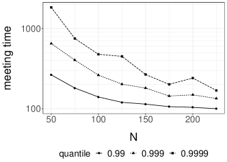
(a)

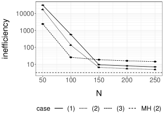
(b)

Figure 3: Coupled PMMH meeting times and inefficiency of estimators for a linear Gaussian state space model with $T=100$ observations and over a range of particles, $N$. Left: estimates of the quantiles of the meeting times. Right: inefficiencies for serial PMMH as a function of $N$, compared to the inefficiency of unbiased estimators obtained using coupled MH.

(a)

(b)

Figure 4: Inefficiencies weighted by $N$ for a linear Gaussian state space model, comparing directly the inefficiency of estimators obtained using the serial algorithm to those obtained using coupled PMMH. Left: inefficiencies weighted by $N$. Right: inefficiencies weighted by $N$ close to their optima.

4.1.2 Effect of the time horizon

We investigate the distribution of meeting times as a function of $T$, with $N$ scaling linearly with $T$. Such a scaling is motivated through the guarantee that the variance of the log-likelihood estimates obtained at each iteration are asymptotically constant (Bérard et al., 2014; Deligiannidis et al., 2018; Schmon et al., 2020). For the model as before, we consider a grid of $T\in\{100,...,1000\}$, using a single realisation of the data. Throughout the following, we fix the proposal covariance to be $\frac{2^{2}}{T}I$, coinciding with the proposal covariance in 4.1.1 for $T=100$, providing an acceptable acceptance rate for the exact algorithm and where $1/T$ is motivated as a result of the variance of the posterior contracting at a rate proportional to $1/T$.

We consider two cases. Firstly, we examine how the distribution of meeting time changes for a fixed initial distribution (the distribution used previously of $\mathcal{U}[0,1]$ over $a$ and $\mathcal{U}[0,5]$ over $\sigma_{X}$); we refer to this as Scaling 1. Secondly, for Scaling 2, we examine how the distribution of meeting times changes if we also scale the initial distribution by setting $\pi_{0}=\mathcal{N}(\mu^{*},\frac{50}{T}I)$, truncated to ensure it is dominated by the prior and where $\mu^{*}$ denotes the true parameter values.

In both cases we compare the distribution of meeting times for $N=T$ with the distribution of meeting times for the exact algorithm (i.e. $\bar{P}$ as in Algorithm 2) with likelihood evaluations performed using the Kalman filter. Figure 5a and 5b show estimates of the $80^{th}$ and $99^{th}$ percentile over 1,000 repetitions for Scaling 1 and Scaling 2 respectively. Firstly, it can be seen that in all cases the meeting times for coupled PMMH are higher than the meeting times for coupled MH. Furthermore the smaller difference between the $80^{th}$ percentiles, compared to the difference between the $99^{th}$ percentiles, reflects a heavier tail of the distribution of the meeting time in the case of PMMH. Finally, it can be seen that out of the two scalings Scaling 2 appears to stabilise for larger values of $T$ whereas Scaling 1 exhibits an increase with $T$.

(a)

      

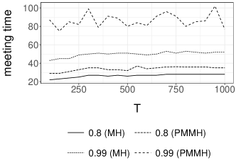
(b)

Figure 5: Scaling quantiles of meeting times with $T$ over 1,000 repetitions. Left: fixing the initial distribution and scaling the proposals (Scaling 1). Right: scaling both the proposals and the initial distribution (Scaling 2).

4.2 Neuroscience experiment

We apply the proposed methodology to a neuroscience experiment described in Temereanca et al. (2008). The same data and model were used to illustrate the controlled Sequential Monte Carlo (cSMC) algorithm in Heng et al. (2020).

4.2.1 Model, data and target distribution

The model aims at capturing the activation of neurons of rats as their whiskers are being moved with a periodic stimulus. The experiment involves $M=50$ repeated experiments, and $T=3000$ measurements (one per millisecond) during each experiment. The activation of a neuron is recorded as a binary variable for each time and each experiment. These activation variables are then aggregated by summing over the $M$ experiments at each time step, yielding a series of variables $Y_{t}$ taking values between $0$ and $M$; see Zhang et al. (2018) for an alternative analysis that avoids aggregating over experiments. Letting $\text{Bin}(\cdot;n,p)$ denote the binomial distribution for $n$ trials with success probability $p$, the model for neuron activation is given by $X_{0}\sim\mathcal{N}(0,1)$ and, for $t\geq 1$,

$$X_{t}|\{X_{t-1}=x\} \sim\mathcal{N}(\cdot;ax,\sigma_{X}^{2}),\quad Y_{t}|\{X_{t}=x\}\sim\text{Bin}(\cdot;M,s(x))$$

where $s(x):=(1+\exp(-s))^{-1}$. We focus on the task of estimating $(a,\sigma_{X}^{2})$ from the data using the proposed method. Following Heng et al. (2020) we specify a uniform prior on $[0,1]$ for $a$ and an inverse-Gamma prior on $\sigma_{X}^{2}$ with parameters $(1,0.1)$, where the probability density function of an inverse-Gamma with parameters $(a,b)$ is $x\,\mapsto\Gamma(a)^{-1}b^{a}x^{-a-1}\exp(-b/x)$. The PMMH kernels employed below use a Gaussian random walk proposal. The likelihood is estimated with cSMC with $N=128$ particles and $3$ iterations, where the exact specification is taken from the appendix of Heng et al. (2020). Such cSMC runs take approximately one second, on a 2015 desktop computer and a simple R implementation. Figure 6 presents the time series of observations (6a) and the estimated log-posterior density (6b), obtained on a $500\times 500$ grid of parameter values, and one cSMC likelihood estimate per parameter value. In Figure 6b, the upper right corner presents small black circles, generated by the contour plot function, which indicate high variance in the likelihood estimators for these parameters. Thus we expect PMMH chains to have a lower acceptance rate in that part of the space. On the other hand, the maximum likelihood estimate (MLE) is indicated by a black dot on the bottom right corner. The variance of the log-likelihood estimators is of the order of $0.2$ around the MLE, so that PMMH chains are expected to perform well there, as was observed in Heng et al. (2020) where the chains were initialized close to the MLE.

(a)

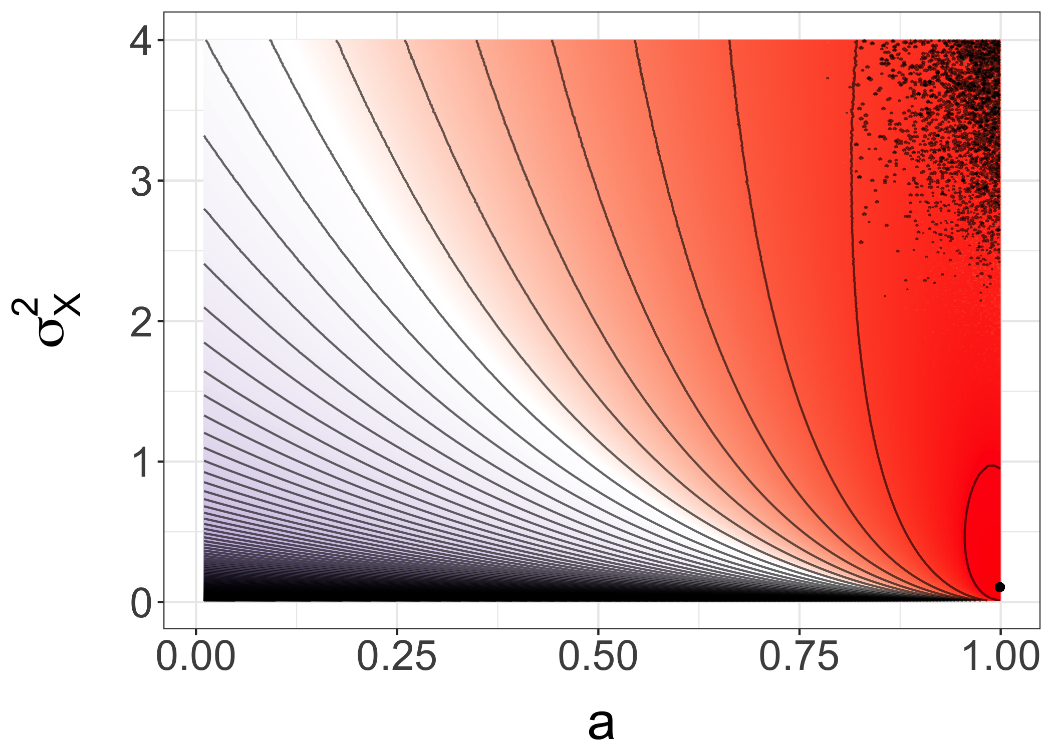
(b)

Figure 6: Left: counts of neuron activation in $50$ experiments, over a duration of three seconds. Right: estimated log-posterior density in the neuroscience experiment of Section 4.2.

4.2.2 Standard deviation of the proposal

Here, we initialize the chains from a uniform distribution on $[0,1]^{2}$, and we investigate two choices of standard deviation for the random walk proposals: the one used in Heng et al. (2020), that is $0.002$ for $a$ and $0.01$ for $\sigma_{X}^{2}$, and another choice equal to $0.01$ for $a$ and $0.05$ for $\sigma_{X}^{2}$, i.e. five times larger. For each choice, we can run pairs of chains until they meet and record the meeting time; we can do so on $P$ processors in parallel (e.g. hundreds), and for a certain duration (e.g. a few hours). Thus the number of meeting times produced by each processor is a random variable. Following Glynn and Heidelberger (1990), if no meeting time was produced by a processor within the time budget, the computation continues until one meeting time is produced, otherwise on-going calculations are interrupted when the budget is reached. This allows unbiased estimation of functions of the meeting time on each processor via Corollary 7 of Glynn and Heidelberger (1990), and then we can average across processors. In particular we use this strategy to produce all histograms in the present section, as in Figure 7.

We observe that the meeting times are significatively larger when using the smaller standard deviation (7a), with a maximum value of $21,570$ over $1565$ realizations. With the larger choice of standard deviation (7b), we observe shorter meeting times, with a maximum of $928$ over $5572$ realizations. This suggests that the values of $k$ and $m$ should be chosen very differently in both cases.

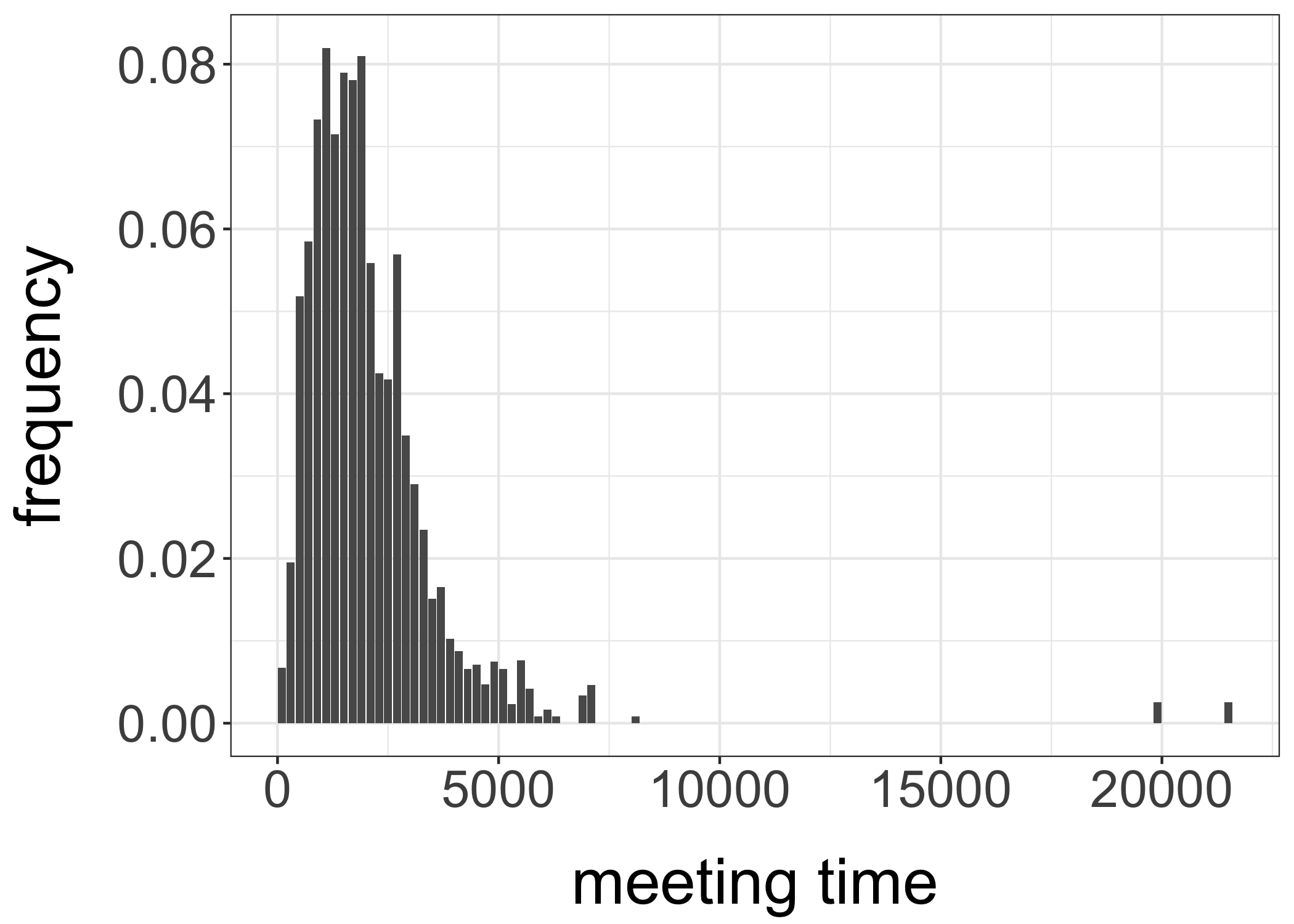
(a)

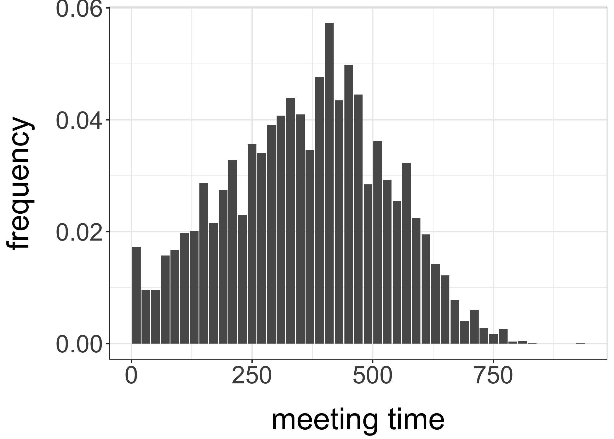
(b)

Figure 7: Histograms of meeting times associated with coupled PMMH chains, obtained with a standard deviation of the random walk proposal of $0.002$ for $a$ and $0.01$ for $\sigma_{X}^{2}$ on the left, and with a larger standard deviation ($0.01$ on $a$ and $0.05$ on $\sigma_{X}^{2}$) on the right. In both cases, the likelihood was estimated with controlled SMC, with $N=128$ particles, $I=3$ iterations, in the neuroscience model of Section 4.2.

To explain this difference we investigate the realization of the coupled chains that led to the largest meeting time of $21,570$, in Figure 8. Figure 8a presents the trajectories of two chains overlaid with contours of the target density function. The chains seem to follow approximately the gradient of the density. Given the shape of this density, it means that small starting values for component $a$ result in the chains going to the region of high variance of the likelihood estimator, in the top right corner of the plot. The marginal trace plots of one of the two chains are shown in 8b. From the trace plots we see that most of the $21,570$ iterations have been spent in that top right corner, where the chain got stuck, approximately between iterations $2,000$ and $20,000$. The overall acceptance rate is of $6\%$ for that chain, compared to $39\%$ for the other chain shown in 8a Therefore the use of a larger proposal standard deviation seems to have a very noticeable effect here on the ability of the Markov chain to escape a region of high variance of the likelihood estimator.

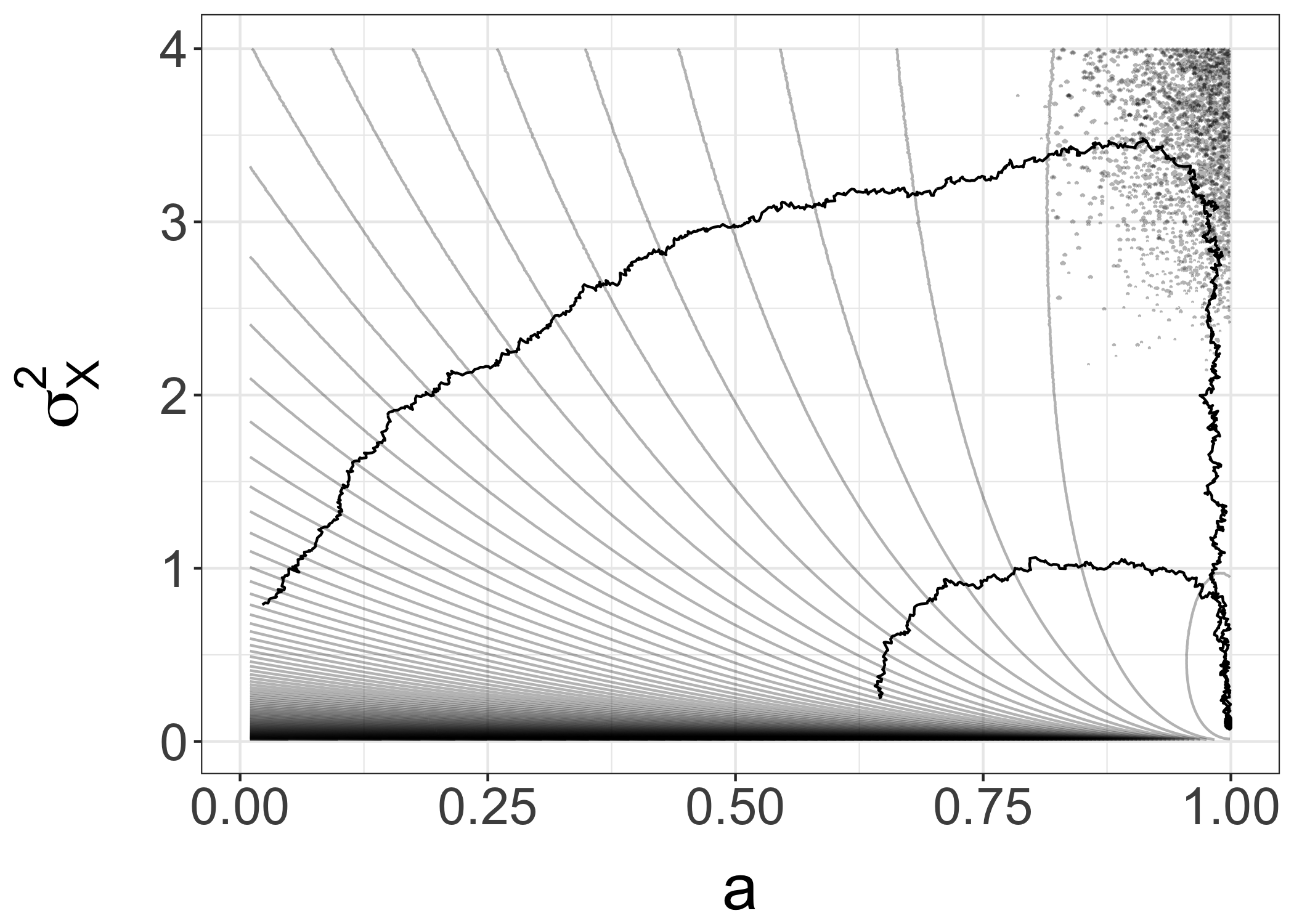
(a)

(b)

Figure 8: Traces of the chains corresponding to the largest observed meeting time ($21,570$) obtained with a small standard deviation of the random walk proposal ($0.002$ for $a$ and $0.01$ for $\sigma_{X}^{2}$), in form of a two-dimensional trajectory on the left, and trace plots of one of the two chains on the right. The likelihood is estimated with controlled SMC, with $N=128$ particles, $I=3$ iterations, in the neuroscience experiment of Section 4.2.

4.2.3 Comparison with PMMH using bootstrap particle filters

We use the larger choice of standard deviation ($0.01$ on $a$ and $0.05$ on $\sigma_{X}^{2}$) hereafter, and compare meeting times obtained with cSMC with those obtained with bootstrap particle filters, with $N=4,096$ particles. This number is chosen so that the compute times are comparable. Over 23 hours of compute time, the number of meeting times obtained per processor varied between $4$ and $35$, and a total of $7,776$ meeting times were obtained from $400$ processors. The meeting times are plotted against the duration it took to produce them in Figure 9a. The compute time associated with meeting times is not only proportional to the meeting times themselves, but also varies across processors. This is partly due to hardware heterogeneity across processors, and to concurrent tasks being executed on the cluster during our experiments. The histogram in Figure 9b shows that meeting times are larger, and heavier tailed, than when using cSMC (see Figure 7b). The maximum observed value is $9,371$. From these plots, we see that to produce unbiased estimators $H_{k:m}$ using BPF with a similar variance as when using cSMC, we would have to choose larger values of $k$ and $m$, and thus the cost per estimator would likely be higher.

(a)

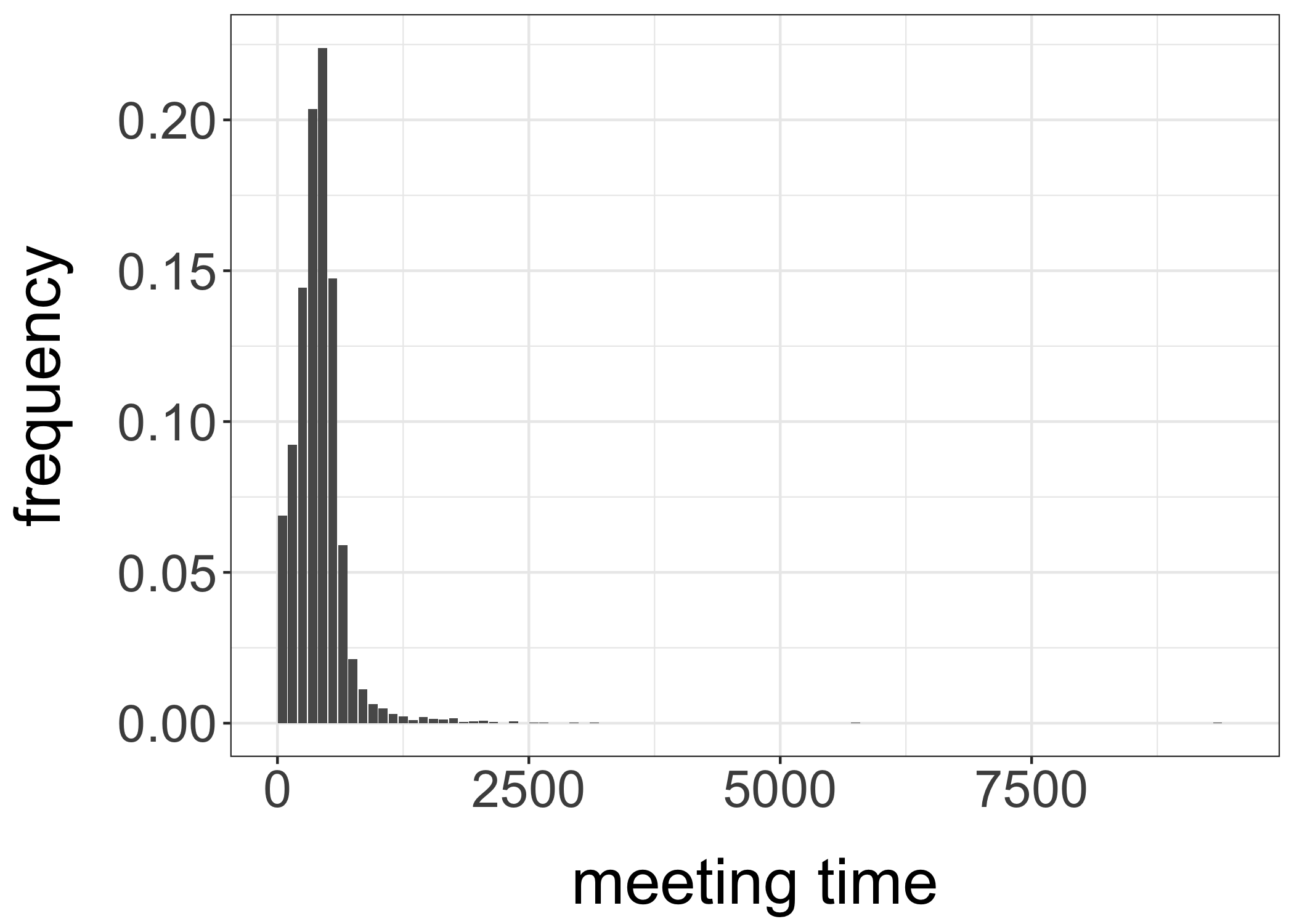
(b)

Figure 9: Left: duration (in hours) versus meeting times, using BPF with $N=4,096$ particles. Each color corresponds to a different processor. Right: estimated histogram of the meeting times, in the neuroscience experiment of Section 4.2.

4.2.4 Efficiency compared to the serial algorithm

Using cSMC and the larger choice of standard deviation for the proposal, we produce unbiased estimators $H_{k:m}$ with $k=1,000$ and $m=10,000$. We run $100$ processors for a time budget of $23$ hours, and each processor produced between $2$ and $9$ estimators, for a total of $578$ estimators. The generation of samples for each processor is represented chronologically in Figure 10a. The variation among durations is due to the randomness of meeting times and also to external factors such as concurrent tasks being executed on the cluster. We produce histograms of the posterior marginals in Figure 10b, with the result from a long run of PMMH with cSMC ($250,000$ iterations) overlaid in red lines.

(a)

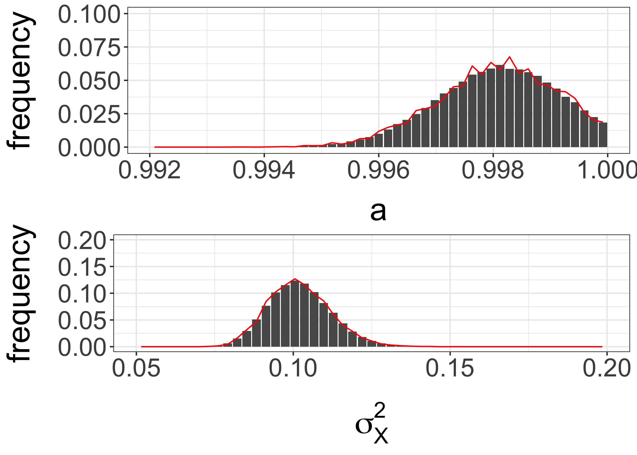
(b)

Figure 10: Left: start and end time for the calculation of unbiased estimators on $100$ parallel processors, for a budget of $23$ hours (dashed line), with cSMC, $N=128$ particles, $I=3$ iterations and $k=1,000$, $m=10,000$. Right: estimated histograms of both parameters $a$ and $\sigma_{X}^{2}$; the red lines correspond to estimates obtained with $250,000$ iterations of PMMH and discarding the first $10,000$ as burn-in; this is for the neuroscience experiment of Section 4.2.

We compute the loss of efficiency incurred by debiasing the PMMH chain with the proposed estimators. We consider the test function $h:x\mapsto x_{1}+x_{2}+x_{1}^{2}+x_{2}^{2}$. Along the PMMH chain of length $n_{\text{mcmc}}=250,000$, after a burn-in of $n_{\text{burnin}}=10,000$ steps, and using the spectrum0 function of the CODA package, we find the asymptotic variance associated with $h$ to be $V_{\text{as}}=7.53\cdot 10^{-3}$. If we measure computing cost in terms of MCMC iterations, we obtain an inefficiency of $n_{\text{mcmc}}\times V_{\text{as}}/(n_{\text{mcmc}}-n_{\text{burnin}})\approx 7.84\cdot 10^{-3}$. With the unbiased estimators $H_{k:m}$, if the cost of an estimator is $2(\tau-1)+\max(1,m+1-\tau)$, then the average cost per processor is $59,860$. The empirical variance of the unbiased estimators obtained per processor is equal to $1.4\cdot 10^{-7}$, thus we obtain an inefficiency of $59860\times 1.4\cdot 10^{-7}\approx 8.4\cdot 10^{-3}$. This inefficiency is slightly above $7.84\cdot 10^{-3}$.

Next, we parameterize cost in terms of time (in seconds) instead of number of MCMC steps. This accounts for the fact that running jobs on a cluster involve heterogeneous hardware and concurrent tasks. The serial PMMH algorithm was run on a desktop computer for $169,952$ seconds and thus the inefficiency might be measured as $169,952\times V_{\text{as}}/(n_{\text{mcmc}}-n_{\text{burnin}})\approx 5.3\cdot 10^{-3}$. Note that each iteration took less than a second on average, because parameter values proposed outside of the support of the prior were rejected before running a particle filter; on the other hand the cost of a cSMC run is above one second on average. For the proposed estimators, the budget was set to $23$ hours and we obtained a variance across processors of $1.4\cdot 10^{-7}$; thus we can compute the inefficiency as $1.16\cdot 10^{-2}$, which is approximately twice the inefficiency of the serial algorithm.

5 Methodological extensions

The following provides two further examples of coupled MCMC algorithms to perform inference when the likelihood function is intractable. The associated estimators are not covered by our theoretical results.

5.1 Block pseudo-marginal method

Block pseudo-marginal methods have demonstrated significant computational savings for Bayesian inference for random effects models over standard pseudo-marginal methods (Tran et al., 2016). Such methods proceed through introducing strong positive correlation between the current likelihood estimate $\hat{p}(y|\theta)$ and the likelihood estimate of the proposed parameter $\hat{p}(y|\theta^{\prime})$ through only modifying a subset of the auxiliary variables used to obtain the likelihood estimate at each iteration. We here demonstrate the computational benefits of such a scheme in obtaining unbiased estimators of posterior expectations.

We focus here on random effects models, as defined in section 3.2.1. We recall that the likelihood estimate is given by $\hat{p}(y|\theta,U)=\prod_{t=1}^{T}\hat{p}(y_{t}|\theta,U_{t})$, where $\{\hat{p}(y_{t}|\theta,U{}_{t})\}_{t=1,...,T}$ are $T$ independent non-negative unbiased likelihood estimates of $\{p(y_{t}|\theta)\}_{t=1,...,T}$ when $U_{t}\sim m_{t}(\cdot)$. In the following, we provide a minor modification of the blocking strategy proposed in Tran et al. (2016), where instead of jointly proposing a new parameter and a single block of auxiliary random variables, a parameter update is performed, followed by sequentially iterating through the auxiliary random variables used to construct the likelihood estimate of observation $t$. For each data $t$, new values are proposed according to $U_{t}^{\prime}\sim m_{t}(\cdot)$ and accepted with probability

$$\alpha_{\mathrm{BPM},t}\left\{\widehat{p}(y_{t}\mid\theta,U_{t}),\hat{p}(y_{t}|\theta,U^{\prime}_{t})\right\}=\min\left\{1,\frac{\hat{p}(y_{t}|\theta,U^{\prime}_{t})}{\hat{p}(y_{t}|\theta,U{}_{t})}\right\}.$$ (17)

As remarked in Tran et al. (2016), such blocking strategies are generally not applicable to particle filter inference in state space models, whereby likelihood estimates for observation $t$ typically depend on all auxiliary random variables generated up to and including $t$. We provide pseudo-code for the proposed blocking strategy in Algorithm 4. We denote by $U_{t,n}$ the set of auxiliary variables $U_{t}$ at iteration $n$,

Algorithm 4 Sampling from the block pseudo-marginal kernel given $\left(\theta_{n-1},(U_{t,n-1})_{{}_{t\geq 1}}\right)$

1. Sample $\theta^{\prime}\sim q\left(\cdot|\theta_{n-1}\right)$ and compute $\widehat{p}(y_{t}\mid\theta^{\prime},U_{t,n-1})$ for $t=1,...,T$.

2. With probability $\alpha_{\mathrm{PM}}\left\{(\theta_{n-1},\prod_{t=1}^{T}\widehat{p}(y_{t}\mid\theta_{n-1},U_{t,n-1})),(\theta^{\prime},\prod_{t=1}^{T}\widehat{p}(y_{t}\mid\theta^{\prime},U_{t,n-1}))\right\}$, set $\theta_{n}=\theta^{\prime}$. Otherwise, set $\theta_{n}=\theta_{n-1}$.

3. For $t=1,...,T$

   1. Sample $U^{\prime}_{t}\sim m{}_{t}\left(\cdot\right)$.

   2. With probability $\alpha_{\mathrm{BPM,t}}\left\{\widehat{p}(y_{t}\mid\theta_{n},U_{t,n-1}),\widehat{p}(y_{t}\mid\theta_{n},U^{\prime}_{t})\right\}$, set $U_{t,n}=U^{\prime}_{t}$. Otherwise, set $U_{t,n}=U_{t,n-1}$.

5.1.1 Coupled block pseudo-marginal method

An algorithm to couple two block pseudo-marginal algorithms to construct unbiased estimators $H_{k:m}$ is provided in Algorithm 5. Denoting the two states of the chains at step $n\geq 1$ by $(\theta_{n},(U_{t,n})_{{}_{t\geq 1}})$ and $(\tilde{\theta}{}_{n-1},(\widetilde{U}_{t,n-1})_{{}_{t\geq 1}})$, Algorithm 5 describes how to obtain $(\theta_{n+1},(U_{t,n+1})_{{}_{t\geq 1}})$ and $(\tilde{\theta}{}_{n},(\widetilde{U}_{t,n})_{{}_{t\geq 1}})$; thus it describes a kernel $\bar{P}$.

Algorithm 5 Sampling from the coupled block pseudo-marginal kernel given $(\theta_{n},(U_{t,n})_{{}_{t\geq 1}},\tilde{\theta}{}_{n-1},(\widetilde{U}_{t,n-1})_{{}_{t\geq 1}})$

1. Sample $(\theta^{\prime},\tilde{\theta}^{\prime})$ from the maximal coupling of $q\left(\cdot|\theta_{n}\right)$ and $q(\cdot|\tilde{\theta}{}_{n-1})$.

2. Compute $\widehat{p}(y_{t}\mid\theta^{\prime},U_{t,n})$ and $\widehat{p}(y_{t}\mid\tilde{\theta}^{\prime},\widetilde{U}_{t,n-1})$ for $t=1,...,T$.

3. Sample $\mathit{\mathfrak{u}}\sim\mathcal{U}\left[0,1\right]$.

4. If $\mathit{\mathfrak{u}}<\alpha_{\mathrm{PM}}\left\{\left(\theta_{n},\prod_{t=1}^{T}\widehat{p}(y_{t}\mid\theta_{n},U_{t,n})\right),(\theta^{\prime},\prod_{t=1}^{T}\widehat{p}(y_{t}\mid\theta^{\prime},U_{t,n}))\right\}$ then set $\theta_{n+1}=\theta^{\prime}$. Otherwise, set $\theta_{n+1}=\theta_{n}$.

5. If $\mathit{\mathfrak{u}}<\alpha_{\mathrm{PM}}\left\{(\tilde{\theta}_{n-1},\prod_{t=1}^{T}\widehat{p}(y_{t}\mid\tilde{\theta}{}_{n-1},\widetilde{U}_{t,n-1})),(\tilde{\theta}^{\prime},\prod_{t=1}^{T}\hat{p}(y_{t}|\tilde{\theta}^{\prime},\widetilde{U}_{t,n-1}))\right\}$ then set $\tilde{\theta}_{n}=\tilde{\theta}^{\prime}$. Otherwise, set $\tilde{\theta}_{n}=\tilde{\theta}_{n-1}$.

6. For $t=1,...,T$

   1. Sample $U^{\prime}_{t}\sim m_{t}(\cdot)$.

   2. Sample $\mathit{\mathfrak{u}}\sim\mathcal{U}\left[0,1\right]$.

   3. If $\mathit{\mathfrak{u}}<\alpha_{\mathrm{BPM,t}}\left\{\widehat{p}(y_{t}\mid\theta_{n+1},U_{t,n}),\widehat{p}(y_{t}\mid\theta_{n+1},U^{\prime}_{t})\right\}$ then set $U_{t,n+1}=U^{\prime}_{t}$. Otherwise, set $U_{t,n+1}=U{}_{t,n}$.

   4. If $\mathit{\mathfrak{u}}<\alpha_{\mathrm{BPM,t}}\left\{\widehat{p}(y_{t}\mid\tilde{\theta}_{n},\tilde{U}_{t,n-1}),\widehat{p}(y_{t}\mid\tilde{\theta}_{n},U^{\prime}_{t})\right\}$ then set $\widetilde{U}_{t,n}=U^{\prime}_{t}$. Otherwise, set $\widetilde{U}_{t,n}=\widetilde{U}_{t,n-1}$.

5.1.2 Bayesian multivariate probit regression

The following demonstrates the proposed algorithm for a latent variable model applied to polling data and explores the possible gains when compared to the unbiased estimators obtained using the coupled pseudo-marginal algorithm. The data consists of polling data collected between February 2014 and June 2017 as part of the British Election Study (Fieldhouse et al., 2018). We use a multivariate probit model, which for $i\in\{1,..,T\}$ and $j\in\{1,2,3\}$ can be expressed as $X_{ij}=\beta^{\prime}\zeta_{ij}+\epsilon_{ij}$ and $Y_{ij}=\mathds{1}[X_{ij}>0]$ for observed binary response $Y_{ij}$, latent state $X_{ij}$ and where $i$ indexes the $i^{th}$ participant, $j$ indexes the $j^{th}$ wave of questions, $\beta$ is a vector of regression coefficients (including an intercept) and $\zeta_{ij}$ is a vector of independent variables.

We use a random sample of $T=2,000$ participants over three waves (one a year) in the run up to the United Kingdom’s European Union membership referendum on $23^{rd}$ June 2016, regressing the binary outcome asking participants how they would vote in an EU referendum against how they perceive the general economic situation in the UK has changed over the previous 12 months (graded 1-5, with 1=‘Got a lot worse’, 5=‘Got a lot better’). A detailed description of the data is provided in Appendix A.6.

We allow for correlations between waves through modelling the perturbations $(\epsilon_{i1},\epsilon_{i2},\epsilon_{i3})\sim\mathcal{N}(0,\Sigma_{\rho})$ with a generic correlation matrix $\Sigma_{\rho}$. In total, we have five unknown parameters $\theta=(\beta_{1},\beta_{2},\rho_{2,1},\rho_{3,1},\rho_{3,2})$, with $\beta_{1}$ denoting a regressor coefficient, $\beta_{2}$ a constant offset and $\rho_{s,t}$ element $(s,t)$ of $\Sigma_{\rho}$. We place independent priors on each parameter with $\beta_{1},\beta_{2}\stackrel{{\scriptstyle i.i.d.}}{{\sim}}\mathcal{N}(0,10^{2})$ and $\rho_{s,t}\stackrel{{\scriptstyle i.i.d.}}{{\sim}}\mathcal{U}[-1,1]$, where we additionally truncate the prior on $\Sigma_{\rho}$ to ensure support only on the manifold of positive definite matrices.

Inference

For each observation $y_{i}:=(y_{i1},y_{i2},y_{i3})$, we obtain unbiased estimates of the likelihood of $\theta$ using the sequential importance sampling algorithm of Geweke, Hajivassiliou and Keane; see, e.g., Train (2009, 5.6.3) and references therein. We set the initial distribution $\pi_{0}=\mathcal{N}(\hat{\mu},0.01^{2}I)$, supported only on areas of positive mass under the prior (we employ a simple rejection sampling algorithm to sample $\Sigma_{\rho}$ initially) and use a Normal random walk proposal with covariance set to $\frac{2.38^{2}}{5}\hat{\Sigma}$, see Roberts et al. (1997), following where $\hat{\mu}$ and $\hat{\Sigma}$ are an empirical estimate of the posterior mean and covariance on a preliminary run of 10,000 iterations of block pseudo-marginal with $N=40$ discarding the first 10% as burn-in.

We compare coupled block pseudo-marginal with coupled pseudo-marginal. We examine values of $N$ for the latter that are close to the optimal value of $N$ for the serial algorithm, estimated through ensuring the variance of the log-likelihood estimates is between 1 and 2, as per the guidance in Doucet et al. (2015). In this case we consider $N\in\{600,700,800\}$, providing a corresponding variance of the log-likelihood estimates given by $\{1.67,1.40,1.25\}$ (estimated using 10,000 likelihood estimates at $\hat{\mu}$). For the block pseudo-marginal algorithm we consider $N\in\{5,10,20\}$.

Meeting times

Both algorithms were run continuously until coupling for half an hour each on a 48 CPU Intel Xeon 2.4Ghz E5-4657L server, with the number of estimators produced for block pseudo-marginal varying between 2,000 and 4,000 for the values of $N$ considered and between 160 and 180 for the pseudo-marginal. The meeting times are plotted in Figure 11a, where it can be seen that despite the lower cost of the block pseudo-marginal algorithm the absolute values of the meeting times are comparable across algorithms.

Accordingly, we also plot the distribution of meeting times accounting for the cost of running each algorithm, i.e. $N\tau$ for the pseudo-marginal algorithm and $2N\tau$ for the block pseudo-marginal algorithm. The additional factor of $2$ for the latter can be seen as an upper bound on the additional computational cost of the block pseudo-marginal algorithm, assuming twice the density evaluations per complete iteration and less than twice the number of pseudo-random numbers generated. Figure 11b shows the results of this additional cost-weighting where it can be seen that meeting times are between 1 and 2 orders of magnitude larger for the pseudo-marginal over the block pseudo-marginal algorithm.

(a)

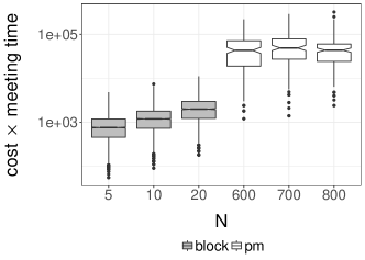
(b)

Figure 11: Meeting times for coupled block pseudo-marginal and coupled pseudo-marginal algorithms. Left: raw meeting times for the two algorithms. Right: meeting times weighted by cost for the two algorithms, i.e. $\tau N$ for coupled pseudo-marginal and $2\tau N$ for coupled block pseudo-marginal.

Variance of estimators

We estimate the increase in inefficiency of the coupled over the serial algorithm for $N=10$, $k=500$ and $m=5,000$; the choice of $k$ is guided by the meeting times in Figure 11a. Running coupled block pseudo-marginal 200 times, we estimate the variance using the test function $h:x\mapsto\sum_{i}(x_{i}+x_{i}^{2})$ to be $1.05\cdot 10^{-5}$. Estimating the cost of $2(\tau-1)+\max(1,m+1-\tau)$ to be 5121, implies an inefficiency of $5.36\cdot 10^{-2}$. In comparison, we estimate the inefficiency of the serial algorithm using spectrum0.ar as before on runs of length 125,000 (discarding 10% as burn-in and averaging over 20 estimators) to be $n_{\text{mcmc}}\times V_{as}/(n_{\text{mcmc}}-n_{\text{burnin}})=4.82\cdot 10^{-2}$ suggesting an increase in inefficiency of $11\%$ for the unbiased estimators.

Finally, we compare the inefficiency of unbiased estimators generated with coupled block pseudo-marginal kernels with those produced using standard coupled pseudo-marginal kernels with $N_{\text{PM}}=700$ particles. For coupled pseudo-marginal, the variance of the unbiased estimator was estimated to be $1.53\cdot 10^{-5}$ and the expected cost was estimated to be $5147$, implying an inefficiency of $7.86\cdot 10^{-2}$. As a result we estimate the improvement of inefficiency for the coupled block pseudo-marginal by $\frac{N_{\text{PM}}}{2N}\times\frac{7.86\cdot 10^{-2}}{5.36\cdot 10^{-2}}$ to be approximately 51 times. Estimation of the asymptotic variance of the serial pseudo-marginal algorithm was computationally infeasible for this many particles, with a single iteration taking on average six seconds on the aforementioned server, hence the choice of $N$ motivated by the guidance in Doucet et al. (2015) instead.

5.2 Exchange algorithm

Problems where the likelihood function is only known only up to a constant of proportionality occur frequently across Bayesian statistics; see, e.g., Park and Haran (2018) for a recent account of current methodology and applications. In this case, posterior distributions $\pi(\theta)\propto p(y|\theta)p\left(\theta\right)$ are given by

$$p(y|\theta)=\frac{f(y|\theta)}{\mathcal{Z}(\theta)},\quad\mathcal{Z}(\theta):=\int f(y|\theta)dy,$$

where $f(y|\theta)$ can be evaluated pointwise but its parameter-dependent normalizing constant $\mathcal{Z}(\theta)$ is intractable. This is a scenario common for undirected graphical models and spatial point processes (Møller et al., 2006; Murray et al., 2006). The exchange method detailed in Algorithm 6 is an MCMC scheme proposed by Murray et al. (2006) to sample such distributions under the assumption that, although $\mathcal{Z}(\theta)$ cannot be evaluated, it is possible to simulate exactly artificial observations from $p(y|\theta)$. This is indeed possible for a large class of spatial point processes as well as the Ising and Potts models using perfect simulation procedures.

Algorithm 6 Sampling from the Exchange kernel given $\theta_{n-1}$

1. Sample $\theta^{\prime}\sim q\left(\cdot|\theta_{n-1}\right)$ and $Y^{\prime}\sim p(\cdot|\theta^{\prime})$.

2. With probability

   $$\alpha_{\mathrm{EX}}\left(\theta_{n-1},\theta^{\prime},Y^{\prime}\right):=\min\left\{1,\frac{f(y|\theta^{\prime})p(\theta^{\prime})f(Y^{\prime}|\theta_{n-1})q\left(\theta_{n-1}|\theta^{\prime}\right)}{f(y|\theta_{n-1})p(\theta_{n-1})f(Y^{\prime}|\theta^{\prime})q(\theta^{\prime}|\theta_{n-1})}\right\},$$ (18)

   set $\theta_{n}=\theta^{\prime}.$ Otherwise, set $\theta_{n}=\theta_{n-1}$.

5.2.1 Coupled exchange algorithm

An algorithm to couple two block pseudo-marginal algorithms to construct unbiased estimators $H_{k:m}$ is provided in Algorithm 7. Denoting the two states of the chains at step $n\geq 1$ by $\theta_{n}$ and $\tilde{\theta}{}_{n-1}$, Algorithm 3 describes how to obtain $\theta_{n+1}$ and $\tilde{\theta}{}_{n}$; thus it describes a kernel $\bar{P}$.

Algorithm 7 Sampling from the coupled Exchange kernel given $(\theta_{n},\tilde{\theta}{}_{n-1})$

1. Sample $\theta^{\prime}$ and $\tilde{\theta}^{\prime}$ from the maximal coupling of $q\left(\cdot|\theta_{n}\right)$ and $q(\cdot|\tilde{\theta}{}_{n-1})$.

2. If the proposals couple, i.e. if $\theta^{\prime}=\tilde{\theta}^{\prime},$ then sample $Y^{\prime}\sim p(\cdot|\theta^{\prime})$ and set $\tilde{Y}^{\prime}=Y^{\prime}$.

3. If the proposals do not couple, sample $Y^{\prime}\sim p(\cdot|\theta^{\prime})$ and $\tilde{Y}^{\prime}\sim p(\cdot|\tilde{\theta}^{\prime})$.

4. Sample $\mathit{\mathfrak{u}}\sim\mathcal{U}\left[0,1\right]$.

5. If $\mathit{\mathfrak{u}}<\alpha_{\mathrm{EX}}\left(\theta_{n},\theta^{\prime},Y^{\prime}\right)$ then set $\theta_{n+1}=\theta^{\prime}.$ Otherwise, set $\theta_{n+1}=\theta_{n}.$

6. If $\mathit{\mathfrak{u}}<\alpha_{\mathrm{EX}}(\tilde{\theta}_{n-1},\tilde{\theta}^{\prime},\tilde{Y}^{\prime})$ then set $\tilde{\theta}_{n}=\tilde{\theta}^{\prime}.$ Otherwise, set $\tilde{\theta}_{n}=\tilde{\theta}_{n-1}.$

5.2.2 High temperature Ising model

We examine the proposed algorithm for inference in a planar lattice Ising model without an external field. The model comprises observations $y_{i}\in\{-1,+1\}$ on a $L\times L$ square lattice such that $p(y|\theta)\propto\exp\left(\beta\sum_{i\sim j}y_{i}y_{j}\right)$ where $i\sim j$ denotes the neighbours $j$ of node $i$ and $\theta=\beta$ denotes the inverse temperature. We restrict interest to high temperature models specifying a prior distribution $\beta\sim\mathcal{U}[0,\beta_{c}]$, with $\beta_{c}=\frac{1}{2}\log(1+\sqrt{2})$ denoting the critical temperature of the Ising model on the infinite lattice (Ullrich, 2013; Onsager, 1944). Here, perfect simulation can be performed using coupling from the past techniques with simple heat bath dynamics developed by Propp and Wilson (1996). We generate observations for $L=80$ and set the proposal covariance to $10^{-4}I$, initialising the chains from the prior.

We obtain estimates of the distribution of meeting times using 1,000 repetitions of coupled exchange, with the results shown in Figure 12a. Based on this, we obtain unbiased estimates of the expectation of $\beta$ under the posterior distribution using $k=100$ and $m=10k$ over 1,000 repetitions. It is noted that the clock time to obtain a single estimator (on the same machine) varies significantly due to the variable computational cost of performing coupling from the past, depending on $\theta$. We plot a histogram of the clock times to obtain each $H_{k:m}$ in Figure 12b.

Based on the heterogeneity of times to produce a single unbiased estimator, we compare the serial inefficiency with the inefficiency of coupled exchange based on the clock time to obtain a certain variance, with the test function $h:x\mapsto x$. We estimate the asymptotic variance with $n_{\text{mcmc}}=200,000$ iterations of the original algorithm (discarding the first 10% as burn-in, and using spectrum0.ar as before) to be $V_{as}\approx 4.22\cdot 10^{-4}$, and the algorithm taking in total $41,095$ seconds. As a result, we estimate the serial inefficiency in terms of clock-time to be $41,095\times V_{\text{as}}/(n_{\text{mcmc}}-n_{\text{burnin}})\approx 9.6\cdot 10^{-5}$. Comparatively, the mean time to return a single estimator $H_{k:m}$ was estimated to be $546$ seconds, with the variance of a single $H_{k:m}$ estimated to be $4.78\cdot 10^{-7}$ providing an estimated inefficiency of $2.6\cdot 10^{-4}$, implying a three-fold increase in inefficiency.

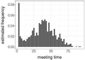
(a)

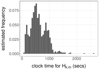
(b)

Figure 12: Coupled exchange algorithm for unbiased Bayesian inference with an $80\times 80$ Ising model. Left: distribution of meeting times (1,000 runs). Right: clock time to obtain 1,000 unbiased estimators.

6 Conclusion

Markov chain Monte Carlo algorithms designed for scenarios where the target density function is intractable can be coupled and utilized in the framework of Glynn and Rhee (2014); Jacob et al. (2020). The validity of the resulting unbiased estimators can be related to polynomial drift conditions on the underlying Markov kernels. These estimators open new ways of using parallel computing hardware to perform numerical integration in such scenarios.

In the context of state space models, in addition to parameter estimation, the proposed coupling strategy for PMMH would additionally provide unbiased estimators with respect to the joint distribution over state and parameters. This would enable unbiased smoothing under parameter uncertainty, instead of fixing the parameters as in Jacob et al. (2019), Lee et al. (2020) and Middleton et al. (2019).

Acknowledgement

The authors are grateful to Jeremy Heng for very helpful discussions. The data of Section 4.2 was kindly shared by Demba Ba. The experiments of that section were performed on the Odyssey cluster supported by the FAS Division of Science, Research Computing Group at Harvard University. Pierre E. Jacob acknowledges support from the National Science Foundation through grant DMS-1712872.

Appendix A Appendix

In the rest of the paper we will often use the symbol $c$ to denote a generic positive constant whose value may vary from line to line.

A.1 Proof of Theorem 1

The following provides a slight relaxation on Assumption 2.2 in Jacob et al. [2020], where geometric conditions were imposed on the tails of the distribution of the meeting time. The following proof considers $H_{0}(Z,\tilde{Z})$ instead of $H_{k:m}$; one can first perform the same reasoning for $H_{k}(Z,\tilde{Z})$ for all $k\geq 0$, and then consider the finite average $(m-k+1)^{-1}\sum_{\ell=k}^{m}H_{\ell}(Z,\tilde{Z})$ to obtain the result for $H_{k:m}$.

By Assumption 2, it follows that $\mathds{E}\left[\tau\right]<\infty$. This implies that the estimator $H_{0}$ can be computed in expected finite time. To show that $H_{0}(Z,\tilde{Z})$ admits a finite variance, we proceed by following Jacob et al. [2020,  Proposition 3.1], adapting the proof under the proposed weaker assumptions. We denote the complete space of random variables with finite second moment by $L_{2}$. We then construct a Cauchy sequence of random variables $H^{n}(Z,\tilde{Z})$ in $L_{2}$ converging to $H_{0}(Z,\tilde{Z})$, where $H^{n}(Z,\tilde{Z}):=\sum_{t=0}^{n}\Delta_{t}$ with $\Delta_{t}=h(Z_{t})-h(\tilde{Z}_{t-1})$ if $t>0$ and $\Delta_{t}=h(Z_{t})$ for $t=0$. As $\mathds{E}\left[\tau\right]<\infty$, we have $\mathds{P}(\tau<\infty)=1$ and $Z_{t}=\tilde{Z}_{t-1}$ for $t>\tau$. This implies that $H^{n}(Z,\tilde{Z})\rightarrow H_{0}(Z,\tilde{Z})$ almost surely. For positive integers $n,n^{\prime}$ we have

$$\mathds{E}\left[\left(H^{n}(Z,\tilde{Z})-H^{n^{\prime}}(Z,\tilde{Z})\right)^{2}\right] =\sum_{s=n+1}^{n^{\prime}}\sum_{t=n+1}^{n^{\prime}}\mathds{E}[\Delta_{s}\Delta_{t}]$$

$$\leq\sum_{s=n+1}^{n^{\prime}}\sum_{t=n+1}^{n^{\prime}}\mathds{E}[\Delta_{s}^{2}]^{1/2}\mathds{E}[\Delta_{t}^{2}]^{1/2}$$

$$=\left(\sum_{t=n+1}^{n^{\prime}}\mathds{E}[\Delta_{t}^{2}]^{1/2}\right)^{2}.$$

We note that $\mathds{E}[\Delta_{t}^{2}]=\mathds{E}[\Delta_{t}^{2}1_{\tau>t}]$. Thus by Holder’s inequality we obtain

$$\mathds{E}[\Delta_{t}^{2}] \leq\mathds{E}\left[\left|\Delta_{t}\right|^{2+\eta}\right]^{\frac{1}{1+\frac{\eta}{2}}}\mathds{E}[1_{\tau>t}]^{\frac{\eta}{2+\eta}}$$

$$\leq c{}^{\frac{1}{1+\frac{\eta}{2}}}\mathds{P}(\tau>t){}^{\frac{\eta}{2+\eta}},$$

where $\mathds{E}[\left|\Delta_{t}\right|^{2+\eta}]<c$ for all $t$ as $\mathds{E}[h(Z_{t})^{2+\eta}]<c$ by Assumption 1. Consequently we have

$$\mathds{E}\left[\left(H^{n}(Z,\tilde{Z})-H^{n^{\prime}}(Z,\tilde{Z})\right)^{2}\right] \leq\left(\sum_{t=n+1}^{n^{\prime}}\left(c^{\frac{1}{1+\frac{\eta}{2}}}\mathds{P}(\tau>t){}^{\frac{\eta}{2+\eta}}\right)^{\frac{1}{2}}\right)^{2}$$

$$=c^{\frac{1}{1+\frac{\eta}{2}}}\left(\sum_{t=n+1}^{n^{\prime}}\mathds{P}(\tau>t){}^{\frac{1}{2}\frac{\eta}{2+\eta}}\right)^{2}.$$

With $\gamma=\frac{1}{2}\frac{\eta}{2+\eta}$, it follows from Assumption 2 that $\mathds{P}(\tau>t)\leq Kt^{-\kappa}$ for $\kappa>1/\gamma$ which yields

$$\sum_{t=n+1}^{\infty}\mathds{P}(\tau>t)^{\gamma} \leq K\sum_{t=n+1}^{\infty}\frac{1}{t^{\gamma\kappa}}\leq K\int_{n}^{\infty}\frac{dt}{t^{\gamma\kappa}}<\infty.$$

We obtain $\lim_{n\rightarrow\infty}\sum_{t=n+1}^{\infty}\mathds{P}(\tau>t)^{\gamma}=0$. This proves that $H_{n}(Z,\tilde{Z})$ is a Cauchy sequence in $L_{2}$. We can thus conclude that the variance of $H_{0}(Z,\tilde{Z})$ is finite and that its expectation is $\lim_{n\to\infty}\mathds{E}[H^{n}(Z,\tilde{Z})]=\lim_{n\to\infty}\mathds{E}[h(Z_{n})]=\pi(h)$.

A.2 Proof of Theorem 2

The following establishes a bivariate drift condition that we will later use to bound moments of the hitting time to the diagonal set $\mathcal{D}$. A similar statement is provided in Andrieu et al. [2015, Lemma 1].

Lemma 1.

Let $\bar{P}$ be a coupling of the Markov kernel $P$ with itself, and $V$ be as in Assumption 5. Then the function $\bar{V}(z,\tilde{z}):=V(z)+V(\tilde{z})-1$ satisfies

$$\bar{P}\bar{V}(z,\tilde{z})\leq\bar{V}(z,\tilde{z})-\epsilon_{b}\phi\circ\bar{V}(z,\tilde{z})+\bar{b}\mathds{1}_{\bar{C}}(z,\tilde{z}),$$ (19)

for all $(z,\tilde{z})\in\mathcal{Z\times Z}$, where $\bar{b}:=2b_{V}+\epsilon_{b}\phi(1)$ and $\bar{C}=C\times C$.

Proof.

For $(z,\tilde{z})\notin\bar{C}$ we have

$$\bar{P}\bar{V}(z,\tilde{z}) =PV(z)+PV(\tilde{z})-1$$

$$\leq V(z)+V(\tilde{z})-1-\phi\circ V(z)-\phi\circ V(\tilde{z})+b_{V}\left(\mathds{1}_{C}(z)+\mathds{1}_{C}(\tilde{z})\right)$$

$$\leq V(z)+V(\tilde{z})-1-\phi\circ V(z)-\phi\circ V(\tilde{z})+b_{V}$$

$$=V(z)+V(\tilde{z})-1-\epsilon_{b}\left[\phi\circ V(z)+\phi\circ V(\tilde{z})\right]$$

$$\qquad-(1-\epsilon_{b})\left[\phi\circ V(z)+\phi\circ V(\tilde{z})\right]+b_{V}.$$

Since $(z,\tilde{z})\notin\bar{C}$ then at least one of $z,\tilde{z}$ is not in $C$, and $\phi\circ V\geq 0$, so

$$\leq V(z)+V(\tilde{z})-1-\epsilon_{b}\left[\phi\circ V(z)+\phi\circ V(\tilde{z})\right]-(1-\epsilon_{b})\inf_{z\notin C}\phi\circ V(z)+b_{V}$$

$$\leq V(z)+V(\tilde{z})-1-\epsilon_{b}\left[\phi\circ V(z)+\phi\circ V(\tilde{z})\right]-b_{V}+b_{V}$$

$$=\bar{V}(z,\tilde{z})-\epsilon_{b}\left[\phi\circ V(z)+\phi\circ V(\tilde{z})\right],$$

where we used (7) in Assumption 5. By two applications of the mean value theorem, we have that for any $t\geq s\geq 1$ there exist $r\in[t,t+s-1]$ and $r^{\ast}\in[1,s]$ such that

$$\phi(t+s-1)-\phi(t)=\phi^{\prime}(r)\left(s-1\right),\qquad\phi(s)-\phi(1)=\phi^{\prime}(r^{\ast})(s-1).$$

By concavity, since $t\geq s$ implies that $r\geq r^{\ast}$, it follows that $\phi^{\prime}(r)\leq\phi^{\prime}(r^{\ast})$ and thus

$$\phi(t+s-1)-\phi(t)\leq\phi(s)-\phi(1),$$

or equivalently

$$\phi(t+s-1)+\phi(1)\leq\phi(t)+\phi(s).$$

Therefore, with $t=\max\{V(z),V(\tilde{z})\}$ and $s=\min\{V(z),V(\tilde{z})\}$ we get

$$\phi\circ\bar{V}(z,\tilde{z})+\phi(1)\leq\phi\circ V(z)+\phi\circ V(\tilde{z}),$$ (20)

whence

$$\bar{P}\bar{V}(z,\tilde{z}) \leq\bar{V}(z,\tilde{z})-\epsilon_{b}\left[\phi\circ V(z)+\phi\circ V(\tilde{z})\right]$$

$$\leq\bar{V}(z,\tilde{z})-\epsilon_{b}\left[\phi\left(\bar{V}(z,\tilde{z})\right)+\phi(1)\right]$$

$$\leq\bar{V}(z,\tilde{z})-\epsilon_{b}\phi\circ\bar{V}(z,\tilde{z}).$$ (21)

For $(z,\tilde{z})\in\bar{C}$ we get by Assumption 5,

$$\bar{P}\bar{V}(z,\tilde{z}) =PV(z)+PV(\tilde{z})-1$$

$$\leq V(z)-\phi\circ V(z)+b_{V}+V(\tilde{z})-\phi\circ V(\tilde{z})+b_{V}-1$$

$$=\bar{V}(z,\tilde{z})-\phi\circ V(z)-\phi\circ V(\tilde{z})+2b_{V}.$$ (22)

Combining (21) and (22), (20) and the fact that $\phi\geq 0$, we have for any $(z,\tilde{z})$

$$\bar{P}\bar{V}(z,\tilde{z}) \leq\bar{V}(z,\tilde{z})-\epsilon_{b}\phi\circ\bar{V}(z,\tilde{z})\mathds{1}_{\bar{C}^{\mathsf{C}}}(z,\tilde{z})$$

$$\qquad-\left[\phi\circ V(z)+\phi\circ V(\tilde{z})-2b_{V}\right]\mathds{1}_{\bar{C}}(z,\tilde{z})$$

$$\leq\bar{V}(z,\tilde{z})-\epsilon_{b}\phi\circ\bar{V}(z,\tilde{z})\mathds{1}_{\bar{C}^{\mathsf{C}}}(z,\tilde{z})$$

$$\qquad-\left[\phi\circ\bar{V}(z,\tilde{z})+\phi(1)-2b_{V}\right]\mathds{1}_{\bar{C}}(z,\tilde{z})$$

$$=\bar{V}(z,\tilde{z})-\epsilon_{b}\phi\circ\bar{V}(z,\tilde{z})\mathds{1}_{\bar{C}^{\mathsf{C}}}(z,\tilde{z})$$

$$\qquad-\left[\epsilon_{b}\phi\circ\bar{V}(z,\tilde{z})+(1-\epsilon_{b})\phi\circ\bar{V}(z,\tilde{z})+\phi(1)-2b_{V}\right]\mathds{1}_{\bar{C}}(z,\tilde{z})$$

$$\leq\bar{V}(z,\tilde{z})-\epsilon_{b}\phi\circ\bar{V}(z,\tilde{z})+\left[2b_{V}-\phi(1)\right]\mathds{1}_{\bar{C}}(z,\tilde{z})$$

$$\leq\bar{V}(z,\tilde{z})-\epsilon_{b}\phi\circ\bar{V}(z,\tilde{z})+\left[2b_{V}+\phi(1)\right]\mathds{1}_{\bar{C}}(z,\tilde{z}).$$

∎

The proof of Theorem 2 then follows through making use of Douc et al. [2004, Proposition 2.1], which we provide below for the reader’s convenience, noting that the exact statement is taken from Andrieu et al. [2015, Proposition 4]. We borrow the following definitions from Andrieu et al. [2015]. For any non-decreasing concave function $\psi:\left[1,\infty\right)\rightarrow\left(0,\infty\right)$, let

$$H_{\psi}(v):=\int_{1}^{v}\frac{dx}{\psi(x)},\quad$$ (23)

Let $H_{\psi}^{-1}:[0,\infty)\to[1,\infty)$ be its inverse. For $k\in\mathbb{N}$, $n\geq 0$, $\upsilon\geq 1$, let

$$\begin{split}r_{\psi}(n)&:=\frac{\psi\circ H_{\psi}^{-1}(n)}{\psi(1)}\\ H_{k}(\upsilon)&:=H_{\psi}^{-1}\left(H_{\psi}\left(\upsilon\right)+k\right)-H_{\psi}^{-1}\left(k\right).\end{split}$$ (24)

Proposition 4.

(Proposition 2.1 from Douc et al. [2004]). Assume that $P$ is a Markov kernel such that for some function $V\geq 1$ we have

$$PV(z)\leq V(z)-\psi\circ V(z)+b\mathds{1}_{C}\left(z\right),$$

where $\psi:[1,\infty)\mapsto(0,\infty)$ is a nondecreasing concave function. Let $r_{\psi}$ and $H_{\psi}$ be defined as in (24). Then we have for $V_{k}:=H_{k}\circ V$

$$PV_{k+1}(z)\leq V_{k}(z)-\psi(1)r_{\psi}(k)+br_{\psi}(k+1)\mathds{1}_{C}(z),\qquad k\geq 0.$$

Equipped with the above results we proceed to the proof of Theorem 2. Applying Proposition 4 with $\bar{P}$, $\bar{V}$, $\psi=\epsilon_{b}\phi$ and and $b=\bar{b}$, then letting

$$r(n):=\frac{\phi\circ H_{\phi}^{-1}(\epsilon_{b}n)}{\phi(1)}$$

we have the sequence of drift conditions

$$\bar{P}\bar{V}_{k+1}(z,\tilde{z})\leq\bar{V}_{k}(z,\tilde{z})-\epsilon_{b}\phi(1)r(k)+\bar{b}r(k+1)\mathds{1}_{\bar{C}}(z,\tilde{z}),\quad k\geq 0,$$

where $\bar{V}_{k}:=H_{k}\circ\bar{V}$. Letting $\tilde{V}_{k}=\bar{V}_{k}+1\geq 1$ we obtain

$$\bar{P}\tilde{V}_{k+1}(z,\tilde{z})\leq\tilde{V}_{k}(z,\tilde{z})-\epsilon_{b}\phi(1)r(k)+\bar{b}r(k+1)\mathds{1}_{\bar{C}}(z,\tilde{z}),\quad k\geq 0.$$ (25)

To proceed we follow the proof of Douc et al. [2004, Proposition 2.5], specifically the steps leading up to Douc et al. [2004, Equation (2.6)]. Notice that by Assumption 4 the diagonal $\mathcal{D}$ is an accessible set, since clearly $\pi_{\mathcal{D}}(\mathcal{D})=1>0$. Therefore by Dynkin’s formula we have

$$\epsilon_{b}\phi(1)\mathds{E}_{z,\tilde{z}}\left[\sum_{k=0}^{\tau_{\mathcal{D}}-1}r(k)\right] \leq\tilde{V}_{0}(z,\tilde{z})+\bar{b}\mathds{E}_{z,\tilde{z}}\left[\sum_{k=0}^{\tau_{\mathcal{D}}-1}r(k+1)\mathds{1}_{\bar{C}}(\Xi_{k})\right],$$

where in the above, $\mathds{E}_{z,\tilde{z}}$ denotes expectation with respect to the probability measure under which the joint chain $\Xi_{n}:=\left(Z_{n},\tilde{Z}_{n-1}\right)$ is initialized at $\left(z,z^{\prime}\right)$ and evolves according to the transition kernel $\bar{P}$, $\tau_{\mathcal{D}}:=\inf\left\{n\geq 1:\Xi_{n}\in\mathcal{D}\right\}$, $c_{1},c_{2}$ are positive constants depending on the set $B$ and the various constants in the drift condition, but not on $(z,\tilde{z})$. Notice that by Assumption 4 we have that for all $(z,\tilde{z})\in\bar{C}$, and $\rho\in(0,1)$

$$K_{\rho}\left((z,\tilde{z}),\mathcal{D}\right):=\sum_{i=0}^{\infty}\rho^{i}\bar{P}^{i}\left((z,\tilde{z}),\mathcal{D}\right)\geq\rho^{n_{0}}\epsilon.$$

In particular it easily follows that

$$\mathds{1}_{\bar{C}}\left((z,\tilde{z})\right)\leq(\rho^{n_{0}}\epsilon)^{-1}K_{\rho}\left((z,\tilde{z}),\mathcal{D}\right),$$

and therefore continuing from above

$$\epsilon_{b}\phi(1)\mathds{E}_{z,\tilde{z}}\left[\sum_{k=0}^{\tau_{\mathcal{D}}-1}r(k)\right]$$

$$\qquad\leq\tilde{V}_{0}(z,\tilde{z})+\frac{\bar{b}}{\rho^{n_{0}}\epsilon}\mathds{E}_{z,\tilde{z}}\left[\sum_{k=0}^{\tau_{\mathcal{D}}-1}r(k+1)K_{\rho}(\Xi_{k},\mathcal{D})\right]$$

$$\qquad=\tilde{V}_{0}(z,\tilde{z})+\frac{\bar{b}}{\rho^{n_{0}}\epsilon}\sum_{i=0}^{\infty}\rho^{i}\mathds{E}_{z,\tilde{z}}\left[\sum_{k=0}^{\tau_{\mathcal{D}}-1}r(k+1)\bar{P}^{i}(\Xi_{k},\mathcal{D})\right]$$

$$\qquad=\tilde{V}_{0}(z,\tilde{z})+\frac{\bar{b}}{\rho^{n_{0}}\epsilon}\sum_{i=0}^{\infty}\rho^{i}\sum_{k=0}^{\infty}\mathds{E}_{z,\tilde{z}}\Big{[}\mathds{1}\{k\leq\tau_{\mathcal{D}}-1\}r(k+1)\mathds{1}_{\mathcal{D}}(\Xi_{k+i})\Big{]}.$$

A careful look above reveals that the integrand will be non-zero only for $k$ such that $\tau_{\mathcal{D}}\leq k+i$ and $k\leq\tau_{\mathcal{D}}-1$. There are at most $i$ such values of $k$, and since $r(\cdot)$ is non-decreasing for each one of these values we will have $r(k+1)\leq r(\tau_{\mathcal{D}})$. Therefore

$$\epsilon_{b}\phi(1)\mathds{E}_{z,\tilde{z}}\left[\sum_{k=0}^{\tau_{\mathcal{D}}-1}r(k)\right] \leq\tilde{V}_{0}(z,\tilde{z})+\frac{\bar{b}}{\rho^{n_{0}}\epsilon}\sum_{i=0}^{\infty}\rho^{i}i\times\mathds{E}_{z,\tilde{z}}\Big{[}r(\tau_{\mathcal{D}})\Big{]}.$$

Similarly to the proof of Douc et al. [2004, Proposition 2.5], using the fact that $r(\cdot)$ grows sub-geometrically we can find for any $\delta>0$ a constant $c(\delta)>0$ such that

$$r(k)\leq\delta\sum_{j=0}^{k-1}r(j)+c(\delta),$$

and therefore conclude that for some constants $c_{1},c_{2}$, independent of $(z,\tilde{z})$, we have

$$\mathds{E}_{z,\tilde{z}}\left[\sum_{k=0}^{\tau_{\mathcal{D}}-1}r(k)\right]\leq\frac{\tilde{V}{}_{0}(z,\tilde{z})+c_{1}}{c_{2}}.$$

From the definition of $\phi(y)$ we have that

$$r(n)=\left[d(1-\alpha)\epsilon_{b}n+1\right]^{\alpha/(1-\alpha)}\geq cn^{\alpha/(1-\alpha)},$$

where recall that $c$ denotes a generic constant whose value may change from line to line. Thus for any $N$

$$\sum_{k=0}^{N}r(k) \geq c\sum_{k=0}^{N}k^{\alpha/(1-\alpha)}\geq c\int_{x=0}^{N}x^{\alpha/(1-\alpha)}dx=cN^{1/(1-\alpha)},$$

hence we obtain

$$\mathds{E}_{z,\tilde{z}}\left[\tau_{\mathcal{D}}^{1/(1-\alpha)}\right] \leq c\mathds{E}_{z,\tilde{z}}\left[\sum_{k=0}^{\tau_{\mathcal{D}}-1}r(k)\right]\leq c\frac{\tilde{V}{}_{0}(z,\tilde{z})+c_{1}}{c_{2}}.$$

We have that the chain $\left(Z_{n},\tilde{Z}_{n-1}\right)$ is initialised at $n=1$ under $\pi_{0}P\otimes\pi_{0}$. Recalling the definition of $\tilde{V}_{0}$ we have that $\tilde{V}_{0}(z,\tilde{z})\leq V(z)+V(\tilde{z})$ and as $\pi_{0}$ is compactly supported, $\pi_{0}\left(V\right)<\infty$. Similarly by Assumption 5 we have that $\pi_{0}P(V)<\infty$, in which case it follows that $\mathds{E}_{\pi_{0}P\otimes\pi_{0}}\left[\tau_{\mathcal{D}}^{1/(1-\alpha)}\right]<\infty$. An application of Markov’s inequality completes the proof

$$\mathds{P}_{\pi_{0}P\otimes\pi_{0}}\left[\tau_{\mathcal{D}}\geq t\right]\leq\frac{\mathds{E}_{\pi_{0}P\otimes\pi_{0}}[\tau_{\mathcal{D}}^{1/(1-\alpha)}]}{t^{1/(1-\alpha)}}\leq\frac{c}{t^{1/(1-\alpha)}}.$$

A.3 Proof of Proposition 1

To fix notation, we have that for any measurable functions $W:\mathcal{Z}\to[1,\infty)$, $g:\mathcal{Z}\to\mathds{R}$, and a finite signed measure $\mu$ on $\mathcal{X}$, we write

$$|g|_{W}:=\sup_{z\in\mathcal{Z}}\frac{|g(z)|}{W(z)},\qquad\|\mu\|_{W}:=\sup_{f:\|f\|_{W}\leq 1}|\mu(f)|.$$

Our starting point is Assumption 5 which we restate here

$$PV(z)\leq V(z)-dV^{\alpha}(z)+b_{V}\mathds{1}_{C}\left(z\right),$$ (26)

for some function $V:\mathcal{Z}\to[1,\infty)$, some $\alpha\in(0,1)$, constants $b_{V},d>0$ and a small set $C$. As before we assume that $(Z_{n},\tilde{Z}_{n-1})$ evolves according to $\bar{P}$, and that marginally the components $Z_{n}$ and $\tilde{Z}_{n}$ evolve according to $P$. Notice that we write $\mathds{E}$ for the measure with the chains started from $\pi_{0}$ and $\mathds{E}_{\pi}$ for the measure with the chains initialized at $\pi$.

By Jarner and Roberts [2002, Lemma 3.5] for any $\eta\in(0,1)$ there exist $b^{\prime},d^{\prime}>0$ such that

$$PV^{\gamma}(z)\leq V^{\gamma}(z)-d^{\prime}V^{\alpha+\gamma-1}(z)+b^{\prime}\mathds{1}_{C}\left(z\right).$$ (27)

With $\gamma\in(1-\alpha,1)$ as in the statement of Proposition 1, we have that $\alpha+\gamma-1\in(0,1)$. Under this assumption, from (27), Meyn and Tweedie [2009, Theorem 14.0.1] applied with $f=V^{\alpha+\gamma-1}$ and the fact that $\pi$ is a maximal irreducibility measure (see Meyn and Tweedie [2009, Proposition 10.1.2]), it follows that $\pi(S_{V})=1$, with $S_{V}$ as defined in the statement of Proposition 1. From this we conclude that $V$ is $\pi$-a.e. finite. Also from Meyn and Tweedie [2009, Theorem 14.0.1], since $\pi(V^{\gamma})\leq\pi(V^{4\gamma})^{1/4}<\infty$ by assumption, we have that for all $\pi$-a.e. $z\in\mathcal{Z}$ there exists a finite constant $c$ such that

$$\sum_{n=0}^{\infty}\|P^{n}(z,\cdot)-\pi\|_{V^{\alpha+\gamma-1}}\leq c(1+V^{\gamma}(z)).$$ (28)

Since by assumption $|h|_{V^{\alpha+\gamma-1}}<\infty$, we have

$$\sum_{n=0}^{\infty}\left|P^{n}[h-\pi(h)](z)\right| \leq\|h\|_{V^{\alpha+\gamma-1}}\sum_{n=0}^{\infty}\|P^{n}(z,\cdot)-\pi\|_{V^{\alpha+\gamma-1}}$$

$$\leq c\|h\|_{V^{\alpha+\gamma-1}}(1+V^{\gamma}(z))<\infty,$$

for $\pi$-almost all $z$. Therefore the function

$$g(z):=\sum_{j=0}^{\infty}P^{j}\left[h-\pi(h)\right](z)$$

is well-defined and satisfies $|g|_{V^{\gamma}}<\infty$, $\pi(g^{2})<\infty$, where the second property follows from $\pi(V^{4\gamma})<\infty$. In particular it follows that $g-Pg=h-\pi(h)$, and therefore $g$ is the solution to the Poisson equation with respect to $P$ and $h$. We continue with the calculation in the proof of Jacob et al. [2020, Proposition 3.3]. Let

$$S_{j}^{(N)}:=\mathds{1}\{\tau_{\mathcal{D}}>j\}\sum_{t=j}^{N\wedge\tau_{\mathcal{D}}-1}b_{t}\left[h(Z_{t})-h(\tilde{Z}_{t-1})\right],$$

where $(b_{t})_{t\geq 0}$ is an arbitrary bounded sequence. Writing $\mathbf{Z}_{t}:=(Z_{t},\tilde{Z}_{t-1})$, $\bar{g}(x,y)=g(x)-g(y)$ and $\bar{P}$ for the transition kernel of $\mathbf{Z}_{t}$ we then have

$$h(Z_{t})-h(\tilde{Z}_{t-1}) =\left[h(Z_{t})-\pi(h)\right]-\left[h(\tilde{Z}_{t-1})-\pi(h)\right]$$

$$=\left[g(Z_{t})-Pg(Z_{t})\right]-\left[g(\tilde{Z}_{t-1})-Pg(\tilde{Z}_{t-1})\right]$$

$$=\left[g(Z_{t})-g(\tilde{Z}_{t-1})\right]-\left[Pg(Z_{t})-Pg(\tilde{Z}_{t-1})\right]$$

$$=\bar{g}(\mathbf{Z}_{t})-\bar{P}\bar{g}(\mathbf{Z}_{t}),$$

where we used the fact that, by construction of $\bar{P}$, we have $\bar{P}\bar{g}(z,\tilde{z})=Pg(z)-Pg(\tilde{z})$.

Then from Jacob et al. [2020, Equation (A.3)] we have

$$\mathds{E}\left\{\left[S_{j}^{(N)}\right]^{2}\right\} \leq 4\sum_{t=j}^{N-1}b_{t}^{2}\mathds{E}\left\{\left[\bar{g}(\mathbf{Z}_{t+1})-\bar{P}\bar{g}(\mathbf{Z}_{t})\right]^{2}\mathds{1}\{\tau_{\mathcal{D}}>t\}\right\}$$

$$\qquad+4b_{j}^{2}\mathds{E}\left[\bar{g}^{2}(\mathbf{Z}_{j})\mathds{1}\{\tau_{\mathcal{D}}>j\}\right]+4b_{N}^{2}\mathds{E}\left[\bar{g}^{2}(\mathbf{Z}_{N})\mathds{1}\{\tau_{\mathcal{D}}>N\}\right]$$

$$\qquad+4\left\{\sum_{t=j}^{N-1}|b_{t+1}-b_{t}|\mathds{E}^{1/2}\left[\bar{g}^{2}(\mathbf{Z}_{t+1})\mathds{1}\{\tau_{\mathcal{D}}>t+1\}\right]\right\}^{2},$$

and we proceed to bound these terms. Letting $\mathcal{F}_{t}:=\sigma\left(\bm{Z_{s}};0\leq s\leq t\right)$, notice that

$$\mathds{E}\left\{\left[\bar{g}(\mathbf{Z}_{t+1})-\bar{P}\bar{g}(\mathbf{Z}_{t})\right]^{2}\mathds{1}\{\tau_{\mathcal{D}}>t\}\right\}$$

$$\mathds{E}\left\{\mathds{E}\left[\left.\left(\bar{g}(\mathbf{Z}_{t+1})-\bar{P}\bar{g}(\mathbf{Z}_{t})\right)^{2}\mathds{1}\{\tau_{\mathcal{D}}>t\}\right|\mathcal{F}_{t}\right]\right\}$$

$$=\mathds{E}\left\{\bar{g}(\mathbf{Z}_{t+1})^{2}\mathds{1}\{\tau_{\mathcal{D}}>t\}\right\}-\mathds{E}\left\{\bar{P}\bar{g}(\mathbf{Z}_{t})^{2}\mathds{1}\{\tau_{\mathcal{D}}>t\}\right\}$$

$$\leq\mathds{E}\left\{\bar{g}(\mathbf{Z}_{t+1})^{2}\mathds{1}\{\tau_{\mathcal{D}}>t\}\right\}\leq|g|_{V^{\gamma}}^{2}\mathds{E}\left\{\left[V^{\gamma}(Z_{t})+V^{\gamma}(\tilde{Z}_{t-1})\right]^{2}\mathds{1}\{\tau_{\mathcal{D}}>t\}\right\}.$$

We next bound the last quantity using the fact that $(a+b)^{2}\leq 2a^{2}+2b^{2}$ and the Cauchy-Schwarz inequality

$$\mathds{E} \left\{\left[V^{\gamma}(Z_{t})+V^{\gamma}(\tilde{Z}_{t-1})\right]^{2}\mathds{1}\{\tau_{\mathcal{D}}>t\}\right\}\leq 2\mathds{E}\left\{\left[V^{2\gamma}(Z_{t})+V^{2\gamma}(\tilde{Z}_{t-1})\right]\mathds{1}\{\tau_{\mathcal{D}}>t\}\right\}$$

$$\leq c\left[\mathds{E}\left\{V^{4\gamma}(Z_{t})\right\}+\mathds{E}\left\{V^{4\gamma}(\tilde{Z}_{t-1})\right\}\right]^{1/2}\mathds{P}\left(\tau_{\mathcal{\mathcal{D}}}>t\right)^{1/2}.$$

Finally notice that since $V$ is non-negative

$$\mathds{E}\left\{V^{4\gamma}(Z_{t})\right\} \leq\left\|\frac{d\pi_{0}}{d\pi}\right\|_{\infty}\mathds{E}_{\pi}\left\{V^{4\gamma}(Z_{t})\right\}$$

$$\leq\left\|\frac{d\pi_{0}}{d\pi}\right\|_{\infty}\mathds{E}_{\pi}\left\{V^{4\gamma}(Z_{0})\right\}=c\pi(V^{4\gamma})<\infty,$$

where we used the fact that when started from $\pi$ and evolved through $\bar{P}$, the Markov chain $\{Z_{t}\}_{t\geq 0}$ is stationary. From the above and Theorem 2 we conclude that there exists a positive constant $c<\infty$ such that

$$\mathds{E}\left\{\left[\bar{g}(\mathbf{Z}_{t+1})-\bar{P}\bar{g}(\mathbf{Z}_{t})\right]^{2}\mathds{1}\{\tau_{\mathcal{D}}>t\}\right\}\leq\frac{c}{t^{\kappa/2}}.$$

On the other hand for terms of the form $\mathds{E}[\bar{g}^{2}(\mathbf{Z}_{t})\mathds{1}\{\tau_{\mathcal{D}}>t\}]$, using the same techniques we have

$$\mathds{E}\left[\bar{g}^{2}(\mathbf{Z}_{t})\mathds{1}\{\tau_{\mathcal{D}}>t\}\right]\leq|g|_{V^{\gamma}}^{2}\mathds{E}\left\{\left[V^{\gamma}(Z_{t})+V^{\gamma}(\tilde{Z}_{t-1})\right]^{2}\mathds{1}\{\tau_{\mathcal{D}}>t\}\right\}\leq\frac{c}{t^{\kappa/2}}.$$

Overall we thus have that

$$\mathds{E}\left\{\left[S_{j}^{(N)}\right]^{2}\right\} \leq c\left[\frac{b_{j}^{2}}{j^{\kappa/2}}+\frac{b_{N}^{2}}{N^{\kappa/2}}+\sum_{t=j}^{N-1}\frac{b_{t}^{2}}{t^{\kappa/2}}+\left(\sum_{t=j}^{N-1}\frac{|b_{t+1}-b_{t}|}{t^{\kappa/2}}\right)^{2}\right],$$

$$\mathds{E}\left\{S_{j}^{2}\right\} \leq c\left[\frac{b_{j}^{2}}{j^{\kappa/2}}+\sum_{t\geq j}\frac{b_{t}^{2}}{t^{\kappa/2}}+\left(\sum_{t=j}^{\infty}\frac{|b_{t+1}-b_{t}|}{t^{\kappa/2}}\right)^{2}\right],$$

where $S_{j}:=\lim_{N\to\infty}S_{j}^{\left(N\right)}$ is the limit in the $L^{2}$ sense as in Jacob et al. [2020, Proposition 3.1]. Setting $b_{j}=0$, $b_{t}:=(t-j)/(m-j+1)$ for $j<t<m+1$ and $b_{t}:=1$ for $t>m+1$ we then obtain

$$\mathds{E}\left[S_{j}^{2}\right] \leq c\left[\sum_{t=j+1}^{m}\frac{(t-j)^{2}}{(m-j+1)^{2}t^{\kappa/2}}+\sum_{t=m+1}^{\infty}\frac{1}{t^{\kappa/2}}+\left(\sum_{t=j}^{m+1}\frac{1}{(m-j+1)t^{\kappa/2}}\right)^{2}\right].$$

For the first term notice that, after changing variables $r=t-j$ and writing $M=m-j+1$ we have

$$\sum_{t=j+1}^{m+1}\frac{(t-j)^{2}}{(m-j+1)^{2}t^{\kappa/2}} =\frac{1}{M^{2}}\sum_{r=1}^{M}\frac{r^{2}}{(r+j)^{\kappa/2}}$$

$$\leq\frac{c}{M^{2}}\int_{x=1}^{M}\frac{x^{2}}{(x+j)^{\kappa/2}}dx$$

$$=\frac{c}{M^{2}j^{\kappa/2}}\int_{x=1}^{M}\frac{x^{2}}{\left(x/j+1\right)^{\kappa/2}}dx\qquad\text{(changing $z=x/j$)}$$

$$\leq\frac{c}{M^{2}j^{\kappa/2}}\int_{z=1/j}^{M/j}\frac{j^{3}z^{2}}{(z+1)^{\kappa/2}}dz$$

$$=\frac{c}{M^{2}j^{\kappa/2-3}}\int_{z=1/j}^{M/j}\frac{z^{2}}{(z+1)^{\kappa/2}}dz\leq\frac{c}{M^{2}j^{\kappa/2-3}},$$

since by assumption $\kappa=1/(1-\alpha)>6$. Finally we get

$$\mathds{E}\left[S_{j}^{2}\right] \leq c\left[\frac{1}{\left(m-j+1\right)^{2}j^{\kappa/2-3}}+\frac{1}{m^{\kappa/2-1}}+\frac{1}{(m-j+1)^{2}j^{\kappa-2}}\right]$$

$$=c\left[\frac{1}{m^{\kappa/2-1}}+\frac{1}{(m-j+1)^{2}}\left(\frac{1}{j^{\kappa/2-3}}+\frac{1}{j^{\kappa-2}}\right)\right].$$

$$\leq c\left[\frac{1}{m^{\kappa/2-1}}+\frac{1}{(m-j+1)^{2}}\frac{1}{j^{\kappa/2-3}}\right]$$

as $\kappa/2-3\leq\kappa-2$. With our choice of sequence $\left(b_{t}\right)_{t\geq 0}$, $S_{j}$ coincides with $\mathrm{BC}_{j:m}$ in the notation of the statement of the proposition which thus follows from the above.

A.4 Proof of Proposition 2

First we want to prove the minorization condition (4) for the set $C=B\left(0,M\right)\times[\underline{w},\overline{w}]$, where $M,\underline{w},\overline{w}>0$ are given and fixed. That is, we want to establish that there exist $\epsilon_{0}>0$ and a probability measure $\nu$ such that

$$P\left(\left(\theta,w\right),d\theta^{\prime},dw^{\prime}\right)\geq\epsilon_{0}\nu\left(d\theta^{\prime},dw^{\prime}\right)$$

for all $(\theta,w)\in C$. We have

$$P\left(\left(\theta,w\right),d\theta^{\prime},dw^{\prime}\right)\geq \overline{g}_{\theta^{\prime}}\left(w^{\prime}\right)\min\left\{q\left(\theta,\theta^{\prime}\right),\frac{\pi\left(\theta^{\prime}\right)}{\pi\left(\theta\right)}q(\theta^{\prime},\theta)\right\}\min\left\{1,\frac{w^{\prime}}{w}\right\}d\theta^{\prime}dw^{\prime}$$

$$\geq\varepsilon_{\pi} \mathbb{I}\left(\theta^{\prime}\in B(0,M)\right)\min\left\{q\left(\theta,\theta^{\prime}\right),q(\theta^{\prime},\theta)\right\}$$

$$\qquad\min\left\{\overline{g}_{\theta^{\prime}}\left(w^{\prime}\right),\overline{g}_{\theta^{\prime}}\left(w^{\prime}\right)\frac{w^{\prime}}{\overline{w}}\right\}d\theta^{\prime}dw^{\prime},$$

where

$$\varepsilon_{\pi}:=\frac{\inf_{\theta:\left|\theta\right|\leq M}\pi\left(\theta^{\prime}\right)}{\sup_{\theta:\left|\theta\right|\leq M}\pi\left(\theta\right)}>0,$$

by the assumption that $\pi$ is bounded from above, and bounded away from zero on all compact sets. Since the proposal $q$ is bounded away from zero on compact sets we also have that $\min\left\{q\left(\theta,\theta^{\prime}\right),q(\theta^{\prime},\theta)\right\}\geq\varepsilon_{q}$ for $|\theta^{\prime}-\theta|<2M$ which ensures that

$$P\left(\left(\theta,w\right),d\theta^{\prime},dw^{\prime}\right)\geq\varepsilon_{q}\varepsilon_{\pi}\min\left\{\overline{g}_{\theta^{\prime}}\left(w^{\prime}\right),\overline{g}_{\theta^{\prime}}\left(w^{\prime}\right)\frac{w^{\prime}}{\overline{w}}\right\}d\theta^{\prime}dw^{\prime}.$$

This can be rewritten as

$$P\left(\left(\theta,w\right),d\theta^{\prime},dw^{\prime}\right)\geq\varepsilon_{q}\varepsilon_{\pi}\mathbb{I}\left(\theta^{\prime}\in B(0,M)\right)Z\left(\theta^{\prime}\right)\widetilde{g}_{\theta^{\prime}}\left(w\right)d\theta^{\prime}dw^{\prime}$$

with

$$Z\left(\theta\right):=\intop\overline{g}_{\theta}\left(w\right)\min\left\{1,\frac{w}{\overline{w}}\right\}dw\leq 1,$$

and

$$\widetilde{g}_{\theta}\left(w\right)=Z{}^{-1}\left(\theta\right)\overline{g}_{\theta}\left(w\right)\min\left\{1,\frac{w}{\overline{w}}\right\}.$$

Suppose now that for fixed $M,\overline{w}$ we have

$$\inf_{\theta:\left|\theta\right|\leq M}Z\left(\theta\right)=0,$$

which implies that there is a sequence $\theta_{n}\in B\left(0,M\right)$ such that $\lim_{n\to\infty}Z(\theta_{n})=0$. Since $B(0,M)$ is compact we can extract a convergent subsequence $\theta_{n_{k}}\to\bar{\theta}\in B(0,M)$ such that $\lim_{k\to\infty}Z(\theta_{n_{k}})=0$. By weak convergence, since $w\mapsto\min\left\{1,w/\overline{w}\right\}$ is bounded and continuous, we also have that

$$0=\lim_{k\to\infty}Z(\theta_{n_{k}})=\lim_{k\to\infty}\intop\overline{g}_{\theta_{n_{k}}}\left(w\right)\min\left\{1,\frac{w}{\overline{w}}\right\}dw=\intop\overline{g}_{\overline{\theta}}\left(w\right)\min\left\{1,\frac{w}{\overline{w}}\right\}dw.$$

Since $w\mapsto\min\left\{1,w/\overline{w}\right\}$ is strictly positive for $w>0$, this implies that the support of $\overline{g}_{\overline{\theta}}$ is $\left\{0\right\}$ which is a contradiction, since in that case necessarily $\intop\overline{g}_{\overline{\theta}}\left(w\right)w\,dw=0\neq 1$. Therefore we conclude that for all finite $M,\overline{w}>0$, there exists $\varepsilon_{Z}(M,\overline{w})>0$ such that $Z\left(\theta\right)>\varepsilon_{Z}\left(M,\overline{w}\right)$, for all $\theta\in B\left(0,M\right)$.

Therefore we obtain

$$P\left(\left(\theta,w\right),d\theta^{\prime},dw^{\prime}\right)\geq\varepsilon_{Z}\varepsilon_{q}\varepsilon_{\pi}\mathbb{I}\left(\theta^{\prime}\in B(0,M)\right)\widetilde{g}_{\theta^{\prime}}\left(w\right)d\theta^{\prime}dw^{\prime},$$

which proves the result for $\epsilon_{0}=\varepsilon_{Z}\varepsilon_{q}\varepsilon_{\pi}\mathrm{vol\{}B(0,M)\}$ and with minorising measure $\nu(d\theta^{\prime},dw^{\prime})=\mathcal{U}\left(\theta^{\prime}\in B(0,M)\right)\widetilde{g}_{\theta^{\prime}}\left(w\right)$.

Next we establish that the minorization condition (3) holds for $\bar{P}$, the coupled transition kernel defined by Algorithm 3, and $C$ as defined above. Let the current states be $z:=\left(\theta,w\right),\tilde{z}:=(\tilde{\theta},\tilde{w})\in C$ respectively. According to Algorithm 3 the next parameter states $\theta^{\prime},\tilde{\theta}^{\prime}$ will be sampled from $\mathfrak{Q}((\theta,\tilde{\theta}),\mathrm{d}\theta^{\prime},\mathrm{d}\tilde{\theta}^{\prime})$, the $\gamma$-coupling of $q\left(\cdot\left|\theta\right.\right)$ and $q(\cdot|\tilde{\theta})$. This is the maximal coupling generated by the rejection sampler described in Jacob et al. [2020]. If the coupling is successful, that is $\theta^{\prime}=\tilde{\theta}^{\prime}$, then the algorithm samples $w^{\prime}\sim\bar{g}_{\theta^{\prime}}\left(\cdot\right)$, sets $\tilde{w}^{\prime}=w^{\prime}$ in which case we know by definition that $((\theta^{\prime},w^{\prime}),(\widetilde{\theta}^{\prime},\widetilde{w}^{\prime}))\in\mathcal{D}$ if the proposal $\left(\theta^{\prime},w^{\prime}\right)$ is accepted since the same uniform is used in both acceptance steps. Therefore under the coupled transition kernel $\bar{P}$ , writing $z:=\left(\theta,w\right),\tilde{z}:=\left(\tilde{\theta},\tilde{w}\right)$ and letting $\mathcal{D}_{\theta}:=\left\{\left(\theta,\tilde{\theta}\right):\theta=\tilde{\theta}\right\}$ be the diagonal of $\Theta\times\Theta$, we have for $\left(z,z^{\prime}\right)\in C\times C$ that

$$\bar{P}\left(\left(z,z^{\prime}\right),\mathcal{D}\right) \geq\bar{P}\left(\left(z,z^{\prime}\right),\mathcal{D}\cap\left(B(0,M)\times\mathds{R^{+}}\right)^{2}\right)$$

$$=\iint_{\mathcal{D_{\theta}}\cap B(0,M)^{2}}\mathfrak{Q}\left(\left(\theta,\tilde{\theta}\right),\mathrm{d}\theta^{\prime},\mathrm{d}\tilde{\theta}^{\prime}\right)\int_{\mathds{R^{+}}}\bar{g}_{\theta^{\prime}}\left(w^{\prime}\right)$$

$$\qquad\int_{u=0}^{1}\mathbb{I}\left[u\leq\min\left\{1,\frac{\pi\left(\theta^{\prime}\right)}{\pi\left(\theta\right)}\frac{w^{\prime}}{w}\right\}\right]\mathbb{I}\left[u\leq\min\left\{1,\frac{\pi\left(\theta^{\prime}\right)}{\pi\left(\tilde{\theta}\right)}\frac{w^{\prime}}{\tilde{w}}\right\}\right]\mathrm{d}u\mathrm{d}w^{\prime}$$

$$=\iint_{\mathcal{D_{\theta}}\cap B(0,M)^{2}}\mathfrak{Q}\left(\left(\theta,\tilde{\theta}\right),\mathrm{d}\theta^{\prime},\mathrm{d}\tilde{\theta}^{\prime}\right)$$

$$\qquad\int_{\mathds{R^{+}}}\bar{g}_{\theta^{\prime}}\left(w^{\prime}\right)\int_{u=0}^{1}\mathbb{I}\left[u\leq\min\left\{1,\frac{\pi\left(\theta^{\prime}\right)}{\pi\left(\theta\right)}\frac{w^{\prime}}{w},\frac{\pi\left(\theta^{\prime}\right)}{\pi\left(\tilde{\theta}\right)}\frac{w^{\prime}}{\tilde{w}}\right\}\right]\mathrm{d}u\mathrm{d}w^{\prime}$$

$$=\iint_{\mathcal{D_{\theta}}\cap B(0,M)^{2}}\mathfrak{Q}\left(\left(\theta,\tilde{\theta}\right),\mathrm{d}\theta^{\prime},\mathrm{d}\tilde{\theta}^{\prime}\right)$$

$$\qquad\int_{\mathds{R^{+}}}\bar{g}_{\theta^{\prime}}\left(w^{\prime}\right)\min\left\{1,\frac{\pi\left(\theta^{\prime}\right)}{\pi\left(\theta\right)}\frac{w^{\prime}}{w},\frac{\pi\left(\theta^{\prime}\right)}{\pi\left(\tilde{\theta}\right)}\frac{w^{\prime}}{\tilde{w}}\right\}\mathrm{d}w^{\prime},$$

where we also used the fact that the proposal is symmetric by assumption. Continuing from the above inequality, letting $\varepsilon_{\pi},\varepsilon_{q}$ and $\varepsilon_{Z}$ be as above, we have that

$$\bar{P}\left(\left(z,z^{\prime}\right),\mathcal{D}\right) \geq\iint_{\mathcal{D_{\theta}}\cap B(0,M)^{2}}\mathfrak{Q}\left(\left(\theta,\tilde{\theta}\right),\mathrm{d}\theta^{\prime},\mathrm{d}\tilde{\theta}^{\prime}\right)$$

$$\qquad\int_{\mathds{R^{+}}}\bar{g}_{\theta^{\prime}}\left(w^{\prime}\right)\min\left\{1,\varepsilon_{\pi}\frac{w^{\prime}}{\overline{w}},\varepsilon_{\pi}\frac{w^{\prime}}{\overline{w}}\right\}\mathrm{d}w^{\prime}$$

$$\geq\iint_{\mathcal{D_{\theta}}\cap B(0,M)^{2}}\mathfrak{Q}\left(\left(\theta,\tilde{\theta}\right),\mathrm{d}\theta^{\prime},\mathrm{d}\tilde{\theta}^{\prime}\right)$$

$$\qquad\int_{\mathds{R^{+}}}\bar{g}_{\theta^{\prime}}\left(w^{\prime}\right)\min\left\{1,\varepsilon_{\pi}\right\}\min\left\{1,\frac{w^{\prime}}{\overline{w}}\right\}\mathrm{d}w^{\prime}$$

$$=\min\left\{1,\varepsilon_{\pi}\right\}\iint_{\mathcal{D_{\theta}}\cap B(0,M)^{2}}\mathfrak{Q}\left(\left(\theta,\tilde{\theta}\right),\mathrm{d}\theta^{\prime},\mathrm{d}\tilde{\theta}^{\prime}\right)Z\left(\theta^{\prime}\right)\int_{\mathds{R^{+}}}\widetilde{g}_{\theta^{\prime}}\left(w^{\prime}\right)\mathrm{d}w^{\prime}$$

$$\geq\varepsilon_{Z}\varepsilon_{\pi}\iint_{\mathcal{D_{\theta}}\cap B(0,M)^{2}}\mathfrak{Q}\left(\left(\theta,\tilde{\theta}\right),\mathrm{d}\theta^{\prime},\mathrm{d}\tilde{\theta}^{\prime}\right)$$

$$\geq\varepsilon_{Z}\varepsilon_{\pi}\int_{B(0,M)}\min\left\{q\left(\theta^{\prime}\left|\theta\right.\right),q\left(\theta^{\prime}\left|\tilde{\theta}\right.\right)\right\}\mathrm{d}\theta^{\prime}$$

$$\geq\varepsilon_{Z}\varepsilon_{\pi}\int_{B(0,M)}\varepsilon_{q}\mathrm{d}\theta^{\prime}$$

$$=\varepsilon_{Z}\varepsilon_{\pi}\varepsilon_{q}\mathrm{vol}\left(B\left(0,M\right)\right)>0,$$

where we used the fact that in the $\gamma-$coupling, conditionally on the coupling succeeding, the variables are sampled from a density proportional to the minimum of their respective densities. This establishes that condition (3) holds with $C=B\left(0,M\right)\times[\underline{w},\overline{w}]$ for any $M,\underline{w},\overline{w}$.

Next we establish that $\bar{P}$ is $\pi_{\mathcal{D}}-$irreducible. Let $A\subset\mathcal{D}$ such that $\pi_{\mathcal{D}}\left(A\right)>0$. For sets $A\subset\mathcal{D}$ we will write $A^{(1)}$ for the projection onto its first coordinate, that is if $A\subset\mathcal{D}$ then $A=A^{(1)}\times A^{(1)}$. We need to show that for any $z,\tilde{z}\in\mathcal{Z}$ there exists $n\geq 1$ such that $\bar{P}^{n}\left(\left(z,\tilde{z}\right),A\right)>0$. Notice that by construction if $\left(z,\tilde{z}\right)\in\mathcal{D}$ then $\bar{P}\left(\left(z,\tilde{z}\right),\mathrm{d}z^{\prime},\mathrm{d}\tilde{z}^{\prime}\right)=P\left(z,\mathrm{d}z^{\prime}\right)\delta_{z^{\prime}}\left(\mathrm{d}\tilde{z}^{\prime}\right)$, that is the chain couples automatically from the diagonal and proceeds as the pseudo-marginal kernel $P$. Letting $z,\tilde{z}\in\mathcal{Z}$ and $n\geq 1$ we have

$$\bar{P}^{n+1} \left(\left(z,\tilde{z}\right),A\right)\geq\iint_{\mathcal{D}}\bar{P}\left(\left(z,\tilde{z}\right),\mathrm{d}z^{\prime},\mathrm{d}\tilde{z}^{\prime}\right)\bar{P}^{n}\left(\left(z^{\prime},\tilde{z}^{\prime}\right),A\right)$$

$$=\iint_{\mathcal{D_{\theta}}}\mathfrak{Q}\left(\left(\theta,\tilde{\theta}\right),\mathrm{d}\theta^{\prime},\mathrm{d}\tilde{\theta}^{\prime}\right)$$

$$\qquad\int_{\mathds{R^{+}}}\bar{g}_{\theta^{\prime}}\left(w^{\prime}\right)\min\left\{1,\frac{\pi\left(\theta^{\prime}\right)}{\pi\left(\theta\right)}\frac{w^{\prime}}{w},\frac{\pi\left(\theta^{\prime}\right)}{\pi\left(\theta\right)}\frac{w^{\prime}}{\tilde{w}}\right\}\mathrm{d}w^{\prime}\int P^{n}\left(\left(\theta^{\prime},w^{\prime}\right),A\right),$$

where we have provided a lower bound by considering the event where the joint chain couples in the first step and then moves to the set $A$ in $n$ steps. Continuing we have

$$\bar{P}^{n+1} \left(\left(z,\tilde{z}\right),A\right)\geq\int_{\Theta}\min\left\{q\left(\theta,\theta^{\prime}\right),q\left(\tilde{\theta},\theta^{\prime}\right)\right\}\mathrm{d}\theta^{\prime}\int_{\Theta}\frac{\min\left\{q\left(\theta,\theta^{\prime}\right),q\left(\tilde{\theta},\theta^{\prime}\right)\right\}}{\int_{\Theta}\min\left\{q\left(\theta,\theta^{\prime}\right),q\left(\tilde{\theta},\theta^{\prime}\right)\right\}\mathrm{d}\theta^{\prime}}$$

$$\qquad\int_{\mathds{R^{+}}}\bar{g}_{\theta^{\prime}}\left(w^{\prime}\right)\min\left\{1,\frac{\pi\left(\theta^{\prime}\right)}{\pi\left(\theta\right)}\frac{w^{\prime}}{w},\frac{\pi\left(\theta^{\prime}\right)}{\pi\left(\theta\right)}\frac{w^{\prime}}{\tilde{w}}\right\}\mathrm{d}w^{\prime}\int P^{n}\left(\left(\theta^{\prime},w^{\prime}\right),A^{(1)}\right)\mathrm{d}\theta^{\prime}$$

$$=\int_{\Theta}\min\left\{q\left(\theta,\theta^{\prime}\right),q\left(\tilde{\theta},\theta^{\prime}\right)\right\}$$

$$\qquad\int_{\mathds{R^{+}}}\bar{g}_{\theta^{\prime}}\left(w^{\prime}\right)\min\left\{1,\frac{\pi\left(\theta^{\prime}\right)}{\pi\left(\theta\right)}\frac{w^{\prime}}{w},\frac{\pi\left(\theta^{\prime}\right)}{\pi\left(\theta\right)}\frac{w^{\prime}}{\tilde{w}}\right\}\mathrm{d}w^{\prime}\int P^{n}\left(\left(\theta^{\prime},w^{\prime}\right),A^{(1)}\right)\mathrm{d}\theta^{\prime}.$$

Therefore we have that

$$\sum_{n=0}^{\infty} 2^{-(n+1)}\bar{P}^{n+1}\left(\left(z,\tilde{z}\right),A\right)\geq\int_{\Theta}\min\left\{q\left(\theta,\theta^{\prime}\right),q\left(\tilde{\theta},\theta^{\prime}\right)\right\}$$

$$\qquad\int_{\mathds{R^{+}}}\bar{g}_{\theta^{\prime}}\left(w^{\prime}\right)\min\left\{1,\frac{\pi\left(\theta^{\prime}\right)}{\pi\left(\theta\right)}\frac{w^{\prime}}{w},\frac{\pi\left(\theta^{\prime}\right)}{\pi\left(\theta\right)}\frac{w^{\prime}}{\tilde{w}}\right\}\mathrm{d}w^{\prime}$$

$$\qquad\sum_{n=0}^{\infty}2^{-(n+1)}\int P^{n}\left(\left(\theta^{\prime},w^{\prime}\right),A^{(1)}\right)\mathrm{d}\theta^{\prime}.$$

By Assumption 6 and Roberts and Tweedie [Theorem 2.2 1996] it easily follows that the exact algorithm is $\pi-$irreducible and aperiodic. Since by assumption we have $\varrho_{\mathrm{PM}}\left(\theta,w\right)<1$, we deduce from Andrieu and Roberts [Theorem 1 2009] that the kernel $P$ is irreducible, hence $\pi-$irreducible. This further implies that

$$\sum_{n=0}^{\infty}2^{-(n+1)}\int P^{n}\left(\left(\theta^{\prime},w^{\prime}\right),B\right)>0,$$

for all $\left(\theta^{\prime},w^{\prime}\right)$ and sets $B$ such that $\pi(B)>0$ by Meyn and Tweedie [Proposition 4.2.1 2009]. Since by assumption $\pi\left(A^{(1)}\right)=\pi_{\mathcal{D}}(A)>0$ the integrand above will be strictly positive on a set of non-vanishing Lebesgue measure whence $\bar{P}$ is $\pi_{\mathcal{D}}-$irreducible. Finally to establish aperiodicity first notice that by assumption and continuity of the measures defined by the densities $\bar{g}_{\theta}(\cdot)$, we have that $\pi(C)>0$. Letting $\mathcal{D}_{C}:=\left\{\left(z,\tilde{z}\right)\in\mathcal{\mathcal{D}}:z\in C\right\}$ and following the steps proving Equation (4) we can establish that for some $\epsilon^{\prime}>0$

$$\inf_{z\in\mathcal{D_{C}}}\bar{P}\left(z,\mathcal{D}\right)\geq\epsilon^{\prime},$$

and since $\pi(\mathcal{D_{C}})>0$ this proves the aperiodicity of $\bar{P}$.

A.5 Proof of Proposition 3

We proceed to bound the moments of the likelihood estimate. For $y=1$, letting

$$\bar{\mathcal{Z}}:=\frac{\text{B}(\alpha,\beta(1+\epsilon))}{\text{B}(\alpha,\beta)}\frac{\alpha+\beta}{\alpha+\beta(1+\epsilon)}$$

then we have for $c^{\prime}\in\mathds{R}$,

$$\mathds{E}_{q_{\theta}}\left[\bar{\omega}(X,1)^{c^{\prime}}\right] =\int_{[0,1]}\bar{\omega}(x,1)^{c^{\prime}}\text{Beta}(x;1+\alpha,\beta(1+\epsilon))dx$$

$$=\bar{\mathcal{Z}}^{c^{\prime}}\int_{[0,1]}(1-x)^{-\epsilon\beta c^{\prime}}\text{Beta}(x;1+\alpha,\beta(1+\epsilon))dx$$

$$=\bar{\mathcal{Z}}^{c^{\prime}}\int_{[0,1]}x^{-\epsilon\beta c^{\prime}}\text{Beta}(x;\beta(1+\epsilon),1+\alpha)dx$$

$$\leq\frac{\bar{\mathcal{Z}}^{c^{\prime}}}{\text{B}(\beta(1+\epsilon),1+\alpha)}\int_{[0,1]}x^{\beta(1+\epsilon(1-c^{\prime}))-1}dx,$$

where the third equality exploits symmetry properties of the Beta distribution. We wish to show that there exists $c^{\prime}$ such that

$$\sup_{\beta}\mathds{E}_{q_{\theta}}\left[\bar{\omega}(X,1)^{c^{\prime}}\right]<\infty.$$

Firstly, we note that $\sup_{\beta\in\Theta}\bar{\mathcal{Z}}<\infty$ and $\sup_{\beta\in\Theta}\text{B}(\beta(1+\epsilon),1+\alpha)<\infty$ as $\Theta$ is compact. Secondly, we see that if $c^{\prime}<0$ then the integral is finite, thereby proving the second part of the Proposition.

For the first part of the proposition consider $c^{\prime}$ such that

$$0<c^{\prime}-1\leq\frac{1}{\epsilon}\left(1-\frac{\delta}{\underline{\beta}}\right),$$

for some $0<\delta<\underline{\beta}$. This implies that $\underline{\beta}(1-\epsilon(c^{\prime}-1))\geq\delta$ and as a result we have

$$\frac{\bar{\mathcal{Z}}^{c^{\prime}}}{\text{B}(\beta(1+\epsilon),1+\alpha)}\int_{[0,1]}x^{\beta(1+\epsilon(1-c^{\prime}))-1}dx \leq\frac{\bar{\mathcal{Z}}^{c^{\prime}}}{\text{B}(\beta(1+\epsilon),1+\alpha)}\int_{[0,1]}x^{\delta-1}dx<\infty.$$

Furthermore, for fixed $c^{\prime}>1$ we see that $\underline{\beta}(1-\epsilon(c^{\prime}-1))\geq\delta$ is also equivalent to requiring that $\epsilon\leq\frac{1-\frac{\delta}{\underline{\beta}}}{c^{\prime}-1}$ which can be satisfied for $\epsilon$ sufficiently small enough thereby proving the final part of the proposition.

Repeating the above argument for $y=0$ we have that for $\bar{\mathcal{Z}}^{\prime}:=\frac{\text{B}(\alpha(1+\epsilon),\beta)}{\text{B}(\alpha,\beta)}\frac{\alpha+\beta}{\alpha(1+\epsilon)+\beta}$,

$$\mathds{E}_{q_{\theta}}\left[\bar{\omega}(X,0)^{c^{\prime}}\right] =\bar{\mathcal{Z}}^{\prime c^{\prime}}\int_{[0,1]}x^{-\epsilon\alpha c^{\prime}}\text{Beta}(x;\alpha(1+\epsilon),1+\beta)dx$$

$$\leq\frac{\bar{\mathcal{Z}}^{\prime c^{\prime}}}{\text{B}(\alpha(1+\epsilon),1+\beta)}\int_{[0,1]}x^{\delta^{\prime}-1}dx<\infty,$$

for $0<\delta^{\prime}<\alpha$ .

A.6 Description of referendum survey data

We use data from the 13 wave internet survey study (as of June 2018) [Fieldhouse et al., 2018] comprising 68,625 respondents in total, with the number of respondents varying between waves. We first subset the data into those in the four annual waves 1, 4, 7 and 11 occurring between February and May of 2014-2017. Of these 7,729 answered either ‘Stay/remain in the EU’ or ‘Leave the EU’ to the question ‘If you do vote in the referendum on Britain’s membership of the European Union, how do you think you will vote?’ in each wave. We filter out those that answered ‘Don’t know’ to the question ‘How do you think the general economic situation in this country has changed over the last 12 months?’ reducing the sample by 5 respondents. Finally, we perform inference only on waves 1, 4, and 7, the waves prior to the EU referendum on $23^{rd}$ June 2016. For simplicity, we do not take into account respondent weighting.

References

- Andrieu and Roberts [2009] C. Andrieu and G. O. Roberts. The pseudo-marginal approach for efficient Monte Carlo computations. The Annals of Statistics, 37(2):697–725, 2009.
- Andrieu and Vihola [2015] C. Andrieu and M. Vihola. Convergence properties of pseudo-marginal Markov chain Monte Carlo algorithms. The Annals of Applied Probability, 25(2):1030–1077, 2015.
- Andrieu et al. [2010] C. Andrieu, A. Doucet, and R. Holenstein. Particle Markov chain Monte Carlo methods. Journal of the Royal Statistical Society: Series B (Statistical Methodology), 72(3):269–342, 2010.
- Andrieu et al. [2015] C. Andrieu, G. Fort, and M. Vihola. Quantitative convergence rates for subgeometric Markov chains. Journal of Applied Probability, 52(2):391–404, 2015.
- Andrieu et al. [2018] C. Andrieu, A. Doucet, S. Yıldırım, and N. Chopin. On the utility of Metropolis-Hastings with asymmetric acceptance ratio. arXiv preprint arXiv:1803.09527, 2018.
- Beaumont [2003] M. Beaumont. Estimation of population growth of decline in genetically monitored populations. Genetics, 164:1139–1160, 2003.
- Bérard et al. [2014] J. Bérard, P. Del Moral, and A. Doucet. A lognormal central limit theorem for particle approximations of normalizing constants. Electronic Journal of Probability, 19, 2014.
- Bou-Rabee et al. [2018] N. Bou-Rabee, A. Eberle, and R. Zimmer. Coupling and convergence for Hamiltonian Monte Carlo. arXiv preprint arXiv:1805.00452, 2018.
- Brockwell and Kadane [2005] A. E. Brockwell and J. B. Kadane. Identification of regeneration times in MCMC simulation, with application to adaptive schemes. Journal of Computational and Graphical Statistics, 14(2):436–458, 2005.
- Deligiannidis et al. [2018] G. Deligiannidis, A. Doucet, and M. K. Pitt. The correlated pseudomarginal method. Journal of the Royal Statistical Society: Series B (Statistical Methodology), 80(5):839–870, 2018.
- Douc et al. [2004] R. Douc, G. Fort, E. Moulines, and P. Soulier. Practical drift conditions for subgeometric rates of convergence. The Annals of Applied Probability, 14(3):1353–1377, 2004.
- Douc et al. [2018] R. Douc, E. Moulines, P. Priouret, and P. Soulier. Markov Chains. Springer, 2018.
- Doucet et al. [2015] A. Doucet, M. K. Pitt, G. Deligiannidis, and R. Kohn. Efficient implementation of Markov chain Monte Carlo when using an unbiased likelihood estimator. Biometrika, 102(2):295–313, 2015.
- Fieldhouse et al. [2018] E. Fieldhouse, J. Green, G. Evans, H. Schmitt, C. V. D. Eijk, J. Mellon, and C. Prosser. British Election Study Internet Panel Waves 1-13, 2018.
- Gerber and Chopin [2015] M. Gerber and N. Chopin. Sequential quasi Monte Carlo. Journal of the Royal Statistical Society: Series B (Statistical Methodology), 77(3):509–579, 2015.
- Glynn and Heidelberger [1990] P. W. Glynn and P. Heidelberger. Bias properties of budget constrained simulations. Operations Research, 38(5):801–814, 1990.
- Glynn and Rhee [2014] P. W. Glynn and C.-h. Rhee. Exact estimation for Markov chain equilibrium expectations. Journal of Applied Probability, 51(A):377–389, 2014.
- Glynn and Whitt [1992] P. W. Glynn and W. Whitt. The asymptotic efficiency of simulation estimators. Operations Research, 40(3):505–520, 1992.
- Gordon et al. [1993] N. J. Gordon, D. J. Salmond, and A. F. Smith. Novel approach to nonlinear/non-Gaussian Bayesian state estimation. In IEE Proceedings F (Radar and Signal Processing), volume 140, pages 107–113. IET, 1993.
- Heng and Jacob [2019] J. Heng and P. E. Jacob. Unbiased Hamiltonian Monte Carlo with couplings. Biometrika, 106(2):287–302, 2019.
- Heng et al. [2020] J. Heng, A. Bishop, G. Deligiannidis, and A. Doucet. Controlled sequential Monte Carloo. Annals of Statistics (to appear), 2020.
- Jacob et al. [2019] P. E. Jacob, F. Lindsten, and T. B. Schön. Smoothing with couplings of conditional particle filters. Journal of the American Statistical Association, pages 1–20, 2019.
- Jacob et al. [2020] P. E. Jacob, J. O’Leary, and Y. F. Atchadé. Unbiased Markov chain Monte Carlo with couplings. Journal of the Royal Statistical Society: Series B (Statistical Methodology) (with discussion) (to appear), 2020.
- Jarner and Hansen [2000] S. F. Jarner and E. Hansen. Geometric ergodicity of metropolis algorithms. Stochastic Processes and Their Applications, 85(2):341–361, 2000.
- Jarner and Roberts [2002] S. F. Jarner and G. O. Roberts. Polynomial convergence rates of Markov chains. Annals of Applied Probability, pages 224–247, 2002.
- Johnson [1996] V. E. Johnson. Studying convergence of Markov chain Monte Carlo algorithms using coupled sample paths. Journal of the American Statistical Association, 91(433):154–166, 1996.
- Johnson [1998] V. E. Johnson. A coupling-regeneration scheme for diagnosing convergence in Markov chain Monte Carlo algorithms. Journal of the American Statistical Association, 93(441):238–248, 1998.
- Lee et al. [2020] A. Lee, S. S. Singh, and M. Vihola. Coupled conditional backward sampling particle filter. Annals of Statistics (to appear), 2020.
- Lin et al. [2000] L. Lin, K. Liu, and J. Sloan. A noisy Monte Carlo algorithm. Physical Review D, 61:074505, 2000.
- Meyn and Tweedie [2009] S. Meyn and R. L. Tweedie. Markov Chains and Stochastic Stability. Cambridge University Press, 2nd edition, 2009.
- Middleton et al. [2019] L. Middleton, G. Deligiannidis, A. Doucet, and P. E. Jacob. Unbiased smoothing using particle independent Metropolis–Hastings. In Proceedings of the Twenty-Second Conference on Artificial Intelligence and Statistics, 2019.
- Møller et al. [2006] J. Møller, A. N. Pettitt, R. Reeves, and K. K. Berthelsen. An efficient Markov chain Monte carlo method for distributions with intractable normalising constants. Biometrika, 93(2):451–458, 2006.
- Murray et al. [2006] I. Murray, Z. Ghahramani, and D. J. MacKay. MCMC for doubly-intractable distributions. In Proceedings of the Twenty-Second Conference on Uncertainty in Artificial Intelligence, pages 359–366. AUAI Press, 2006.
- Mykland et al. [1995] P. Mykland, L. Tierney, and B. Yu. Regeneration in Markov chain samplers. Journal of the American Statistical Association, 90(429):233–241, 1995.
- Neal [2017] R. M. Neal. Circularly-coupled Markov chain sampling. arXiv preprint arXiv:1711.04399, 2017.
- Nicholls et al. [2012] G. K. Nicholls, C. Fox, and A. M. Watt. Coupled MCMC with a randomized acceptance probability. arXiv preprint arXiv:1205.6857, 2012.
- Onsager [1944] L. Onsager. Crystal statistics. i. a two-dimensional model with an order-disorder transition. Physical Review, 65(3-4):117, 1944.
- Park and Haran [2018] J. Park and M. Haran. Bayesian inference in the presence of intractable normalizing functions. Journal of the American Statistical Association, 113(523):1372–1390, 2018.
- Plummer et al. [2006] M. Plummer, N. Best, K. Cowles, and K. Vines. Coda: convergence diagnosis and output analysis for MCMC. R news, 6(1):7–11, 2006.
- Propp and Wilson [1996] J. G. Propp and D. B. Wilson. Exact sampling with coupled Markov chains and applications to statistical mechanics. Random structures and Algorithms, 9(1-2):223–252, 1996.
- Roberts and Tweedie [1996] G. O. Roberts and R. L. Tweedie. Geometric convergence and central limit theorems for multidimensional Hastings and Metropolis algorithms. Biometrika, 83(1):95–110, 1996.
- Roberts et al. [1997] G. O. Roberts, A. Gelman, and W. R. Gilks. Weak convergence and optimal scaling of random walk metropolis algorithms. The Annals of Applied Probability, 7(1):110–120, 1997.
- Rosenthal [2000] J. S. Rosenthal. Parallel computing and Monte Carlo algorithms. Far East Journal of Theoretical Statistics, 4(2):207–236, 2000.
- Schmon et al. [2020] S. M. Schmon, G. Deligiannidis, A. Doucet, and M. K. Pitt. Large sample asymptotics of the pseudo-marginal method. Biometrika (to appear), 2020.
- Temereanca et al. [2008] S. Temereanca, E. N. Brown, and D. J. Simons. Rapid changes in thalamic firing synchrony during repetitive whisker stimulation. Journal of Neuroscience, 28(44):11153–11164, 2008.
- Thorisson [2000] H. Thorisson. Coupling, Stationarity, and Regeneration. Springer: New York, 2000.
- Train [2009] K. E. Train. Discrete Choice Methods with Simulation. Cambridge University Press, 2009.
- Tran et al. [2016] M.-N. Tran, R. Kohn, M. Quiroz, and M. Villani. Block-wise pseudo-marginal Metropolis–Hastings. arXiv preprint arXiv:1603.02485, 2016.
- Ullrich [2013] M. Ullrich. Exact sampling for the Ising model at all temperatures. In Monte Carlo Methods and Applications: Proceedings of the 8th IMACS Seminar on Monte Carlo Methods, August 29–September 2, 2011, Borovets, Bulgaria, volume 223. Walter de Gruyter, 2013.
- Zhang et al. [2018] Y. Zhang, N. Malem-Shinitski, S. A. Allsop, K. M. Tye, and D. Ba. Estimating a separably Markov random field from binary observations. Neural Computation, 30(4):1046–1079, 2018.