Abstract

The present investigation shows that a triad of three vortices, two co-rotating vortices (TCV) and a secondary vortex lies beneath them and counter-rotating with them, is behind the quasi-periodic self-sustained bursting and reformation of the laminar separation bubble (LSB) and its associated low-frequency flow oscillation (LFO). The upstream vortex of the TCV (UV) is driven by the gradient of the oscillating-velocity across the laminar portion of the separated shear layer and is faithfully aligned with it. The UV front tip forms a half-saddle on the aerofoil surface just upstream the separation point of the shear layer, and its rear end forms a full-saddle. The downstream vortex of the TCV (DV) is submerged entirely inside the region of the LSB and aligned such that its front tip forms a full-saddle with the UV while its rear tip forms a half-saddle on the aerofoil surface upstream the reattachment point. The secondary vortex acts as a roller support that facilitates the rotation and orientation of the TCV. A global oscillation in the flow-field around the aerofoil is observed in all of the investigated angles of attack, including at zero angle of attack. The strength and dynamics of the TCV determine the time-scale of the global flow oscillation. The magnitude of oscillation increases as the angle of attack is increased. The flow switches between an attached-phase against an adverse pressure gradient (APG) and a separated-phase despite a favourable pressure gradient (FPG) in a periodic manner with some disturbed cycles. When the direction of the oscillating-flow is clockwise, it adds momentum to the boundary layer and helps it to remain attached against the APG and vice versa. The transition location along the separated shear layer moves upstream when the oscillating-flow rotates in the clockwise direction causing early-transition and vice versa. The best description of the mechanism is that of a whirligig. When the oscillating-flow rotates in the clockwise direction, the UV whirls in the clockwise direction and store energy until it is saturated, then the process is reversed. The strength and direction of rotation of the oscillating-flow; the transition location along the separated shear layer; the gradient of the oscillating-velocity across the laminar portion of the separated shear layer; the strength and dynamics of the triad of vortices; and the gradient of the oscillating-pressure along the aerofoil chord are interlinked, generate, and sustain the LFO. When these parameters are not synchronised, the LFO cycle is disturbed. The present investigation paves the way for formulating a time-accurate physics-based model of the LFO and stall prediction, and opens the door for control of its undesirable effects.

1 Introduction

The laminar separation bubble (LSB), its stability, and its associated low-frequency oscillation (LFO) have been in the centre of aerodynamics research in the past $30$ years. The investigated configurations are two folds; an LSB on the suction surface of two-dimensional aerofoils and on flat plates. The LSB is formed naturally in the former type of setup due to the curvature of the aerofoils. Whereas, in the latter the LSB is induced by an imposed adverse pressure gradient (APG). Most of the studies are compressible; however, several incompressible investigations are carried out recently as will be discussed later. The overwhelming majority of previous studies are around clean aerofoils; however, considerable research work investigated the LSB and the LFO around iced aerofoils. A landmark work on LSBs was carried out by Gaster (1967). Gaster wanted to eliminate the effect of the aerofoil geometry and generate data of different LSBs. He invented a brilliant model that allowed him to vary both the Reynolds number and the pressure distribution. The model was a flat plate with an adjustable pressure distribution. He used the model to carry out a series of experiments that provided enough data sets for him to characterise the LSB and its bursting process. He found that the structure of the LSB depends on two parameters. The first parameter is the Reynolds number of the separated boundary layer, and the second parameter is a function of the pressure rise over the region occupied by the bubble. Then he determined conditions for the bursting of short bubbles by a unique relationship between these two parameters.
Zaman et al. (1987) conducted wind–tunnel measurements at NASA Langley Research Center. They measured the lift, the drag, and wake velocity under acoustic excitation at chord Reynolds number ranging from $4\times 10^{4}$ to $1.4\times 10^{5}$. The authors observed a sharp spike in the velocity spectra at a considerably low frequency, lower than the bluff-body shedding frequency. They noted that the low frequency varies with the free-stream velocity and the Strouhal number was in the order of $0.02$. Zaman and co-workers continued the work of Zaman et al. (1987) at NASA Lewis Research Center by conducting a series of experiments on the characteristics, stability and control of the LSB. Zaman & McKinzie (1988) and Zaman et al. (1989) investigated the LFO phenomenon experimentally for the flow-field around two-dimensional aerofoil model at Reynolds number in the range of $1.5\times 10^{4}$–$3\times 10^{5}$. The frequency of oscillation is considered to be low if the Strouhal number is less than $0.2$. The authors reported that the phenomenon could not be reproduced initially in a relatively cleaner wind tunnel at NASA Lewis research centre. However, the phenomenon was produced by either raising the turbulence level of the free-stream or exciting the flow by using acoustic waves. The authors studied the fluctuation of the lift coefficient where it has a quasi-periodic trend between stalled and non-stalled conditions. In the numerical study, they used a thin layer approximation to solve two-dimensional Navier–Stokes equations with Baldwin–Lomax turbulence model. The authors studied the sensitivity of the lift coefficient to the grid size and verified it with experimental data. They concluded that the LFO phenomenon occurs when there is a trailing-edge stall or a thin aerofoil stall. Zaman & Potapczuk (1989) extended the work on the LSB and investigated the LFO over a NACA-0012 with an “iced” leading-edge experimentally and numerically. They observed the LFO in their measurements, however, capturing the phenomenon numerically seemed to depend on the turbulence model and the Reynolds number. Acoustic excitation at an appropriate frequency can not only diminish the laminar separation, but also it can remove the LSB entirely. Zaman & McKinzie (1991) aimed at controlling the laminar separation using acoustic excitation at Reynolds number ranging from $2.5\times 10^{4}$ to $10^{5}$. Zaman (1992) explored the effect of acoustic excitation on separated flows over aerofoils experimentally. He found that the acoustic excitation has improved the aerodynamic performance of the aerofoil. Furthermore, the effect of excitation became more pronounced when the amplitude of excitation was increased. However, the Strouhal number at which the optimum increase occurred was shifted towards a much lower Strouhal number than that expected from linear inviscid instability of the separated shear layer.
A leading-edge separation bubble induced by a simulated ice was investigated experimentally by Bragg et al. (1992). A two-dimensional NACA-0012 aerofoil equipped with an interchangeable leading-edge was used in the experiment. The leading-edge portion was replaced by an aerofoil with ice contour attached to it to simulate the iced leading-edge. The authors reported that they measured bubbles with a length longer than $35\%$ of the chord. The LFO was observed at a Strouhal number of about $0.0185$ which is comparable to the Strouhal number of $0.02$ observed in previous research. Bragg et al. (1993) used a configuration similar to that employed by Zaman et al. (1989) and measured the frequencies of the LFO with hot-wire measurements in the wake of the aerofoil. The measurements were conducted at Reynolds numbers of up to $1.3\times 10^{6}$. The LFO took place at a Strouhal number of about $0.02$ and increased slightly with the Reynolds number. Bragg et al. (1996) studied an experiment of the flow-field around an LRN(1)-1007 aerofoil at Reynolds number ranging from $3\times 10^{5}$ to $1.25\times 10^{6}$ and angles of attack in the range of $0^{\circ}$–$28^{\circ}$. The LFO phenomenon was captured using hot-wire spectra measurements in the aerofoil wake where the LFO phenomenon is observed in the range of angles of attack of $14.4^{\circ}\leq\alpha\leq 16.6^{\circ}$. The authors reported that the Strouhal number increased slightly with the Reynolds number and significantly with the angle of attack. The Strouhal number of the oscillation is an order of magnitude lower than that of bluff-body shedding. The surface oil flow and laser sheet visualisation experiments showed the growth and bursting of the leading-edge separation bubble and its role in the flow oscillation. Broeren & Bragg (1998) investigated the LFO and the intensity of flow oscillation in near stall conditions. The authors tested $12$ aerofoils having different stalling characteristics over a range of angles of attack at a Reynolds number of $3\times 10^{5}$. They concluded that there is a distinct relationship between stall type and low-frequency/large-scale unsteady flow. The authors reported that a combination of thin aerofoil and trailing-edge stall types results in an LFO of magnitudes which are nearly double that for pure thin aerofoil stall type. Broeren & Bragg (1999) utilized the aerofoil used earlier by Bragg et al. (1996) at a chord Reynolds number of $3\times 10^{5}$ and the angle of attack of $15^{\circ}$. The authors used conditionally averaged Laser Doppler velocimeter (LDV) to resolve a fully separated boundary layer. The boundary layer is fully separated due to the merging of the leading-edge and the trailing-edge separation when they grow in time. Their data showed the periodic switching between stalling and non-stalling behaviour, which involved a leading-edge separation bubble, and how the bubble interacted with the trailing-edge separation. Broeren & Bragg (2001) studied five different aerofoil configurations (NACA-2414, NACA-64A010, LRN-1007, E374 and Ultra-Sport) by measuring the wake velocity across the spanwise direction, and using mini-tufts for flow visualisation. They found that all the stall types are dependent on the type of the aerofoil. They concluded that the LFO phenomenon always occur in the aerofoils that exhibits a thin-aerofoil stall or the combination of both thin-aerofoil and trailing-edge stall.
Ansell & Bragg (2013) and Ansell & Bragg (2015a) conducted an experiment to investigate the LFO phenomenon in the flow-field around a NACA-0012 aerofoil with a horn ice shape at the leading-edge and compared it to a clean aerofoil. They obtained the lift coefficient by duly integrating the pressure coefficient around the aerofoil at mid-span location. The authors correlated the lift coefficient and the location of the shear layer reattachment. They found that the elongation of the LSB takes place at the maximum lift and the shrinkage of LSB presents when the lift coefficient decreases. Ansell & Bragg (2015b) simultaneously measured the unsteady pressure around a NACA-0012 aerofoil at mid-span locations, the unsteady velocity at the wake of the aerofoil, and surface–oil flow visualisation. They identified three distinct modes of unsteadiness at various locations throughout the flow field:

1. A regular mode that features unsteadiness due to vortical motion along the separated shear layer and vortex shedding from the laminar separation bubble.

2. A shear-layer flapping mode dominating the upstream portion of the separation bubble at a Strouhal number of $St=0.0185$.

3. A low-frequency mode characterised by a low-frequency oscillation of the aerofoil circulation.

The average Strouhal number of the regular mode corresponds to $St=0.60$, and the average vortex convection velocity was found to be $0.45U_{\infty}$. The obtained values of the Strouhal number of the low-frequency mode varies with the aerofoil angle of attack. The work initiated at NASA Langley and Lewis showed that the LFO indeed exists on clean and iced aerofoils, explored the range of Strouhal number of its existence, examined the effect of acoustic excitation on the LFO, and suggested means to control its undesired effects on aerofoils performance. However, the underlying mechanism behind the LFO and the primary cause that triggers the LSB instability are not revealed.
A research group that has contributed with copious amounts of research on the topic of the LSB and its associated LFO is located at the university of Stuttgart, Germany. The vast majority of the research done in this group is on a flat plate and an adjustable pressure distribution model. Maucher et al. (1994) performed DNS to investigate the LSB on a flat plate. The LSB was induced by increasing the pressure gradient in the streamwise direction. An undisturbed LSB exhibited low-frequency large oscillation, whereas, a disturbed LSB showed a higher frequency oscillation corresponding to the Tollmien-Schlichting waves (TS waves). Maucher et al. (2000) reported that the unsteady results of a Direct simulation exhibited temporal amplifications of the three-dimensional small amplitude disturbances. The authors explained the growth of the perturbations by the roll-up of the separated boundary layer that entrains the three-dimensional fluctuations. They observed that the flow eventually undergoes transition to turbulence.
Rist (2002) and Rist (2003) investigated the instability and transition in the LSB that was induced on a flat plate. He reported several experimental and numerical works in which different underlying mechanisms are discussed. The author observed that the size of the bubble is very sensitive to small amplitude disturbances. The author reported that a new type of secondary instability was found which derive the growth of three-dimensional disturbances. He concluded that the nature of the primary instability of most LSB that induced by invoking adverse pressure gradient is convective. Rist & Maucher (2002) investigated temporally growing unstable disturbance using linear stability theory and compared the observations with that of two dimensional DNS. The authors used analytical base mean flow and found that the LSB become absolutely unstable when the maximum reversed flow is $20\%$ of the free-stream. They also examined the effect of Reynolds number and the wall-distance of the separated shear layer and found two unstable modes at large wall-distances. A time-growing instability was identified in the two dimensional DNS of an LSB.
Marxen et al. (2003) studied an LSB induced on a flat plate by means of an APG that was imposed by a displacement body at a downstream location. Measurements in the water tunnel were carried out using LDA and PIV. Additionally, DNS was performed to study the phenomenon numerically. The authors reported that the transition in the LSB is driven by convective primary amplification of two-dimensional TS waves. They observed that variations in the flow-field in the spanwise direction causes break down of the two-dimensional rolls into three-dimensional structures. They also observed that the amplitude of the disturbances upstream the transition location is negligible because of their absolute instability. Marxen et al. (2007) studied an LSB formed on a flat plate using DNS and an LSB on the suction surface of an aerofoil using an LES. The authors reported that a short LSB is formed when a low-amplitude forcing is applied to both cases. When they switched the forcing off the DNS case, the bubble burst from a short to a long one. Marxen & Henningson (2007), Marxen & Henningson (2008) and Marxen (2008) investigated bubble bursting on a flat plate by means of numerical simulation of forced and unforced flow. They simulated three cases: 1) a flow forced to undergo transition to turbulence using volume forcing; 2) transition to turbulence was triggered by introducing small disturbance into a laminar flow; and 3) unforced flow. The authors reported that the bubble burst when saturated disturbances were not able to attach the flow. When disturbance forcing was switched off, the transition process was no longer able to immediately reattach the flow. It was concluded that the disturbance input is essential to maintain a short bubble. The authors reported that they observed that in the forced simulations the vortical structures are large spanwise vortices, whereas, in the unforced simulation the structures are small streamwise vortices. It was concluded that the large-scale spanwise vortices are responsible for the quick reattachment of the flow. The short bubble size was found to be inversely proportional to the amplitude of the forcing.
Marxen & Rist (2010) studied the mutual interaction between the mean flow and transition in an LSB that was induced by an APG on a flat plate. Transition to turbulence was forced by introducing small amplitude disturbances upstream the LSB. They reported that the transition process altered the mean flow and the pressure distribution. The authors observed that the flow was stabilised with respect to small linear perturbations and the separation region was reduced due to the deformation of the mean flow. Marxen & Henningson (2011) used small disturbance forcing with various amplitudes to investigate stability and transition in an LSB formed on a flat plate. They observed that the resulting bubbles were different with respect to their mean flow, linear stability characteristics, and the distance between transition and reattachment locations in the mean sense. The authors observed that when the disturbance amplitude was reduced below a certain value, the bubble started to grow and became a long bubble. They concluded that the failure of the transition process to reattach the flow was attributed to the orientation and size of the transitional vortical structures. The authors observed that the distance between the transition and reattachment locations, in the mean sense, is inversely proportional to the amplitude of forcing. They also observed that bursting of the bubble occurred in the three-dimensional simulation case and not in the two-dimensional simulation even in the absence of forcing. The authors demonstrated that short bubbles could be both convectively and absolutely unstable. They concluded that the bubble in their configuration was absolutely unstable. Marxen et al. (2013) characterised vortex formation and vortex breakup process in an LSB formed on a flat plate. They observed that the transition process is dominated by the vortex formation and breakup process. The authors showed that multiple secondary instability mechanisms are active during the vortex formation and breakup process. Despite the considerable amount of research done in this group, the fundamental question of why the bubble burst remains unanswered.
Disturbances developing in a flow-field over a flat plate was investigated by Häggmark et al. (2001). They induced an LSB in the flow-field and used controlled forcing of low-amplitude two-dimensional instability waves. They modelled the experiment numerically using two-dimensional DNS and a good agreement is found between experiments, simulations and linear stability theory. A region with exponential disturbance growth is observed in the separated shear layer associated with a highly two-dimensional flow. A local maximum in the disturbance amplitude develops at the inflection point in the mean velocity profile, indicating an inviscid type of instability.
Diwan & Chetan (2006) conducted velocity and pressure measurements and carried out flow visualisation in a wind tunnel to investigate the bursting of an LSB induced on a flat plate. They suggested a refined bursting criterion which considers not only the length of the bubble but also the maximum height of the bubble. The authors revised the bursting criterion suggested by Gaster (1967) and proposed a refined bursting criterion involving the maximum height of the bubble. They formulated a single parameter criterion and argued that their criterion is more universal than the existing criteria. Diwan & Ramesh (2007) used hot-wire anemometry to trace a wave packet as it is advected downstream in a flow configuration similar to that of Diwan & Chetan (2006). The wave packet is initiated by small amplitude disturbance that was introduced upstream the separation location. The authors reported that the effect of forcing varies from quenching the bubble to modifying its characteristics and control it depending on the amplitude of the disturbance. Diwan & Ramesh (2009) performed a detailed experimental and theoretical investigation of the linear instability mechanisms associated with an LSB that was induced on a flat plate. The authors observed that small disturbance amplitudes originate at the front portion of the LSB and grow in space with maximum amplitude close to the reattachment location. They introduced an infinitesimal disturbance into the boundary layer upstream the separation location and tracked the wave packet while it was advected downstream, in the mean sense. The authors concluded that the primary instability mechanism in an LSB is inflectional in nature and it originates upstream the separation location. The authors argued that only when the separated shear layer move significantly away from the wall, a description by the Kelvin–Helmholtz instability is then relevant.
Tanaka (2004) investigated the flow-field around a NACA-0012 aerofoil near stall conditions. The author performed experimental measurements by means of Particle Image Velocimetry (PIV). He was aiming to understand the self-sustained LFO. The flow Reynolds number was $1.3\times 10^{5}$, and the measurements were carried out at various angles of attack near stall conditions. In the range of investigated angles of attack, he found that the frequency of the LFO increased when the angle of attack was increased. The flow oscillation had a maximum amplitude at the angle of attack of $11.5^{\circ}$. One of the major conclusions of his work that he observed large vortices that play an essential role in the reattachment of the flow. However, his observations were overlooked in the literature despite their importance. The author observed that when the flow is massively separated, a large vortex that bends the shear layer towards the aerofoil surface is formed near the leading-edge. This vortex introduces the free-stream into the separated flow region. He concluded that this vortex might be a part of the mechanism that forces the flow to reattach and suggested further investigations on the nature of this vortex. Rinoie & Takemura (2004) conducted an experiment very similar to that carried out by Tanaka (2004). They observed that the flow was oscillating between a small bubble formed near the leading-edge of about a $10\%$ of the chord length and a massively separated flow. However, they did not look into the large vortices observed by Tanaka (2004).
This review cannot be considered complete without noting the significant contribution from Queen Mary, University of London, that has been documented in the PhD theses of McGregor (1954), Gaster (1963), Horton (1968), and Woodward (1970). The state of our understanding of the LSB and its associated LFO is due to the exceptional contribution from the research group located at the university of Southampton and has been led by professor Sandham. The work carried out in this group is numerical, and a custom code was developed and optimised to simulate the LSB and the LFO phenomena. The code used in the present work is a modified version of the code developed by this group. The existence of such a code made the current study possible.
Alam & Sandham (2000) investigated an LSB on a flat plate induced by the action of a suction profile applied as the upper boundary condition. They showed that the separation bubble is considered absolutely unstable if the separation bubble sustains a maximum reverse velocity percentage in the range of $15\%$–$20\%$ of the local free-stream velocity. The three-dimensional bubbles with turbulent reattachment have maximum reverse flow of less than $8\%$ and it is concluded that for these bubbles the primary instability is convective in nature. Sandham (2008) modelled the laminar-turbulent transition by an absolute instability. The results are qualitatively comparable to existing experimental data; however, the method needs further development. Sandham used a time-accurate viscous-inviscid interaction method (VII) for the coupled potential flow and integral boundary-layer equations to study several aerofoil models near stall conditions. The author modelled the laminar-turbulent transition by an absolute instability which sustains the transition of the laminar bubble without using upstream perturbations. The Strouhal number of the LFO was pointed out to be dependent on the shape of the aerofoil. The author reported that the LFO phenomenon could be captured by a simple model of boundary layer transition and turbulence because the bubble bursting occurs as a consequence of potential flow/boundary layer interactions.
Jones et al. (2010) performed a linear stability analysis of the flow around a NACA-0012 aerofoil at an angle of attack of $5^{\circ}$. The authors observed no evidence of local absolute instability. They confirmed this by performing two-dimensional linear stability analysis via forced Navier–Stokes simulations. Forced Navier–Stokes simulations did, however, determine that the time-averaged flow-field is unstable because of an acoustic-feedback instability, in which instability waves convecting over the trailing-edge of the aerofoil generate acoustic waves that propagate upstream to some location of receptivity and generate further instability waves within the boundary layer. Almutairi et al. (2010) used LES to study a low-Reynolds number flow, $\mathrm{Re}_{c}=5\times 10^{4}$ around a NACA-0012 aerofoil at the angle of attack of $5^{\circ}$. The primary objective was to validate their LES code using the DNS data of Jones et al. (2008).
Almutairi & Alqadi (2013) investigated the phenomenon of natural LFO using the LES code developed by Almutairi et al. (2010). They studied the flow-field around a NACA-0012 aerofoil at a Reynolds number of $5\times 10^{4}$, Mach number of $0.4$, and a range of angles of attack; $\alpha=9.25^{\circ}$, $9.29^{\circ}$, $9.4^{\circ}$ and $9.6^{\circ}$. The authors observed a self-sustained natural LFO in all of the investigated angles of attack. Almutairi et al. (2015) performed an LES of the flow around a NACA-0012 at a Reynolds number of $1.3\times 10^{5}$ and $\alpha=11.5^{\circ}$. They described the role of transition and how the large three-dimensional scales break down to small scales, which are followed by a turbulent region. They found that the dominant flow mode is of Strouhal number of $0.00826$ which is in very good agreement with that of the experiment of Rinoie & Takemura (2004). Dynamic Mode Decomposition (DMD) analysis identified another dominant frequency that features the trailing-edge shedding. The authors concluded that the LFO is linked with the trailing-edge vortex shedding. When the flow is separated, the strong vortex shedding at the trailing-edge generates acoustic waves that travel upstream and excite the separated shear layer and force it to undergo transition to turbulence and reattach the flow. However, when the flow is attached the vortex shedding at the trailing-edge dies down, and the feedback is cut off. Eljack et al. (2018a) took up the work of Almutairi et al. (2015) and used a combination of trailing-edge shedding frequencies to eliminate the low-frequency flow oscillation induced by bubble bursting and improve the aerofoil performance. The numerical simulations carried out by this group shed light on different aspects of the LSB and the LFO phenomena. A model that predicts the phenomenon was even developed. Nevertheless, fundamental questions such as: why the bubble burst and the flow separate? And why the flow reattach after it was separated? Were not answered.
Eljack (2017) carried out a careful grid sensitivity study that is based on the characteristics of the bubble rather than being based on the static aerodynamic coefficients. He found that the characteristics of the bubble, the angle of attack at which the bubble starts to become unstable, and the angle of attack at which the LSB becomes an open bubble are highly sensitive to the grid distribution. The author performed LESs over sixteen angles of attack around the inception of stall and compared the aerodynamic coefficients to recent and previous experimental data. The author showed that, qualitatively, at relatively low angles of attack, the LSB is present on the upper surface of an aerofoil and remains intact. At moderate angles of attack, the LSB abruptly and intermittently bursts, which causes an oscillation in the flow field and consequently the aerodynamic forces. At higher angles of attack, the LSB exhibits a quasi-periodic switching between long and short bubbles, which results in a global low-frequency flow oscillation. As the aerofoil approaches the full stall angle, the flow remains separated with intermittent and abrupt random reattachments. The aerofoil eventually undergoes a full stall as the angle of attack is further increased.
Eljack et al. (2018b) used the data sets generated by Eljack (2017) to characterised the flow-field. The authors verified and validated the LES data, then used a conditional time-averaging to describe the flow-field in detail and investigate the effects of the angle of attack on the characteristics of the flow-field. They reported the existence of three distinct angle-of-attack regimes. At relatively low angles of attack, flow and aerodynamic characteristics are not much affected by the LFO. At moderate angles of attack, the flow-field undergoes a transition regime in which the LFO develops until it reaches a quasi-periodic switching between separated and attached flow. At high angles of attack, the flow-field and the aerodynamic characteristics are overwhelmed by a quasi-periodic and self-sustained LFO until the aerofoil approaches the angle of full stall. The authors concluded that most of the observations reported in the literature about the LSB and its associated LFO are neither thresholds nor indicators for the inception of the instability, but rather are consequences of it. However, the mechanism that generates and sustains the LFO is not revealed.
In the present work, the conditional time-averaging defined and used by Eljack et al. (2018b) and a conditional phase-averaging will be used to shed light on the underlying mechanism that generates and sustains the LFO phenomenon and answer fundamental questions like why does the flow separate despite the strongly favourable pressure gradient? Why does the flow reattach after it separates? And why does the LSB reform after it bursts?

2 Results and Discussion

LESs were carried out for the flow around the NACA-0012 aerofoil at sixteen angles of attack ($\alpha=9.0^{\circ}$–$10.1^{\circ}$ at increments of $0.1^{\circ}$ as well as $\alpha=8.5^{\circ}$, $8.8^{\circ}$, $9.25^{\circ}$, and $10.5^{\circ}$). The simulation Reynolds number and Mach number were $\mathrm{Re}_{c}=5\times 10^{4}$ and $\mathrm{M}_{\infty}=0.4$, respectively. The free-stream flow direction was set parallel to the horizontal axis for all simulations ($u=1$, $v=0$, and $w=0$). The entire domain was initialised using the free-stream conditions. The simulations were performed with a time-step of $10^{-4}$ non-dimensional time units. The samples for statistics are collected once transition of the simulations has decayed and the flow became stationary in time after $50$ flow through times which is equivalent to $50$ non-dimensional time units. Aerodynamic coefficients (lift coefficient $(\mathrm{C}_{\!{}_{\mathrm{L}}})$, drag coefficient $(\mathrm{C}_{\!{}_{\mathrm{D}}})$, skin-friction coefficient $(\mathrm{C}_{\!{}_{\mathrm{f}}})$, and moment coefficient $(\mathrm{C}_{\!{}_{\mathrm{m}}})$) were sampled for each angle of attack at a frequency of $10,000$ to generate $2.5$ million samples over a time period of $250$ non-dimensional time units. The locally-time-averaged and spanwise ensemble-averaged pressure, velocity components, and Reynolds stresses were sampled every $50$ time-steps on the $x$–$y$ plane. A data set of $20,000$ $x$–$y$ planes was recorded at a frequency of $204$ for each angle of attack. The reader is referred to Eljack et al. (2018b) for more details.

2.1 Conditional time-average of the oscillating-flow-field

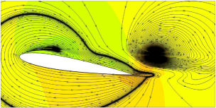
$\alpha=9.25^{\circ}$

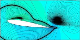
$\alpha=9.25^{\circ}$

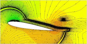
$\alpha=9.4^{\circ}$

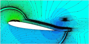
$\alpha=9.4^{\circ}$

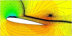
$\alpha=9.5^{\circ}$

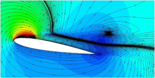
$\alpha=9.5^{\circ}$

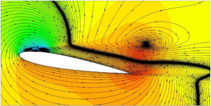
$\alpha=9.6^{\circ}$

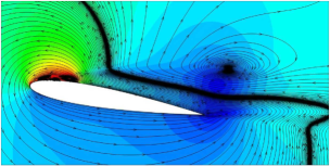
$\alpha=9.6^{\circ}$

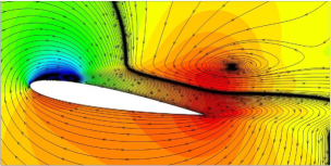
$\alpha=9.7^{\circ}$

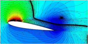
$\alpha=9.7^{\circ}$

Figure 2: Streamlines patterns of the time-averaged attached and separated phases of the oscillating-flow-field superimposed on colour maps of the time-averaged attached and separated phases of the oscillating-pressure-field for the angles of attack $\alpha=9.25^{\circ}$–$9.7^{\circ}$. Left: time-averaged attached-phase of the oscillating-flow-field estimated from the high-lift flow-field minus the mean-lift flow-field, $\Delta{\overline{U}}^{\mathrm{+}}$, $\Delta{\overline{V}}^{\mathrm{+}}$, and $\Delta{\overline{P}}^{\mathrm{+}}$. Right: time-averaged separated-phase of the oscillating-flow-field estimated from the low-lift flow-field minus the mean-lift flow-field, $\Delta{\overline{U}}^{\mathrm{-}}$, $\Delta{\overline{V}}^{\mathrm{-}}$, and $\Delta{\overline{P}}^{\mathrm{-}}$.

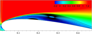
Time-averaged attached-phase of the flow-field.
      

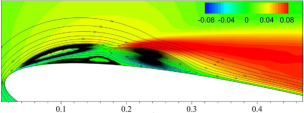
Time-averaged attached-phase of the oscillating-flow.

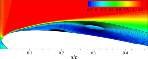
Time-averaged separated-phase of the flow-field.

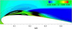
Time-averaged separated-phase of the oscillating-flow.

Figure 4: Streamlines patterns of the flow-field and the oscillating-flow-field superimposed on colour maps of the streamwise velocity component and the oscillating-streamwise-velocity, respectively, for the angle of attack of $9.6^{\circ}$. Left: time-averaged attached-phase (top) and separated-phase (bottom) flow-fields, $\widehat{U}$ & $\widehat{V}$ and $\widecheck{U}$ & $\widecheck{V}$, respectively. Right: time-averaged attached-phase (top) and separated-phase (bottom) of the oscillating-flow-field, $\Delta{\overline{U}}^{\mathrm{+}}$ & $\Delta{\overline{V}}^{\mathrm{+}}$ and $\Delta{\overline{U}}^{\mathrm{-}}$ & $\Delta{\overline{V}}^{\mathrm{-}}$, respectively.

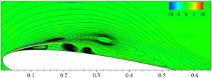
$\alpha=9.25^{\circ}$.

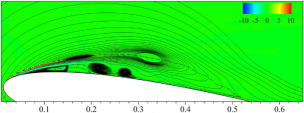
$\alpha=9.25^{\circ}$.

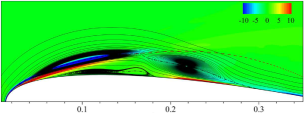
$\alpha=9.4^{\circ}$.

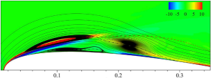
$\alpha=9.4^{\circ}$.

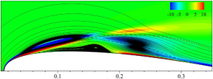
$\alpha=9.5^{\circ}$.

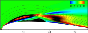
$\alpha=9.5^{\circ}$.

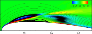
$\alpha=9.6^{\circ}$.

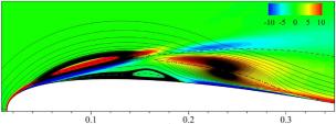
$\alpha=9.6^{\circ}$.

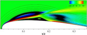
$\alpha=9.7^{\circ}$.

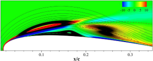
$\alpha=9.7^{\circ}$.

Figure 5: Streamlines patterns of the time-averaged attached and separated phases of the oscillating-flow-field superimposed on colour maps of the time-averaged attached and separated phases of the oscillating-spanwise-vorticity for the angles of attack $\alpha=9.25^{\circ}$–$9.7^{\circ}$. The red dashed line displays the streamline that bounds the LSB in the mean sense. The black dash-dot line denotes the contour line at which the time-average oscillating-streamwise-velocity equals zero. Left: time-average attached-phase of the oscillating-flow-field estimated from the high-lift flow minus the mean-lift flow-field, $\Delta{\overline{U}}^{\mathrm{+}}$ and $\Delta{\overline{V}}^{\mathrm{+}}$. Right: time-average separated-phase of the oscillating-flow estimated from the low-lift flow minus the mean-lift flow-field, $\Delta{\overline{U}}^{\mathrm{-}}$ and $\Delta{\overline{V}}^{\mathrm{-}}$.

The conditional time-averaging, described and used in Eljack et al. (2018b), defines the time-average of an instantaneous variable of the flow-field, $\psi$, on three different levels a high-lift average, a low-lift average, and a mean-lift average. The mean-lift average of the variable ($\overline{\psi}$) is simply the time-average of all data samples of the variable. The high-lift average of the variable ($\widehat{\psi}$) is the time-average of all data samples that have values higher than the mean values. The low-lift average of the variable ($\widecheck{\psi}$) is the average of all data samples that have values less than the mean values. When the lift coefficient signal is Gaussian, the high-lift and low-lift averages of the variable represent the attached and separated flow-field in the statistical sense, respectively. In this sense, one can define a time-averaged surplus ($\Delta{\overline{\psi}}^{\mathrm{+}}$) and deficit ($\Delta{\overline{\psi}}^{\mathrm{-}}$) of the flow variable above and below that of the mean-flow, respectively. Thus, the time-averaged surplus and deficit of the variable are given by subtracting the mean-lift average of the variable from the high-lift average of the variable and the low-lift average of the variable, respectively. Hence, the time-averaged surplus of the flow-field is estimated from the high-lift flow-field minus the mean-lift flow-field, $\Delta{\overline{\psi}}^{\mathrm{+}}=\widehat{\psi}-\overline{\psi}$. The time-averaged deficit of the flow-field is estimated from the low-lift flow-field minus the mean-lift flow-field, $\Delta{\overline{\psi}}^{\mathrm{-}}=\widecheck{\psi}-\overline{\psi}$. For a Gaussian lift coefficient signal, the time-averaged surplus and deficit of the variable above and below the mean feature the time-averaged attached-phase and separated-phase of the oscillating-flow-field, respectively.
Figures 2 and 3 show streamlines patterns of the time-averaged attached-phase of the oscillating-flow-field, $\Delta{\overline{U}}^{\mathrm{+}}$ and $\Delta{\overline{V}}^{\mathrm{+}}$, and the time-averaged separated-phase of the oscillating-flow-field, $\Delta{\overline{U}}^{\mathrm{-}}$ and $\Delta{\overline{V}}^{\mathrm{-}}$, superimposed on colour maps of the time-averaged attached-phase of the oscillating-pressure-field, $\Delta{\overline{P}}^{\mathrm{+}}$, and the time-averaged separated-phase of the oscillating-pressure-field, $\Delta{\overline{P}}^{\mathrm{-}}$, respectively, at the angles of attack $\alpha=9.25^{\circ}$–$10.5^{\circ}$. As seen in the figures, the time-averaged attached and separated phases of the oscillating-flow-field are rotating in a closed loop around the aerofoil in the clockwise and the anti-clockwise direction, respectively. A triad of three vortices, two co-rotating vortices (TCV) and a secondary vortex lies beneath them, and counter-rotating with them is formed in the vicinity of the leading-edge on the suction surface of the aerofoil in a region almost coincide with that of the LSB. A large vortex is located above the aerofoil trailing-edge and counter-rotates with the oscillating-flow-field adjacent to the aerofoil surface. This vortex acts as a wheel that pushes and guides the oscillating-flow-field towards the aerofoil surface and forces it to be directed tangentially to the aerofoil surface. The origin of this vortex is not known yet, i.e., is it created locally by the oscillating-flow-field or does it originate somewhere upstream the trailing-edge and advects downstream by the flow. Hereafter, this vortex will be referred to as the “guide-vortex”. The shape and strength of the guide-vortex vary with the angle of attack as seen in the figures. The time-averaged attached-phase of the flow-field sets the conditions for the LSB to be reformed after it bursts. Consequently, the pressure drops in the vicinity of the LSB and an adverse pressure gradient (APG) is formed along the aerofoil chord. When the LSB burst, the flow separates creating a high-pressure region in the vicinity of the leading-edge and a low-pressure region in the vicinity of the trailing-edge. Hence, a favourable pressure gradient (FPG) along the aerofoil chord is formed. When the direction of the time-averaged oscillating-flow-field is clock-wise, it adds momentum to the boundary layer, and the flow remains attached against the APG. When the oscillating-flow-field rotates in the anti-clockwise direction, it subtracts momentum from the boundary layer and drives the flow to separate despite the FPG. It seems that this triad of vortices, the gradient of the oscillating-pressure, and changes in the turbulent kinetic energy along the separated shear layer are interlinked, govern, and sustain the LFO. However, the details of the rotation of this triad and how it adjusts the frequency of the flow oscillation are lost in the averaging process. Most importantly, how this triad controls the bursting and stability of the LSB.
Figure 4 shows zoom-in plots of streamlines patterns of the flow-field and streamlines patterns of the oscillating-flow-field superimposed on colour maps of the streamwise velocity component of the flow-field and the oscillating-streamwise-velocity, respectively, for the angle of attack of $9.6^{\circ}$. The left-hand side of the figure shows the time-averaged attached (top) and the time-averaged separated (bottom) flow-fields, and the right-hand side of the figure displays the time-averaged attached (top) and the time-averaged separated (bottom) oscillating-flow-fields. As seen in the figure, the upstream vortex of the TCV (UV) is driven by the gradient of the oscillating-velocity across the laminar portion of the separated shear layer and is faithfully aligned with it. The UV front tip forms a half-saddle on the aerofoil surface just upstream the separation point of the shear layer, and its rear end forms a full-saddle. The downstream vortex of the TCV (DV) is submerged entirely inside the region of the LSB and aligned such that its front tip forms a full-saddle with the UV while its rear tip forms a half-saddle on the aerofoil surface upstream the reattachment point. The secondary vortex act as a roller support that facilitates the rotation and orientation of the TCV. The focus of the DV of the TCV is located just upstream and below that of the LSB, in the mean sense. However, the orientation of the triad of vortices, in the mean sense, changes with the angle of attack. Most importantly, instantaneous as well as spatial orientation of the triad of vortices seems to play a profound role on the stability of the LSB and the sustainability of the LFO.
Figures 5 and 6 show streamlines patterns of the time-averaged attached and separated phases of the oscillating-flow-field superimposed on colour maps of the time-averaged attached and separated flow phases of the oscillating-spanwise-vorticity for the angles of attack $\alpha=9.25^{\circ}$–$10.5^{\circ}$. The left-hand side of the figures shows the time-averaged attached-phase of the oscillating-flow-field estimated from the high-lift flow minus the mean-lift flow, $\Delta{\overline{U}}^{\mathrm{+}}$ and $\Delta{\overline{V}}^{\mathrm{+}}$. The right-hand side of the figures shows the time-averaged separated-phase of the oscillating-flow-field estimated from the low-lift flow minus the mean-lift flow, $\Delta{\overline{U}}^{\mathrm{-}}$ and $\Delta{\overline{V}}^{\mathrm{-}}$. The figures are zoomed in such a way that the orientation of the triad of vortices and how it varies with the angle of attack can be examined. The red dashed line displays the streamline that bounds the LSB in the mean sense. The black dash-dot line denotes the contour line at which the time-averaged oscillating-streamwise-velocity equals zero. It is evident that the oscillating-flow-field rotates in the clockwise direction during the attached-phase and rotates in the anti-clockwise direction during the separated-phase of the flow-field. It is noted that each vortex of the triad of vortices is aligned along a part of the dash-dot line.
The conditional time-averaging employed in the present study to obtain the attached and separated phases of the oscillating-flow-field takes into account contributions from all vortical structures, in the mean sense, regardless of their frequency and size. Thus, the time-averaged oscillating-flow-field captures the spatial evolution of all flow modes in a single snapshot. However, some oscillating-flow features could be obscured considering their relatively low amplitude. Therefore, the appearance of the time-averaged oscillating-flow-field reflects the shape of flow features that have the highest magnitude.
At the angle of attack of $9.0^{\circ}$, not shown here, the time-averaged attached and separated phases of the oscillating-flow-field form a single vortex above the streamline that bound the LSB. The vortex is stretched and break into two co-rotating vortices as the angle of attack is increased to $9.25^{\circ}$. These two co-rotating vortices are similar to the previously discussed TCV. However, it seems that these two co-rotating vortices gain momentum as the angle of attack increases. Thus, they become more pronounced in shape and magnitude as the angle of attack is increased. The TCV at the angle of attack of $9.25^{\circ}$ does not have enough energy to change the flow-field globally. The TCV could only extract energy from the oscillating-flow-field and redistribute this energy to remain in equilibrium. While doing this, the TCV elongate the time-scale of the oscillating-flow-field cycle and consequently reduce the frequency of the flow-oscillation below that of the bluff-body shedding frequency. Furthermore, the presence of the TCV in the flow-field changes the magnitude of the oscillating-flow-field, decreases the mean lift coefficient, increases the mean drag coefficient, and deteriorates the performance of the aerofoil.
At the angle of attack of $9.4^{\circ}$ a drastic change in the time-averaged attached and separated phases of the oscillating-flow-field takes place. The triad of vortices has enough energy to dominate the time-averaged oscillating-flow-field. The UV of the TCV elongates and moves upstream until its front tip forms a half-saddle that rests on the aerofoil surface just upstream the separation point of the shear layer. The UV is anchored to the laminar portion of the separated shear layer; thus, it preserves its shape and position, and remains erected above the separated zone. The secondary vortex, which lies beneath the TCV, is combined into one coherent vortex at this angle of attack. Whereas, at the angles of attack of $9.0^{\circ}$ and $9.25^{\circ}$ it was less coherent and splattered into two or three small vortices, in the mean sense. The most dramatic and important change that takes place in the orientation of the TCV is that of the DV. The downstream vortex is elongated just like the UV and oriented such that its rear tip forms a half-saddle on the aerofoil surface and entirely resides in the region of the LSB. However, the DV could preserve neither its shape nor its position. Its front tip forms a full-saddle with the UV, and its orientation with respect to the UV is dependent on the angle of attack, in the mean sense. What is important about this orientation is that the TCV are aligned in such a way that the UV could slide over the DV. While the UV is extracting energy from the mean flow, it gains more and more momentum until it is saturated. Then, the UV slides over the DV, expands, and advects downstream. When the UV expands, it changes the direction of rotation of the oscillating-flow-field. Hence, if the flow is attached, it will separate as a consequence of the expansion of the UV and vice versa. Thus, the conditions for the LSB bursting is that the UV of the TCV has enough energy and the TCV are oriented in such a way that the UV could slide above the DV. The ability of the UV to extract energy from the mean flow depends primarily on the gradient of the oscillating-velocity across the laminar portion of the separated shear layer. Therefore, the primary cause that triggers the instability of the LSB and initiates the LFO is the gradient of the oscillating-velocity across the laminar portion of the separated shear layer. This does not only reveal the bursting condition for the LSB, but it also reveals the mechanism that governs and sustains the LFO.
As the angle of attack is further increased to $9.5^{\circ}$, the UV expands intermittently. Hence, the LSB is intact with intermittent occasions on which it bursts. At this angle of attack, the mean flow is attached. Therefore, the occasional expansion of the UV and the subsequent bursting of the LSB separate the flow intermittently. The transition of the strength and orientation of the triad of vortices continues in the same manner until the LFO process becomes regular and more pronounced in the magnitude of oscillation at the angle of attack of $9.8^{\circ}$. As the angle of attack increases, the mean flow becomes separated, and the LSB does not form. The UV of the TCV extracts less energy from the mean flow as the gradient of the oscillating-velocity across the laminar portion of the separated shear layer decreases. However, the strength of the UV reaches the threshold required for it to expand and reattach the flow-field intermittently. As the flow reattaches, the conditions for the formation of the LSB are met, and the LSB forms in the vicinity of the leading-edge. Therefore, the flow-field at this angle of attack remains separated with frequent reattachments. As the angle increases, the UV expands less frequently, and the flow-field remains separated for longer time intervals. The aerofoil eventually undergoes a full stall when the angle of attack is further increased.

2.2 The origin of the oscillating-flow-field

The oscillating-flow and the velocity gradient across the laminar portion of the separated shear layer are observed in all of the investigated angles of attack including at zero angle of attack. However, the magnitude and frequency of the oscillation vary with the angle of attack. The origin of the oscillation is the instability at the trailing-edge that generates and sustains the von Karman alternating vortices. In harmony with the alternating vortices at the trailing-edge, the stagnation point at the vicinity of the leading-edge pitches up and down. The Strouhal number of the oscillating-flow at low to moderate angles of attack fluctuates around that of the bluff-body shedding of around $0.2$. However, the interaction between the tailing-edge instability, the triad of vortices, and the gradient of the oscillating-pressure shifts the frequency of the resultant oscillating-flow to lower values. The more energy the UV of the TCV extracts from the mean-flow, the more it will be able to elongate the time-scale of the cycle of the oscillating-flow and consequently lowers its frequency. The ability of the UV to extract energy from the mean-flow depends primarily on the gradient of the oscillating-velocity across the laminar portion of the separated shear layer. As the gradient of the oscillating-velocity is proportional to the angle of attack, the UV gains more momentum as the angle of attack increases and can further lower the frequency of the LFO and increases its magnitude of oscillation.

2.3 Conditional phase-average of the oscillating-flow-field

The conditional time-average of the oscillating-flow-field not only characterised the behaviour of the flow in the mean sense, but it also revealed a profound triad of vortices that sets the bursting conditions of the LSB and sustains the LFO. However, temporal and spatial information are lost in the averaging process. Therefore, the conditional-averaging implemented in $\S$ 2.1 was extended to cover a broader range of levels; hence, help to keep some phase information. The previously defined conditional time-average on three levels (high-lift, low-lift, and man lift) was expanded to a series of $37$ intervals that give continues phase information of one complete cycle. Figure 1 illustrates the conditional phase-averaging process. The right-hand side of the figure shows time history of the lift coefficient at the angle of attack of $9.80^{\circ}$. The black line denotes the lift coefficient signal, and the red line displays the low-pass filtered lift coefficient. The left-hand side of the figure shows one sinusoidal cycle with a magnitude range of that of the low-pass filtered lift coefficient divided into $36$ equally distributed phases. The phase-averaging process is implemented in the same manner described and used in Eljack et al. (2018b) for the conditional time-averaging. Low-pass filtering the data before conditionally phase-averaging it improves the phase-averaging process significantly. The primary objective is to examine the evolution of the low-frequency flow modes; thus, filtering out the high frequencies does not affect the resulting phase-averaged flow-field. The low-pass filtered lift coefficient signal was split into an ascending part in which the lift is increasing with time and a descending part. The phase-averaging process was applied to the ascending low-pass filtered lift coefficient and its corresponding low-pass filtered data points for the phases intervals from $\Phi=0^{\circ}$ to $\Phi=180^{\circ}$. The descending low-pass filtered lift coefficient and its corresponding low-pass filtered data points are used in the phase-averaging process in the phases intervals from $180^{\circ}<\Phi<360^{\circ}$. The flow-field studied in the present work involves exceptionally low frequency and one cycle span over $25$ non-dimensional time units. Collecting data that covers one hundred cycles is not feasible in numerical simulation. However, the conditional phase-averaging described above enhances the statistics and give much better estimate. Hereafter, the conditionally phase-average and phase-average terms will be used interchangeably. For a flow variable $\psi$ the decomposition is as follows:

$$\psi=\overline{\psi}+\underbrace{\widetilde{\psi}+{\psi}^{\prime}\mkern-1.2mu}_{{\psi}^{\prime\prime}\mkern-1.2mu}$$ (1)

Where, $\overline{\psi}$ is the mean of the variable, $\widetilde{\psi}$ is the conditionally phase-averaged, and ${\psi}^{\prime}\mkern-1.2mu$ is the fluctuations of the variable “turbulent-fluctuations”.

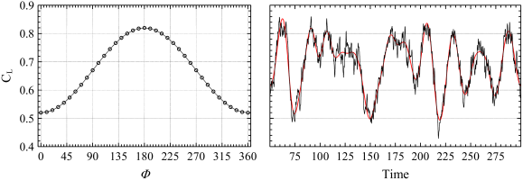
Figure 1: The conditional phase-averaging process. Left: One sinusoidal cycle with a magnitude range of that of the low-pass filtered lift coefficient divided into $36$ equally distributed phases. Right: The black line displays the time history of the lift coefficient, and the red line denotes the low-pass filtered lift coefficient at the angle of attack of $9.80^{\circ}$.

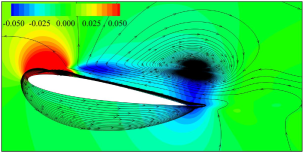
$\Phi=0^{\circ}$

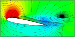
$\Phi=40^{\circ}$

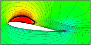
$\Phi=90^{\circ}$

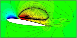
$\Phi=130^{\circ}$

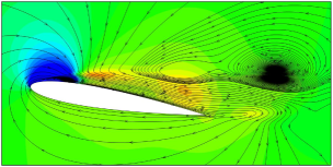
$\Phi=180^{\circ}$

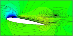
$\Phi=220^{\circ}$

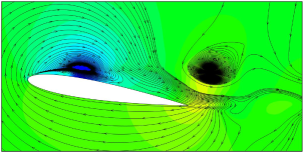
$\Phi=270^{\circ}$

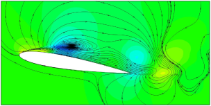
$\Phi=310^{\circ}$

Figure 7: Streamlines patterns of the phase-averaged oscillating-flow-field superimposed on colour maps of the phase-averaged oscillating-pressure for the angle of attack of $9.4^{\circ}$.

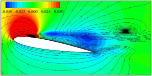
$\Phi=0^{\circ}$

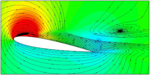
$\Phi=40^{\circ}$

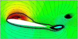
$\Phi=90^{\circ}$

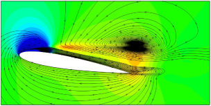
$\Phi=130^{\circ}$

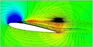
$\Phi=180^{\circ}$

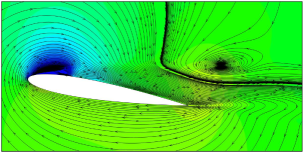
$\Phi=220^{\circ}$

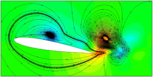
$\Phi=270^{\circ}$

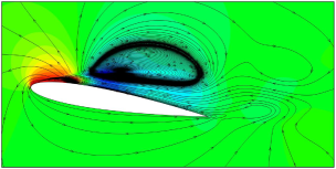
$\Phi=310^{\circ}$

Figure 8: Streamlines patterns of the phase-averaged oscillating-flow-field superimposed on colour maps of the phase-averaged oscillating-pressure for the angle of attack of $9.5^{\circ}$.

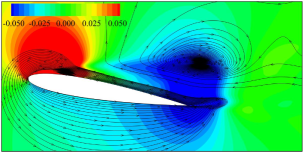
$\Phi=0^{\circ}$

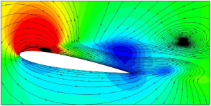
$\Phi=40^{\circ}$

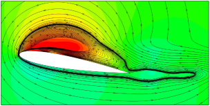
$\Phi=90^{\circ}$

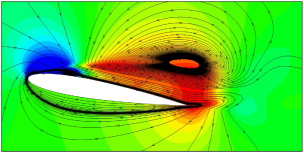
$\Phi=130^{\circ}$

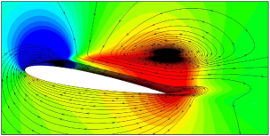
$\Phi=180^{\circ}$

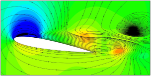
$\Phi=220^{\circ}$

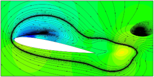
$\Phi=270^{\circ}$

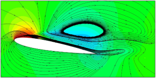
$\Phi=310^{\circ}$

Figure 9: Streamlines patterns of the phase-averaged oscillating-flow-field superimposed on colour maps of the phase-averaged oscillating-pressure for the angle of attack of $9.7^{\circ}$.

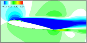
$\Phi=0^{\circ}$

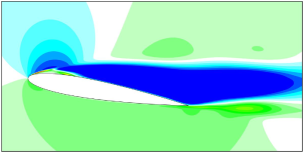
$\Phi=40^{\circ}$

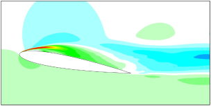
$\Phi=90^{\circ}$

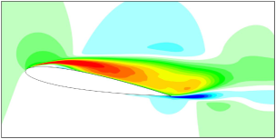
$\Phi=130^{\circ}$

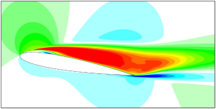
$\Phi=180^{\circ}$

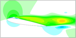
$\Phi=220^{\circ}$

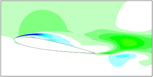
$\Phi=270^{\circ}$

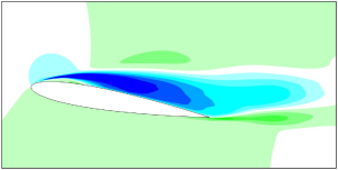
$\Phi=310^{\circ}$

Figure 10: Colour maps of the phase-averaged oscillating-streamwise-velocity for the angle of attack of $9.7^{\circ}$.

Figure 1 shows that the flow is fully separated at the phase angle $\Phi=0^{\circ}$ and the lift coefficient is at its minimum value. Figure 7 shows streamline patterns of the phase-averaged oscillating-flow-field superimposed on colour maps of the phase-averaged oscillating-pressure for the angle of attack of $9.4^{\circ}$. As shown in the figure, at the phase angle $\Phi=0^{\circ}$ the oscillating-flow is rotating in the anti-clockwise direction. Thus, the oscillating-flow adjacent to the aerofoil surface on the suction surface subtracts momentum from the boundary layer and separates the flow. The colour maps of the oscillating-pressure indicate that the flow is separated and an FPG is building up along the aerofoil chord. The oscillating-flow rotates in the anti-clockwise direction and reduces the gradient of the streamwise velocity component across the shear layer. Thus, the transition location is expected to be at its furthest downstream position. The TCV rotate in the anti-clockwise direction, the UV of the TCV is storing energy, and the secondary vortex rotates in the clock-wise direction.
At the phase angle of $\Phi=40^{\circ}$ the UV of the TCV a little bit pop-up above the DV. The magnitude of the oscillating-pressure decreases, and the FPG along the aerofoil chord weakens. The oscillating-flow-field losses momentum, and the gradient of the streamwise velocity across the shear layer increases. Hence, the transition point is expected to move a little bit upstream. At the phase angle of $\Phi=90^{\circ}$ the UV is saturated with energy, expands, and advects downstream. The UV of the TCV is rotating in the anti-clockwise direction. Thus, as the UV expands, the direction of the oscillating-flow flips globally and the oscillating-flow rotates in the clockwise direction. Consequently, the oscillating flow adds momentum to the boundary layer and the flow-field attaches as seen at $\Phi=130^{\circ}$. An APG starts to build up along the aerofoil chord. There are $40$ or $50$ degrees between each of the snapshots, and the most important ones are these between $40$ and $130$ because they contain the information on how the UV expands and advects.
As the oscillating-flow rotates in the clockwise direction so are the TCV. The UV after it expands, advects downstream, and goes through a series of modifications, it eventually forms the guide-vortex mentioned earlier and its origin was not clear. The flow-field is attached during the phases $\Phi=180^{\circ}$ and $\Phi=220^{\circ}$. At the phase angle of $\Phi=180^{\circ}$ the flow is fully attached, the APG at its maximum magnitude and the lift coefficient is at its maximum value as seen in figure 1. After that, the UV raises a little bit above the DV, again, at the phase angle $\Phi=220^{\circ}$. The UV, rotating in the clockwise direction now, continues to rise above the DV and gain more momentum until it saturates with energy, expands and the flow separates again. The guide-vortex continues to deform, and the flow continues to separate until the lift coefficient returns to its minimum at the phase angle of $360^{\circ}$. Meanwhile, the point of maximum turbulent kinetic energy, transition location, moves upstream and downstream in accordance with the direction of rotation of the oscillating-flow.
It is noted that at the angle of attack of $9.4^{\circ}$ the gradient of the oscillating-velocity across the laminar portion of the separated shear layer occasionally reaches the threshold required for the UV of the TCV to expand. Accordingly, the UV expands and the LSB bursts intermittently. As the mean-flow is attached at this angle of attack, the flow remains attached and separates intermittently. Therefore, the lift coefficient is at its maximum value with intermittent occasions at which the lift drops below its maximum value. However, the gradient of the oscillating-velocity is relatively small, and the UV extracts relatively small fraction of energy from the mean flow. Thus, the amplitude of the intermittent oscillations in the flow-field and the lift coefficient is relatively small. The gradient of the oscillating-velocity and the capacity of the UV to store energy before expanding are proportional to the angle of attack. Consequently, the UV causes more pronounced oscillations in the oscillating-flow-field and the aerodynamic coefficients as the angle of attack increases. Furthermore, the time required for the oscillating-flow-field to change its direction of rotation is proportional to the initial energy input by the UV of the TCV. Hence, the UV capability in reducing the frequency of the LFO and increasing the amplitude of oscillation increases as the angle of attack is increased. As shown in figures 5 and 6 the magnitude of the oscillating-spanwise-vorticity increases as the angle of attack is increased. This is indicative that the gradient of the oscillating-velocity across the laminar portion of the separated shear layer increases as the angle of attack is increased. Thus, the strength of the UV is proportional to the angle of attack. Consequently, the magnitude of the oscillating-flow increases as shown in figure 8. The expansion, advection, and reformation of the UV become more regular and pronounce in magnitude in the angle of attack of $9.5^{\circ}$ as seen in the figure.
Figure 9 shows streamline patterns of the phase-averaged oscillating-flow-field superimposed on colour maps of the phase-averaged oscillating-pressure for the angle of attack of $9.7^{\circ}$. Figure 10 shows colour maps of the phase-averaged oscillating-streamwise-velocity for the angle of attack of $9.7^{\circ}$. At the phase angle $\Phi=0^{\circ}$, the flow is separated, the oscillating-streamwise-velocity is negative on the suction surface of the aerofoil, and the FPG along the aerofoil chord is at its maximum magnitude in the cycle. The magnitude of the oscillating-streamwise-velocity increases and the amplitude of the FPG decreases at the phase angle of $\Phi=40^{\circ}$. The magnitude of the oscillating-streamwise-velocity and the amplitude of the FPG fluctuate around zero at the phase angle of $90^{\circ}$. As the oscillating-flow decays, the flow reaches an equilibrium state, and the oscillation in the flow vanishes. However, the UV of the TCV is saturated with energy. Thus, the UV expands, the flow-field attaches, and a new imbalance is created at the phase angle of $90^{\circ}$. As the flow attaches, the oscillating-streamwise-velocity becomes positive, and an APG builds up along the aerofoil chord as seen in the phase angles of $130^{\circ}$, $180^{\circ}$, and $220^{\circ}$. The flow is fully attached at $\Phi=180^{\circ}$, the oscillating-streamwise-velocity at its maximum magnitude above the mean streamwise velocity, and the APG is at its maximum amplitude. After that, the oscillating-streamwise-velocity and the APG decrease until they become zero at $\Phi=270^{\circ}$. The oscillating-flow-field has no enough momentum to keep the boundary layer attached. Consequently, the flow reaches a new equilibrium, and the UV of the TCV expands and repels the attached-flow and forces it to separate abruptly at $\Phi=310^{\circ}$. As the process reverses its direction, the oscillating-streamwise-velocity becomes negative again, and an FPG builds up along the aerofoil chord as seen in $\Phi=310^{\circ}$ and $0^{\circ}$. The transition process starts at the angle of attack of $9.25^{\circ}$ and continues until the LFO becomes self-sustained at the angle of attack of $9.7^{\circ}$

2.4 The underlying mechanism

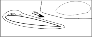
$\Phi=0^{\circ}$

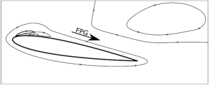
$\Phi=45^{\circ}$

$\Phi=90^{\circ}$

$\Phi=135^{\circ}$

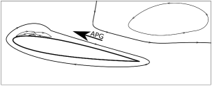
$\Phi=180^{\circ}$

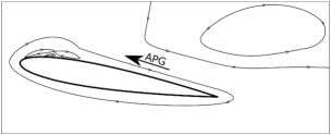
$\Phi=225^{\circ}$

$\Phi=270^{\circ}$

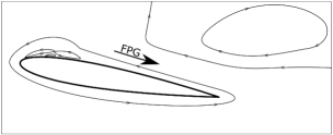
$\Phi=315^{\circ}$

Figure 11: A model that describe the underlying mechanism behind the self-sustained quasi-periodic low-frequency flow oscillation featuring the bursting and reformation cycle of a laminar separation bubble. Line and arrow width displays the strength of the pressure gradient along the aerofoil chord, the oscillating-flow, and the UV of the TCV.

The conditional phase-averaging of the data revealed the details of how the triad of vortices controls the time-scale of the LFO. However, the process is not perfectly periodic especially at this low Reynolds number. Therefore, the above discussion on the underlying mechanism is summarised in figure 11. The LFO cycle is assumed to be sinusoidal and divided into eight equally distributed phases. The sequence of phase angles and events matches that of the above data analysis. The self-sustained separation and reattachment of the flow repeat periodically in the following sequence of events:
$\bm{\Phi}\bm{=}\bm{0}^{\bm{\circ}}$: The flow is fully separated. The LSB is not present. The oscillating-streamwise-velocity is negative and at its minimum amplitude. The oscillating-flow and the TCV rotate in the anti-clockwise direction. The gradient of the oscillating-velocity across the laminar portion of the separated shear layer at its maximum magnitude, and the energy extraction by the UV of the TCV at its maximum rate. The velocity gradient across the separated shear layer at its minimum magnitude. Thus, the transition process via the Kelvin–Helmholtz instability is delayed, and the transition location is at its furthest downstream position, “late-transition”. The pressure gradient along the aerofoil chord is favourable and at its maximum magnitude. The fluctuating lift coefficient is negative and at its minimum magnitude.
$\bm{\Phi}\bm{=}\bm{45}^{\bm{\circ}}$: The oscillating-streamwise-velocity, the velocity gradient across the separated shear layer, and the fluctuating lift coefficient increase. Thus, the transition location moves a little pit upstream. The gradient of the oscillating-velocity across the laminar portion of the separated shear layer, the rate of energy extraction by the UV of the TCV, and the gradient of the pressure along the aerofoil chord decrease.
$\bm{\Phi}\bm{=}\bm{90}^{\bm{\circ}}$: The amplitude of the oscillating-streamwise-velocity, the velocity gradient across the separated shear layer, the gradient of the oscillating-velocity across the laminar portion of the separated shear layer, the rate of energy extraction by the UV of the TCV, the gradient of the pressure along the aerofoil chord, and the fluctuating lift coefficient become almost zero. Hence, the transition location is determined naturally by the Kelvin–Helmholtz instability. Therefore, the flow-field reaches an equilibrium state. The UV of the TCV saturates with energy, expands, advects downstream, and starts a new imbalance. The direction of the oscillating-flow flips globally and the TCV rotate in the clockwise direction. The oscillating-flow adds momentum to the separated boundary layer, and the flow attaches.
$\bm{\Phi}\bm{=}\bm{135}^{\bm{\circ}}$: The flow is attached. The LSB is present and intact. The oscillating-streamwise-velocity becomes positive. The oscillating-flow rotates in the clockwise direction. The velocity gradient across the separated shear layer increases. Thus, the transition process via the Kelvin–Helmholtz instability is accelerated, and the transition location moves a little pit upstream. An adverse pressure gradient forms along the aerofoil chord. The fluctuating lift coefficient is positive.
$\bm{\Phi}\bm{=}\bm{180}^{\bm{\circ}}$: The flow is fully attached. The oscillating-streamwise-velocity is positive and at its maximum amplitude. The oscillating-flow and the TCV rotate in the clockwise direction. The gradient of the oscillating-velocity across the laminar portion of the separated shear layer at its maximum magnitude, and the energy extraction by the UV of the TCV at its maximum rate. The velocity gradient across the separated shear layer at its maximum value. Consequently, the transition process via the Kelvin–Helmholtz instability is further accelerated, and the transition location is at its furthest upstream position, “early-transition”. The adverse pressure gradient along the aerofoil chord at its maximum magnitude. The fluctuating lift coefficient is positive and at its maximum amplitude.
$\bm{\Phi}\bm{=}\bm{225}^{\bm{\circ}}$: The oscillating-streamwise-velocity, the velocity gradient across the separated shear layer, the gradient of the oscillating-velocity across the laminar portion of the separated shear layer, the rate of energy extraction by the UV of the TCV, the gradient of the pressure along the aerofoil chord, and the fluctuating lift coefficient decrease. The transition location moves a little pit downstream.
$\bm{\Phi}\bm{=}\bm{270}^{\bm{\circ}}$: The flow-field reaches a new equilibrium state. The UV of the TCV saturates with energy, expands, advects downstream, and starts a new disequilibrium. The direction of the oscillating-flow flips globally and the TCV rotate in the anti-clockwise direction. The oscillating-flow subtracts momentum from the boundary layer, and the flow separates again.
$\bm{\Phi}\bm{=}\bm{315}^{\bm{\circ}}$: The oscillating-streamwise-velocity becomes negative again. The oscillating-flow rotates in the anti-clockwise direction. The velocity gradient across the separated shear layer decreases. Thus, the transition process via the Kelvin–Helmholtz instability is further delayed, and the transition location moves a little pit downstream. A favourable pressure gradient forms along the aerofoil chord. The fluctuating lift coefficient is negative and decreasing.
Thus, the stability of the LSB and the sustainability of the LFO phenomenon, in a naturally evolving flow, are controlled by the following parameters:

1. The strength and the direction of rotation of the oscillating-flow.

2. The velocity gradient across the separated shear layer.

3. The transition location along the separated shear layer.

4. The gradient of the oscillating-velocity across the laminar portion of the separated shear layer.

5. The strength and dynamics of the triad of vortices.

6. The ability of the UV of the TCV to extract energy from the mean-flow.

7. The gradient of the oscillating-pressure along the aerofoil chord.

These parameters, hereafter the LFO-control-parameters, are interlinked. The process is self-sustained and quasi-periodic in a manner that once the oscillating-flow reaches an equilibrium, the UV expands and creates a new disequilibrium. However, sometimes the TCV reverse the process before the cycle is completed and the periodic cycle is disturbed. The present model confirms the observations of Tanaka (2004) about the guide-vortex that play an important role in the phenomenon. Most importantly, the model presented in the current work shows that the elegant modelling of the phenomenon carried out by Sandham (2008) is accurate in many aspects despite the fact that the underlying mechanism was not revealed at the time.

2.5 The disturbed cycles and the route to a full stall

Most of the previous experimental and numerical work that captured the LFO reported that some disturbed cycles do not resemble other regular cycles, Tanaka (2004) and Eljack (2017). The underlying mechanism presented in $\S$ 2.4 is assumed to be perfectly periodic. If the LFO-control-parameters are perfectly synchronised in such a way that they oscillate in-phase, then they will oscillate in harmony and drive the flow into equilibrium periodically. Thus, the LFO process would repeat periodically. Whereas, when the LFO-control-parameters are not synchronised, for reasons that are not clear now, irregular disturbed cycles that do not resemble other regular cycles are occasionally produced. The reason behind such disturbed cycles is that the sequence of events as described in $\S$ 2.4 is interrupted, and the process is reversed before it is completed. For instance, in figure 11, at $\Phi=45^{\circ}$ the flow-field is attaching and the lift coefficient is increasing. If the LFO-control-parameters are synchronised, the sequence of events will continue as usual to that at $\Phi=90^{\circ}$ and $135^{\circ}$. However, sometimes the process from $\Phi=45^{\circ}$ goes back to $\Phi=0^{\circ}$ instead of continuing to $\Phi=90^{\circ}$ and the periodic cycle is interrupted.
Another issue of major importance is the variation of the LFO cycle with the angle of attack and the route through which an aerofoil undergoes a full stall. As mentioned before, the oscillating-flow is present in all of the investigated angles of attack, including at zero angle of attack. The magnitude of the oscillation increases and the frequency of the oscillation decreases as the angle of attack is increased. As shown by Eljack et al. (2018b), the mean flow-field is attached at the angle of attack of $9.25^{\circ}$ and fully separated at the angle of attack of $10.5^{\circ}$. At the angle of attack of $9.25^{\circ}$, the mean-flow is attached, the UV of the TCV occasionally expands; consequently, the LSB bursts and the flow-field separates intermittently. As the angle of attack increases, the UV expands more frequently. At the angle of attack of $9.8^{\circ}$, the LFO becomes fully developed and quasi-periodic. At higher angles of attack, the mean-flow is separated. Sometimes the UV expands, the flow attaches, and the conditions for the reformation of the LSB are met. Consequently, the flow-field remains separated with intermittent attachments. As the angle of attack is further increased, the UV expands less frequently, and the flow-field remains separated for longer time intervals. At a critical angle of attack, the UV never expands, the flow-field remains separated, and the aerofoil undergoes a full stall.

2.6 Statistics of the conditionally phase-averaged oscillating-flow-field

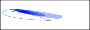
$\alpha=9.40^{\circ}$

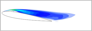
$\alpha=9.50^{\circ}$

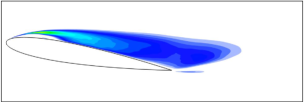
$\alpha=9.60^{\circ}$

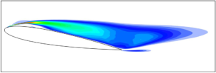
$\alpha=9.70^{\circ}$

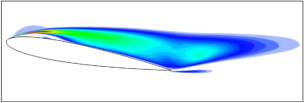
$\alpha=9.80^{\circ}$

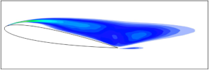
$\alpha=9.90^{\circ}$

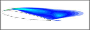
$\alpha=10.0^{\circ}$

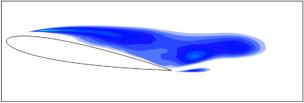
$\alpha=10.1^{\circ}$

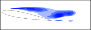
$\alpha=10.5^{\circ}$

Figure 12: Colour maps of the variance of the phase-averaged streamwise velocity component, $\overline{\widetilde{u}^{2}}$, for the angles of attack $\alpha=9.25^{\circ}$–$10.5^{\circ}$.

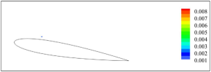
$\alpha=9.25^{\circ}$

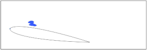
$\alpha=9.40^{\circ}$

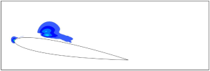
$\alpha=9.50^{\circ}$

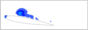
$\alpha=9.60^{\circ}$

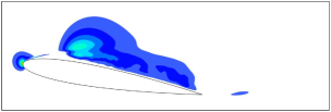
$\alpha=9.70^{\circ}$

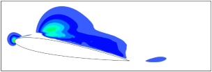
$\alpha=9.80^{\circ}$

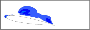
$\alpha=9.90^{\circ}$

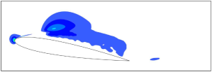
$\alpha=10.0^{\circ}$

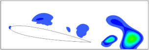
$\alpha=10.1^{\circ}$

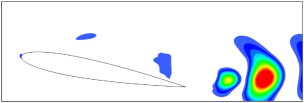
$\alpha=10.5^{\circ}$

Figure 13: Colour maps of the variance of the phase-averaged wall-normal velocity component, $\overline{\widetilde{v}^{2}}$, for the angles of attack $\alpha=9.25^{\circ}$–$10.5^{\circ}$.

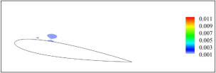
$\alpha=9.25^{\circ}$

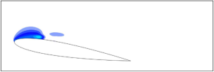
$\alpha=9.40^{\circ}$

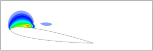
$\alpha=9.50^{\circ}$

$\alpha=9.60^{\circ}$

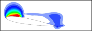
$\alpha=9.70^{\circ}$

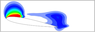
$\alpha=9.80^{\circ}$

$\alpha=9.90^{\circ}$

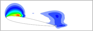
$\alpha=10.0^{\circ}$

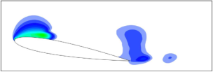
$\alpha=10.1^{\circ}$

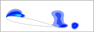
$\alpha=10.5^{\circ}$

Figure 14: Colour maps of the variance of the phase-averaged pressure, $\overline{\widetilde{p}^{2}}$, for the angles of attack $\alpha=9.25^{\circ}$–$10.5^{\circ}$.

A question was raised at this point of the analysis about the nature of the oscillating-flow over the LFO cycle. Does the oscillating-flow flap up and down, does it pulsate in the streamwise direction or both? To shed some light on the behaviour of the oscillating-flow, the conditionally phase-averaged oscillating-flow was used to estimate the variance of the phase-averaged oscillating-streamwise-velocity, $\overline{\widetilde{u}^{2}}$, oscillating-wall-normal-velocity, $\overline{\widetilde{v}^{2}}$, and the oscillating-pressure, $\overline{\widetilde{p}^{2}}$.
Figure 12 shows colour maps of the variance of the phase-averaged oscillating-streamwise-velocity, $\overline{\widetilde{u}^{2}}$, for the angles of attack $\alpha=9.25^{\circ}$–$10.5^{\circ}$. At the angle of attack of $9.25^{\circ}$, the figure displays no significant value of $\overline{\widetilde{u}^{2}}$ other than that along the shear layer. Thus, the flow is oscillating at this angle of attack with the minimum magnitude and mostly along the shear layer in the vicinity of the leading-edge. The flow oscillation extends along and around the shear layer at the angle of attack of $9.4^{\circ}$. The flow oscillation covers a wider region on the suction surface of the aerofoil, and has a more significant magnitude at higher angles of attack. The amplitude of oscillation continues to increase until it reaches a maximal value at the angle of attack of $9.8^{\circ}$. The magnitude of oscillation decreases as the angle of attack is further increased until it reaches an insignificant amplitude at the angle of attack of $10.5^{\circ}$.
Colour maps of the variance of the phase-averaged oscillating-wall-normal-velocity, $\overline{\widetilde{v}^{2}}$, for the angles of attack $\alpha=9.25^{\circ}$–$10.5^{\circ}$ are shown in figure 13. As seen in the figure, the wall-normal oscillations are mostly concentrated at the leading-edge and on the suction surface of the aerofoil. The significant oscillations of the wall-normal velocity component at the leading-edge are primarily due to the global oscillations in the flow-field. However, the maximum amplitude of oscillation at the angle of attack of $9.8^{\circ}$ is much smaller than that of the oscillating-streamwise-velocity component. Thus, the phase-averaged oscillating-flow is mostly pulsating in the streamwise direction rather than being flapping up and down on the suction surface of the aerofoil. At the angles of attack of $10.1^{\circ}$ and $10.5^{\circ}$ the oscillations in the wall-normal velocity shifts to a wake like oscillating mode. Furthermore, the magnitude of $\overline{\widetilde{v}^{2}}$ is considerably reduced at the leading-edge. Thus, at these angles of attack the oscillations of the wall-normal velocity does not convert effectively into a global oscillations in the flow-field but rather converts into a stronger flapping of the wake in the vicinity of the trailing-edge. Despite the relatively small magnitude of oscillation of the wall-normal velocity, it plays a profound role in initiating the global flow oscillation. Thus, it connects the tailing-edge and the leading-edge instabilities, and feeds the UV of the TCV.
Figure 14 shows colour maps of the variance of the phase-averaged oscillating-pressure. The $\overline{\widetilde{p}^{2}}$ is distributed in accordance with the gradient of the oscillating-pressure along the aerofoil chord as seen in the figure. The $\overline{\widetilde{p}^{2}}$ distribution highlights two important regions for the LFO and the stability of the LSB. The leading-edge where the LSB is formed and the triad of vortices are in action, and at the trailing-edge where the oscillating-pressure fluctuates significantly.

2.7 Statistics of the “turbulent-fluctuating” field

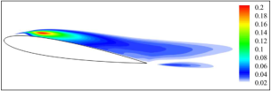
$\alpha=9.25^{\circ}$

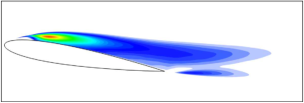
$\alpha=9.40^{\circ}$

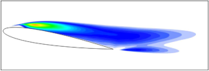
$\alpha=9.50^{\circ}$

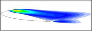
$\alpha=9.60^{\circ}$

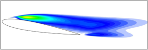
$\alpha=9.70^{\circ}$

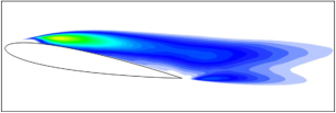
$\alpha=9.80^{\circ}$

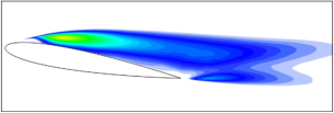
$\alpha=9.90^{\circ}$

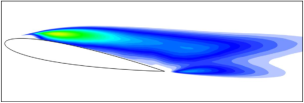
$\alpha=10.0^{\circ}$

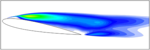
$\alpha=10.1^{\circ}$

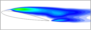
$\alpha=10.5^{\circ}$

Figure 15: Colour maps of the variance of the “turbulent fluctuations” of the streamwise velocity component, $\overline{{u^{\prime}\mkern-1.2mu}^{2}}$, for the angles of attack $\alpha=9.25^{\circ}$–$10.5^{\circ}$.

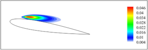
$\alpha=9.25^{\circ}$

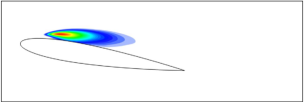
$\alpha=9.40^{\circ}$

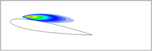
$\alpha=9.50^{\circ}$

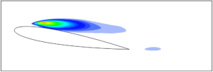
$\alpha=9.60^{\circ}$

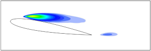
$\alpha=9.70^{\circ}$

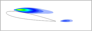
$\alpha=9.80^{\circ}$

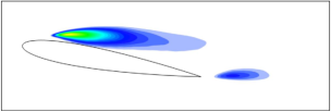
$\alpha=9.90^{\circ}$

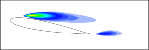
$\alpha=10.0^{\circ}$

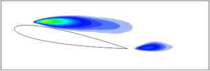
$\alpha=10.1^{\circ}$

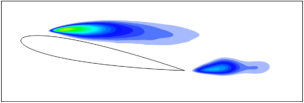
$\alpha=10.5^{\circ}$

Figure 16: Colour maps of the variance of the “turbulent fluctuations” of the pressure, $\overline{{p^{\prime}\mkern-1.2mu}^{2}}$, for the angles of attack $\alpha=9.25^{\circ}$–$10.5^{\circ}$.

The phase-averaged oscillations are characterised by large deterministic vortices that affects the flow-field globally. However, another type of oscillations is present in the flow-field. These are small random perturbations that grow in size and magnitude, breakup and merge, and very much characterise the turbulent flows. The former is referred to as phase-averaged oscillations or the periodic component, and the latter is referred to as the “turbulent fluctuations” or the random component. The term is always mentioned in the text inside quotation mark to highlight the fact that the flow could be laminar, transitional, or turbulent; therefore, referring to the fluctuations as turbulent does not imply that the flow underwent transition to turbulence.
Equation 1 shows how a flow variable $\psi$ is decomposed into mean, phase-averaged, and “turbulent fluctuations”. The equation is used to estimate the variance of the “turbulent fluctuations” of the streamwise velocity component, $\overline{{u^{\prime}\mkern-1.2mu}^{2}}$, and the variance of the “turbulent fluctuations” of the pressure, $\overline{{p^{\prime}\mkern-1.2mu}^{2}}$. Figure 15 displays colour maps of the $\overline{{u^{\prime}\mkern-1.2mu}^{2}}$ for the angles of attack $\alpha=9.25^{\circ}$–$10.5^{\circ}$. The streamwise fluctuations have significant magnitude along the separated shear layer and at the trailing-edge. It starts with a small amplitude at the laminar portion of the separated shear layer and increases along the shear layer. Hence, featuring the extraction of turbulent kinetic energy from the mean flow via the Kelvin–Helmholtz instability. At the angle of attack of $9.25^{\circ}$, the transition process takes place naturally by the Kelvin–Helmholtz instability, and the globally oscillating-flow does not affect the velocity gradient across the shear layer. Thus, the extraction of the turbulent kinetic energy from the mean and feeding it into the small-scales perturbations starts at the furthest upstream location along the shear layer, in the mean sense. As the angle of attack is increased, the velocity gradient across the separated shear layer is overwhelmed by the globally oscillating-flow. Consequently, the transition location oscillates significantly along the shear layer. Thus, the location of the maximum turbulent kinetic energy moves downstream, in the mean sense, as the angle of attack increases. At the angle of attack of $9.8^{\circ}$, the angle of maximum phase-averaged oscillations, $\overline{{u^{\prime}\mkern-1.2mu}^{2}}$ has a maximum value further downstream the leading-edge. The phase-averaged oscillations becomes insignificant as the angle of attack is further increased. Consequently, the location where $\overline{{u^{\prime}\mkern-1.2mu}^{2}}$ has a maximum moves upstream as the angle of attack is increased above the angle of $9.8^{\circ}$. The maximum value of $\overline{{u^{\prime}\mkern-1.2mu}^{2}}$ decreases as the angle of attack is increased as seen in the figure. At the angle of attack of $9.8^{\circ}$, the fluctuating flow is overwhelmed by the LFO, and the “turbulent fluctuations” reduces significantly downstream the separated shear layer.
There is no significant difference between the variance of the “turbulent fluctuations” of the wall-normal velocity component, $\overline{{v^{\prime}\mkern-1.2mu}^{2}}$, and the variance of the wall-normal velocity component, $\overline{{v^{\prime\prime}\mkern-1.2mu}^{2}}$. Obviously, this is because the phase-averaged component is much smaller compared to that of the “turbulent fluctuations”. Figure 16 displays $\overline{{p^{\prime}\mkern-1.2mu}^{2}}$ for the angles of attack $\alpha=9.25^{\circ}$ to $10.5^{\circ}$. As seen in the figure, $\overline{{p^{\prime}\mkern-1.2mu}^{2}}$ has no significant value at the leading-edge and along the laminar portion of the separated shear layer. Again, this is the location where the inviscid absolute instability is at action and most of the pressure fluctuations are phase-averaged not “turbulent”. Also, in the vicinity of the trailing-edge, the fluctuations in the pressure are due to large vortices and mostly phase-averaged.
In summary, small-scale vortical structures that contribute to the “turbulent fluctuations” are primarily extracted and maintained by the Kelvin–Helmholtz instability along the shear layer. Thus, the variance of the “turbulent fluctuations” has significant magnitude along the separated shear layer in the vicinity of the leading-edge. Also, the instability at the trailing-edge contributes significantly to the small-scale perturbations. Thus, the variance of the “turbulent fluctuations” increases in the vicinity of the trailing-edge. On the contrary, large-scale vortices contribute to the variance of the phase-averaged oscillations. These vortices are generated and sustained by the inviscid instability across the laminar portion of the separated shear layer. Thus, the phase-averaged oscillations have significant amplitude on both sides of the laminar portion of the separated shear layer. Furthermore, these large vortices advect downstream and contribute significantly to the flow variations at the trailing-edge. Thus, the phase-averaged oscillations have a considerable magnitude in the vicinity of the trailing-edge. Finally, the aforementioned discussion confirms the observations reported by Eljack et al. (2018b) that the perturbations in the streamwise velocity and the pressure are extracted by the global flow oscillation in addition to the Kelvin–Helmholtz instability. Hence, there is a significant difference between the phase-averaged and the fluctuating field. Whereas, fluctuations in the wall-normal velocity and the spanwise velocity are extracted from the mean flow exclusively by the Kelvin–Helmholtz instability. Thus, the phase-averaged component is very small compared to the “turbulent fluctuations” component.

2.8 The flat plate model

As mentioned in $\S$ 1, Gaster (1967) wanted to eliminate the effect of the aerofoil geometry and generate data for different LSBs characteristics. He invented a brilliant model that allowed him to vary both the Reynolds number and the pressure distribution. The model was a flat plate with an adjustable pressure distribution. However, does the physics of an LSB induced on a flat plate and its associated LFO resemble that of an LSB formed naturally on the suction surface of an aerofoil? The answer to this question depends on whether a critical and profound difference is overlooked. For instance, the interaction of the instability at the trailing-edge of the aerofoil with the LSB and how it oscillates the flow-field globally cannot be modelled in the flat plate model. The smart flat plate and adjustable pressure distribution model has a major shortcoming that it can not account for the effect of the globally oscillating flow. In the light of the present discussion, the mechanism that controls the stability of the LSB, generates and sustains the LFO is dependent on the magnitude and direction of the oscillating-flow. The flow-field around the flat plate can not rotate $360^{\circ}$. Thus, the LSB stability and the LFO phenomenon cannot be modelled using the flat plate model. Unless somehow the globally oscillating flow around the aerofoil is taken into consideration. A simple trick to do so is to oscillate the free-stream at adjustable frequency and magnitude. However, the strength of the oscillating-flow is adjusted naturally by the dynamics of the flow in the case of the aerofoil. Whereas, it is imposed at a certain magnitude and frequency that do not change with the flow in the proposed flat plate model.

2.9 The linearized Navier–Stokes model

Recently, solving linearised Navier–Stokes equations has been in vogue to model various fluid dynamics problems and come up with conditions of stability of the flow, and it proved to work very well for many problems. However, considering the aforementioned discussion, are such models relevant or applicable to this problem? The oscillating-pressure is much larger than $1\%$ of the mean free-stream pressure. The relevant oscillating-velocity at the laminar portion of the separated shear layer is also well above $1\%$ of the mean free-stream velocity. Thus, models where perturbations of the most amplified mode cannot be allowed to grow above $1\%$ of the base flow cannot be used to tackle this problem.

2.10 The effect of compressibility on the LFO phenomenon

Classically, this problem used to be investigated in compressible flow settings. Experiments are carried out in wind-tunnels rather than in water-tunnels and compressible Navier–Stokes equations are solved in numerical simulations rather than solving the incompressible set of equations. The vast majority of investigations being compressible is mainly due to the widely accepted hypothesis that there is an acoustic waves feed-back mechanism involved. It is assumed that the acoustic waves generated at the trailing-edge of the aerofoil travel upstream and interact with some receptivity mechanism in the vicinity of the leading-edge. Such feedback would force the shear layer to undergo early-transition and reattach the flow. The movement of the transition location along the shear layer, causing late-transition/early-transition, is synchronised with the flow separation and reattachment, respectively. However, it is shown in the present discussion that the movement of the transition location is interlinked with the oscillating-flow rather than the acoustic excitation scenario. Furthermore, it is shown that the oscillating-flow affects the velocity gradient across the separated shear layer; thus, affects the development of the Kelvin–Helmholtz instability. Hence, the underlying mechanism that generates and sustains the LFO phenomenon does not necessitate the flow to be compressible.
The above discussion shows that the circumstances that govern the stability of the LSB and its associated LFO phenomenon can be met in both compressible and incompressible flows. The question is whether the LFO can be captured in an incompressible flow. The answer is we do not know. Another question of major importance is does the compressibility of the flow and the acoustic feed-back affect the stability of the LSB and the LFO phenomenon? And the answer to this question is yes. For instance, flow forcing by an upstream source or due to a downstream source via acoustic waves feed-back could affect the evolution and breakdown of the Kelvin–Helmholtz instability. Hence, the forced shear layer becomes more energetic and has more momentum to reattach the flow compared to a naturally evolving shear layer in an incompressible flow with a clean free-stream. Furthermore, such energetic shear layer can attach the flow against more pronounced adverse pressure gradient. Consequently, the triad of vortices driven in such conditions will be more energetic compared to those driven in a naturally evolving flow. Thus, the flow forcing strengths the magnitude of the oscillations and widen the range of angles of attack at which the LFO phenomenon takes place. Therefore, despite the fact that the LFO could be generated and sustained, theoretically, in an incompressible flow; flow compressibility strengths the phenomenon and causes a more pronounced oscillations. On the contrary, it seems that flow forcing using selected set of frequencies could remove the low-frequency oscillation as reported by Zaman et al. (1987) and (Eljack et al., 2018a). Such a conflicting role of the acoustic excitation was also noted by Zaman et al. (1989).
Rodríguez et al. (2013) and Rodríguez et al. (2015) carried out several direct numerical simulations in which they solved the incompressible Navier–Stokes equations. They investigated the flow-field around a NACA-0012 aerofoil at Reynolds number of $5\times 10^{4}$ and angles of attack of $5^{\circ}$, $8^{\circ}$, $9.25^{\circ}$, and $12^{\circ}$. The authors reported that they have started the simulations from an initially homogeneous flow-field that introduces some numerical disturbances. However, the authors did not state clearly whether they have captured a global low-frequency flow oscillation or not. They have not shown histories of the aerodynamic coefficients; thus, the reader can not determine if the LFO is captured. The only low-frequency flow phenomenon reported by the authors is the shear layer flapping on the suction surface of the aerofoil at Strouhal number of $0.021$. To the best of the authors knowledge, these are the only incompressible studies that investigated the low-frequency flow oscillation in the flow-field around an aerofoil at near stall conditions. However, further investigations are required before a conclusion on whether an LFO can be captured in an incompressible flow. Therefore, an experimental measurements in a water tunnel or solving the incompressible Navier–Stokes equations in a direct numerical simulation is merited. In the case of the numerical simulation, starting the simulation using clean flow might help in capturing the phenomenon. Whereas, in the water tunnel experiment, adjusting the free-stream turbulence to the right level is crucial for capturing the phenomenon.

Conclusions

Large eddy simulations of the flow field around a NACA-0012 aerofoil were performed at a Reynolds number of $5\times 10^{4}$ and Mach number of $0.4$ at various angles of attack near stall conditions to investigate the stability of the laminar separation bubble (LSB) and the underlying mechanism of the low-frequency flow oscillation (LFO). It is shown that a triad of three vortices, two co-rotating vortices (TCV) and a secondary vortex counter-rotating with them, is behind the quasi-periodic self-sustained bursting and reformation of the LSB and its associated LFO phenomenon. The gradient of the oscillating-velocity across the laminar portion of the separated shear layer drives the upstream vortex of the TCV (UV) and is faithfully aligned with it. The UV front tip forms a half-saddle on the aerofoil surface just upstream the separation point of the shear layer, and its rear end forms a full saddle. The downstream vortex of the TCV (DV) is submerged inside the region of the LSB and aligned such that its front tip forms a full saddle with the UV while its rear tip forms a half-saddle on the aerofoil surface further upstream the reattachment point. The secondary vortex lies beneath the TCV and counter-rotating with them. It acts as a roller support that facilitate the rotation and orientation of the TCV. A global oscillation in the flow-field around the aerofoil is observed in all of the investigated angles of attack, including at zero angle of attack. The magnitude of oscillation is increased as the angle of attack is increased. The strength and dynamics of the TCV determine the time-scale of the global flow oscillation. The flow switches between an attached-phase against an adverse pressure gradient and a separated-phase despite a favourable pressure gradient in a periodic manner with some disturbed cycles. When the direction of the oscillating-flow is clockwise, it adds momentum to the boundary layer and helps it to remain attached against the APG and vice versa. The point of maximum turbulent kinetic energy along the separated shear layer moves upstream when the oscillating flow is rotating in the clockwise direction causing an early-transition and vice versa. The best description of the mechanism is that of a whirligig. When the oscillating-flow rotates in the clockwise direction, the UV whirls in the clockwise direction and stores energy until it is saturated the process is then reversed. The strength and direction of rotation of the oscillating-flow; the transition location along the separated shear layer; the gradient of the oscillating-velocity across the laminar portion of the separated shear layer; the strength and dynamic of the triad of vortices; and the gradient of the oscillating-pressure along the aerofoil chord are interlinked, generate, and sustain the LFO. When these parameters oscillate in harmony, the LFO cycle repeats periodically. Whereas, when these parameters are not synchronised, a disturbed LFO cycle is produced, and the periodic LFO cycle is interrupted.
The triad of vortices forms at moderate angles of attack, and before the LFO process begins. The magnitude of the oscillations increases and the frequency of the oscillations decreases as the angle of attack increases. At the beginning of the transition of the LFO at $\alpha=9.25^{\circ}$, the mean-flow is attached, the UV of the TCV occasionally expands; consequently, the LSB bursts and the flow-field separates intermittently. As the angle of attack increases, the UV expands more frequently and the flow separates. At the angle of attack of $9.8^{\circ}$, the LFO becomes fully developed and quasi-periodic. As the angle of attack further increases, the mean-flow becomes separated. Sometimes the UV expands, the flow attaches and the LSB reforms. Thus, the flow-field remains separated with intermittent attachments. The UV expands less frequently, and the flow-field remains separated for longer time intervals at higher angles of attack. At a critical angle of attack, the UV never expands, the flow-field remains separated, and the aerofoil undergoes a full stall. The presented mechanism also implies that the conditions for the LFO are met in both compressible and incompressible flows. However, it is not clear yet whether the LFO phenomenon can be generated and sustained in an incompressible flow. Therefore, an experimental work in a water tunnel or solving the incompressible Navier–Stokes equations using direct numerical simulation is merited.

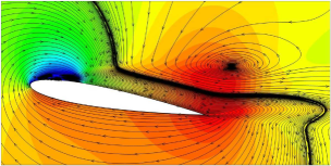
$\alpha=9.8^{\circ}$

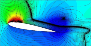
$\alpha=9.8^{\circ}$

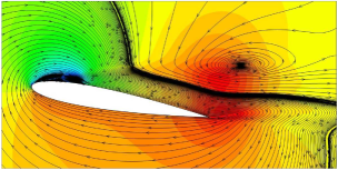
$\alpha=9.9^{\circ}$

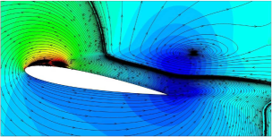
$\alpha=9.9^{\circ}$

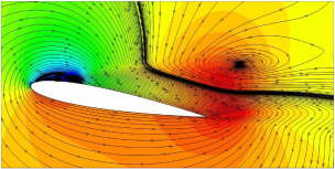
$\alpha=10.0^{\circ}$

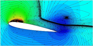
$\alpha=10.0^{\circ}$

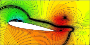
$\alpha=10.1^{\circ}$

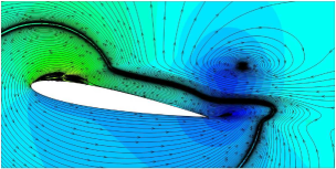
$\alpha=10.1^{\circ}$

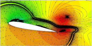
$\alpha=10.5^{\circ}$

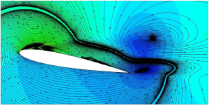
$\alpha=10.5^{\circ}$

Figure 3: Streamlines patterns of the time-averaged attached and separated phases of the oscillating-flow-field superimposed on colour maps of the time-averaged attached and separated phases of the oscillating-pressure-field for the angles of attack $\alpha=9.8^{\circ}$–$10.5^{\circ}$. Left: time-averaged attached-phase of the oscillating-flow-field estimated from the high-lift flow-field minus the mean-lift flow-field, $\Delta{\overline{U}}^{\mathrm{+}}$, $\Delta{\overline{V}}^{\mathrm{+}}$, and $\Delta{\overline{P}}^{\mathrm{+}}$. Right: time-averaged separated-phase of the oscillating-flow-field estimated from the low-lift flow-field minus the mean-lift flow-field, $\Delta{\overline{U}}^{\mathrm{-}}$, $\Delta{\overline{V}}^{\mathrm{-}}$, and $\Delta{\overline{P}}^{\mathrm{-}}$.

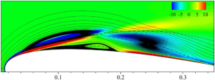
$\alpha=9.8^{\circ}$.

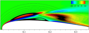
$\alpha=9.8^{\circ}$.

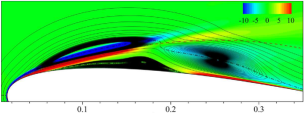
$\alpha=9.9^{\circ}$.

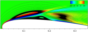
$\alpha=9.9^{\circ}$.

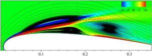
$\alpha=10.0^{\circ}$.

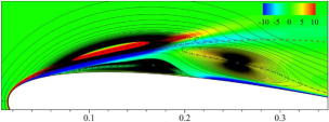
$\alpha=10.0^{\circ}$.

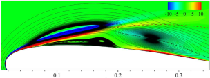
$\alpha=10.1^{\circ}$.

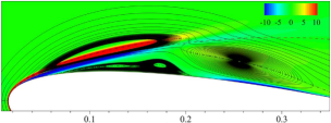
$\alpha=10.1^{\circ}$.

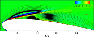
$\alpha=10.5^{\circ}$.

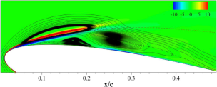
$\alpha=10.5^{\circ}$.

Figure 6: Streamlines patterns of the time-averaged attached and separated phases of the oscillating-flow-field superimposed on colour maps of the time-averaged attached and separated phases of the oscillating-spanwise-vorticity for the angles of attack $\alpha=9.8^{\circ}$–$10.5^{\circ}$. The red dashed line displays the streamline that bounds the LSB in the mean sense. The black dash-dot line denotes the contour line at which the time-average oscillating-streamwise-velocity equals zero. Left: time-average attached-phase of the oscillating-flow-field estimated from the high-lift flow minus the mean-lift flow-field, $\Delta{\overline{U}}^{\mathrm{+}}$ and $\Delta{\overline{V}}^{\mathrm{+}}$. Right: time-average separated-phase of the oscillating-flow estimated from the low-lift flow minus the mean-lift flow-field, $\Delta{\overline{U}}^{\mathrm{-}}$ and $\Delta{\overline{V}}^{\mathrm{-}}$.

$\alpha=9.25^{\circ}$

References

- Alam & Sandham (2000) Alam, M. & Sandham, N. D. 2000 Direct numerical simulation of “short” laminar separation bubbles with turbulent reattachment. Journal of Fluid Mechanics 403, 223–250.
- Almutairi & Alqadi (2013) Almutairi, J. & Alqadi, I. 2013 Large-eddy simulation of natural low-frequency oscillations of separating–reattaching flow near stall conditions. AIAA journal 51 (4), 981–991.
- Almutairi et al. (2015) Almutairi, J., Alqadi, I. & Eljack, E. 2015 Large eddy simulation of a naca-0012 airfoil near stall. In Fröhlich J., Kuerten H., Geurts B., Armenio V. (eds) Direct and Large-Eddy Simulation IX. ERCOFTAC Series, vol 20., pp. 389–395. Springer, Cham.
- Almutairi et al. (2010) Almutairi, J. H., Jones, L. E. & Sandham, N. D. 2010 Intermittent bursting of a laminar separation bubble on an airfoil. AIAA journal 48 (2), 414–426.
- Ansell & Bragg (2013) Ansell, P. J. & Bragg, M. B. 2013 Characterization of ice-induced low-frequency flowfield oscillations and their effect on airfoil performance. In 31 AIAA Applied Aerodynamics Conference, AIAA Paper 2013-2673 31. American Institute of Aeronautics and Astronautics.
- Ansell & Bragg (2015a) Ansell, P. J. & Bragg, M. B. 2015a Characterization of low-frequency oscillations in the flowfield about an iced airfoil. AIAA Journal 53 (3), 629–637.
- Ansell & Bragg (2015b) Ansell, P. J. & Bragg, M. B. 2015b Unsteady modes in flowfield about airfoil with horn-ice shape. Journal of Aircraft 53 (2), 475–486.
- Bragg et al. (1996) Bragg, M. B., Heinrich, D. C., Balow, F. A. & Zaman, K. B. M. Q. 1996 Flow oscillation over an airfoil near stall. AIAA journal 34 (1), 199–201.
- Bragg et al. (1993) Bragg, M. B., Heinrich, D. C & Khodadoust, A. 1993 Low-frequency flow oscillation over airfoils near stall. AIAA journal 31 (7), 1341–1343.
- Bragg et al. (1992) Bragg, M. B., Khodadoust, A. & Spring, S. A. 1992 Measurements in a leading-edge separation bubble due to a simulated airfoil ice accretion. AIAA journal 30 (6), 1462–1467.
- Broeren & Bragg (1998) Broeren, A. P. & Bragg, M. B. 1998 Low-frequency flowfield unsteadiness during airfoil stall and the influence of stall type. In 16 AIAA Applied Aerodynamics Conference, AIAA-98-2517 16, pp. 196–209.
- Broeren & Bragg (1999) Broeren, A. P. & Bragg, M. B. 1999 Flowfield measurements over an airfoil during natural low-frequency oscillations near stall. AIAA journal 37 (1), 130–132.
- Broeren & Bragg (2001) Broeren, Andy P & Bragg, Michael B 2001 Spanwise variation in the unsteady stalling flowfields of two-dimensional airfoil models. AIAA journal 39 (9), 1641–1651.
- Diwan & Chetan (2006) Diwan, S. S. & Chetan, S. J. 2006 ON THE BURSTING CRITERION FOR LAMINAR SEPARATION BUBBLES, pp. 401–407. Springer Netherlands.
- Diwan & Ramesh (2007) Diwan, S. S. & Ramesh, O. N. 2007 Laminar separation bubbles: Dynamics and control. Sadhana 32 (1), 103–109.
- Diwan & Ramesh (2009) Diwan, S. S. & Ramesh, O. N. 2009 On the origin of the inflectional instability of a laminar separation bubble. Journal of Fluid Mechanics 629, 263–298.
- Eljack (2017) Eljack, Eltayeb 2017 High-fidelity numerical simulation of the flow field around a naca-0012 aerofoil from the laminar separation bubble to a full stall. International Journal of Computational Fluid Dynamics 31 (4-5), 230–245.
- Eljack et al. (2018a) Eljack, E., Alqadi, I. & Almutairi, J. 2018a Influence of periodic forcing on laminar separation bubble. In Grigoriadis D., Geurts B., Kuerten H., Fröhlich J., Armenio V. (eds) Direct and Large-Eddy Simulation X. ERCOFTAC Series, vol 24., pp. 199–204. Springer, Cham.
- Eljack et al. (2018b) Eljack, E., Alqadi, I. & Soria, J. 2018b Bursting and reformation cycle of the laminar separation bubble over a naca-0012 aerofoil: Characterisation of the flow-field. ArXiv e-prints , arXiv: 1807.04573.
- Gaster (1963) Gaster, M. 1963 On the stability of parallel flows and the behaviour of separation bubbles. Phd thesis, Queen Mary College, University of London.
- Gaster (1967) Gaster, M. 1967 The structure and behaviour of laminar separation bubbles. HMSO.
- Häggmark et al. (2001) Häggmark, C. P., Hildings, C. & Henningson, D. S. 2001 A numerical and experimental study of a transitional separation bubble. Aerospace science and technology 5 (5), 317–328.
- Horton (1968) Horton, H. P. 1968 Laminar separation bubbles in two and three dimensional incompressible flow. Phd thesis, Queen Mary College, University of London.
- Jones et al. (2008) Jones, L. E., Sandberg, R. D. & Sandham, N. D. 2008 Direct numerical simulations of forced and unforced separation bubbles on an airfoil at incidence. Journal of Fluid Mechanics 602, 175–207.
- Jones et al. (2010) Jones, L. E., Sandberg, R. D. & Sandham, N. D. 2010 Stability and receptivity characteristics of a laminar separation bubble on an aerofoil. Journal of Fluid Mechanics 648, 257–296.
- Marxen (2008) Marxen, O. 2008 Laminar-turbulent transition in a laminar separation bubble: Influence of disturbance amplitude on bubble size and bursting. In High Performance Computing in Science and Engineering07, pp. 261–275. Springer.
- Marxen & Henningson (2007) Marxen, O. & Henningson, D. 2007 Numerical simulation of the bursting of a laminar separation bubble. In High Performance Computing in Science and Engineering 06, pp. 253–267. Springer.
- Marxen & Henningson (2008) Marxen, O. & Henningson, D. 2008 Direct numerical simulation of a short laminar separation bubble and early stages of the bursting process. In New Results in Numerical and Experimental Fluid Mechanics VI, pp. 235–243. Springer.
- Marxen & Henningson (2011) Marxen, O. & Henningson, D. S. 2011 The effect of small-amplitude convective disturbances on the size and bursting of a laminar separation bubble. Journal of Fluid Mechanics 671, 1–33.
- Marxen et al. (2013) Marxen, O., Lang, M. & Rist, U. 2013 Vortex formation and vortex breakup in a laminar separation bubble. Journal of Fluid Mechanics 728, 58–90.
- Marxen et al. (2003) Marxen, O., Lang, M., Rist, U. & Wagner, S. 2003 A combined experimental/numerical study of unsteady phenomena in a laminar separation bubble. Flow, Turbulence and Combustion 71 (1-4), 133–146.
- Marxen & Rist (2010) Marxen, O. & Rist, U. 2010 Mean flow deformation in a laminar separation bubble: separation and stability characteristics. Journal of Fluid Mechanics 660, 37–54.
- Marxen et al. (2007) Marxen, O., You, D. & Moin, P. 2007 Numerical simulations of the bursting of a laminar separation bubble and its relation to airfoil stall. In Advances in Turbulence XI, pp. 712–714. Springer.
- Maucher et al. (2000) Maucher, U., Rist, U., Kloker, M. & Wagner, S. 2000 Dns of laminar-turbulent transition in separation bubbles. In High Performance Computing in Science and Engineering 99, pp. 279–294. Springer.
- Maucher et al. (1994) Maucher, U., Rist, U. & Wagner, S. 1994 Direct numerical simulation of airfoil separation bubbles. In Computational Fluid Dynamics 94, pp. 471–477.
- McGregor (1954) McGregor, I. 1954 Regions of localised boundary layer separation and their role in nose stalling of aerofoils. Phd thesis, Queen Mary College, University of London.
- Rinoie & Takemura (2004) Rinoie, K. & Takemura, N. 2004 Oscillating behaviour of laminar separation bubble formed on an aerofoil near stall. Aeronautical Journal 108 (1081), 153–163.
- Rist (2002) Rist, U. 2002 On instabilities and transition in laminar separation bubbles. In Proc CEAS aerospace aerodynamics research conference, pp. 10–12.
- Rist (2003) Rist, U. 2003 Instability and transition mechanisms in laminar separation bubbles. Von Kármán Institute Lecture Series .
- Rist & Maucher (2002) Rist, U. & Maucher, U. 2002 Investigations of time-growing instabilities in laminar separation bubbles. European Journal of Mechanics-B/Fluids 21 (5), 495–509.
- Rodríguez et al. (2015) Rodríguez, I., Lehmkuhl, O., Borrell, R. & A., Oliva 2015 Flow past a naca0012 airfoil: From laminar separation bubbles to fully stalled regime. In Fröhlich J., Kuerten H., Geurts B., Armenio V. (eds) Direct and Large-Eddy Simulation IX. ERCOFTAC Series, vol 20., pp. 225–231. Springer, Cham.
- Rodríguez et al. (2013) Rodríguez, I., Lehmkuhl, O., Borrell, R. & Oliva, A. 2013 Direct numerical simulation of a naca0012 in full stall. International Journal of Heat and Fluid Flow 43 (Supplement C), 194–203, 7th International Symposium on Turbulence Heat & Mass Transfer (THMT-7), Palermo Conference on Modelling Fluid Flow (CMFF 12).
- Sandham (2008) Sandham, N. D. 2008 Transitional separation bubbles and unsteady aspects of aerofoil stall. Aeronautical Journal 112 (1133), 395–404.
- Tanaka (2004) Tanaka, H. 2004 Flow visualization and piv measurements of laminar separation bubble oscillating at low frequency on an airfoil near stall. In International Congress of the Aeronautical Sciences.
- Woodward (1970) Woodward, D. S. 1970 An investigation of the flow in separation bubbles. Phd thesis, Queen Mary College, University of London.
- Zaman (1992) Zaman, K. B. M. Q. 1992 Effect of acoustic excitation on stalled flows over an airfoil. AIAA journal 30 (6), 1492–1499.
- Zaman et al. (1987) Zaman, K. B. M. Q., Bar-Sever, A. & Mangalam, S. M. 1987 Effect of acoustic excitation on the flow over a low-re airfoil. Journal of Fluid Mechanics 182, 127–148.
- Zaman & McKinzie (1988) Zaman, K. B. M. Q. & McKinzie, D. J. 1988 A natural low frequency oscillation in the wake of an airfoil near stalling conditions. Tech. Rep. NASA/TM-100213. Lewis Research Center.
- Zaman & McKinzie (1991) Zaman, K. B. M. Q. & McKinzie, D. J. 1991 Control of laminar separation over airfoils by acoustic excitation. AIAA journal 29 (7), 1075–1083.
- Zaman et al. (1989) Zaman, K. B. M. Q., McKinzie, D. J. & Rumsey, C. L. 1989 A natural low-frequency oscillation of the flow over an airfoil near stalling conditions. Journal of Fluid Mechanics 202, 403–442.
- Zaman & Potapczuk (1989) Zaman, K. B. M. Q. & Potapczuk, M. G. 1989 The low frequency oscillation in the flow over a naca0012 airfoil with an “iced” leading edge. Tech. Rep. NASA TM-102018. Lewis Research Center.