Strain dependence of photoluminescence and circular dichroism in transition metal dichalcogenides: a k • p analysis

Abstract

Within a two-band $k\cdot p$ method we analyze different types of strain for the $K$ valley optical characteristics of a freestanding monolayer MoS₂, MoSe₂, WS₂ and WSe₂. We predict that circular polarization selectivity for energies above the direct transition onset deteriorates/improves by tensile/compressive strain. Wide range of available strained-sample photoluminescence data can be reasonably reproduced by this simple bandstructure combined with accounting for excitons at a variational level. According to this model strain impacts optoelectronic properties through its hydrostatic component, whereas the shear strain only causes a rigid wavevector shift of the valley. Furthermore, under the stress loading of flexible substrates the presence of Poisson’s effect or the lack of it are examined individually for the reported measurements.

1 Introduction

Transition metal dichalcogenides (TMDs) possess direct optical gap together with mechanical flexibility up to 10% range [1] which enables wide strain tunability of their optoelectronic properties [2, 3]. As a consequence, the associated body of literature is rapidly growing, while a number of milestones have been reached. The tuning of the electronic structure by applying a uniaxial tensile bending to monolayer MoS₂ on flexible substrates has been demonstrated by several groups within a short time span [4, 5, 6, 7, 8, 9, 10]. For a suspended monolayer MoS₂ membrane, Lloyd et al. showed the continuous and reversible tuning of the optical bandgap over an ultralarge range of applied biaxial strain [11]. More recently, deterministic two-dimensional array of quantum emitters from thin TMDs due to a localized strain pattern is achieved that becomes instrumental to construct scalable quantum architectures [12, 13]. Additional experimental [14, 15, 16, 17, 18, 19, 20, 21] as well as theoretical [22, 23, 24, 25] studies substantiated strain as a viable control mechanism for these two-dimensional materials.

Our aim in this work is to consolidate accumulating experimental photoluminescence (PL) data on strained TMD samples with the aid of a simple $K$-valley-specific two-band $k\cdot p$ theory. Particularly, for the measurements performed by uniaxial bending of flexible substrates, this analysis can reveal the extend of Poisson’s contraction over the TMD layer for each individual case. It also governs the circular dichroism which refers to the helicity-selective optical absorption [26], and in which way it can be altered by strain.

2 Theory

2.1 Two-band strained $k\cdot p$ approach for TMDs

The conduction and valence bands of TMDs around the direct bandgap at the $K_{\pm}$ valleys can be represented by a two-band basis $\left\{\Ket{\phi_{c}},\Ket{\phi^{\pm}_{v}}\right\}$ which primarily accounts for the $d$-orbitals, $\Ket{d_{z^{2}}}$ and $\left(\Ket{d_{x^{2}-y^{2}}}\pm i\Ket{d_{xy}}\right)/\sqrt{2}$ [27]. The corresponding strained $k\cdot p$ Hamiltonian has been very recently suggested by Fang et al., which in this basis attains the matrix form

$$H=\left[\begin{array}[]{cc}\left(f_{0}+\frac{f_{1}}{2}\right)+(f_{3}+f_{4})(\varepsilon_{xx}+\varepsilon_{yy})&f_{2}a(k_{x}-ik_{y})+f_{5}(\varepsilon_{xx}-\varepsilon_{yy}+2i\varepsilon_{xy})\\ f_{2}a(k_{x}+ik_{y})+f_{5}(\varepsilon_{xx}-\varepsilon_{yy}-2i\varepsilon_{xy})&\left(f_{0}-\frac{f_{1}}{2}\right)+(f_{3}-f_{4})(\varepsilon_{xx}+\varepsilon_{yy})\end{array}\right]\,,$$ (1)

where $a$ is the lattice constant, $f_{i}$’s are the strained $k\cdot p$ parameters fitted to first-principles electronic bandstructure, also listed in Table 1 for convenience [28]. Among these six $k\cdot p$ parameters, $f_{0}$ and $f_{3}$ do not play a role in homogeneous systems (as in this work). Their significance emerges in vertical heterostructures [29] for $f_{0}$, and in localized strain gradients [12, 13] for $f_{3}$. In Eq. (1) as well as in the remainder of this work, without loss of generality we refer to $K_{+}$ valley, which is assumed to be the origin for the wavevector $\vec{k}=\hat{x}k_{x}+\hat{y}k_{y}$, where $\hat{x}$ points from $\Gamma$ to $K_{+}$ in reciprocal space, that matches with the “zigzag” direction in direct space. Expressions for the $K_{-}$ valley, if required, can be obtained by complex conjugation, as the $K_{\pm}$ points are connected through time-reversal symmetry [30]. The spin and the spin-orbit coupling are discarded in Eq. (1), although the spin-splitting can be easily incorporated to this framework [28]. For our purposes this is not necessary as we are interested in the so-called $A$-excitons only [5].

Table 1: $k.p$ parameters $f_{i}$ (eV), lattice constant $a$ (Å) [28], 2D polarizability $\chi_{\textit{2D}}$ (Å)[31] for different TMDs.

Materials	$f_{0}$	$f_{1}$	$f_{2}$	$f_{3}$	$f_{4}$	$f_{5}$	$a$	$\chi_{\textit{2D}}$
MoS2	-5.07	1.79	1.06	-5.47	-2.59	2.2	3.182	6.60
MoSe2	-4.59	1.55	0.88	-5.01	-2.28	1.84	3.317	8.23
WS2	-4.66	1.95	1.22	-5.82	-3.59	2.27	3.182	6.03
WSe2	-4.23	1.65	1.02	-5.26	-3.02	2.03	3.316	7.18

Neglecting any displacement perpendicular to TMD that lies on the two-dimensional (2D) $xy$-plane, the tensor strain components for most common types are:

$$\mathrm{Biaxial~{}strain:} \varepsilon_{yy}=\varepsilon_{xx},~{}~{}~{}\varepsilon_{xy}=\varepsilon_{yx}=0,$$

$$\mathrm{Uniaxial~{}strain:} \varepsilon_{xx}\neq 0,~{}~{}~{}\varepsilon_{yy}=\varepsilon_{xy}=\varepsilon_{yx}=0,$$

$$\mathrm{Shear~{}strain:} \varepsilon_{yy}=-\varepsilon_{xx},~{}~{}~{}\varepsilon_{xy}=\varepsilon_{yx}\neq 0,$$

$$\mathrm{Uniaxial~{}stress:} \varepsilon_{yy}=-\nu\varepsilon_{xx},~{}~{}~{}\varepsilon_{xy}=\varepsilon_{yx}=0,$$

where $\nu$ is the Poisson’s ratio. To simplify our expressions, also we make use of the (areal) hydrostatic component of strain, $\varepsilon_{H}=\varepsilon_{xx}+\varepsilon_{yy}$. Regarding the terminology, we should caution that the term uniaxial strain is in widespread use in TMD literature [5, 3, 20, 21], although with the assumed Poisson’s effect, as explicitly mentioned in these works, it needs to be referred to as uniaxial stress; also note that we use tensor and not the engineering strain [32].

The strained eigenstates of Eq. (1) can be readily solved analytically. The direct bandgap becomes $E_{g}=f_{1}+2f_{4}\varepsilon_{H}$. If we introduce $k_{x0}\equiv(\varepsilon_{xx}-\varepsilon_{yy})f_{5}/(f_{2}a)$, $k_{y0}\equiv 2\varepsilon_{xy}f_{5}/(f_{2}a)$, and $q_{x}\equiv k_{x}-k_{x0}$, $q_{y}\equiv k_{y}-k_{y0}$, with their magnitude $q=\sqrt{q_{x}^{2}+q_{y}^{2}}$, the energy dispersion for the conduction and valence bands can be expressed as

$$E_{c/v}(q)=f_{0}+f_{3}\varepsilon_{H}\pm\frac{E_{g}}{2}\sqrt{1+4\left[r(q,\varepsilon_{H})\right]^{2}},$$ (2)

in terms of an auxiliary function that depends on the (valley edge-centered) wavenumber and the hydrostatic strain as

$$r(q,\varepsilon_{H})\equiv\frac{f_{2}aq}{f_{1}+2f_{4}\varepsilon_{H}},$$ (3)

which quantifies the degree of mixing between basis states $\left\{\Ket{\phi_{c}},\Ket{\phi_{v}}\right\}$ as to be justified below.

Hence, the valley edge shifts from $(k_{x}=0,k_{y}=0)$ to $(k_{x0},k_{y0})$ because of strain. So that for $\varepsilon_{xx}>\varepsilon_{yy}$, $k_{x0}>0$, and band extremum at $K$ shifts away from $\Gamma$ (toward neighboring zone $M^{\prime}$) point, while for $\varepsilon_{yy}>\varepsilon_{xx}$, $k_{x0}<0$ it shifts toward $\Gamma$ point. Thus, according to this simple model the shear strain rigidly displaces it along $k_{y}$ direction without affecting the bandgap. As a matter of fact the terms proportional to $f_{5}$ in Eq. (1) were referred to as the pseudogauge field in the graphene literature, responsible for shifting the Dirac cone from the $K$ point [28].

The eigenvectors of the two-band Hamiltonian in Eq. (1) corresponding to the conduction and valence states are given by

$$\ket{U_{c}}=\left(\begin{array}[]{c}x_{1}\\ x_{2}\end{array}\right),~{}~{}~{}\ket{U_{v}}=\left(\begin{array}[]{c}x_{2}\\ -x_{1}^{*}\end{array}\right)\,,$$ (4)

where in terms of $\phi=\tan^{-1}(q_{y}/q_{x})$, an $r$ defined in Eq. (3) the entries are given by

$$x_{1} = \frac{e^{-i\phi}}{\sqrt{1+r^{2}}},$$ (5)

$$x_{2} = \frac{r}{\sqrt{1+r^{2}}}.$$ (6)

2.2 Degree of circular polarization

For a light polarized along a unit vector $\hat{u}$, the dipole matrix element connecting valence $\ket{U_{v}}$ and conduction $\ket{U_{c}}$ states is given by [27]

$$\mathcal{P}_{u}(\vec{k})\equiv\frac{m_{0}}{\hbar}\bra{U_{c}}\frac{\partial\hat{H}}{\partial k_{u}}\ket{U_{v}}\,,$$ (7)

where $m_{0}$ is the free electron mass. For the $\pm$ circularly polarized light defined by the unit vectors $\hat{u}_{\pm}=\left(\hat{x}\pm i\hat{y}\right)/\sqrt{2}$, Eq. (7) can be expressed in terms of Pauli spin raising/lowering operators $\hat{\sigma}_{\pm}$ as

$$\mathcal{P}_{\pm}(\vec{k})=\frac{m_{0}f_{2}a}{\sqrt{2}\hbar}\braket{U_{c}}{\hat{\sigma}_{\pm}}{U_{v}}.$$ (8)

Though it is not directly apparent from this expression, these momentum matrix elements are actually strain dependent through the eigenkets in Eq. (4) and the mixing function $r(q,\varepsilon_{H})$ from Eq. (3).

The so-called circular dichroism (CD) corresponds to a difference in the absorption of the right- and left-hand circularly polarized radiation, where the $k-$resolved degree of helicity selectivity is quantified as [26],

$$\eta(\vec{k})\equiv\frac{|\mathcal{P}_{+}(\vec{k})|^{2}-|\mathcal{P}_{-}(\vec{k})|^{2}}{|\mathcal{P}_{+}(\vec{k})|^{2}+|\mathcal{P}_{-}(\vec{k})|^{2}}\,.$$ (9)

We should note that inclusion of spin and the spin-orbit coupling does not affect the above helicity selection rules [33]. For isotropic and electron-hole symmetric bands as in our case, its wavevector dependence simplifies as $\eta(\vec{k})\rightarrow\eta(q)=\eta(E)$. By inserting the associated states from Eq. (4) it acquires a simple analytical form

$$\eta(q,\varepsilon_{H})=\frac{1-\left[r(q,\varepsilon_{H})\right]^{4}}{1+\left[r(q,\varepsilon_{H})\right]^{4}},$$ (10)

in terms of $r(q,\varepsilon_{H})$ defined in Eq. (3).

2.3 Exciton binding and PL energies

To compare with the experimental PL data under a given strain, we need to include excitonic effects as the associated binding energies significantly exceed the thermal energy at room temperature [5]. For that, we first extract the valley edge effective masses $m_{c/v}^{*}$ from the energy dispersion relation (Eq. (2)) via,

$$m_{c/v}^{*}=\frac{\hbar^{2}}{\left(\left.\frac{\partial^{2}E_{c/v}}{\partial k^{2}}\right|_{k_{x0},k_{y0}}\right)}=\pm\frac{\hbar^{2}\left(f_{1}+2f_{4}\varepsilon_{H}\right)}{2(f_{2}a)^{2}}\,,$$ (11)

where the curvatures are evaluated at the strained band extremum, $(k_{x0},k_{y0})$. Within our two-band $k\cdot p$ model electron and hole effective masses are equal, i.e., $m^{*}_{e}=m^{*}_{c}=m^{*}_{h}=-m^{*}_{v}$, and furthermore they are spatially isotropic, but note that here these effective masses are strain-dependent. Thus, the corresponding exciton effective mass for its relative degrees of freedom follows from $\mu=m^{*}_{e}m^{*}_{h}/\left(m^{*}_{e}+m^{*}_{h}\right)$.

To retain the simplicity of our approach, the binding energies for neutral excitons in TMDs can be calculated following [31] by a variational method based on the exciton Hamiltonian (switching to Hartree atomic units in the remainder of this subsection),

$$H_{X}=-\frac{\nabla_{\textit{2D}}^{2}}{2\mu}+V_{\textit{2D}}(\rho)\,.$$ (12)

Here, the in-plane interaction between an electron and a hole separated by $\rho=\sqrt{x^{2}+y^{2}}$ is,

$$V_{\textit{2D}}(\rho)=\frac{-\pi}{(\kappa_{a}+\kappa_{b})\rho_{0}}\left[H_{0}(\rho/\rho_{0})-Y_{0}(\rho/\rho_{0})\right],$$ (13)

where, $\kappa_{a}$ and $\kappa_{b}$ are dielectric constants for the media above and below the TMD (for a freestanding case, $\kappa_{a}=\kappa_{b}=1$), $H_{0}$ and $Y_{0}$ are the Struve and the Bessel function of the second kind; the screening length is given by $\rho_{0}=2\pi\chi_{\textit{2D}}$, and $\chi_{\textit{2D}}$ is the 2D polarizability of the TMD, which is listed in Table 1 [31].

The wave function for the neutral exciton with a single variational parameter $\lambda$ is chosen as,

$$\Psi_{X}(\rho;\lambda)=\sqrt{\frac{2}{\pi\lambda^{2}}}\exp{(-\rho/\lambda)}.$$ (14)

In such a case the kinetic energy has the analytical form, $T(\lambda)=1/(2\mu\lambda^{2}),$ while potential energy requires the following integration to be evaluated numerically,

$$V(\lambda)=-\frac{2\pi}{\rho_{0}\lambda^{2}}\int_{0}^{\infty}[H_{0}(\rho/\rho_{0})-Y_{0}(\rho/\rho_{0})]~{}\exp{(-2\rho/\lambda)}~{}\rho~{}d\rho.$$ (15)

The total exciton energy is found by minimizing $E_{X}(\lambda)=T(\lambda)+V(\lambda)$, where the optimum value of $\lambda$ corresponds to the mean the exciton radius. For a bound exciton $E_{X}<0$, and the PL energy is obtained from $E_{\textit{PL}}=E_{g}+E_{X}$.

2.4 A critique of the two-band Hamiltonian

The Hamiltonian of Eq. (1) was originally derived from a simplified tight binding model for TMDs [34]. Alternatively, starting from the well-known unstrained $k\cdot p$ model [27], it can be arrived through the substitutions

$$k_{x}\rightarrow k_{x}+\alpha\left(\varepsilon_{yy}-\varepsilon_{xx}\right)\,,~{}~{}~{}k_{y}\rightarrow k_{y}+\alpha 2\varepsilon_{xy}\,,$$ (16)

that resembles a minimal coupling to a strain-related gauge field with a coupling constant $\alpha$ (which is $f_{5}$ in our case) [35]. A group-theoretic basis of this substitution is that for the $C_{3h}$ point symmetry of the $K$ point in TMDs, both $k_{x}-ik_{y}$ and $\left(\varepsilon_{xx}-\varepsilon_{yy}\right)+i2\varepsilon_{xy}$ transform according to $K_{2}$ ($\Gamma_{3}$ in the notation of [36]), while $k_{x}+ik_{y}$ and $\left(\varepsilon_{xx}-\varepsilon_{yy}\right)-i2\varepsilon_{xy}$ transform according to $K_{3}$ ($\Gamma_{2}$) irreducible representations [37]. Moreover, both $\Gamma_{2}$ and $\Gamma_{3}$ transform the same way under time-reversal symmetry [36].

Even though the substitution recipe in Eq. (16) when applied to the unstrained Hamiltonian of [27] generates strain terms respecting the symmetry of $K$ point, it fails to produce higher-order strain effects. The rigorous approach following the method of invariants [38] allows additional terms, like for instance, $\left(\varepsilon_{yy}-\varepsilon_{xx}\right)k_{x}+2\varepsilon_{xy}k_{y}$ on the diagonal entries of Eq. (1) [35]. Unfortunately, at the present their coupling constants, similar to those in Table 1 are unavailable. In the absence of such terms, strain can only affect the dispersion via a single parameter $f_{4}$ (see, Eqs. (2) and (3)) which amounts to a significant reduction in the degrees of freedom. As such, it is the underlying reason for the retention of isotropy of effective masses under the uniaxial deformation, which can be inferred from Eq. (2) by the circular isoenergy curves for this case. However, from a quantitative point of view we believe that the implicit electron-hole symmetry from Eq. (11) is more of a concern that equates their effective masses; and yet, there exist other missing terms such as trigonal warping, and a cubic deviation in the band structure [30].

3 Results and discussions

3.1 Effect of strain on circular dichroism

In pristine TMDs the CD stems from two crystal properties, namely the lack of center of inversion and the existance of the threefold rotational point symmetry, $C_{3}$ [26]. At the $K_{\pm}$ point (i.e., $q=0$) CD is maximum ($\eta=1$) that strictly allows the $\sigma^{+}$ ($\sigma^{-}$) helicity across the $K_{+}$ ($K_{-}$) direct transition between the two-band basis states of $\Ket{\phi_{c}}$ and $\Ket{\phi^{\pm}_{v}}$. Away from the $K$ point, the conduction and valence states develop an admixture of these basis states that leads to a degradation in the helicity discrimination, and hence in $\eta$. This can be mathematically followed from Eq. (4), where an increase in $q$ causes a mixing of the valley edge ($q=0$) states as mediated by the $r$ function (see, Eq. (3)).

To illustrate how strain affects this situation, using Eq. (9) we plot in Fig. 1 $\eta(\Delta E)$ for various excess energies defined as $\Delta E=(E-E_{g})/2$, where $E$ is the energy of the incoming photon. The presence of a hydrostatic strain component $\varepsilon_{H}$ either enhances or diminishes the variation in the mixing function $r$ and hence $\eta$ depending on the overall sign of $f_{4}\varepsilon_{H}$. With $f_{4}<0$ as seen from Table 1, this explains why the tensile strain $\varepsilon_{H}>0$ ($\varepsilon_{xx}>0$ in Fig. 1) inflates the variation in $\eta$ in Fig. 1. We also observe that selenium-TMDs are more sensitive to strain in this respect, and the amount of change is larger for biaxial than uniaxial strain, as expected, for all of these materials.

The above CD analysis is rather simplistic for a number of reasons. It does not include the excitonic interaction which would average $\eta(k)$ in a region of the $k$-space over which the exciton wave function extends. A more subtle consequence of the long range Coulomb interaction between the electron and the hole is that it acts as an effective magnetic field causing the coupling of $\sigma^{\pm}$ polarizations of the exciton that results in linearly polarized longitudinal and transverse eigenstates, and hence in the so-called linear dichroism [39, 33, 40]. This is also left out of the scope of this work. Finally, any intervalley scattering [41, 42, 43] or other processes [44] not considered here will further impair the CD.

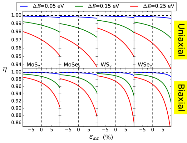
Figure 1: Effect of uniaxial/biaxial strain on the degree of optical polarization of TMDs for compressive/tensile strain at different excess energies $\Delta E$, as measured from the conduction band minimum.

3.2 PL peak shift under strain

Figure 2 shows the PL peak shift for the four TMDs under uniaxial strain, comparing our calculations with the data from numerous experimental references. For MoS₂ and WSe₂ we have a good agreement between our theory and the best fit to the experimental data, taking into account the spread in the latter. At variance to this, for WS₂ our results do not agree with two reports [18, 19]. To resolve this case, we also plot the bandgap variation for WS₂ under uniaxial strain from a first-principles calculation [24] (yellow-dashed). If we add to this the strained excitonic correction we get a closer agreement with our calculations (purple-dotted vs. blue-solid). Therefore, we believe that some slipping may have occured on the TMD layer while applying strain to the substrate in [18, 19], whereas other measurements in Fig. 2 such as [5, 20, 21] have taken measures to clamp the TMD to the substrate. For MoSe₂, we see that the uniaxial stress condition using the Poisson’s ratio of the substrate, $\nu=0.37$ (blue-dashed) matches perfectly with the data, in agreement with their assertion in [21]. In other words, unlike the other measurements in Fig. 2, for this experiment the TMD layer fully complies with the Poisson’s contraction of the substrate.

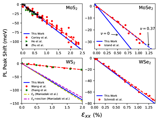
Figure 2: Uniaxial strain dependence of $A$-exciton PL peak energy shift for monolayer TMDs, comparing our calculations (in blue) with experimental data (symbols) along with their best fit line (red-dashed). References: Conley et al. [5], Island et al. [21], Wang et al. [18], Zhang et al. [19], Schmidt et al. [20], Maniadaki et al. [24].

Table 2: PL peak redshift under uniaxial or biaxial strain in comparison with results from literature. Our results (this work) have both uniaxial strain/stress (i.e., $\nu:~{}$0/0.37) cases with the values in parentheses corresponding those without the excitonic contribution.

meV${/\%}$	MoS2		MoSe2		WS2		WSe2
	Uniaxial	Biaxial	Uniaxial	Biaxial	Uniaxial	Biaxial	Uniaxial	Biaxial
This Work	49.4/31.1 (51.8/32.6)	98.8 (103.6)	43.6/27.5 (45.6/28.7)	87.2 (91.2)	68.5/43.2 (71.8/45.2)	137 (143.6)	57.6/36.3 (60.4/38.1)	115.2 (120.8)
Literature	$\sim$45a, $\sim$70b, $\sim$48c	99$\pm$6d, (90.15), 90.1e	27$\pm$2f	53.74e	11.3g, 10h	157e	54i	111e

References: ^a [5], ^b [4], ^c [6], ^d [11], ^e [45], ^f [21], ^g [18], ^h [19], ⁱ [20]

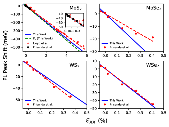
Figure 3: Biaxial strain dependence of $A$-exciton PL peak energy shift for monolayer TMDs, comparing our calculations (blue-solid) with experimental data (symbols) along with their best fit line (red-dashed). References: Lloyd et al. [11], Frisenda et al. [45].

In the case of biaxial strain displayed in Fig. 3, for MoS₂ we have an excellent agreement with the widest-range strain data by Lloyd et al. [11] which goes up to 6%. Once again we plot the variation in the bandgap (green-dashed in upper-left panel); the notable offset from PL line indicates the extend of excitonic contribution on the strain variation of the PL energy. Here, our results as well as [11] are for freestanding monolayer TMDs, on the other hand the remaining biaxial strain data from [45] was originally reported with respect to polypropylene substrate strain. Therefore, to convert substrate strain results in [45], we multiplied all strain data from this reference by the $0.573$ scale factor. This brings their data in agreement with the freestanding case of [11]. However, for MoSe₂ we still have a disagreement with [45]; noting the leveling off in their data beyond about 0.15% strain, we again suspect that a slipping might be responsible.

In Table 2 we compare our PL peak strain shift results with the quantities from various experimental references. For our results, both uniaxial strain and uniaxial stress cases are presented, where in the former no transverse contraction takes place in the direction perpendicular to axial deformation (i.e., $\nu=0$). For uniaxial stress we use $\nu=0.37$ value which is typical for the flexible substrates in use [20, 21]. As mentioned above, the uniaxial stress condition applies only for the MoSe₂ experiment of [21]. We also quote in parentheses our results excluding the variation of exciton binding energy under strain. It can be observed that sulfur-TMDs are more responsive to strain for PL peak shift and the amount of change is larger for biaxial strain than uniaxial one for each material considered.

4 Conclusions

A simple two-band $k\cdot p$ approach within minimal coupling to strain as applied to TMDs shows that the bandgap and effective masses are affected by the hydrostatic component of the strain, whereas the shear strain does not alter the optoelectronic properties, but merely shifts the wavevector of the valley extrema. A mixing of the valley edge states occurs away from the extrema which is either amplified or diminished depending on the tensile or compressive nature of strain, respectively. This also manifests itself on the CD that can be tuned in either direction by applying tensile or compressive strain which is more pronounced for the biaxial case. Comparison of strain-dependent PL peak shifts with a wide range of experimental data for monolayer TMDs demonstrates a satisfactory agreement provided that excitonic effects are included, and it reveals whether Poisson’s effect takes place in a certain experiment. This analysis can easily be extended to other TMDs with the availability of their $k\cdot p$ parameters. It can also act as a benchmark for more refined theories.

References

- [1] S. Bertolazzi, J. Brivio, and A. Kis, “Stretching and breaking of ultrathin MoS2,” ACS Nano 5, 9703–9709 (2011).
- [2] D. Akinwande, N. Petrone, and J. Hone, “Two-dimensional flexible nanoelectronics,” Nat. Commun. 5, 5678 (2014).
- [3] R. Roldán, A. Castellanos-Gomez, E. Cappelluti, and F. Guinea, “Strain engineering in semiconducting two-dimensional crystals,” J. Phys. :Condens. Matter 27, 313201 (2015).
- [4] K. He, C. Poole, K. F. Mak, and J. Shan, “Experimental demonstration of continuous electronic structure tuning via strain in atomically thin MoS2,” Nano Lett. 13, 2931–2936 (2013).
- [5] H. J. Conley, B. Wang, J. I. Ziegler, R. F. Haglund, S. T. Pantelides, and K. I. Bolotin, “Bandgap engineering of strained monolayer and bilayer MoS2,” Nano Lett. 13, 3626–3630 (2013).
- [6] C. R. Zhu, G. Wang, B. L. Liu, X. Marie, X. F. Qiao, X. Zhang, X. X. Wu, H. Fan, P. H. Tan, T. Amand, and B. Urbaszek, “Strain tuning of optical emission energy and polarization in monolayer and bilayer MoS2,” Phys. Rev. B 88, 121301 (2013).
- [7] A. Castellanos-Gomez, R. Roldán, E. Cappelluti, M. Buscema, F. Guinea, H. S. J. van der Zant, and G. A. Steele, “Local strain engineering in atomically thin MoS2,” Nano Lett. 13, 5361–5366 (2013).
- [8] P. Tonndorf, R. Schmidt, P. Böttger, X. Zhang, J. Börner, A. Liebig, M. Albrecht, C. Kloc, O. Gordan, D. R. T. Zahn, S. M. de Vasconcellos, and R. Bratschitsch, “Photoluminescence emission and raman response of monolayer MoS2, MoSe2, and WSe2,” Opt. Express 21, 4908–4916 (2013).
- [9] Y. Y. Hui, X. Liu, W. Jie, N. Y. Chan, J. Hao, Y.-T. Hsu, L.-J. Li, W. Guo, and S. P. Lau, “Exceptional tunability of band energy in a compressively strained trilayer MoS2 sheet,” ACS Nano 7, 7126–7131 (2013).
- [10] D. Sercombe, S. Schwarz, O. Del Pozo-Zamudio, F. Liu, B. J. Robinson, E. A. Chekhovich, I. I. Tartakovskii, O. Kolosov, and A. I. Tartakovskii, “Optical investigation of the natural electron doping in thin MoS2 films deposited on dielectric substrates,” Sci. Rep. 3, 3489 (2013).
- [11] D. Lloyd, X. Liu, J. W. Christopher, L. Cantley, A. Wadehra, B. L. Kim, B. B. Goldberg, A. K. Swan, and J. S. Bunch, “Band gap engineering with ultralarge biaxial strains in suspended monolayer MoS2,” Nano Lett. 16, 5836–5841 (2016).
- [12] A. Branny, G. Wang, S. Kumar, C. Robert, B. Lassagne, X. Marie, B. D. Gerardot, and B. Urbaszek, “Discrete quantum dot like emitters in monolayer MoSe2: Spatial mapping, magneto-optics, and charge tuning,” Appl. Phys. Lett. 108, 142101 (2016).
- [13] C. Palacios-Berraquero, D. M. Kara, A. R.-P. Montblanch, M. Barbone, P. Latawiec, D. Yoon, A. K. Ott, M. Loncar, A. C. Ferrari, and M. Atatüre, “Large-scale quantum-emitter arrays in atomically thin semiconductors,” Nat. Commun. 8, 15093 (2017).
- [14] G. Plechinger, A. Castellanos-Gomez, M. Buscema, H. S. J. v. d. Zant, G. A. Steele, A. Kuc, T. Heine, C. Schüller, and T. Korn, “Control of biaxial strain in single-layer molybdenite using local thermal expansion of the substrate,” 2D Mater. 2, 015006 (2015).
- [15] H. Li, A. W. Contryman, X. Qian, S. M. Ardakani, Y. Gong, X. Wang, J. M. Weisse, C. H. Lee, J. Zhao, P. M. Ajayan, J. Li, H. C. Manoharan, and X. Zheng, “Optoelectronic crystal of artificial atoms in strain-textured molybdenum disulphide,” Nat. Commun. 6, 7381 (2015).
- [16] S. B. Desai, G. Seol, J. S. Kang, H. Fang, C. Battaglia, R. Kapadia, J. W. Ager, J. Guo, and A. Javey, “Strain-induced indirect to direct bandgap transition in multilayer WSe2,” Nano Lett. 14, 4592–4597 (2014).
- [17] S. Yang, C. Wang, H. Sahin, H. Chen, Y. Li, S.-S. Li, A. Suslu, F. M. Peeters, Q. Liu, J. Li, and S. Tongay, “Tuning the optical, magnetic, and electrical properties of ReSe2 by nanoscale strain engineering,” Nano Lett. 15, 1660–1666 (2015).
- [18] Y. Wang, C. Cong, W. Yang, J. Shang, N. Peimyoo, Y. Chen, J. Kang, J. Wang, W. Huang, and T. Yu, “Strain-induced direct-indirect bandgap transition and phonon modulation in monolayer WS2,” Nano Res. 8, 2562–2572 (2015).
- [19] Q. Zhang, Z. Chang, G. Xu, Z. Wang, Y. Zhang, Z.-Q. Xu, S. Chen, Q. Bao, J. Z. Liu, Y.-W. Mai et al., “Strain relaxation of monolayer WS2 on plastic substrate,” Adv. Funct. Mater. 26, 8707–8714 (2016).
- [20] R. Schmidt, I. Niehues, R. Schneider, M. Drüppel, T. Deilmann, Michael Rohlfing, S. M. d. Vasconcellos, A. Castellanos-Gomez, and R. Bratschitsch, “Reversible uniaxial strain tuning in atomically thin WSe2,” 2D Mater. 3, 021011 (2016).
- [21] J. O. Island, A. Kuc, E. H. Diependaal, R. Bratschitsch, H. S. J. v. d. Zant, T. Heine, and A. Castellanos-Gomez, “Precise and reversible band gap tuning in single-layer MoSe2 by uniaxial strain,” Nanoscale 8, 2589–2593 (2016).
- [22] H. Peelaers and C. G. Van de Walle, “Effects of strain on band structure and effective masses in MoS2,” Phys. Rev. B 86, 241401 (2012).
- [23] H. Rostami, R. Roldán, E. Cappelluti, R. Asgari, and F. Guinea, “Theory of strain in single-layer transition metal dichalcogenides,” Phy. Rev. B 92, 195402 (2015).
- [24] A. E. Maniadaki, G. Kopidakis, and I. N. Remediakis, “Strain engineering of electronic properties of transition metal dichalcogenide monolayers,” Solid State Commun. 227, 33–39 (2016).
- [25] M. Feierabend, A. Morlet, G. Berghäuser, and E. Malic, “Impact of strain on the optical fingerprint of monolayer transition-metal dichalcogenides,” Phys. Rev. B 96, 045425 (2017).
- [26] T. Cao, G. Wang, W. Han, H. Ye, C. Zhu, J. Shi, Q. Niu, P. Tan, E. Wang, B. Liu, and J. Feng, “Valley-selective circular dichroism of monolayer molybdenum disulphide,” Nat. Commun. 3, 887 (2012).
- [27] D. Xiao, G.-B. Liu, W. Feng, X. Xu, and W. Yao, “Coupled spin and valley physics in monolayers of MoS2 and other group-VI dichalcogenides,” Phys. Rev. Lett. 108, 196802 (2012).
- [28] S. Fang, S. Carr, M. A. Cazalilla, and E. Kaxiras, “Electronic structure theory of strained two-dimensional materials with hexagonal symmetry,” Phys. Rev. B 98, 075106 (2018).
- [29] X. Duan, C. Wang, J. C. Shaw, R. Cheng, Y. Chen, H. Li, X. Wu, Y. Tang, Q. Zhang, A. Pan et al., “Lateral epitaxial growth of two-dimensional layered semiconductor heterojunctions,” Nat. Nanotech. 9, 1024 (2014).
- [30] A. Kormányos, V. Zólyomi, N. D. Drummond, P. Rakyta, G. Burkard, and V. I. Falko, “Monolayer MoS2: Trigonal warping, the valley, and spin-orbit coupling effects,” Phys. Rev. B 88, 045416 (2013).
- [31] T. C. Berkelbach, M. S. Hybertsen, and D. R. Reichman, “Theory of neutral and charged excitons in monolayer transition metal dichalcogenides,” Phys. Rev. B 88, 045318 (2013).
- [32] J. F. Nye, Physical properties of crystals: their representation by tensors and matrices (Oxford University Press, 1985).
- [33] M. M. Glazov, E. L. Ivchenko, G. Wang, T. Amand, X. Marie, B. Urbaszek, and B. L. Liu, “Spin and valley dynamics of excitons in transition metal dichalcogenide monolayers,” Phys. Status Solidi B 252, 2349–2362 (2015).
- [34] M. Cazalilla, H. Ochoa, and F. Guinea, “Quantum spin hall effect in two-dimensional crystals of transition-metal dichalcogenides,” Phys. Rev. Lett. 113, 077201 (2014).
- [35] R. Winkler and U. Zülicke, “Invariant expansion for the trigonal band structure of graphene,” Phys. Rev. B 82, 245313 (2010).
- [36] G. F. Koster, J. D. Dimmock, R. G. Wheeler, and H. Statz, Properties of the thirty-two point groups (MIT Press, 1963).
- [37] T. Cheiwchanchamnangij, W. R. L. Lambrecht, Y. Song, and H. Dery, “Strain effects on the spin-orbit-induced band structure splittings in monolayer MoS2 and graphene,” Phys. Rev. B 88, 155404 (2013).
- [38] G. L. Bir and G. E. Pikus, Symmetry and strain-induced effects in semiconductors (Wiley/Halsted Press, 1974).
- [39] M. M. Glazov, T. Amand, X. Marie, D. Lagarde, L. Bouet, and B. Urbaszek, “Exciton fine structure and spin decoherence in monolayers of transition metal dichalcogenides,” Phys. Rev. B 89, 201302 (2014).
- [40] G. Wang, A. Chernikov, M. M. Glazov, T. F. Heinz, X. Marie, T. Amand, and B. Urbaszek, “Colloquium: Excitons in atomically thin transition metal dichalcogenides,” Rev. Mod. Phys. 90, 021001 (2018).
- [41] K. F. Mak, K. He, J. Shan, and T. F. Heinz, “Control of valley polarization in monolayer MoS2 by optical helicity,” Nat. Nanotech. 7, 494 (2012).
- [42] G. Kioseoglou, A. T. Hanbicki, M. Currie, A. L. Friedman, D. Gunlycke, and B. T. Jonker, “Valley polarization and intervalley scattering in monolayer MoS2,” Appl. Phys. Lett. 101, 221907 (2012).
- [43] O. B. Aslan, I. M. Datye, M. J. Mleczko, K. Sze Cheung, S. Krylyuk, A. Bruma, I. Kalish, A. V. Davydov, E. Pop, and T. F. Heinz, “Probing the optical properties and strain-tuning of ultrathin Mo1-xWxTe2,” Nano Lett. 18, 2485–2491 (2018).
- [44] H. Dery and Y. Song, “Polarization analysis of excitons in monolayer and bilayer transition-metal dichalcogenides,” Phys. Rev. B 92, 125431 (2015).
- [45] R. Frisenda, R. Schmidt, S. M. de Vasconcellos, R. Bratschitsch, D. P. de Lara, and A. Castellanos-Gomez, “Biaxial strain in atomically thin transition metal dichalcogenides,” arXiv:1804.11095 [cond-mat] (2018). ArXiv: 1804.11095.