Linear multistep methods for optimal control problems and applications to hyperbolic relaxation systems

Abstract

We are interested in high-order linear multistep schemes for time discretization of adjoint equations arising within optimal control problems. First we consider optimal control problems for ordinary differential equations and show loss of accuracy for Adams-Moulton and Adams-Bashford methods, whereas BDF methods preserve high–order accuracy. Subsequently we extend these results to semi–lagrangian discretizations of hyperbolic relaxation systems. Computational results illustrate theoretical findings.

Keywords: linear multistep methods, optimal control problems, semi–lagrangian schemes, hyperbolic relaxation systems, conservation laws.
 
AMS: 35L65, 49J15, 35Q93, 65L06.

1 Introduction

Efficient time integration methods are important for the numerical solution of optimal control problems governed by ordinary (ODEs) and partial differential equations (PDEs). In order to increase efficiency of the solvers, by reducing the memory requirements, there is a strong interest in the development of high–order methods. However, direct applications of standard numerical schemes to the adjoint differential systems of the optimal control problem may lead to order reduction problems [19, 33]. Besides classical applications to ODEs these problems gained interest recently in PDEs, in particular in the field of hyperbolic and kinetic equations [1, 2, 29, 24].

In this work we focus on high–order linear multi–step methods for optimal control problems for ordinary differential equations as well as for semi–Lagrangian approximations of hyperbolic and kinetic transport equations, see for example [12, 11, 17, 18, 32, 30, 8, 16].

Regarding the time discretization of differential equations many results in particular on Runge–Kutta methods have been established in the past years. Properties of Runge–Kutta methods for use in optimal control have been investigated for example in [19, 4, 34, 27, 28, 14, 15, 23, 35]. In particular, Hager [19] investigated order conditions for Runge–Kutta methods applied to optimality systems. This work has been later extended [4, 27, 23] and also properties of symplecticity have been studied, see also [10]. Further studies of discretizations of state and control constrained problems using Runge–Kutta methods have been conducted in [14, 15, 28, 35] as well as automatic differentiation techniques [37]. Previous results for linear multi–steps method have been considered by Sandu in [33]. Therein, first–order schemes are discussed and stability with respect to non–uniform temporal grids has been studied. Here, we extend the results to high–order adjoint discretizations as well as to problems governed by partial differential equations. However, we restrict ourselves to the case of uniform temporal grids.

In the PDE context, we will focus on hyperbolic relaxation approximations to conservation laws and relaxation type kinetic equations, [7, 31]. For such problems semi–Lagrangian approximations have been proposed recently in [18] in combination with Runge–Kutta and BDF methods. The main advantage of such an approach is that the relaxation operator can be treated implicitly and the CFL condition can be circumvented by a semi-Lagrangian formulation. We mention here also [13] where linear multistep methods have been developed for general kinetic equations. We consider a general linear multistep setting for semi–Lagrangian schemes to reduce the optimal control problem for the PDEs to an optimal control problem for a system of ODEs.

The rest of the paper is organized as follows. In Section 2 we introduce the prototype optimal control problem for ODEs and consider the case of a general linear multi-step scheme. We then study the conditions under which the time discrete optimal control problem originates the corresponding time discrete adjoint equations. We prove that Adams type methods may reduce to first order accuracy and that only BDF schemes guarantee that the discretize-then-optimize approach is equivalent to the optimize-then-discretized one. Next, in Section 3, we consider the case of semi–Lagrangian approximation of hyperbolic relaxation systems and extend the linear multistep methods to control problems for such systems. In Section 4 with the aid of several numerical examples we show the validity of our analysis. Finally we report some concluding remarks in Section 5.

2 Linear multi-step methods for optimal control problems of ODEs

We are interested in linear multi–step methods for the time integration of ordinary differential and partial differential equations. In order to illustrate the approach we consider first the following problem.

$$(OCP)\qquad \min\;j(y(T))\quad\mbox{ such that }$$ (1a)

$$\dot{y}(t)=f(y(t),u(t)),\qquad t\in[0,T]$$ (1b)

$$y(0)=y_{0}.$$ (1c)

Related to the optimal control problem we introduce the Hamiltonian function $H$ as

$$H(y,u,p):=p^{T}f(y,u).$$ (2)

Under appropriate conditions it is well–known [25, 36] that the first–order optimality conditions for (1) are

$$\dot{y} = ~{}~{}\,H_{p}(y,u,p)=f(y,u),\qquad\qquad\quad~{}~{}~{}y(0)\,=\,y^{0}$$ (3a)

$$\dot{p} = -H_{y}(y,u,p)=-f_{y}(y,u)^{T}p,\qquad p(T)\,=\,j^{\prime}(y(T))$$ (3b)

$$0 = ~{}~{}H_{u}(y,u,p)=f_{u}(y,u)^{T}p.$$ (3c)

we assume $f:\mathbb{R}^{n}\times\mathbb{R}^{m}\to\mathbb{R}^{n}$, then, for some integer $\kappa\geq 2$, the problem (1) has a local solution $(y^{*},u^{*})$ in $W^{\kappa,\infty}\times W^{\kappa-1,\infty}.$ There exists an open set $\Omega\subset\mathbb{R}^{n}\times\mathbb{R}^{m}$ and $\rho>0$ such that $B_{\rho}(y^{*}(t),u^{*}(t))\subset\Omega$ for every $t\in[0,T].$ If the first $\kappa$ derivatives of $f$ and $g$ are Lipschitz continuous in $\Omega$ and the first $\kappa$ derivatives of $j$ are Lipschitz in $B_{\rho}(y^{*}(T))$, then, there exists an associated Lagrange multiplier $p^{*}\in W^{\kappa,\infty}$ for which the first–order optimality conditions (3) are necessarily satisfied in $(y^{*},p^{*},u^{*}).$ Under additional coercivity assumptions on the Hamiltonian (3) those conditions are also sufficient [19, Section 2]. From now on we assume that the previous conditions are fulfilled.

For possible numerical discretization we investigate the relations depicted in Figure 1. Therein, we consider two different linear multi–step schemes for the discretization of the forward equation (3a) and the adjoint equation (3b). Also, we consider the optimality conditions (3a)–(3b) for the discretized problem. Then, we establish possible connections between both approaches. A similar investigation will be carried out for semi–Lagrangian discretization of hyperbolic relaxation systems.

Figure 1: Time–dependent optimal control problems discretized using linear–multi step methods. Discretization of the arising adjoint equations either using discretized optimal control problems or discretized continuous adjoint equations (3b). We investigate the relation indicated by the question mark in the figure.

The ordinary differential equation is discretized using a linear multi–step method on $[0,T].$ For simplicity an equidistant grid in time $t_{i}=\Delta t\;i$ for $i=0,\dots,N$ such that $N\Delta t=T$ is chosen. The point value at the grid point $t_{i}$ is numerically approximated by $y(t_{i})\approx y_{i}$, $f(y(t_{i}))\approx f(y_{i})$ and $u(t_{i})\approx u_{i}.$ A scheme is of order $p$ if the consistency error of the numerical scheme is $y(t_{i})=y_{i}+O(\Delta t^{p}),$ see [21]. An $s-$stage linear multi-step scheme is defined by [20, 21] two vectors $a\in\mathbb{R}^{s},$ with components denoted by $a=(a_{0},\dots,a_{s-1}),$ and $b\in\mathbb{R}^{s+1}$ with components $b=(b_{-1},b_{0},\dots,b_{s-1}).$ Depending on the choice of $a,b$ we obtain so called Adams methods or BDF methods. In the case of BDF methods we have $b_{i}=0,i\geq 0$ but $b_{-1}\not=0.$ Further, we define the numerical approximation of the solution at time $t_{n},\dots,t_{n-s+1}$ as $Y_{n}=(y_{n},\dots,y_{n-s+1}).$ For a $s-$stage multi-step scheme we obtain an approximation to the solution $y(t)$ on the time interval $[(1-s)\Delta t,\dots,T]$ that is denoted by ${\vec{y}}=(y_{1-s},\dots,y_{0},y_{1},\dots,y_{N}).$

2.1 Discretization of the optimal control problem

The continuous problem (1) is discretized using an $s-$stage scheme. The initial condition is discretized by $Y_{0}=(y_{0})_{i=0}^{s-1}$ and where $(y_{0})_{s-1}$ for $i>0$ is an approximation to $y_{0}$. Further, $(y_{0})_{i}$ for $i<s-1$ an approximation to the solution $y(t)$ of (3a) at time $(1-s+i)\Delta t.$ In practice, initialization may pose a difficulty and it can be observed that the order of scheme deteriorates if the initialization has not been done properly. We assume a consistent initialization at the order of the scheme.

Then, for a given control sequence ${\vec{u}}:=(u_{n})_{n}$ a linear multi–step discretization of equation (3a) is of the following form

$$y_{n+1}=-a^{t}Y_{n}+\Delta tb^{t}F(Y_{n},U_{n}),\;n\geq 0,$$ (4)

where $F(Y_{n},U_{n})=(f(y_{i},u_{i}))_{i=0}^{i=n-s+1}$. In order to compute the discretized linear multi–step optimality conditions it is advantageous to rewrite the previous system in matrix form

$${\vec{y}}=-A{\vec{y}}+\Delta tBF({\vec{y}},{\vec{u}})+(Y_{0},0,\dots,0)^{t},$$ (5)

where $A,B\in\mathbb{R}^{N+s\times N+s}$ have the same structure, namely,

$$A =\begin{pmatrix}0_{s\times s}&\\ a_{s-1}&a_{1}&a_{0}&0_{s+1,s+1}\\ 0&a_{s-1}&a_{1}&a_{0}&0_{s+2,s+2}\\ &\vdots\\ 0&\dots&0&a_{s-1}&a_{1}&a_{0}&0_{s+N,s+N}\end{pmatrix}$$

and

$$B =\begin{pmatrix}0_{s\times s}&\\ b_{s-1}&b_{1}&b_{0}&b_{-1}\\ 0&b_{s-1}&b_{1}&b_{0}&b_{-1}\\ &\vdots\\ 0&\dots&0&b_{s-1}&b_{1}&b_{0}&b_{-1}\end{pmatrix}.$$

Finally, we discretize the cost functional $j.$ Several possibilities exist, the simplest one being $j(y(T))\approx j(y_{N}).$ Other choices might include a polynomial reconstruction of $j(y(T))$ using the $s-$stages $j(Y_{N}).$ We denote the numerical approximation of $j(y(T))$ by $j(Y_{N}).$

Lemma 2.1

Using an $s-$stage linear multi-step method the discretized optimality system (1) with equi-distant temporal discretization $t_{n}=n\Delta t$ reads

$$\min_{{\vec{y}},{\vec{u}}}j(Y_{N})\mbox{ subject to }\eqref{scheme},\;Y_{0}=(y_{0})_{i=1-s}^{0}.$$ (6)

The discrete optimality conditions for $i=1-s,\dots,N$ are given by

$${\vec{y}} =-A{\vec{y}}+\Delta tBF({\vec{y}},{\vec{u}})+(Y_{0},0,\dots,0)^{t},$$ (7a)

$$0 =(B^{t}{\vec{p}})_{i}f_{u}(y_{i},u_{i}),$$ (7b)

$$0 =p_{i}+(A^{t}{\vec{p}})_{i}-\Delta t(B^{t}{\vec{p}})_{i}f_{y}(y_{i},u_{i})+\partial_{y_{i}}j(Y_{N}).$$ (7c)

The initial conditions for ${\vec{y}}$ are $y_{i}=(y_{0})_{i},i=1-s,\dots,0.$ The terminal condition for multiplier ${\vec{p}}$ are obtained from (7c) for $i=N-s+1,\dots,N$ and read e.g. for $i=N$

$$0=p_{N}+\partial_{y_{N}}j(Y_{N})-b_{-1}\Delta tp_{N}f_{y}(y_{N},u_{N}).$$ (8)

Proof. Due to the definition of a linear multi-step scheme the solution ${\vec{y}}$ exists for any choice of ${\vec{u}}.$ Therefore, we may write ${\vec{y}}={\vec{y}}({\vec{u}})$ and the constrained minimization problem (7) reduces to an unconstrained problem in ${\vec{u}}.$ Hence, the discrete optimality conditions are necessary. They are derived as saddle point of the discrete Lyapunov function given by

$$L({\vec{y}},{\vec{u}},{\vec{p}}):=j(Y_{N})+{\vec{p}}^{t}{\vec{y}}+(A^{t}{\vec{p}})^{t}{\vec{y}}-\Delta t(B^{t}{\vec{p}})^{t}F({\vec{y}},{\vec{u}})-{\vec{p}}^{t}(Y_{0},0,\dots,0)^{t},$$

where ${\vec{p}}$ denotes the vector of adjoint states. Computing the partial derivatives of $L$ with respect to ${\vec{u}}$ and ${\vec{y}}$, respectively, yields the discrete optimality conditions where we denote by $f_{u}$ and $f_{y}$ the partial derivatives of $f$ with respect to $u$ and $y.$ For the computation note that

$$(A^{t}{\vec{p}})_{i}=a^{t}(p_{i+1},\dots,p_{i+s}),\mbox{ and }(B^{t}{\vec{p}})_{i}=b^{t}(p_{i},p_{i+1},\dots,p_{i+s}).$$

Also note that the multipliers $p_{i}$ for $i=1-s,\dots,0$ only appear in the computation of $u_{i}$ for $i<0.$ Using the initial data $Y_{0}$ and the recalling the form of $A,$ we observe that they do not enter the optimality conditions. Therefore, equation (7c) is in fact required only to hold for $i\geq 0.$ $\hfill\blacksquare$

Remark 2.1

It is important to remark that the equation (7c) does in general not lead to a linear multi–step method for the adjoint equation (3b). It utilized a fixed discretization point $f_{y}(y_{i},u_{i})$ even so $B^{t}p_{i}$ is the interpolation of $p$ using values from $t_{i},\dots,t_{i}+s\Delta t.$

In view of Remark 2.1 we consider a linear multi-step method applied to (3b). For notational simplicity we transpose equation (3b) and obtain

$$-p^{\prime}(t)=f_{y}(y(t),u(t))p(t),\;p(T)=j_{y}(y(T)).$$ (9)

Lemma 2.2

A $s-$stage linear multi-step method applied to equation (9) on an equidistant grid for given functions $y(t),u(t)$ with discretizations $({\vec{y}},{\vec{u}})$ is given by

$$p_{n-1}=-\sum_{i=0}^{s-1}a_{i}p_{n+i}+\Delta tb_{i}f_{y}(y_{n+i-1},u_{n+i-1})p_{n+i}$$ (10)

and terminal condition $P_{N}=\left((j_{y})(y_{i})\right)_{i=N}^{N+s}.$

Proof. We define ${\overline{g}}(t)=f_{y}(y(T-t),u(T-t))$ and ${\overline{p}}(t)=p(T-t)$ and obtain the equivalent equation

$${\overline{p}}^{\prime}(t)={\overline{g}}(t){\overline{p}}(t),\;{\overline{p}}(0)=j_{y}(y(T)).$$

A linear multi-step method on the grid $t_{i}=i\;\Delta t$ for the adjoint variable ${\overline{p}}_{n}={\overline{p}}(t_{n})$ ${\overline{g}}_{i}={\overline{g}}(t_{i})$ is then given by

$${\overline{p}}_{n+1}=-\sum_{i=0}^{s-1}a_{i}{\overline{p}}_{n-i}+\Delta tb_{i}{\overline{g}}_{n-i}{\overline{p}}_{n-i}$$

or transformed in original variables, i.e., $p_{N}={\overline{p}}_{1},p_{1}={\overline{p}}_{N}$, $p_{n}={\overline{p}}_{N-n+1},\;g_{n}={\overline{g}}_{N-n+1}$, reads as

$$p_{n-1}=-\sum_{i=0}^{s-1}a_{i}p_{n+i}+\Delta tb_{i}g_{n+i}p_{n+i}$$

Since $g_{i}={\overline{g}}_{N-i+1}=f_{y}(y(T-t_{N-i+1}),u(T-t_{N-i+1}))=f_{y}(y_{i-1},u_{i-1})$ we obtain the discretized continuous adjoint as (10). $\hfill\blacksquare$

Now, comparing (10) and (7c) we observe that depending on $a$ $b,$ both equations are equivalent.

Lemma 2.3

Assume $j(y(T))$ is approximated by $j(y_{N}).$ Then, for $t<T$, the update formula for discretize–then–optimize, i.e., equation (7c) and optimize–then–discretize (10) coincide up to $O(\Delta t^{p})$ for BDF type methods.

Proof In case of BDF methods we have $b_{i}=0$ for $i\geq 0.$ Therefore, equation (3c) reads for $i<N$:

$$p_{n-1}=-\sum_{i=0}^{s-1}a_{i}p_{n+i}+\Delta tb_{i}f_{y}(y_{n+i-1},u_{n+i-1})p_{n+i}$$

On the other hand, (10) reads

$$p_{n-1}=-\sum_{i=0}^{s-1}a_{i}p_{n+i}+\Delta tb_{-1}f_{y}(y_{n-2},u_{n-2})p_{n-1}$$

Since $y_{n-2}=y_{n-1}+O(\Delta t^{p})$ the equations coincide up to the order of the scheme for $i<N.$ $\hfill\blacksquare$

Remark 2.2

The terminal data is discretized in the case of Lemma 2.1 by (8) and by $p_{N}=\partial_{y_{N}}j(y_{N})$ in the case of Lemma 2.2. However, for the continuous discretization of the adjoint equation (2.2) this choice can be altered to be consistent with the discretization of Lemma 2.1. Clearly, if $f_{y}=const,$ different discretizations do not affect the method. Therefore, the previous Lemma only states necessary conditions. We refer to Section 4.1 for numerical results.

We further observe that no method with $b_{i}\not=0$ for $i\geq 0$ yields a consistent discretization in both approaches. Hence, in Figure 1 only the question mark in between the BDF methods can be answered positive. In fact, for Adams–Bashfort and Adams–Moulton type methods we observe a decay in the order, see Section 4.2. The results presented in [33] also show that in general one can only expect first–order convergence without further assumptions on the choices of $a$ and $b.$

Finally, in [23] also the question of long–term integration of the optimality conditions has been studied. In the context of linear multi–step scheme it is already known [21] that there is no high–order scheme that is symplectic.

3 Linear multi-step methods for optimal control problems of relaxation systems

3.1 Semi-lagrangian schemes for relaxation approximations

Relaxation approximations to hyperbolic conservation laws have been introduced in [26]. To exemplify the approach we consider a nonlinear scalar conservation law of the type

$$u_{t}+F(u)_{x}=0,\quad x\in\mathbb{R},t\geq 0$$ (11)

and initial datum $u(0,x)=u_{0}(x).$ The flux function $F:\mathbb{R}\to\mathbb{R}$ is assumed to be smooth. In order to apply a numerical integration scheme we introduce a relaxation approximation to (11) as

$$\begin{split}u_{t}+v_{x}&=0,\\ v_{t}+a^{2}u_{x}&=\frac{1}{\epsilon}\left(F(u)-v\right).\end{split}$$ (12)

Note that the above approximation can be interpreted as a BGK-type kinetic model [5] by introducing the Maxwellian equilibrium states $E_{f}$ and $E_{g}$ given by

$$E_{f}(u)=\frac{1}{2a}\left(au+F(u)\right),\;E_{g}(u)=\frac{1}{2a}\left(au-F(u)\right).$$

The kinetic variables $f,g:\mathbb{R}^{+}\times\mathbb{R}\to\mathbb{R}$ fulfill then

$$\begin{split}f_{t}+af_{x}&=\frac{1}{\epsilon}\left(E_{f}(u)-f\right),\\ g_{t}-ag_{x}&=\frac{1}{\epsilon}\left(E_{g}(u)-g\right),\end{split}$$ (13)

with $u=f+g$ and $v=a(f-g)$. Herein, $a$ is the characteristic speed of the transported variables and it is assumed that this speed bounds the eigenvalues of (11), i.e., the subcharacteristic condition holds

$$a\geq\max_{x\in\mathbb{R}}|F^{\prime}(u_{0}(x))|.$$

In the formal relaxation limit $\epsilon\to 0$ we recover the following relations

$$f=E_{f}(u),\quad g=E_{g}(u),\quad v=a(f-g)=F(u).$$ (14)

Therefore, $u=f+g$ fulfills in the small relaxation limit the conservation law (11). Due to the linear transport structure in equation (13) semi–Lagrangian schemes can be used and the system (13) reduces formally to a coupled system of ordinary differential equations. Let us mention that recently, linear multi-step methods have been proposed to numerically solve kinetic equations of BGK-type [18].

Let

$$\bar{f}(t,y):=f(t,y+at),\quad\bar{g}(t,y)=g(t,y-at)$$

for a point $y\in\mathbb{R}.$ Then, the macroscopic variable $u(t,x)$ is obtained through

$$u(t,x)=\bar{f}(t,x-at)+\bar{g}(t,x+at),$$

and for any $y$ we have

$$\frac{d}{dt}\bar{f}(t,y)=f_{t}(t,y+at)+af_{y}(t,y+at).$$

Therefore, the unknowns $\bar{f}$ and $\bar{g}$ fulfill a coupled system of ordinary differential equations for all $y\in\mathbb{R}:$

$$\frac{d}{dt}\bar{f}(t,y)=\frac{1}{\epsilon}\left(E_{f}(u(t,y+at))-\bar{f}(t,y)\right),\quad u(t,y+at)=\bar{f}(t,y)+\bar{g}(t,y+2at)$$ (15a)

$$\frac{d}{dt}\bar{g}(t,y)=\frac{1}{\epsilon}\left(E_{g}(u(t,y-at))-\bar{g}(t,y)\right),\quad u(t,y-at)=\bar{f}(t,y-2at)+\bar{g}(t,y).$$ (15b)

Next, we turn to the numerical discretization of the previous system of (parameterized) ordinary differential equations. We introduce a spatial grid of width ${\Delta y}$ and denote for $i\in\mathbb{Z}$ the grid point $y_{i}=i{\Delta y}.$ Similarly, in time we introduce a spatial grid of width $\Delta t$ and denote by $t_{n}=n\Delta t$ for $n\in\mathbb{N}.$

Note that explicit schemes require a CFL condition for the relation between spatial and temporal grid to hold, i.e.,

$$\Delta t\leq a{\Delta y}.$$ (16)

In the case of implicit discretizations as e.g. BDF this is not required. The point values of $\bar{f}$ and $\bar{g}$ are denoted by

$${\overline{f}}^{n}_{i}={\overline{f}}(t_{n},y_{i}):={\overline{f}}(n\Delta t,i{\Delta y}),\quad{\overline{g}}^{n}_{i}={\overline{g}}(t_{n},y_{i}):={\overline{g}}(n\Delta t,i{\Delta y}).$$

For each $y_{i}$ we apply a linear–multi step scheme to discretize in time. For simplicity here we restrict the analysis to BDF methods. These require only a single evaluation of the source term and this evaluation is implicit. Therefore, the time discretization $\Delta t$ does not dependent on the size of $\epsilon.$ For an $s-$stage scheme and using a temporal discretization $\Delta t=a{\Delta y}$ we obtain an explicit scheme on the indices $i,$ given by

$${\overline{f}}^{n+1}_{i}=\frac{\Delta tb_{-1}}{\Delta tb_{-1}+\epsilon}E_{f}\left({\overline{f}}^{n+1}_{i}+{\overline{g}}^{n+1}_{i+2(n+1)}\right)-\frac{\epsilon}{\Delta tb_{-1}+\epsilon}\sum\limits_{\ell=0}^{s-1}a_{\ell}{\overline{f}}^{n-\ell}_{i},$$ (17a)

$${\overline{g}}^{n+1}_{i}=\frac{\Delta tb_{-1}}{\Delta tb_{-1}+\epsilon}E_{g}\left({\overline{f}}^{n+1}_{i-2(n+1)}+{\overline{g}}^{n+1}_{i}\right)-\frac{\epsilon}{\Delta tb_{-1}+\Delta t}\sum\limits_{\ell=0}^{s-1}a_{\ell}{\overline{g}}^{n-\ell}_{i}.$$ (17b)

Since there is no spatial reconstruction it suffers in the case of strong discontinuities in the spatial variable as observed in [18].

We further investigate the continuous system (15) and its discretization (17) in the particular case

$$F(u)=c\;u,\;c>0.$$

For the relaxation system to approximate the conservation law we require $a\geq c.$ Using the semi-Lagrange scheme we observe that the choice $a=c$ leads to an exact scheme. In this case we obtain $E_{f}(u)=u$ and $E_{g}(u)=0.$ Furthermore, the equations (15) reduce to

$$\begin{split}\frac{d}{dt}\bar{f}(t,y)&=\frac{1}{\epsilon}\bar{g}(t,y+2at),\\ \frac{d}{dt}\bar{g}(t,y)&=-\frac{1}{\epsilon}\bar{g}(t,y).\end{split}$$ (18)

As initial data for $\bar{f}$ and $\bar{g}$ we may chose $\bar{f}(0,x)=u_{0}(x)$ and $\bar{g}(0,x)=0$. Then, the previous dynamics yield in the limit $\epsilon\to 0$ the projections $\bar{g}(t,y)=0$ and $\bar{f}(t,y)=u_{0}(y)$. Rewritten in Eulerian coordinates we obtain $u(t,x)=u(t,x-at)$ being the solution to the original linear transport equation (11) if $a=c$. This computation shows that $a=c$ is necessary for consistency with the original problem in the small $\epsilon$ limit. The discretized equations (17) with initial data ${\overline{g}}^{0}_{i}=0,{\overline{f}}^{0}_{i}=u_{0}(x_{i})$ simplify to ${\overline{g}}^{n}_{i}\equiv 0$ and

$${\overline{f}}^{n+1}_{i}\left(1-\frac{\Delta t}{\Delta tb_{-1}+\epsilon}\right)=-\frac{\epsilon}{\Delta tb_{-1}+\epsilon}\sum\limits_{\ell=0}^{s-1}a_{\ell}{\overline{f}}^{n-\ell}_{i}.$$ (19)

Summarizing, equation (19) shows that the BDF discretization in the case of a linear flux function with suitable initialization of the relaxation variables leads to a high–order formulation in Lagrangian coordinates. The discretization is independent of the spatial discretization and there is no CFL condition.

However, this discretization is only exact in the case of a linear transport equation. In the case $F(u)$ nonlinear additional interpolation needs to be employed. Then, due to the Lagrangian nature of the scheme, the spatial resolution and the temporal is coupled through the interpolation.

3.2 Derivation of adjoint equations for the control problem

We will derive the adjoint BDF schemes for the previous discretization and we compare the discrete adjoint equations with the formal continuous adjoint equation to the conservation law (11). In order to simplify notations, we denote the spatial variable in the kinetic and Lagrangian frame also by $x$ (instead of $y$). Furthermore, in view of generalizations to the case of systems with a larger number of velocities, we introduce the velocities $v_{1}=a,v_{2}=-a$ as well as the kinetic variables $f^{1}=f$ and $f^{2}=g$ and the corresponding equilibrium as $E_{1}=E_{f}$ and $E_{2}=E_{g}.$

Then, the hyperbolic relaxation approximation is given by the kinetic transport equation for $j=1,2$

$$f_{t}^{j}+v_{j}f^{j}_{x} = \frac{1}{\epsilon}\left(E_{j}(u)-f^{j}\right),$$ (20a)

$$f^{j}(0,x) = f^{j}_{0}(x),$$ (20b)

with $u(t,x)=\sum_{j}f^{j}(t,x)$. We recall that the local equilibrium states have the property $\sum_{j}E_{j}(u)=u$ that will be used in the differential calculus later on.

As before, we define the Lagrangian variables $\overline{f}$ as $\overline{f}^{j}(t,x)=f(t,x+v_{j}t)$ and the macroscopic quantity $u$ as $u(t,x)=\sum_{j}\overline{f}^{j}(t,x-v_{j}t).$ Then, equation (20) is equivalent to the ODE system (21) and initial data $\overline{f}^{j}(0,x)=f^{j}_{0}(x).$

$$\partial_{t}\overline{f}^{j}(t,x)=\frac{1}{\epsilon}\left(E_{j}(u(t,x+v_{j}t))-\overline{f}^{j}(t,x)\right).$$ (21)

Consider the integral form of (21) on the time interval $[s,t].$ Since $f^{j}(t,x)=\overline{f}^{j}(t,x-v_{j}t)$ we have for all $s<t$ and all $x\in\mathbb{R}$:

$$f^{j}(t,x)-f^{j}(s,x-v_{j}(t-s))=\frac{1}{\epsilon}\int_{s}^{t}E_{j}(u(\tau,x-v_{j}(t-\tau))-f^{j}(\tau,x-v_{j}(t-\tau))d\tau$$

Upon summation on $j$ we have for $s<t$ we have

$$u(t,x)=\sum_{j}f^{j}(s,x-v_{j}(t-s)).$$

We are interested in initial conditions $f^{j}_{0}(\cdot)$ minimizing a cost function $J$ depending on the macroscopic variables $u_{0}=\frac{1}{N}\sum_{j}f^{j}_{0}(x)$ as well as $u(T,x)$ at some given point $T>0.$ The dynamics of $u$ is approximated by the BGK formulation (20).

$$\min\limits_{f^{j}_{0}(x),j=1,2}\int J(u(T,x),u_{0})dx\mbox{ subject to }\eqref{BGKforward}.$$ (22)

It is straightforward to derive the formal optimality conditions including the formal adjoint equations for the variables $\lambda^{j}(t,x).$ Those are defined up to a constant and therefore we state the adjoint equation in the re-scaled variables $\frac{1}{2}\lambda^{j}(t,x)$ for $j=1,\ldots,N$ as follows

$$- \lambda^{j}_{t}-v_{j}\lambda^{j}_{x}=-\frac{1}{\epsilon}\left(\lambda^{j}-\sum_{k}\lambda^{k}E_{k}^{\prime}(u(t,x))\right),$$ (23)

$$\lambda^{j}(T,x)+J_{u}(u(T,x),u_{0})=0.$$

The adjoint multipliers and the optimal control $u_{0}$ are then related according to

$$-\lambda^{j}(0,x)+J_{u_{0}}(u(T,x),u_{0})=0.$$

The property of the local equilibrium implies $\sum_{j}E_{j}^{\prime}(u)=1$ and therefore,

$$\sum_{j}E_{j}^{\prime}(u)\left(-\lambda^{j}_{t}-v_{j}\lambda^{j}_{x}\right)=0.$$

In the formal limit $\epsilon\to 0$ we obtain that $\lambda^{j}=\sum_{k}\lambda^{k}E_{k}^{\prime}(u)=\lambda$ and therefore $\lambda^{j}$ is independent of $j.$

Lemma 3.1

Up to $O(\epsilon^{2})$ the equations (23) are a viscous approximation to the linearized adjoint equation to equation (11) given by

$$-p_{t}-F^{\prime}(u)p_{x}=0.$$

Proof. For the local equilibrium $E_{j}$ it holds $E_{1}(u)+E_{2}(u)=u$ and additionally $E_{1}(u)-E_{2}(u)=F(u)/a$, for all $u\in\mathbb{R}$, and therefore, $E_{1}^{\prime}(u)-E_{2}^{\prime}(u)=F^{\prime}(u)/a.$ We denote by $\lambda^{\pm}=\lambda^{1,2}.$ We obtain for the sum and the difference of $\lambda^{\pm}\pm\lambda^{\mp}$ the following equations

$$-(\lambda^{+}+\lambda^{-})_{t}-a(\lambda^{+}-\lambda^{-})_{x}=\frac{1}{\epsilon}\left(F^{\prime}(u)/a\right)(\lambda^{+}-\lambda^{-}),$$

$$-(\lambda^{+}-\lambda^{-})_{t}-a(\lambda^{+}+\lambda^{-})_{x}=-\frac{1}{\epsilon}(\lambda^{+}-\lambda^{-}).$$

Denote by $\lambda=\lambda^{+}+\lambda^{-}$ and by $\phi:=\lambda^{+}-\lambda^{-}.$ Then, the equations are equivalent to

$$-\lambda_{t}-a\phi_{x}=\frac{1}{\epsilon a}F^{\prime}(u)\phi,\;-\phi_{t}-a\lambda_{x}=-\frac{1}{\epsilon}\phi.$$

Hence, $\phi=\epsilon(a\lambda_{x})+O(\epsilon^{2})$ and therefore, $-\lambda_{t}-F^{\prime}(u)\lambda_{x}=\epsilon a^{2}\lambda_{xx}.$ $\hfill\blacksquare$

Next, we discuss BDF discretization of the adjoint equations. The adjoint variables $\lambda^{j}$ are transported backwards in space and time. In order to derive a semi–Lagrangian description we define

$$\overline{\lambda}^{j}(t,x)=\lambda(t,x+v_{j}t)$$

and define the terminal data as $\overline{\lambda}^{j}(T,x)=-J_{u}(u(T,x+v_{j}T),u_{0}(x+v_{j}T)).$ The semi–Lagrangian formulation of the adjoint equation is

$$-\partial_{t}\overline{\lambda}^{j}(t,x)=-\frac{1}{\epsilon}\left(\overline{\lambda}^{j}(t,x)-\sum_{k}\lambda^{k}(t,x+v_{j}t)E_{k}^{\prime}(u(t,x+v_{j}t))\right),$$ (24)

or upon integration from $s$ to $t$ with $s<t$

$$\overline{\lambda}^{j}(s,x)-\overline{\lambda}^{j}(t,x)=-\frac{1}{\epsilon}\int_{s}^{t}\left(\overline{\lambda}^{j}(\tau,x)-\sum_{k}\lambda^{k}(\tau,x+v_{j}\tau)E_{j}^{\prime}(u(\tau,x+v_{j}\tau))\right)d\tau.$$

A BDF integrator with $s-$stages applied to this equation yields the discretized equation

$$\overline{\lambda}^{j}(t_{n-1},x)+\sum_{i=0}^{s-1}a_{i}\overline{\lambda}^{j}(t_{n+i},x)=-\frac{\Delta tb_{-1}}{\epsilon}\left(\overline{\lambda}^{j}(t_{n-1},x)-Z(t_{n-1},x+v_{j}t_{n-1})\right)$$ (25)

where the source term is given by

$$Z(t,y):=\sum_{k}\lambda^{k}(t,y)E_{k}^{\prime}(u(t,y)).$$

Similarly to the forward equations we evaluate $Z$ without knowledge on $\lambda^{k}(t,y)$ using the integral formulation of the problem above. We show this relation in the time–discrete case. Denote the discretize Eulerian adjoint variables by $\overline{\lambda}^{j}(t_{n+i},x-v_{j}t_{n-1})=\lambda^{j}(t_{n+i},x+v_{j}t_{n+i}-v_{j}t_{n-1})$ where $t_{n+i}=t_{n-1}+(i+1)\Delta t,\;i=0,1\dots,s-1.$ Then,

$$\lambda^{j}(t_{n-1},x)+\sum_{i=0}^{s-1}a_{i}\lambda^{j}(t_{n+i},x+v_{j}(i+1)\Delta t)=-\frac{\Delta tb_{-1}}{\epsilon}\left(\lambda^{j}(t_{n-1},x)-Z(t_{n-1},x)\right).$$

After multiplication with $E_{j}^{\prime}(u)$ and summation on $j$ we obtain

$$Z(t_{n-1},x)+\sum_{j}\sum_{i=0}^{s-1}E_{j}^{\prime}(u(t_{n-1},x))a_{i}\lambda^{j}(t_{n+i},x+v_{j}(i+1)\Delta t)=$$

$$-\frac{\Delta tb_{-1}}{\epsilon}\left(Z(t_{n-1},x)-\sum_{j}E_{j}^{\prime}(u(t_{n-1},x))Z(t_{n-1},x)\right)=0.$$

The equation for $\lambda^{j}(t_{n-1},x)$ is explicit since $Z(t_{n-1},x)$ depends only on $\lambda^{j}(t_{n+i},\cdot)$ for $i\geq 0.$ Equation (25) is equivalent to

$$\lambda^{j}(t_{n-1},x)\frac{\epsilon+\Delta tb_{-1}}{\epsilon}=-\sum_{i=0}^{s-1}a_{i}\lambda^{j}(t_{n+i},x+v_{j}(i+1)\Delta t)+\frac{\Delta tb_{-1}}{\epsilon}Z(t_{n-1},x),$$

where

$$\frac{\Delta tb_{-1}}{\epsilon}Z(t_{n-1},x)=-\frac{\Delta tb_{-1}}{\epsilon}\sum_{j}\sum_{i=0}^{s-1}E_{j}^{\prime}(u(t_{n-1},x))a_{i}\lambda^{j}(t_{n+i},x+v_{j}(i+1)\Delta t).$$

Therefore the adjoint BDF discretization of the continuous adjoint equations in Eulerian coordinates is given by

$$\lambda^{j}(t_{n-1},x)=-\frac{\epsilon}{\epsilon+\Delta tb_{-1}}\sum_{i=0}^{s-1}a_{i}\lambda^{j}(t_{n+i},x+v_{j}(i+1)\Delta t)-$$ (26a)

$$\frac{\Delta tb_{-1}}{\epsilon+\Delta tb_{-1}}\sum_{j}\sum_{i=0}^{s-1}E_{j}^{\prime}(u(t_{n-1},x))a_{i}\lambda^{j}(t_{n+i},x+v_{j}(i+1)\Delta t).$$ (26b)

We observe that the limit $\epsilon\to 0$ exists and it is independent of $\lambda^{j}$ as in the continuous case. Further, for $\epsilon>0$ and $\Delta t\to 0$ we obtain the interpolation property of BDF methods, i.e.,

$$\lambda^{j}(t_{n-1},x)=-\sum_{i=0}^{s-1}a_{i}\lambda^{j}(t_{n+i},x).$$

Summarizing, the adjoint equation (23) can be solved efficiently using any BDF scheme in the formulation (26).

Lemma 3.2

Consider the the adjoint equation (23) for the unknown adjoint variables $\lambda^{1}$ and $\lambda^{2}.$ Then, the scheme given by (26) is a discretization of the adjoint equation using a linear multi–step scheme of the family of BDF schemes. In the limit $\Delta t\to 0$ and for $\epsilon>0$ this discreitzation is consistent with the interpolation property of BDF schemes.

3.3 Generalization to systems of conservation laws

The approach here described can be extended to general one-dimensional hyperbolic relaxation systems and kinetic equations of the form [5, 26]

$$f_{t}^{j}+v_{j}f^{j}_{x} = \frac{1}{\epsilon}\left(E_{j}({\bf u})-f^{j}\right),\quad j=1,\ldots,N$$ (27a)

$$f^{j}(0,x) = f^{j}_{0}(x),$$ (27b)

where now ${\bf u}$ is a $n$-dimensional vector with $n<N$, such that there exists a constant matrix $Q$ of dimension $n\times N$ and ${\rm Rank}(Q)=n$ which gives $n$ independent conserved quantities ${\bf u}=Q{\bf f}$, ${\bf f}=(f^{1},\ldots,f^{N})^{T}$. Moreover, we assume that there exist a unique local equilibrium vector such that $Q{\bf E(u)}={\bf u}$, ${\bf E(u)}=(E_{1}({\bf u}),\ldots,E_{N}({\bf u}))^{T}$.

From the properties of $Q$, using vector notations, we obtain a system of conservation laws which is satisfied by every solution of (27)

$$Q{\bf f}_{t}+QV{\bf f}_{x}=0,$$ (28)

where ${V}={\rm diag}\{v_{1},\ldots,v_{N}\}$. For vanishing values of the relaxation parameter $\varepsilon$ we have ${\bf f=E(u)}$ and system (27) is well approximated by the closed equilibrium system

$${\bf u}_{t}+F({\bf u})_{x}=0,$$ (29)

with $F({\bf u})=QV{\bf E(u)}$. Using these notations, the control problem detailed in this Section corresponds to $N=2$, $n=1$ and $Q=(1,1)$.

4 Numerical results

We prove numerically previous results for BDF, Adams–Bashforth/Moulton integrators, for ODEs systems and relaxation systems, presenting order of convergence and qualitatively results. We refer to Appendix A for a detailed definition of BDF, Adams–Bashforth/Moulton integrators.

4.1 Convergence order for BDF and Adams–Bashfort/Moulton integrators

In this section we verify the implementation of BDF and Adams–Bashfort/Moulton integrators for the adjoint equation (3b). As discussed in Lemma 2.1 to Lemma 2.3 the derived adjoint schemes might be different depending on the approach taken in Figure 1. However, in the special case $f_{y}=cst$ both approaches yield the same discretization scheme and we do not expect any loss in the order of approximation. To illustrate we consider $f_{y}=1$ and terminal data $p(T)=0.$ Then, the exact solution to equation (3b) is given by

$$p(t)=\exp((T-t)).$$

The error is measured with respect to the exact solution. The results are given in Table 1. The expected convergence order is numerically observed for all tested methods. We only show the Adams–Bashfort and Adams–Moulton simulations.

Table 1: Number of discretization points in time $N$, error in $L^{\infty}(0,T)$ for the approach discretize–then–optimize (Lemma 2.1) is shown in $L^{\infty}p$ with corresponding rate (Rate) and error in $L^{\infty}(0,T)$ for the approach optimize–then–discretize (Lemma 2.2) is shown in $L^{\infty}p$ with corresponding rate (Rate). We report from top to bottom different schemes: Explicit Euler, Adams–Bashforth(3), and Adams-Moulton(4).

	$N$	$L^{\infty}p$	Rate	$L^{\infty}p(t)$	Rate
Explicit–Euler	40	0.0203478	2.11057	0.0203478	2.11057
	80	0.00490164	2.05354	0.00490164	2.05354
	160	0.00120324	2.02634	0.00120324	2.02634
	320	0.000298097	2.01307	0.000298097	2.01307
	640	7.41889e-05	2.00651	7.41889e-05	2.00651
	$N$	$L^{\infty}p$	Rate	$L^{\infty}p(t)$	Rate
Adams–Bashforth(3)	40	9.46513e-05	4.24563	9.46513e-05	4.24563
	80	5.42931e-06	4.12378	5.42931e-06	4.12378
	160	3.25127e-07	4.06169	3.25127e-07	4.06169
	320	1.9892e-08	4.03074	1.9892e-08	4.03074
	640	1.2301e-09	4.01534	1.2301e-09	4.01534
	$N$	$L^{\infty}p$	Rate	$L^{\infty}p(t)$	Rate
Adams–Moulton(4)	40	2.91401e-08	6.39089	2.91401e-08	6.39089
	80	3.99048e-10	6.1903	3.99048e-10	6.1903
	160	5.84258e-12	6.09381	5.84258e-12	6.09381
	320	8.86503e-14	6.04234	8.86503e-14	6.04234
	640	1.41997e-15	5.96419	1.41997e-15	5.96419

4.2 Loss of convergence order for Adams–Moulton integrators

Compared to (4.1) we modify the adjoint equation by assuming

$$f_{y}(y,u)=y(t),\qquad y(t)=t^{2}.$$

Terminal data for $p$ is again $p(T)=0.$ The exact solution of the adjoint equation is explicitly known in this case and given by $p(t)=\exp((T^{3}-t^{3})/3).$ Errors are measured with respect to the exact solution. In view of Lemma 2.3 we expect only the BDF scheme to retain the high–order. The Adams–Moulton integrators have $b_{i}\not=0$ for $i\geq 0$ and therefore the approach discretize–then–optimize leads to inconsistent discretization of the adjoint equation (3b), see Lemma 2.1. We show three different schemes: an explicit Euler, BDF(4) and Adams–Moulton(4). For each scheme we implement both versions, i.e., discretize–then–optimize and optimize–then–discretize. Clearly, in the case of the BDF method there is no difference as expected due to Lemma 2.3. Also, for first–order methods there is no difference since $b_{0}=0.$ However, for the Adams–Moulton method we observe the decay in approximation order in the case discretize–then–optimize. The results are given in Table 2. Obviously, we expect the same decay for Adams–Bashfort formulas. Those numerical results are skipped for brevity.

Table 2: Number of discretization points in time $N$, error in $L^{\infty}(0,T)$ for the approach discretize–then–optimize (Lemma 2.1) is shown in $L^{\infty}p$ with corresponding rate (Rate) and error in $L^{\infty}(0,T)$ for the approach optimize–then–discretize (Lemma 2.2) is shown in $L^{\infty}p$ with corresponding rate (Rate). We report from top to bottom different schemes: Explicit Euler, BDF(4), and Adams-Moulton(4).

	$N$	$L^{\infty}p$	Rate	$L^{\infty}p(t)$	Rate
Explicit–Euler	40	0.0358346	2.12096	0.00497446	1.76334
	80	0.00856002	2.06567	0.00144543	1.78305
	160	0.00209021	2.03397	0.000380452	1.92571
	320	0.00051634	2.01725	9.71555e-05	1.96935
	640	0.00012831	2.00869	2.45239e-05	1.98611
	$N$	$L^{\infty}p$	Rate	$L^{\infty}p(t)$	Rate
BDF(4)	40	4.79238e-05	4.74597	4.79238e-05	4.74597
	80	1.35856e-06	5.1406	1.35856e-06	5.1406
	160	3.90305e-08	5.12133	3.90305e-08	5.12133
	320	1.16026e-09	5.07209	1.16026e-09	5.07209
	640	3.52961e-11	5.03879	3.52961e-11	5.03879
	$N$	$L^{\infty}p$	Rate	$L^{\infty}p(t)$	Rate
Adams–Moulton(4)	40	0.0220741	2.1699	7.60885e-07	7.26615
	80	0.00518945	2.0887	6.02869e-09	6.97969
	160	0.00125739	2.04515	6.24648e-11	6.59266
	320	0.000309428	2.02275	9.69648e-13	6.00944
	640	7.67471e-05	2.01142	1.69123e-14	5.84132

4.3 Results on the discretization of the full optimality system

We consider the discretization of the full optimality system (1) and equations (3), respectively. Note that the example proposed in [19] and also investigated in [23] is not suitable to highlight the difference between the approaches in Figure 1 since $f_{y}=cst.$ Therefore, we propose the following problem:

$$\min\limits_{y,u}\frac{1}{2}\left(y(T)-\frac{1}{1-T}\right)^{2}+\frac{\alpha}{2}\int_{0}^{1}u^{2}ds,$$ (30)

$$\mbox{ subject to }y^{\prime}=y^{2}+u,\qquad y(0)=1,$$

where we chose $\alpha>0$ as regularization parameter, and we remark that the exact solution for $u\equiv 0$ is given by

$$y(t)=\frac{1}{1-t}.$$

The adjoint equations (3b) and optimality conditions (3c) are given by

$$p^{\prime}=2yp,\quad p(T)=y(T)-\frac{1}{1-T},\quad p+\alpha u=0.$$

Clearly, for $u=0$ we obtain $p\equiv 0.$ In order to avoid loss of accuracy due to inexact initialization we initialize the forward problem (3a) using the exact solution at time $t\leq 0$ and the adjoint equation according to the conditions (7c). We show the convergence results for the adjoint state $p$ as well as the state $y$ for different BDF methods in Table 3.

Table 3: BDF(4): Number of discretization points in time $N$, error in $L^{\infty}(0,T)$ for the approach optimize–then–discretize (Lemma 2.2) is shown in $L^{\infty}p$ with corresponding rate (Rate). Also, shown is the $L^{\infty}$ error in the state $y$ in the second column as well as its rate (Rate). We report from top to bottom different schemes: BDF(3), BDF(4), BDF(6).

	$N$	$L^{\infty}y$	Rate	$L^{\infty}p$	Rate
BDF(3)	40	0.0720175	2.94884	3.47941	3.44822
	80	0.0107919	2.73839	0.498712	2.80257
	160	0.00153707	2.8117	0.0705343	2.82181
	320	0.000207256	2.8907	0.00950082	2.8922
	640	2.6974e-05	2.94177	0.00123634	2.94198
	1280	3.44239e-06	2.97009	0.000157777	2.97011
	$N$	$L^{\infty}y$	Rate	$L^{\infty}p$	Rate
BDF(4)	40	0.0237103	3.32788	1.25952	3.56845
	80	0.00224529	3.40054	0.117177	3.42611
	160	0.000182662	3.61966	0.00951526	3.6223
	320	1.32309e-05	3.78719	0.000689121	3.78741
	640	8.93826e-07	3.88778	4.65535e-05	3.8878
	1280	5.81525e-08	3.94208	3.02878e-06	3.94208
	$N$	$L^{\infty}y$	Rate	$L^{\infty}p$	Rate
BDF(6)	40	0.00451569	4.10057	0.27787	4.19135
	80	0.000188028	4.58593	0.0115192	4.59229
	160	5.42671e-06	5.11473	0.000332388	5.11503
	320	1.20044e-07	5.49844	7.35271e-06	5.49845
	640	2.2528e-09	5.7357	1.37984e-07	5.7357
	1280	2.40865e-11	6.54735	1.4753e-09	6.54735

4.4 BDF discretization for the relaxation system and adjoint

In this section we consider the discretized relaxation system (21) being the forward problem as well as the corresponding discretized adjoint equation given by equation (26).

Forward system.

We study numerically the evolution of the macroscopic quantity $u(t,x)=\frac{1}{N}\sum_{j}f_{j}$ computed using BDF discretization of equation (21). We consider the case $N=2$ and $v_{1}=-v_{2}=a=2.1$ and two different test cases of pure advection, $F(u)=u$, and Burger’s equation $F(u)=\frac{u^{2}}{2}.$ The initial data is $u_{0}(x)=\exp(-(x-3)^{2})$ and terminal time is $T=1$ on a domain $x\in[0,6]$ with periodic boundary conditions for both cases. We considered $N_{x}=640$ grid points for the space discretization, and the temporal grid is chosen according to the CFL condition, such that $\Delta t=\Delta x$, the value of $\epsilon$ is kept fixed at $\epsilon=10^{-2}$.

We present the numerically solutions in Figure 2 for the linear and non-linear transport case. Here, higher-order successfully reduces the numerical diffusion and yields qualitatively better results.

$F(u)=u$                                         $F(u)=u^{2}/2$  
 
    
 

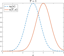
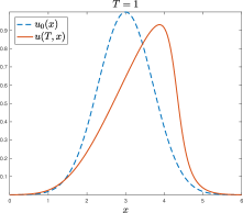
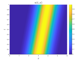
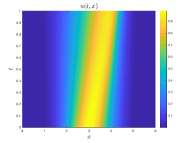
Figure 2: BDF integration of the system of ODEs (21) used as BGK approximation to the conservation law (11). Two velocities are considered, $N=2$. Left-hand side column corresponds to pure transport situation $F(u)=u$, whether the right-hand side column depict the solution of the Burger flux function, $F(u)=u^{2}/2$. Top row show initial data $u_{0}(x)$ as well as the numerical result at terminal time $T=1$, bottom row shows the density $u(x,t)$ in the space-time frame $[0,6]\times[0,1]$. Each test has been produced using a BDF(3) scheme with $N_{x}=640$ space points and $\Delta t=4.47127\times 10^{-3}$, and with fixed relaxation parameter $\epsilon=0.01$.

We do not present convergence tables for the forward equation since equation (21) requires to evaluate the local equilibrium at gridpoints $x+v_{j}t$ that are in general not aligned with the numerical grid. Therefore, an interpolation is required. Hence, the temporal and spatial resolution are not independent and the observed convergence is limited to the interpolation of the solution.

Adjoint system.

A similar behavior is observed for the discretization of the adjoint equation (23). In order to illustrate the results we only show the BDF(2) method applied to (26) in the case of $F(u)=u.$ We use the same parameters as above for the forward system, but now the data $u_{0}(x)$ is prescribed at terminal time $T=1$, in the following way $\lambda^{j}(T,x)=u_{0}(x)/N$, with $N=2$. Then, the adjoint variables are evolved according to the derived scheme (26). For illustration purposes the solutions $p(t,x)=\lambda^{1}(t,x)+\lambda^{2}(t,x)$ are reported for different values of the scaling term $\epsilon$ in Figure 3, in the top row we represent the adjoint equation at time zero jointly with the terminal conditions $p_{T}(x)$, in the bottom row the density $p(t,x)$ in the domain $[0,6]\times[1,0]$. Compared with the Figure 3 we observe that the profile moves over time in the opposite direction, when $\epsilon$ is small enough. This is precisely as expected by the limiting equation $-p_{t}-F^{\prime}(u)p_{x}=0$, where $p=\sum_{j}\lambda^{j}.$

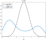
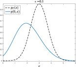
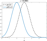
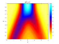
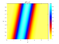
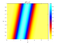
Figure 3: The BDF(2) integration of the system of (26) has been implemented for the linear transport $F(u)=u.$ Two velocities are considered, with $N_{x}=640$ space points and $\Delta t=4.47127\times 10^{-3}$. From left to right we show different values of $\epsilon$, with $\epsilon\in{\{1,0.1,0.0001\}}$. In the top row the terminal data $p_{T}(x)$, $T=1$, as well as the numerical result at initial time $p(0,x)$ are reported for the different values of $\epsilon$. Bottom row depict the density $p(t,x)=\lambda^{1}(t,x)+\lambda^{2}(t,x)$ for the different value of $\epsilon$. Note that for small $\epsilon$ the pure transport equation is obtained.

Finally, we study the dependence of the adjoint equation on the parameter $\epsilon.$ Note that for equation (21) a similar study has been performed in [18]. For each fixed value of $\epsilon$ we compute the average converge rate on the numerical grid given above. We also record the minimal error as well as the minimal used time step. The study is done for the BDF(2) scheme and the results are reported in Table 4.

Table 4: BDF integration of the system of ODEs (23). Two velocities are considered and the $L^{2}$ error of $p=\lambda^{1}+\lambda^{2}$ at initial time is reported. Various values of $\epsilon$ are considered. The mean convergence rate on given grid is reported as well as the finest temporal grid size considered.

$\epsilon$	$\Delta t=\Delta x$	$L^{2}p$	Rate
1	0.00447127	8.75403e-06	2.74404
1.000000e-01	0.00447127	6.63095e-06	2.68572
1.000000e-02	0.00447127	1.77628e-05	2.62852
1.000000e-03	0.00447127	2.08908e-05	2.6135
1.000000e-04	0.00447127	2.12566e-05	2.61174

4.5 Optimal control of hyperbolic balance laws

We finally show the quality of our approach by two applications to the optimal control of hyperbolic balance laws. For further references, and example about optimal control problems governed by conservation laws we refer to [9, 22].

4.5.1 Jin-Xin relaxation system

We consider the Jin-Xin relaxation model, [26] which results in the two velocities model (13), as follows

$$\begin{split}f^{(1)}_{t}+af^{(1)}_{x}&=\frac{1}{\epsilon}\left(E_{1}(u)-f^{(1)}\right),\qquad f^{(1)}(x,0)=f^{(1)}(x)\\ f^{(2)}_{t}-af^{(2)}_{x}&=\frac{1}{\epsilon}\left(E_{2}(u)-f^{(2)}\right),\qquad f^{(2)}(x,0)=f^{(2)}(x)\end{split}$$ (31)

where the equilibrium states $E_{1}$ and $E_{2}$ are given by

$$E_{1}(u)=\frac{1}{2a}\left(au+F(u)\right),\quad E_{2}(u)=\frac{1}{2a}\left(au-F(u)\right),$$

with total density $u=f^{(1)}+f^{(2)}$ and velocity in the limit $\epsilon\to 0$ such that $v=a(f^{(1)}-f^{(2)})=F(u)$. In particular we choose as an example the flux $F(u)=u^{2}/2$ associated to the inviscid Burger equation. Thus we have that the characteristic speed $a$ has to satisfy the condition $a\geq\max_{x\in\mathbb{R}}|u_{0}(x)|.$ We consider the following optimal control problem, firstly proposed in [22], where here we seek for minimizers $f^{(j)}_{0}(x)$, with $j=1,2$ of

$$J(u(\cdot,T),u_{d}(\cdot))=\frac{1}{2}\int_{\Omega}|u(x,T)-u_{d}(x)|^{2}\,dx$$ (32)

Hence we fix the specific domain $\Omega=[-3,3]$ with $T=3$ and we want to prescribe the final discontinuous data $u_{d}(x)$, as final data at time $T$ of the Burger equation with initial data defined as follows

$$u_{d}(0,x)=\begin{cases}1.5+x\qquad\textrm{if}\quad-1.5\leq x\leq-0.5,\\ 0\qquad\textrm{otherwise.}\end{cases}$$ (33)

In order to solve numerically this optimal control problem we approximate it with the optimal control (22)–(20), choosing $N=2$ velocities and $N_{x}=120$ space points, time step $\Delta t=0.05$ and relaxation parameter $\epsilon=10^{-2}$. In order to solve the time discretization we use BDF(2) integration. The same choice of parameters is considered for the adjoint equation (23), which is solved backward in time using a two velocities approximation of the terminal condition $\lambda^{(1)}(T,x)+\lambda^{(2)}(T,x)=p(T,x)=u(x,T)-u_{d}(x)$. Thus, we solve recursively the forward approximated system (20) and the backward system (23), using as starting point the step function $u^{(0)}_{0}(x)=0.5\chi_{[-1.5,-0.5]}(x)$, and introducing a filter $\mathcal{F}(\cdot)$ to reduce the total variation of the initial data $u^{(k)}_{0}$ following the approach in [22]. Then we update the initial data $u_{0}^{(0)}(x)$ using a steepest descend method as follows

$$u^{(k+1)}_{0}=u_{0}^{(k)}-\sigma_{k}p^{(k)},\qquad m\geq 0,$$

with $\sigma_{k}$ updated with Barzilai-Browein step method [3].

We report in Figure 4 the final result after $k=30$ iterations of the optimization process, on the left-hand side plot we depict the initial data $u^{(100)}_{0}$ with the terminal data $u(T,x)$ as well as the desired data $u_{d}(x)$. On the right hand side we depict the decrease of $J(u^{(k)})$given by the optimization procedure.

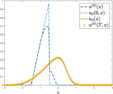
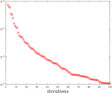
Figure 4: Jin-Xin relaxation system. On the left-hand side we report the control at iteration 100, $u^{(100)}_{0}$ (--), compared with the initial data $u_{d}(0,x)$ (-.) used to compute the desired final data $u_{d}(x)$ (-). The terminal solution $u(T,x)$, (o), is reported and it is computed solving system (31) using BDF(2) integration, with $N_{x}=120$ space points, time step $\Delta t=0.05$, and relaxation parameter $\epsilon=10^{-2}$. On the right-hand side we show the decrease of the functional $J(u^{(k)})$.

4.5.2 Broadwell model

We consider the one-dimensional Broadwell model, [6], which describe the evolution of densities $f^{(1)},f^{(2)},f^{(3)}$ relative to the velocities $c,-c,0$, with $c>0$, as follows

$$\begin{aligned} &f^{(1)}_{t}+cf^{(1)}_{x}=\frac{1}{\epsilon}\left(E_{1}(\rho,m)-f^{(1)}\right),\qquad f^{(1)}(x,0)=f^{(1)}_{0}(x),\\ &f^{(2)}_{t}-cf^{(2)}_{x}=\frac{1}{\epsilon}\left(E_{2}(\rho,m)-f^{(2)}\right),\qquad f^{(2)}(x,0)=f^{(2)}_{0}(x),\\ &f^{(3)}_{t}=\frac{1}{\epsilon}\left(E_{3}(\rho,m)-f^{(3)}\right),\quad\qquad\qquad f^{(3)}(x,0)=f^{(3)}_{0}(x).\end{aligned}$$ (34)

Where the equilibrium quantities are defined as follows

$$E_{1}(\rho,m,z) =\frac{1}{2}F(\rho,m)+\frac{m}{2c},$$

$$E_{2}(\rho,m,z) =\frac{1}{2}F(\rho,m)-\frac{m}{2c},$$

$$E_{3}(\rho,m,z) =-F(\rho,m)+\rho$$

and the macroscopic quantities $m,\rho$, jointly with the flux $F(\rho,m)$ are such that

$$\rho=f^{(1)}+f^{(2)}+2f^{(3)},\qquad m=c(f^{(1)}-f^{(2)}),\qquad F(\rho,m)=\frac{m^{2}}{c^{2}\rho}+\rho.$$ (35)

Indeed for $\epsilon\to 0$ system (LABEL:eq:relaxIE) converges to to the isentropic Euler model, [22], where $\rho,m$ represent respectively density, and momentum,

$$\begin{cases}\rho_{t}+m_{x}=0,\\ m_{t}+c^{2}\left(\frac{m^{2}}{c^{2}\rho}+\rho\right)_{x}=0,\qquad(x,t)\in\mathbb{R}\times(0,T]\end{cases}$$ (36)

We aim to minimize the functional

$$J(\rho(\cdot,T),m(\cdot,T))=\frac{1}{2}\int_{\Omega}\left(|\rho(x,T)-\rho_{d}(x)|^{2}+|m(x,T)-m_{d}(x)|^{2}\right)\ dx$$ (37)

with respect to the initial data $f^{j}_{0}(x)$ for $j=1,2,3$ taking in to account the relations (35). To this end we compute the adjoint equation system associated to (LABEL:eq:relaxIE), and equivalently to (23) we obtain the following

$$- \lambda^{(1)}_{t}-c\lambda^{(1)}_{x}=-\frac{1}{\epsilon}\left(\lambda^{(1)}-\sum_{k}\lambda^{(k)}\left(\partial_{\rho}E_{k}(\rho,m)+c\partial_{m}E_{k}(\rho,m)\right)\right),$$ (38)

$$- \lambda^{(2)}_{t}+c\lambda^{(2)}_{x}=-\frac{1}{\epsilon}\left(\lambda^{(2)}-\sum_{k}\lambda^{(k)}\left(\partial_{\rho}E_{k}(\rho,m)-c\partial_{m}E_{k}(\rho,m)\right)\right),$$

$$- \lambda^{(3)}_{t}=-\frac{1}{\epsilon}\left(\lambda^{(3)}-\sum_{k}\lambda^{(k)}\partial_{\rho}E_{k}(\rho,m)\right),$$

complemented by the terminal conditions

$$\lambda^{(1)}(T,x)=\partial_{\rho}J(\rho,m)+c\partial_{m}J(\rho,m),\,\lambda^{(2)}(T,x)=\partial_{\rho}J(\rho,m)-c\partial_{m}J(\rho,m),\,\lambda^{(3)}(T,x)=\partial_{\rho}J(\rho,m).$$

We set up the control problem (36)–(37) defining as reference density, and momentum the final state of system (36) at time $T_{f}=0.15$ provided the following initial data

$$\rho_{d}(0,x)=1,\quad x\in[-2.5,2.5],\quad m_{d}(0,x)=\begin{cases}\sin(\pi x),\quad x\in[-1,1]\\ 0\qquad\qquad\textrm{otherwise}.\end{cases}$$ (39)

and zero flux boundary conditions.

In order to solve numerically problem (LABEL:eq:relaxIE) –(38), we fix the relaxation parameter $\epsilon=0.01$. We discretize the space domain with an uniform grid of $N_{x}=320$ points, and with time step $\Delta t=0.01$. In order to reduce the total variation of the initial data $(\rho^{(k)}_{0},m^{(k)}_{0})$ we introduce a filter $\mathcal{F}(\cdot)$ following the strategy proposed in [22]. The optimization step is initialized using as starting guess the following data

$$\rho^{(0)}(0,x)=1,\qquad m^{(0)}(0,x)=0,\quad x\in[-2.5,2.5].$$ (40)

Then at each iteration $k=0,1,\ldots$ the initial data $\rho_{0}^{(k)}(x),m_{0}^{(k)}(x)$ is updated with gradient method with Barzilai-Borwein descent step, [3].

We report in Figure 5 the result of the optimization process. Top row depicts the evolution of the density, whereas bottom row refers to momentum evolution. On the left-hand side the initial value $(\rho^{(0)}_{0}(x),m_{0}^{(0)}(x))$ is compared with the control $(\rho_{0}^{(k)}(x),m_{0}^{(k)}(x))$ obtained after $k=70$ iterations of the optimization process, and the true initial data defined by (LABEL:realID). The right-hand side column depicts the density and momentum at final time $T=0.15$ comparing the reference solution $(\rho_{d}(x),m_{d}(x))$ with respect to $(\rho^{(k)}(T,x),m^{(k)}(T,x))$. Finally Figure 6 reports the decrease of the functional $J(\rho,m)$ evaluated at each iteration of the optimization process.

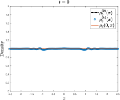
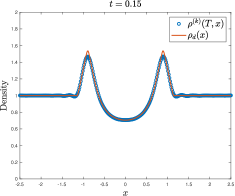
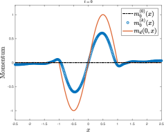
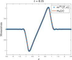
Figure 5: Broadwell model. We consider $\epsilon=0.01$, using $N_{x}=320$ space points and $\Delta t=1\times 10^{-2}$. Top row represents the initial and final time of the density $\rho(t,x)$, comparing the optimal control $\rho^{(k)}$ with respect to the reference $\rho_{d}$ at initial (left plot) and final time (right plot). Bottom row compares the momentum $m^{(k)}(t,x)$ at initial (left plot) and final time (right plot) with respect to the reference solution $m_{d}(x)$.

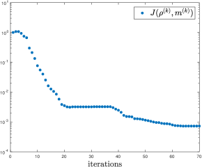
Figure 6: Broadwell model. Decrease of the functional $J(\rho,m)$ evaluated in $\rho^{(k)},m^{(k)}$, at each iteration $k$ of the optimization process.

5 Conclusion

We analyze linear multi-step schemes for control problems of ordinary differential equations and hyperbolic balance laws. In the case of ordinary differential equations we show theoretically and numerically that only BDF methods are consistent discretization of the corresponding optimality systems up to high–order. The BDF methods may also be used as higher order discretization of relaxation systems in combination with a Lagrangian scheme. We derive the corresponding adjoint equations and we show that this system can again be discretized by a BDF type method. The numerically observed convergence rates confirm the expected behavior both for ordinary differential systems, as well as hyperbolic balance laws.

Appendix A Definition of BDF, Adams–Moulton and Adams–Bashfort Formulas

In view of the scheme (4) each scheme is represented by two vectors $a,b$ with $a=(a_{0},\dots,a_{s-1})\in\mathbb{R}^{s}$ and $b=(b_{-1},b_{0},\dots,b_{s-1})\in\mathbb{R}^{s+1}$ for an $s-$stage scheme. Only in the case of BDF schemes we have $b\in\mathbb{R}^{s+1},$ otherwise we have $b\in\mathbb{R}^{s}.$ For the schemes implemented in this paper we use the following schemes.

Name	s	$a^{t}$	$b^{t}$
Implicit Euler (BDF(1))	1	-1	(1,0)
Explicit Euler	1	0	(0,1)
BDF methods
BDF(2)	2	(-4/3,1/3)	(2/3,0,0)
BDF(3)	3	(-18/11,9/11,-2/11)	(6/11,0,0,0)
BDF(4)	4	(-48/25,36/25,-16/25,3/25)	( 12/25,0,0,0,0)
Adams–Bashfort (AB) methods
AB(2)	2	(-1,0)	(0,3/2,-1/2)
AB(3)	3	(-1,0,0)	(0,23/12,-4/3,5/12)
Adams–Moulton (AM) methods
AM(4)	4	(-1,0,0,0)	(251,646,-264,106,-19)/270

Acknowledgments

This work has been supported by DFG HE5386/13,14,15-1, by the DAAD–MIUR project, KI-Net and by the INdAM-GNCS 2018 project Numerical methods for multi-scale control problems and applications.

References

• [1] G. Albi, M. Herty, C. Jörres and L. Pareschi, Asymptotic preserving time-discretization of optimal control problems for the Goldstein-Taylor model, Numer. Meth. Partial Diff. Equations, 30 (2014), 1770–1784.
• [2] M. K. Banda and M. Herty, Adjoint IMEX–based schemes for control problems governed by hyperbolic conservation laws, Comp. Opt. and App., (2010), 1–22.
• [3] J. Barzilai, J. M. Borwein. Two-point step size gradient methods. IMA journal of numerical analysis, 8(1), (1988) 141–148.
• [4] J. F. Bonnans and J. Laurent-Varin, Computation of order conditions for symplectic partitioned Runge-Kutta schemes with application to optimal control, Numerische Mathematik, 103 (2006), 1–10.
• [5] P.L. Bhatnagar, E.P. Gross and K. Krook, A model for collision processes in gases, Phys. Rev. 94 (1954) 511-525.
• [6] J. Broadwell, Shock structure in a simple discrete velocity gas. The Physics of Fluids, 7(8), (1964) 1243-1247.
• [7] R. Caflisch, J. Shi, G. Russo, Uniformly accurate schemes for hyperbolic systems with relaxation. SIAM Journal on Numerical Analysis 34.1 (1997) 246-281.
• [8] E. Carlini, A. Festa, F. Silva, M.T. Wolfram. A semi-Lagrangian scheme for a modified version of the Hughes’ model for pedestrian flow. Dynamic Games and Applications, 7(4), (2017) 683–705.
• [9] A. Chertock, M. Herty, A. Kurganov. An Eulerian–Lagrangian method for optimization problems governed by multidimensional nonlinear hyperbolic PDEs. Computational Optimization and Applications, 59(3), (2014) 689–724.
• [10] M. Chyba, E. Hairer and G. Vilmart, The role of Symplectic integrators in optimal control, Opt. Control App. and Meth., (2008)
• [11] G. Dimarco and R. Loubere, Towards an ultra efficient kinetic scheme. Part I: Basics on the BGK equation, J. Comput. Phys. 255 (2013) 680-698.
• [12] G. Dimarco and L. Pareschi, Numerical methods for kinetic equations, Acta Numerica, 23, (2014), 369–520.
• [13] G. Dimarco and L. Pareschi, Implicit-explicit linear multistep methods for stiff kinetic equations, SIAM J. Numer. Anal. 55 (2017), no. 2, 664–690
• [14] A. L. Dontchev and W. W. Hager, The Euler approximation in state constrained optimal control, Math. Comp., 70 (2001), 173–203
• [15] A. L. Dontchev, W. W. Hager and V. M. Veliov, Second–order Runge–Kutta approximations in control constrained optimal control, SIAM J. Numer. Anal., 38 (2000), 202–226
• [16] M. Falcone, R. Ferretti, Convergence analysis for a class of high-order semi-Lagrangian advection schemes. SIAM Journal on Numerical Analysis, 35(3), (1998) 909-940.
• [17] F. Filbet and G. Russo, Semilagrangian schemes applied to moving boundary problems for the BGK model of rarefied gas dynamics, Kinet. Relat. Models 2 (2009) 231-250.
• [18] M. Groppi, G. Russo and G. Stracquadanio, High order semilagrangian methods for the BGK equation, Comm. Math. Sci., 14(2), (2016), 389–414
• [19] W. W. Hager, Runge-Kutta methods in optimal control and the transformed adjoint system, Numerische Mathematik, 87 (2000), 247–282.
• [20] E. Hairer, C. Lubich and G. Wanner, Geometric Numerical Integration. Structure-Preserving Algorithms for Ordinary Differential Equations, Springer Series in Computational Mathematics, 2nd edition (2006).
• [21] E. Hairer, S. P. Nørsett and G. Wanner, Solving Ordinary Differential Equations, Part I. Nonstiff Problems, Springer Series in Computational Mathematics, 2nd edition (1993).
• [22] M. Herty, A. Kurganov and D.  Kurochkin, Numerical method for optimal control problems governed by nonlinear hyperbolic systems of PDEs, J. Commun. Math. Sci.13(1) (2015), 15–48.
• [23] M. Herty, L. Pareschi and S. Steffensen Implicit–Explicit Runge-Kutta schemes for numerical discretization of optimal control problem, SIAM J. Num. Analysis 51(4) (2013).
• [24] M. Herty and V. Schleper, Time discretizations for numerical optimization of hyperbolic problems, App. Math. Comp. 218 (2011), 183–194.
• [25] M. R. Hestenes, Calculus of Variations and Optimal Control Theory, Wiley&Sons, Inc., New York (1980).
• [26] S. Jin and Z. Xin, The relaxation schemes for systems of conservation laws in arbitrary space dimension, Comm. Pure and Appl. Math. 48, (1995), 235–276.
• [27] C.Y. Kaya, Inexact Restoration for Runge-Kutta Discretization of Optimal Control Problems, SIAM J. Numer. Anal., 48 (2010), 1492–1517.
• [28] J. Lang and J. Verwer W-Methods in optimal control Numer. Math., 124(2), (2013), 337–360
• [29] J.M.T. NgnotchouyeI, M. Herty, S. Steffensen and M.K. Banda, Relaxation approaches to the optimal control of the Euler equations, Comput. Appl. Math., Vol. (30)(2) (2011).
• [30] L. Pareschi, Characteristic-based relaxation methods for hyperbolic conservation laws with stiff nonlinear terms, Rendiconti Circolo Matematico di Palermo, Serie II, 57 (1998), pp.375–380.
• [31] L. Pareschi, Central differencing based numerical schemes for hyperbolic conservation laws with relaxation terms. SIAM Journal on Numerical Analysis 39.4 (2001): 1395-1417
• [32] G. Russo, P. Santagati and S.-B. Yun Convergence of a semi-lagrangian scheme for the BGK model of the Boltzmann equation, SIAM J. on Numer. Anal. 50 (2012) 1111-1135.
• [33] A. Sandu, On Consistency Properties of Discrete Adjoint Linear Multistep Methods, Computer Science Technical Report TR-07-40, 2007
• [34] A. Sandu, On the properties of Runge–Kutta discrete adjoints, Lecture Notes in Computer Science 3394 (2006) 550–557
• [35] D. Schröder, J. Lang and R. Weiner Stability and consistency of discrete adjoint implicit peer methods, J. Comput. Appl. Math. 262 (2014) 73–86.
• [36] J. L. Troutman, Variational Calculus and Optimal Control, Springer, New York (1996)
• [37] A. Walther, Automatic differentiation of explicit Runge–Kutta methods for optimal control, J. Comp. Opt. Appl., 36 (2007), 83–108.