Radio pulsars: already fifty years!
100 years of Uspekhi Fizicheskich Nauk Journal

Abstract

Although fifty years have passed since the discovery of radio pulsars, there is still no satisfactory understanding of how these amazing objects operate. While there has been significant progress in understanding the basic properties of radio pulsars, there is as yet no consensus on key issues, such as the nature of coherent radio emission or the conversion mechanism of the electromagnetic energy of the pulsar wind into particle energy. In this review, we present the main theoretical results on the magnetosphere of neutron stars. We formulate a number of apparently simple questions, which nevertheless remain unanswered since the very beginning of the field and which must be resolved before any further progress can be made.

1 Pulsar chronicles

1.1 Prehistoric period (before 1967)

The possible existence of neutron stars (with a mass of the order of the solar mass, $M\approx M_{\odot}=1.99\times 10^{33}$ g, having a radius $R$ of only 10–15 km) was known long before the discovery of radio pulsars. They were predicted by Baade and Zwicky [1] as early as the mid-1930. However, due to their very small diameter, it had been thought for a long time that it would be very difficult to detect single neutron stars. Just several months before the discovery of pulsars did Pacini [4] surmised that such stars should have very short rotational periods, $P\sim 1$ s, and superstrong magnetic fields, $B_{0}\sim 10^{12}$ G, and therefore should be powerful energy sources; however, it was not stated in [4, 5], of course, that neutron stars should be bright cosmic radio sources. For this reason, no dedicated searches for these objects were organized and pulsars were serendipitously detected in 1967 by Bell and Hewish during a different observational program [6]. We recall that the possibility of detecting thermal X-ray emission from accreting neutron stars in close binary systems was clearly formulated in [7-9], and X-ray pulsars were indeed discovered soon after the launch of the first X-ray telescope [10].

1.2 Hellas (1968–1973)

The period 1968-1973 is a remarkable era of simple and visual ideas, which nevertheless enabled intuitive understanding of the nature of physical processes in pulsars. Indeed, what can be apparently simpler than a magnetized ball rotating in a vacuum? Such a simple model turned out to be sufficient for describing the main properties of radio pulsars [11]. For example, it soon became quite clear that the rotation of a neutron star underlies the extremely stable pulse arrival time [12, 13] and the kinetic energy of rotation is the energy reservoir for the activity of radio pulsars.

Simultaneously, as mentioned above, the main idea was formulated according to which the energy release mechanism should be related to electrodynamic processes [4]. To date, the canonical expression for magnetic dipole energy losses,

$$W_{\rm tot}^{({\rm V})}=-I_{\rm r}\Omega\dot{\Omega}=\frac{1}{6}\,\frac{B_{0}^{2}\Omega^{4}R^{6}}{c^{3}}\sin^{2}\chi\approx 10^{32}\frac{B_{12}^{2}}{P^{4}}\,\,{\rm erg}\,{\rm s^{-1}}$$ (1)

(where $B_{0}$ is the polar magnetic field, $I_{\rm r}\sim MR^{2}$ is the moment of inertia, and $\chi$ is the magnetic dipole inclination angle with the spin axis), has been used to estimate radio pulsar energy losses. Here and below in similar formulas, we use the notation $B_{12}=B_{0}/(10^{12}$ G) and ${\dot{P}}_{-15}={\dot{P}}/10^{-15}$, and express the period $P=2\pi/\Omega$ in seconds. By inverting equation (1), we obtain a very simple expression for the magnetic field estimate

$$B_{12}\approx(P{\dot{P}}_{-15})^{1/2}.$$ (2)

We recall that the eureka moment was related exactly to expression (1), because after the discovery of a pulsar in the Crab Nebula ($P\approx 33$ ms, ${\dot{P}}_{-15}\approx 420$) two values already known by that time — the total power of the Crab nebula $L_{\rm tot}\approx 5\times 10^{38}$ erg s^-1 (this energy should be permanently injected into the nebula to provide its optical emission due to synchrotron losses) and the so-called dynamical age $\tau_{\rm D}=P/2{\dot{P}}\approx 1000$ years corresponding to the historical supernova 1054AD — were naturally explained.

By the way, this simple model enabled the first step towards understanding that radio pulsars can be sources of cosmic rays; for millisecond pulsars (the fastest pulsar among the more than 2600 known to date indeed has the period $P\approx 1.39$ ms) and sufficiently high magnetic fields $B_{0}\sim 10^{13}$ G, the potential difference between the pole and the equator of a rotating magnetized sphere,

$$\Delta V\approx\left(\frac{\Omega R}{c}\right)B_{0}R,$$ (3)

reaches $10^{20}$ eV, i.e., corresponds to the maximum energy observed in cosmic rays. A similar estimate was also made by Ostriker and Gunn [14] for the energy of particles accelerated in an electromagnetic wave propagating from a rotating neutron star. If all radio pulsars were born with sufficiently shot periods (now it is fully clear that this is not the case [15]), the problem of the origin of cosmic rays could be solved [16,17].

However, in a few years, it had already become clear that a magnetized sphere rotating in a vacuum is too far away from reality. In 1971 Sturrock showed in [18] that in the super strong magnetic field of a pulsars, the process of single-photon conversion of hard gamma-ray photons into electron-positron pairs should play a crucial role

$$\gamma+(B)\rightarrow e^{+}+e^{-}+(B).$$ (4)

As a result, the neutron star magnetosphere is very quickly filled up with charged particles, which must inevitably result in the total restructuring of the braking mechanism of radio pulsars.

Indeed, the rotation of a magnetized neutron star in a vacuum inevitably leads to the appearance of a longitudinal (parallel to magnetic field) electric field $E_{\parallel}\sim(\Omega R/c)B$ outside the neutron star. Any primary charged particle entering this region would be accelerated up to ultrarelativistic energies, ${\cal E}_{\rm e}\gg m_{\rm e}c^{2}$. Due to the extremely short time of synchrotron losses, which in magnetic fields $B_{0}\sim 10^{12}$ G for electrons (and positrons) is only

$$\tau_{\rm s}\sim\frac{1}{\omega_{B}}\left(\frac{c}{\omega_{B}r_{\rm e}}\right)\sim 10^{-15}\,{\rm c},$$ (5)

(here and below $\omega_{B}=eB/m_{\rm e}c$ is the gyrofrequency and $r_{\rm e}=e^{2}/m_{\rm e}c^{2}$ is the classical radius of an electron), the particles can move along magnetic field lines only. But because the magnetic field lines are curved, the primary particles must emit hard gamma-ray quanta with the characteristic energy (so-called ‘curvature radiation’ [19])

$${\cal E}_{\rm ph}=\hbar\omega_{\rm cur}\sim\frac{\hbar c}{R_{\rm c}}\,\left(\frac{{\cal E}_{\rm e}}{m_{\rm e}c^{2}}\right)^{3},$$ (6)

where $R_{\rm c}$ is the curvature radius of a magnetic field line. Just the curvature radiation losses impose a bound on the particle energy ${\cal E}_{\rm e}$. Indeed, writing the energy equation in the form

$$\frac{{\rm d}{\cal E}_{\rm e}}{{\rm d}l}=eE_{\parallel}-\frac{2}{3}\,\frac{e^{2}}{R_{\rm c}^{2}}\left(\frac{\cal E_{\rm e}}{m_{\rm e}c^{2}}\right)^{4},$$ (7)

we obtain the maximum energy of the primary particles

$${\cal E}_{\rm max}\sim\left(\frac{R_{\rm c}^{2}E_{\parallel}}{e}\right)^{1/4}m_{\rm e}c^{2}\sim(10^{7}-10^{8})\,{\rm MeV}.$$ (8)

Next, by propagating almost rectilinearly in the curved magnetic field, the curvature radiation quanta start moving at increasingly large angles $\theta_{\rm b}$ to the magnetic field, to ultimately produce secondary electron-positron pairs (the synchrotron photons generated by the secondary particles from their transitions to the ground Landau levels also play a role here). This is because for a photon with an energy ${\cal E}_{\rm ph}$ propagating at an angle $\theta_{\rm b}$ to the magnetic field ${\bf B}$, far from the threshold ${\cal E}_{\rm ph}=2m_{\rm e}c^{2}$ the probability of single-photon conversion (4) has the form [20]

$$w=\frac{3\sqrt{3}}{16\sqrt{2}}\,\frac{e^{3}B\sin\theta_{\rm b}}{\hbar m_{\rm e}c^{3}}\exp\left(-\frac{8}{3}\frac{B_{\rm cr}}{B\sin\theta_{\rm b}}\frac{m_{\rm e}c^{2}}{{\cal E}_{\rm ph}}\right),$$ (9)

where

$$B_{\rm cr}=\frac{m_{\rm e}^{2}c^{3}}{e\hbar}\approx 4.4\times 10^{13}\,{\rm G}$$ (10)

is the critical magnetic field at which the energy gap between two adjacent Landau levels is of the order of the rest-mass energy of the electron: $\hbar\omega_{B}=m_{\rm e}c^{2}$. Hence, for not too long mean free paths of photons, $l_{\gamma}<R$, we obtain the simple estimate

$$l_{\gamma}=\frac{8}{3\Lambda}R_{\rm c}\frac{B_{\rm cr}}{B}\,\frac{m_{\rm e}c^{2}}{{\cal E}_{\rm ph}},$$ (11)

where the logarithmic factor for the characteristic parameters near the neutron star surface is

$$\Lambda\approx\ln\left[\frac{e^{2}}{\hbar c}\,\frac{\omega_{B}R_{\rm c}}{c}\left(\frac{B_{\rm cr}}{B}\right)^{2}\left(\frac{m_{\rm e}c^{2}}{{\cal E}_{\rm ph}}\right)^{2}\right]\sim 20.$$ (12)

We recall that unlike an electric field, the magnetic field cannot create particles. However, it can play the role of a catalyst, enabling the energy and momentum conservation for the process being considered. This is why the creation of a pair is prohibited for a photon propagating along the magnetic field lines: the probability of pair creation (9) is zero in this case.

As a result, the process of secondary particle creation precipitously increases due to the acceleration of secondary particles and their emission of curvature photons, etc. This process stops only when the secondary electron-positron plasma screens the longitudinal electric field $E_{\parallel}$. Incidentally, this means that radio pulsars should also be sources of positrons, albeit much less energetic than follows from estimate (3).

Thus, it became clear that pulsar magnetospheres should be filled with electron-positron plasma. Therefore, since the 1970s, a more realistic magnetosphere model has been considered, in which the longitudinal electric field is fully screened ($E_{\parallel}=0$). Indeed, the appearance of a longitudinal electric field in some region would immediately lead to abrupt plasma acceleration and hence to an explosive creation of secondary particles.

On the other hand, it is well known that in a fully screened longitudinal electric field, the plasma starts rigidly rotating together with the star, as in Earth’s and Jupiter’s magnetospheres [21]. It is this plasma property that proved to be crucial to understanding the pulsar activity.

First of all, the rigid rotation becomes impossible at sufficiently large distances from the rotation axis, $r_{\perp}>R_{\rm L}$, where the rotation velocity exceeds the speed of light (Fig. 1). Here,

$$R_{\rm L}=\frac{c}{\Omega}$$ (13)

is the so-called light cylinder radius. For ordinary radio pulsars with periods of $0.1$–$1$ s, we have $R_{\rm L}\sim$ $10^{9}$–$10^{10}$ cm, which means that the light cylinder lies at a distance of thousand times the neutron star radius. Next, it is easy to estimate the size of the polar cap, $R_{\rm cap}\approx R_{0}$, where

$$R_{0}=\left(\frac{\Omega R}{c}\right)^{1/2}R,$$ (14)

which is the region around the magnetic poles of a neutron star from which the magnetic field lines go beyond the light cylinder. For ordinary radio pulsars, the polar cap size is just several hundred meters. Hence, the polar cap area can be conveniently written as $s=f_{\ast}\pi R_{0}^{2}$, where $f_{\ast}\approx 1$.

The importance of polar caps stems from the fact that charged particles moving along magnetic field lines can escape the neutron star magnetosphere. As noted above, such a motion arises not only due to small Larmor radii compared to other characteristic scales but also because of an extremely short synchrotron cooling time. As a result, two sets of magnetic field lines appear. The open field lines coming out of the polar caps cross the light cylinder and go from the magnetosphere to infinity, whereas other field lines close inside the light cylinder. The plasma within the closed region turns out to be trapped, while the particles moving along the open field lines can leave the magnetosphere.

That simple magnetospheric model allowed Radhakrishnan and Cooke [22] (and later Oster and Sieber [23]) to formulate the so-called ‘hollow cone model’, which remarkably explained all basic morphological properties of pulsar radio emission. Indeed, secondary plasma generation should be suppressed near the magnetic poles, where, thanks to almost rectilinear magnetic field lines, the curvature radiation intensity is also significantly reduced and, in addition, the curvature gamma quanta emitted by relativistic particles propagate at small angles to the magnetic field, which also reduces the secondary pair creation probability.

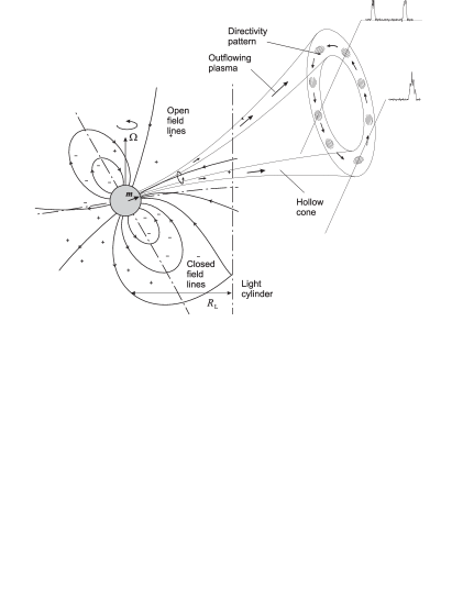
Figure 1: Basic elements of the pulsar magnetosphere and the geometric ‘hollow cone’ model. The potential drop near the magnetic poles results in additional rotation of the outflowing plasma around the magnetic axis. Here and below, pluses and minuses indicate the sign of the charge density.

As a result, as shown in Fig. 1, it is possible to assume that in the central part of the open field lines, the density of the outflowing plasma is strongly reduced. Now, assuming quite reasonably that the radio emission is directly related to the outflowing relativistic plasma, a significant decrease in the radio emission can be expected in the central part of the radio beam. As a result, for the lateral crossing of the directivity pattern, we should expect to observe a single mean pulse profile, while for the central crossing, a two-hump profile should be observed. Without going into the details, we note that just such a situation occurs in reality [24].

In these first years of radio pulsar studies, three main parameters determining the key electrodynamic processes were defined. The first was the electric charge density that is needed to screen the longitudinal electric field near the neutron star surface,

$$\rho_{\rm GJ}=-\frac{{\bf\Omega\cdot B}}{2\pi c}.$$ (15)

This quantity, introduced by Goldreich and Julian in 1969 [25], determines the characteristic particle number density $n_{\rm GJ}=|\rho_{\rm GJ}|/|e|$ (of the order of $10^{12}$ cm^-3 near the neutron star surface) and also the characteristic current density, $j_{\rm GJ}=c\rho_{\rm GJ}$, which is much more important. As we see in what follows, it is the longitudinal electric current circulating in the magnetosphere that will play the key role. The second parameter is the particle multiplication factor $\lambda$,

$$\lambda=\frac{n_{\rm e}}{n_{\rm GJ}},$$ (16)

which shows how much the secondary particle number density exceeds the critical number density $n_{\rm GJ}$. Finally, the third parameter is the so-called magnetization parameter $\sigma_{\rm M}$

$$\sigma_{\rm M}=\frac{1}{4\lambda}\,\frac{eB_{0}\Omega^{2}R^{3}}{m_{\rm e}c^{4}},$$ (17)

also introduced in 1969 by Michel [26]. It is equal to a maximum possible Lorentz factor of particles, $\gamma_{\rm max}$, which is achieved if all the energy $W_{\rm tot}$ (1) is converted into the hydrodynamic particle flow ${\dot{N}}m_{\rm e}c^{2}\Gamma$. Here

$${\dot{N}}=\lambda\pi R_{0}^{2}n_{\rm GJ}c$$ (18)

is the electron-positron pair injection rate, and $\Gamma$ here and below denotes the hydrodynamic Lorentz factor of the outflowing plasma. In formula (17), we added the subscript ‘M’ because $\sigma$ is now commonly used for another quantity, $\sigma=\sigma_{\rm M}/\Gamma=W_{\rm em}/W_{\rm part}$, the ratio of the electromagnetic energy flux to the particle energy flux. Using formula (1), we can rewrite definition (17) in the very simple form [27]

$$\sigma_{\rm M}=\frac{1}{\lambda}\left(\frac{W_{\rm tot}}{W_{\rm A}}\right)^{1/2}.$$ (19)

where $W_{\rm A}=m_{\rm e}^{2}c^{5}/e^{2}\approx 10^{17}$ erg s^-1 is the minimum power of the ‘central engine’ enabling particle acceleration to relativistic energies ($\sigma_{\rm M}\sim 1$ for $\lambda=1$ and $W_{\rm tot}=W_{\rm A}$).

Thus, during the first several years after the discovery of radio pulsars, answers to most of the key questions were obtained (the periodicity of pulses is related to rotation, the energy source is the kinetic energy of rotation, the energy release is due to the electrodynamic mechanism). Naturally, it remained to be understood how all this works. It was necessary to understand how the energy is carried away from a rotating neutron star to infinity; what the energy spectrum of the outflowing plasma is; and, of course, what the mechanism of the observed coherent radio emission is (and this mechanism indeed must be coherent, because the brightness temperature is usually $T_{\rm br}\sim 10^{28}$ K [15] and in individual giant pulses can be as high as $10^{38}$ K [28]). To date, the answers to most of these questions are unknown.

1.3 Rome (1973–1983)

In this period, the first rigorous laws were formulated concerning all the main topics of the field, including secondary plasma generation, the pulsar magnetosphere structure, and the pulsar wind problem. First of all, two detailed models of electron-positron pair generation near the neutron star surface were proposed. This process is made possible due to the continuous plasma outflow along open field lines, which results in the formation of a region with a longitudinal electric field (a ‘gap’) above the polar cap. Below, we refer to this region as the inner gap, to distinguish it from other regions in the magnetosphere where longitudinal electric fields can appear. The height of the gap is determined by the secondary particle generation mechanism. At that time, most of the secondary particles were thought to have been created outside the acceleration region of the primary particles, where the longitudinal electric field is already small and the secondary plasma can freely leave the neutron star magnetosphere.

The first model was proposed in 1975 by Ruderman and Sutherland [29], as well as by Eidman’s group [30]. This model assumed that the particle ejection from the star surface is insignificant, because it was thought at that time [31+35] that the work function of particles of the neutron star surface $A_{\rm w}\sim 1$–$5$ keV, which, for example, determines the cold emission current [36, 37]

$$j(E)=\frac{e^{3}\,B_{0}}{8\pi^{2}\hbar c\,(2m_{\rm e}A_{\rm w})^{1/2}}E\,\exp\left[-\frac{(8m_{\rm e}A_{\rm w}^{3})^{1/2}}{3\hbar eE}\right]$$ (20)

is sufficiently high. Accordingly, thermal emission was ignored as well [39] (we discuss it in more detail in Section 2.1.2). As a result, from an analysis of Eqns (6) and (9)-(11), it is easy to obtain an estimate of the potential drop needed for the secondary plasma creation [29]:

$$\psi_{\rm RS} \approx \frac{m_{\rm e}c^{2}}{e}\left(\frac{\hbar}{m_{\rm e}c}\right)^{-3/7}R_{\rm c}^{4/7}R_{\rm L}^{-1/7}\left(\frac{B_{0}}{B_{\rm cr}}\right)^{-1/7}$$ (21)

$$\approx 6\times 10^{12}\,B_{12}^{-1/7}P^{-1/7}R_{7}^{4/7}\,{\rm V}.$$

Here $R_{7}=R_{\rm c}/(10^{7}$ cm). Accordingly, the gap height is

$$H_{\rm RS} \approx \left(\frac{\hbar}{m_{\rm e}c}\right)^{2/7}R_{\rm c}^{2/7}R_{\rm L}^{3/7}\left(\frac{B_{0}}{B_{\rm cr}}\right)^{-4/7}$$ (22)

$$\approx 10^{4}\,B_{12}^{-4/7}P^{3/7}R_{7}^{2/7}\,{\rm cm}.$$

We recall that the condition $\psi_{\rm RS}=\psi_{\rm max}$ (or, equivalently, $H_{\rm RS}=R_{0}$), where

$$\psi_{\rm max}=\frac{1}{2}\,\left(\frac{\Omega R}{c}\right)^{2}RB_{0}$$ (23)

is the maximum possible potential drop in the inner gap region, is the mathematical expression for the ‘death line’ on the $P-{\dot{P}}$ diagram (Fig. 2), below which secondary plasma generation (and hence the activity of a neutron star as a radio pulsar) is impossible. However, later on, when more exact calculations in [40-43] showed that the work function of electrons is a factor of 10 lower than assumed before ($A_{\rm w}\sim 100$ eV), Arons’s group proposed an alternative model in which the potential drop was noticeably smaller,

$$\frac{\psi_{\rm A}}{\psi_{\rm RS}} \approx \left(\frac{\Omega R}{c}\right)^{1/2}.$$ (24)

It is this model with free particle ejection that has been considered as the most appropriate one in the subsequent thirty years, despite the obvious problems that it has (for example, in its original version, particles were generated only in the half of the polar cap closest to the pole).

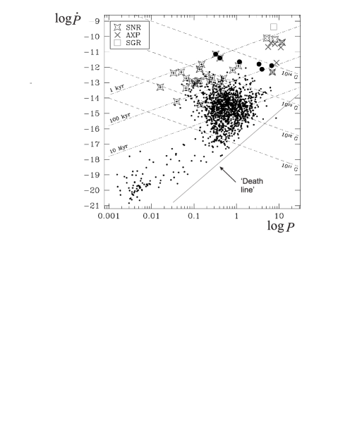
Figure 2: The ‘death line’ on the period $P$—period derivative ${\dot{P}}$ plot corresponding to the Ruderman-Sutherland model [29]. SNR—pulsars in supernova remnants, AXP—anomalous X-ray pulsars, SGR—soft gamma-ray repeaters.

These models have been important because they approximately determined the multiplicity factor of secondary particles l and their energy spectrum. Starting from the first paper by Daugherty and Harding in 1982 [47], it became clear that the plasma multiplicity factor cannot exceed $10^{4}$–$10^{5}$. In particular, this meant that the particle number density near the neutron star surface, $\lambda n_{\rm GJ}\sim 10^{16}$ cm^-3, is too low for the 511 keV annihilation line to be detected. Accordingly, the magnetization parameter $\sigma_{\rm M}$ cannot exceed $10^{3}$–$10^{4}$ for most pulsars and can be as high as $10^{6}$ only for young pulsars (Crab, Vela).

We note that the values of $\lambda$ and $\sigma_{\rm M}$ given above can be easily estimated from the following simple considerations. An analysis of Eqn (7) shows that particles in the inner gap indeed reach energies comparable to the maximum value ${\cal E}_{\rm max}$ in (8). This means that the energy transferred to the curvature radiation photons is also of the order of ${\cal E}_{\rm max}=e\psi_{\rm RS}$. Then the plasma multiplicity $\lambda$ can be estimated as

$$\lambda\sim\frac{{\cal E}_{\rm max}}{{\cal E}_{\rm min}},$$ (25)

where ${\cal E}_{\rm\min}$ is the minimum energy of a photon capable of creating an electron+positron pair. This value can be easily derived from Eqn (11) by setting $l_{\gamma}=R$ because for large photon mean free paths $l_{\gamma}>R$, the neutron star magnetic field starts rapidly decreasing along the gamma-quantum trajectory. As a result, for ordinary pulsars, we obtain

$${\cal E}_{\rm min}\approx\frac{B_{\rm cr}}{\Lambda B}\,\frac{R_{\rm c}}{R}m_{\rm e}c^{2}\sim 10^{2}\,{\rm MeV},$$ (26)

which yields

$$\lambda\sim 10^{5}R_{\rm c,7}^{-3/7}P^{-1/7}B_{12}^{6/7}.$$ (27)

To estimate $\sigma_{\rm M}$, it suffices to use (19), whence we find

$$\sigma_{\rm M}\approx\frac{{\cal E}_{\rm min}}{{\cal E}_{\rm max}}\left(\frac{W_{\rm tot}}{W_{\rm A}}\right)^{1/2}\sim 10^{4}.$$ (28)

We stress that the photon energy ${\cal E}_{\rm\min}$ does not generally coincide with the characteristic maximum energy in the energy spectrum of the secondary particles. This is related to already mentioned synchrotron losses due to which the secondary particles can rapidly lose most of their energy soon after creation. Passing to the reference frame in which the photon propagates perpendicular to the external magnetic field, it is possible to show that after the transition to low-lying Landau levels, the secondary particle energy is

$${\cal E}_{\rm e}\approx\frac{R_{\rm c}}{R}m_{\rm e}c^{2},$$ (29)

(which differs little from (26), however, for magnetic fields $B\sim 10^{12}$ G).

We see that both estimates (26) and (29) demonstrate that the secondary particle energy spectrum essentially depends on the curvature of magnetic field lines. For a dipole magnetic field with the characteristic curvature radius $R_{\rm c}\approx R\,(\Omega R/c)^{-1/2}\sim 10^{7}$–$10^{8}$ cm in the polar cap region , the characteristic particle Lorentz factor is $\gamma_{\rm min}\approx 100$. Exactly these values for the maximum in the energy spectrum of secondary particles were obtained in both the pioneering paper [47] and all subsequent papers [48-51] calculating the outflowing plasma energy spectrum. If, as is frequently assumed recently [52, 53], the near-surface dipole magnetic field is strongly distorted by the multipole components, significantly reducing the curvature radius $R_{\rm c}$ (which is required for the ‘death line’ in the Arons model to be consistent with observations), then the maximum in the secondary particle energy spectrum can decrease to $\gamma_{\rm min}\approx 3$–$10$.

The above formulas can also be used to estimate the electron-positron plasma ejection rate ${\dot{N}}$ and the total number of particles $N=\int{\dot{N}}{\rm d}t$ ejected during the pulsar lifetime:

$${\dot{N}} \approx \lambda\,\frac{B_{0}\Omega^{2}R^{3}}{ce}\sim 3\times 10^{34}\,P^{-2}B_{12}\,{\rm s}^{-1},$$ (30)

$$N \approx \lambda\,\frac{Mc^{2}}{eB_{0}R}\sim 10^{50}\,B_{12}^{-1}.$$ (31)

Because the total number of neutron stars in the Galaxy does not exceed $10^{9}$ [15], we can conclude that radio pulsars cannot be the main source of cosmic ray positrons.

On the other hand, there are presently sufficiently reliable (although still indirect) observational data that radio pulsars are indeed the sources of electron-positron plasma. For example, an analysis of emission from the Crab Nebula related to the pulsar wind suggests the pair multiplicity from $\lambda\sim 10^{6}$ [54] to $\lambda\sim 10^{7}$ [55]; for the pulsar PSR B0833-45 (Vela), a similar estimate yields $\lambda\sim 10^{5}$ [56]. This agrees with the estimate $\lambda\sim 10^{6}$ obtained in the synchrotron absorption model of pulsar emission in the pulsar wind of a binary system containing the pulsar PSR J0737-3039 [57]. Finally, as is presently actively discussed, radio pulsars could be responsible for the positron excess in the energy range 1–100 GeV detected by the PAMELA experiment [58, 59].

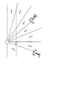
Figure 3: Michel’s monopole solution [66] in which the energy release is due to the electromagnetic energy flux at a null frequency (dark arrows). Light arrows indicate the direction of electric currents.

Very important results have also been obtained in the theory of pulsar magnetospheres and pulsar wind. First of all, Mestel [60], Michel [61], Okamoto [62], and many others (see, e.g., [63, 64]) formulated an axisymmetric force-free ‘pulsar equation’ for the magnetic flux $\Psi(r_{\perp},z)$

$$-\left(1-\frac{\Omega_{\rm F}^{2}r_{\perp}^{2}}{c^{2}}\right)\nabla^{2}\Psi+\frac{2}{r_{\perp}}\frac{\partial\Psi}{\partial r_{\perp}}-\frac{16\pi^{2}}{c^{2}}I\frac{{\rm d}I}{{\rm d}\Psi}$$

$$+\frac{r_{\perp}^{2}}{c^{2}}\left(\nabla\Psi\right)^{2}\Omega_{\rm F}\frac{{\rm d}\Omega_{\rm F}}{{\rm d}\Psi}=0,$$ (32)

where the total electric current within the tube $I(\Psi)$ and the angular velocity $\Omega_{\rm F}(\Psi)$ determining the electric field

$${\bf E}=-\frac{\Omega_{\rm F}}{2\pi c}\,\nabla\Psi$$

depend on the magnetic flux only. This nonlinear equation with a singularity at the light cylinder allowed determining the magnetic field structure because

$${\bf B}_{\rm p}=\frac{[\nabla\Psi\times{\bf e}_{\rm\varphi}]}{2\pi r_{\perp}}.$$

Therefore, it is not surprising that this equation established itself for many years as the main tool in theoretical studies of radio pulsars.

In particular, one of the analytic solutions, which could be obtained only for a very special class of the functions $I(\Psi)$ and $\Omega_{\rm F}(\Psi)$ determining the poloidal current density $j_{\parallel}=j_{\rm GJ}$ and the electric field ${\bf E}$ showed that a monopole solution can be constructed for the Goldreich current $j_{\parallel}=j_{\rm GJ}$ with the electric field being lower than the magnetic field up to infinity [66]:

$$B_{r} = B_{\rm L}\frac{R_{\rm L}^{2}}{r^{2}},$$ (33)

$$B_{\varphi} = E_{\theta}=-B_{\rm L}\,\frac{\Omega R_{\rm L}^{2}}{cr}\,\sin\theta.$$ (34)

Here, $B_{\rm L}=B_{0}(\Omega R/c)^{3}$ is the magnetic field on the light cylinder, and we present the solution in the upper half-plane. The longitudinal current exactly corresponds to a purely radial motion of massless particles with the speed of light:

$$j_{r}=\rho_{\rm GJ}c=-\frac{\Omega B_{\rm L}}{2\pi}\,\frac{R_{\rm L}^{2}}{r^{2}}\,|\cos\theta|.$$ (35)

As shown in Fig. 3, in this solution the longitudinal electric currents (contour arrows) generate a toroidal magnetic field $B_{\varphi}$, which together with the induction electric field $E_{\theta}$ induced by rotation forms a radial electromagnetic energy flux (Poynting vector)

$$S_{r}=\frac{B_{\rm L}^{2}\Omega^{2}R_{\rm L}^{4}}{4\pi cr^{2}}\sin^{2}\theta,$$ (36)

that carries energy away from the neutron star. Thus, the possibility of a magneto-hydrodynamic wind leading to the neutron star spin-down was demonstrated.

We emphasize that all energy losses for such an axisymmetric (and stationary) force-free solution are related to the Poynting vector flux. However, in contrast to a magnetodipole wave, the energy flux occurs at the zero frequency. Of course, the presence of an equatorial current sheet separating the incoming and outgoing magnetic field fluxes appeared to be rather artificial initially. However, as we see in what follows, this solution played a fundamental role in later investigations.

On the other hand, our group (Beskin, Gurevich, and Istomin (BGI) [67]) obtained an analytic solution for an oblique rotator, but for a zero longitudinal electric current in the neutron star magnetosphere (Fig. 4a). In this case, energy losses were shown to be zero for any angle $\chi$ because, for a zero longitudinal current, the condition $B_{\varphi}(R_{\rm L},z)=0$ must hold on the light cylinder for any inclination angle. This effect, later confirmed by Mestel’s group [68] (Fig. 4b) occurs because the plasma filling the neutron star magnetosphere fully screens the magnetodipole radiation of the central star. Therefore, all energy losses must be related to the braking torque ${\bf K}$ caused by the action of the longitudinal currents in the neutron star magnetosphere.

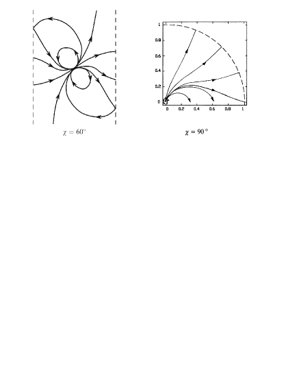
Figure 4: Structure of magnetic field lines for an oblique rotator with a null longitudinal current for the angles (a) $\chi=60^{\circ}$ ($xz$ plane) [67] and (b) $\chi=90^{\circ}$ ($xy$ plane) [68].

It is convenient in what follows to decompose the braking torque ${\bf K}$ into two components, parallel and perpendicular to the magnetic dipole ${\bf m}$. We also introduce the dimensionless current density $i=j_{\parallel}/j_{\rm GJ}$, and decompose it into the symmetric and antisymmetric components $i_{\rm s}$ and $i_{\rm a}$, depending on whether the corresponding component has the same or different sign in the north and south parts of the polar cap. It is easy to verify that $K_{\parallel}\propto i_{\rm s}$ and $K_{\perp}\propto i_{\rm a}$. Here and below, we normalize it to the ‘local’ Goldreich current density $j_{\rm GJ}=|{\bf\Omega}\cdot{\bf B}|/2\pi$. In particular, the direct effect on the star of the Ampère force ${\bf K}=\int[{\bf r}\times[{\bf J}_{\rm s}\times{\bf B}]/c]\,{\rm d}s$, due to the surface currents ${\bf J}_{\rm s}$ closing the volume longitudinal currents in the magnetosphere can be written as [69]

$$K_{\parallel}^{\rm cur} \approx -c_{\parallel}\,\frac{B_{0}^{2}\Omega^{3}R^{6}}{c^{3}}i_{\rm s},$$ (37)

$$K_{\perp}^{\rm cur} \approx -c_{\perp}\,\frac{B_{0}^{2}\Omega^{3}R^{6}}{c^{3}}\left(\frac{\Omega R}{c}\right)i_{\rm a}.$$ (38)

Here, the coefficients $c_{\parallel}\approx 1$ and $c_{\perp}\approx 1$ (which we do not discuss in what follows) depend on the actual current distribution in the open line volume. For the ‘local’ Goldreich current ($i_{\rm s}=i_{\rm a}=1$), Eqn (38) yields

$$K_{\perp}^{\rm cur}\approx\left(\Omega R/c\right)K_{\parallel}^{\rm cur}.$$ (39)

Returning to the evolution of the angular velocity $\Omega$ and the inclination angle $\chi$, we can write the equations of motion in the general form [69, 70]

$$I_{\rm r}\,\dot{\Omega} = K_{\parallel}^{\rm A}+(K_{\perp}^{\rm A}-K_{\parallel}^{\rm A})\sin^{2}\chi,$$ (40)

$$I_{\rm r}\,\Omega\,{\dot{\chi}} = (K_{\perp}^{\rm A}-K_{\parallel}^{\rm A})\sin\chi\cos\chi,$$ (41)

where, again, $I_{\rm r}\sim MR^{2}$ is the neutron star moment of inertia, and we set $K_{\parallel}=K_{\parallel}^{\rm A}\cos\chi$ and $K_{\perp}=K_{\perp}^{\rm A}\sin\chi$. Clearly, both equations involve the factor $(K_{\perp}^{\rm A}-K_{\parallel}^{\rm A})$, and therefore the angle $\chi$ evolves to $90^{\circ}$ (counter-alignment) if the total energy losses decrease at large inclination angles and to zero (alignment) otherwise. For example, for the local Goldreich current ($i_{\rm s}^{A}=i_{\rm a}^{A}=1$), as assumed in the BGI model [69], the angle $\chi$ increases with time:

$$W_{\rm tot}^{({\rm BGI})}=i_{\rm s}^{\rm A}(\Omega,B_{0},\chi)\,\frac{f_{\ast}^{2}(\chi)}{4}\,\frac{B_{0}^{2}\Omega^{4}R^{6}}{c^{3}}\,\cos^{2}\chi,$$ (42)

$${\dot{\chi}}^{({\rm BGI})}=i_{\rm s}^{\rm A}(\Omega,B_{0},\chi)\,\frac{f_{\ast}^{2}(\chi)}{4I_{\rm r}}\,\frac{B_{0}^{2}\Omega^{2}R^{6}}{c^{2}}\sin\chi\,\cos\chi.$$ (43)

Here, the dimensionless factor $1.59<f_{\ast}(\chi)<1.96$ determines the polar cap area $s(\chi)$,

$$s(\chi)=f_{\ast}(\chi)\pi R_{0}^{2}.$$ (44)

As regards the dimensionless currents $i_{\rm a}^{\rm A}(\Omega,B_{0},\chi)$ and $i_{\rm s}^{\rm A}(\Omega,B_{0},\chi)$, we consider them in more detail in Sections 2.2.1 and 3.1.1 below.

As we see, already in the first years, the main processes responsible for the evolution of radio pulsars were understood and the main laws describing pulsar magnetospheres were formulated. Moreover, several analytic solutions enabling the first cautious predictions were obtained. Apparently, all the remaining problems were to be fully clarified quite soon.

Unfortunately, that did not happen. Due to the absence of any significant progress in solving nonlinear equations describing pulsar magnetospheres (analytic solutions could be obtained only in some model cases, and numerical methods were not sufficiently developed at that time), the number of astrophysicists actively working in this field sharply decreased. Difficult times had come.

1.4 Dark ages (1983–1999)

This was a hard time indeed, especially for the theory of radio pulsar magnetospheres. At first glance, no significant results were obtained in the field in these 15 years. However, slowly, step by step, our understanding of processes in neutron star magnetospheres was becoming more and more clear.

First of all, important results were obtained in the theory of strongly magnetized pulsar wind. We recall that the force-free approximation (i.e., the approximation postulating the vanishing of only the electromagnetic force) suggests nothing about the outflowing plasma energy, because such an approximation is equivalent to massless particles. Therefore, in this period, a full MHD theory of relativistic and nonrelativistic flows was actively being developed [71-76]. In particular, this theory showed that the acceleration of particles must be strongly suppressed in a quasi-spherical magnetized wind. As first shown by Tomimatsu in 1994 [77], at long distances (more precisely, beyond the fast magnetosonic surface, $r\gg r_{\rm F}$, where $r_{\rm F}\sim\sigma_{\rm M}^{1/3}\,R_{\rm L}$), the particle energy cannot exceed $\sigma_{\rm M}^{1/3}\,m_{\rm e}c^{2}\sim 1$–$10$ GeV, and hence the electromagnetic-to-particle energy flux ratio $\sigma=W_{\rm em}/W_{\rm part}$ must be high: $\sigma\sim\sigma_{\rm M}^{2/3}\gg 1$.

Simultaneously, it was realized that the longitudinal electric current density $j_{\parallel}$, as well as the accretion rate in the Bondi solution, is not a free parameter but is fixed by the critical conditions on the fast magnetosonic surface. In the relativistic case, the longitudinal current density must be close to the Goldreich current density $j_{\rm GJ}$. Another step forward was related to the recognition of the significant role played by general-relativity effects in the process of particle generation near the neutron star magnetic poles. Mathematically, they are due to an additional term appearing in the expression for the Goldreich-Julian charge density

$$\rho_{\rm GJ}\approx-\frac{(\Omega-\omega)B}{2\pi\,c},$$

related to the Lense-Thirring angular velocity $\omega$

$$\omega\approx\frac{2GI_{r}}{c^{2}\,r^{3}}\,\Omega.$$ (45)

According to general relativity, this is the angular velocity of the spacetime ‘drag’ at a distance $r$ from any rotating body. Despite the smallness of this quantity, its spatial derivative could be sufficiently large. As shown in 1990 in [78] (and later in [79, 80]), in the Arons model, secondary plasma generation becomes possible inside the entire polar cap precisely due to general relativity effects.

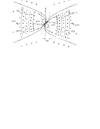
Figure 5: Model of the ‘striped’ pulsar wind with a wave-like current sheet separating oppositely directed magnetic fluxes in the equatorial plane [84].

Here, we also note papers [81-83], which showed that particle creation in the inner gap should be significantly affected by the inverse Compton scattering of thermal photons from the neutron star surface on the relativistic electrons and positrons that are accelerated inside the gap. Hard gamma quanta generated in this process should also lead to single-photon pair creation. Presently, this process is taken into account in most of the works devoted to particle creation near the pulsar surface.

Next, important results were obtained in the pulsar wind theory. First of all, Coroniti [84] and Michel [85] drew attention to a wave-like (striped) current sheet that must arise in a strongly magnetized wind from an oblique rotator by separating the incoming and outgoing magnetic fluxes (Fig. 5). Later, Kennel and Coroniti [86, 87], by analyzing pulsar wind interaction with the Crab Nebula, concluded that at long distances fromthe pulsar, comparable to the size of the nebula, the wind magnetization should be very weak: $\sigma\sim 10^{-2}$. This result was already in direct contradiction with the pulsar wind theory predictions discussed above. Since then, the ‘$\sigma$-problem’, i.e., the impossibility of sufficiently efficient particle acceleration in quasi-spherical flows, has become one of the major problems in the radio pulsar theory. In any case, in the MHD approximation, it remains unsolved so far.

Figure 6: First ‘crazy’ idea [88]: the ‘disk-dome’ model of an axisymmetric magnetosphere. Solid lines show the equipotential electric surfaces, dashed lines are magnetic surfaces.

As usual in difficult times, several ‘crazy’ ideas were proposed to solve a heap of problems (Figs 6 and 7). First, Michel and Krause-Polsdorff [88] considered the so-called ‘disk-dome’ structure of the axisymmetric pulsar magnetosphere, in which positive and negative charges are captured in different parts of the neutron star magnetosphere separated by vacuum gaps. At first glance, it was totally unclear how such a structure could be stable when taking secondary particle creation into account. However, later, as we see in what follows, this structure was indeed reproduced in numerical simulations.

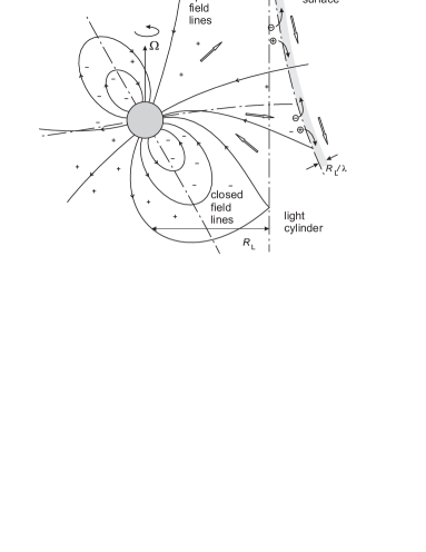
Figure 7: Second ‘crazy’ idea [69]: a model of the magnetosphere with the light surface near which, in a narrow layer $\sim R_{\rm L}/\lambda$, effective particle acceleration occurs. Light arrows show the direction of electric currents; pluses and minuses are the signs of the electric charge density.

In addition, our group considered the case where the longitudinal current $j_{\parallel}$ is small enough to sustain the MHD flow up to infinity [69]. In this model, shown in Fig. 7, the pulsar magnetosphere must have a ‘natural boundary’ — a light surface at which the electric field becomes equal to the magnetic field. This enables effective particle acceleration up to energies ${\cal E}_{\rm e}\approx\sigma_{\rm M}m_{\rm e}c^{2}$ (here, the $\sigma$-problem is solved as well!); as we see in what follows, this conclusion was also later confirmed, albeit indirectly.

We stress that such a structure should inevitably arise in the Arons model, which postulates a ‘local’ Goldreich longitudinal current $j_{\parallel}=c\rho_{\rm GJ}\approx\Omega B\cos\chi/2\pi$, i.e., a longitudinal current that is insufficient to sustain the pulsar wind. Indeed, as discussed in Section 1.3 (see Fig. 3), in the MHD wind, the toroidal magnetic field $B_{\varphi}$ should match the electric field on the light cylinder. But for an oblique rotator, the local Goldreich longitudinal current is too small to create the necessary toroidal magnetic field. As a result, in the BGI model, a weakly magnetized wind, i.e., a flow with low $\sigma$, should be formed already close to the light cylinder.

1.5 Renaissance (1999–2006)

The Renaissance epoch started from two papers published in 1999 and is related to the recognition of the validity of simple models that had already been proposed to explain processes in pulsar magnetospheres. In the first paper, Contopoulos, Kazanas, and Fendt [91] finally solved force-free ‘pulsar equation’ (32) for an axisymmetric magnetosphere numerically (Fig. 8). This became possible due to an iterative procedure to avoid the light cylinder singularity (we already stressed that the light cylinder is a singular surface for the pulsar equation).

As a result, as in the monopole Michel solution, the solution contained an equatorial current sheet at long distances $r>R_{\rm L}$. But in the inner regions, the solution, naturally, was matched to the dipole magnetic field of the neutron star. Several years later, this solution was reproduced in many studies [92-99], which renewed interest in the theory of pulsar magnetospheres. Of course, all these solutions corresponded to the axisymmetric case, which still did not allow obtaining the full information on real pulsar magnetospheres,

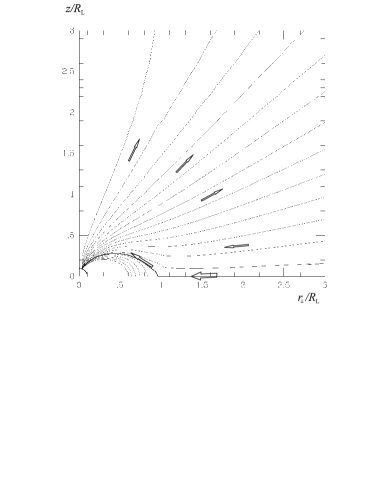
Figure 8: Axisymmetric force-free solution found numerically in [91]. Light arrows show the direction of electric currents.

In the same 1999, Bogovalov [100] found an analytic solution for the so-called ‘inclined split monopole’ (Fig. 9):

$$B_{r} = B_{\rm L}\frac{R_{\rm L}^{2}}{r^{2}}\,{\rm Sign}(\Phi),$$ (46)

$$B_{\varphi} = E_{\theta}=-B_{\rm L}\,\frac{\Omega R_{\rm L}^{2}}{cr}\,\sin\theta\,{\rm Sign}(\Phi).$$ (47)

In this solution, the current sheet near the neutron star separating radial magnetic fluxes is not orthogonal to the spin axis. The quantity

$$\Phi=\cos\theta\cos\chi-\sin\theta\sin\chi\cos\left(\varphi-\Omega t+\Omega r/c\right),$$ (48)

exactly defines the current sheet form. As a result, near the neutron star, the magnetic field has not a dipole but a monopole structure. However, this simple analytic solution was very important for the pulsar wind. In this solution, inside the cones $\theta<\pi/2-\chi$ and $\pi-\theta<\pi/2-\chi$ around the rotation axis, electromagnetic fields remained time-independent and coincided with the Michel solution shown in Fig. 3. On the other hand, in the equatorial plane, all electromagnetic field components, as assumed before (see Fig. 5), changed sign jump-wise when the current sheet crossed a given point; at all other times, the field remained constant.

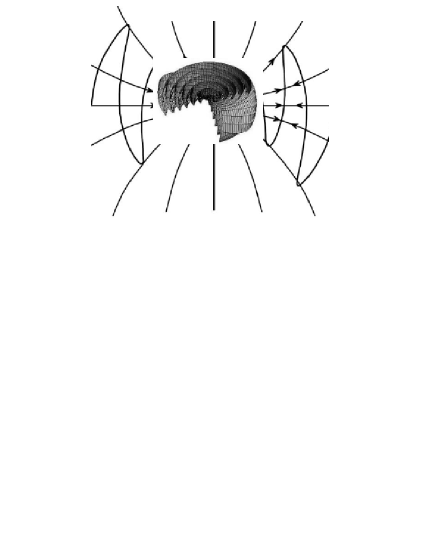
Figure 9: Structure of Bogovalov’s analytic solution for an ‘inclined split monopole’ [100] and the form of the current sheet reproduced on a 3D printer.

We note that the condition $\Phi=0$ for the current sheet form has a purely kinematic nature. This is because in the free-force case, both particles and the current sheet move radially with the speed of light. As a result, in the limit $r\rightarrow\infty$, the relation $E_{\theta}(\theta)=B_{\varphi}(\theta)$ must hold for an arbitrary dependence on the angle $\theta$ for any wind structure; such a stationary asymptotic solution of the ‘pulsar equation’ was first obtained by Ingraham as early as 1973 [101]. Therefore, it is not surprising that a similar structure of the current sheet has been constantly reproduced in subsequent numerical calculations.

Thus, in this time period, real progress was made. First of all, the important role played by the current sheet in the wind dynamics was recognized. Therefore, studies of processes inside the current sheet became the focus of radio pulsar studies. In particular, Lyubarsky and Kirk [102] noted the importance of magnetic reconnection, which initiated many studies. Finally, almost all papers considering an axisymmetric magnetosphere confirmed the magnetosphere structure obtained in [91], thus suggesting the existence of some ‘universal’ solution.

But the main point was apparently related to the change of the viewpoint on the nature of the longitudinal current. The value of $j_{\parallel}^{({\rm us)}}$ determined from the ‘universal solution’ rather than defined by the particle creation process near magnetic poles was now taken as the true longitudinal electric current. In other words, in all subsequent numerical calculations, no constraints on the longitudinal electric current amplitude were imposed. If the particle density in some region became too low in the MHD approach, plasma was injected into that region artificially. It is not surprising therefore that all solutions obtained in this way satisfied both conditions $\rho_{\rm e}=\rho_{\rm GJ}$ and $j_{\parallel}=j_{\parallel}^{({\rm us)}}$.

On the other hand, new questions arose. First of all, the spatial distribution of the longitudinal current $j_{\parallel}$ following from the ’universal solution’ was significantly different from the local Goldreich-Julian current, which, as we especially mentioned above, was predicted by the Arons model. Nor did this distribution match the current from a rotating split monopole. In particular, as shown in Fig. 8, the ‘universal solution’ obtained for an axisymmetric magnetosphere required the inverse current to flow not only along the separatrix separating the closed and open magnetic field lines but also in a sizeable volume outside it. This directly contradicted all models of particle creation near magnetic poles that existed at that time, because, in this case, the sign of the potential drop and hence the direction of the outflowing current had to be the same over the entire polar cap area.

Although this difficulty was not explicitly discussed at that time, the first attempts to overcome this problem were undertaken. In particular, Shibata [103] and later Beloborodov [104] showed that the secondary plasma creation should be significantly suppressed for a sufficiently small longitudinal current $j_{\parallel}<j_{\rm GJ}$.

1.6 Industrial revolution (2006–2014)

The industrial revolution in the radio pulsar theory was related to the emerging possibility of carrying out 3D time-dependent calculations. Like any revolution, it resolved all accumulated problems in a purely technical way.

This epoch started from the work by Spitkovsky [105], who was the first to obtain a numerical solution for the force-free magnetosphere of an oblique rotator. This was the first 3D solution with the pulsar wind outflowing to infinity. As shown in Fig. 10, despite the relative smallness of the computation domain, this solution confirmed the existence of the current sheet.

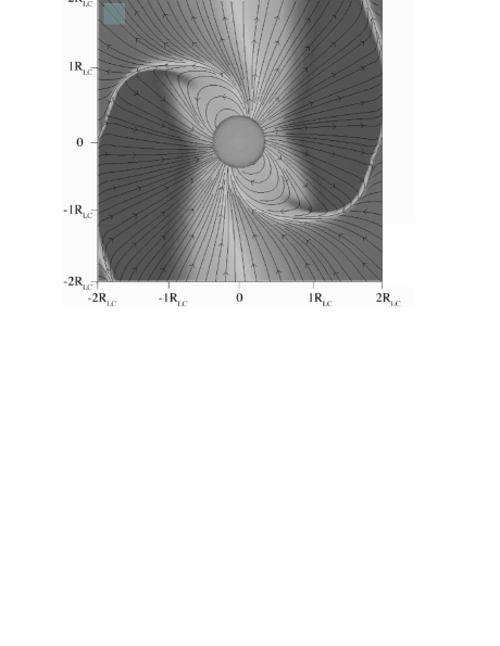
Figure 10: Structure of magnetic field lines in Spitkovsky’s force-free solution [105] for an oblique rotator ($\chi=60^{\circ}$) in the $xz$ plane.

As is well known, an industrial revolution is impossible in one individual country. After Spitkovsky’s work, similar calculations were performed in many research centers, and not only in the force-free but also in the full MHD approximation [106-111]. As a result, the ‘universal solution’ was also found for an oblique rotator, which, in particular, confirmed the formula for the total energy losses obtained by Spitkovsky:

$$W_{\rm tot}^{({\rm MHD})}\approx\frac{1}{4}\,\frac{B_{0}^{2}\Omega^{4}R^{6}}{c^{3}}\,(1+\sin^{2}\chi).$$ (49)

We see that the ‘universal solution’ suggests an increase in losses with the angle $\chi$. Therefore, according to general relation (41), the inclination angle should decrease with time:

$${\dot{\chi}}^{({\rm MHD})}\approx-\frac{1}{4I_{\rm r}}\frac{B_{0}^{2}\Omega^{2}R^{6}}{c^{2}}\sin\chi\,\cos\chi$$ (50)

(this result was obtained somewhat later).

Figure 11: MHD solution [112] demonstrating the magnetic field line concentration ($r=6\,R_{\rm L}$) in the direction at an angle of approximately $30^{\circ}$ to the magnetic axis (the light star).

On the other hand, the ‘universal solution’ was shown to significantly differ from Michel-Bogovalov monopole solution (47). Notably, for sufficiently large angles $\chi>30^{\circ}$, the radial magnetic field was not homogeneous but concentrated near the equatorial plane. The fields averaged over the angle $\varphi$ had the form

$$<B_{r}>_{\varphi} \approx B_{\rm L}\frac{R_{\rm L}^{2}}{r^{2}}\,\sin\theta\,{\rm Sign}(\Phi),$$ (51)

$$<B_{\varphi}>_{\varphi} = <E_{\theta}>_{\varphi}$$ (52)

$$\approx-B_{\rm L}\,\frac{\Omega R_{\rm L}^{2}}{cr}\,\sin^{2}\theta\,{\rm Sign}(\Phi),$$

$$<S_{r}>_{\varphi} \approx \frac{B_{\rm L}^{2}\Omega^{2}R_{\rm L}^{4}}{4\pi cr^{2}}\sin^{4}\theta,$$ (53)

whereas in the Michel-Bogovalov solution the radial magnetic field $B_{r}=B_{\rm L}(R_{\rm L}^{2}/r^{2})\,{\rm Sign}(\Phi)$ in (47) does not depend on the angle $\theta$.

We stress that the fields in Eqns (51)-(53) are averaged over the angle $\varphi$. In fact, as shown in Fig. 11, there is a noticeable concentration of the force lines (and hence the electromagnetic energy flux) in the direction rotated longitudinally through approximately $30^{\circ}$ relative to the magnetic axis (the light star) [107, 112]. Thus, the magnetic field is not time-independent between the current sheet crossings of a given point. Moreover, for large angles $\chi$, the current sheet becomes more and more pronounced, and hence the asymptotic solution for an orthogonal rotator can be approximated with good accuracy as

$$B_{r} \approx B_{\rm L}\frac{R_{\rm L}^{2}}{r^{2}}\,\sin\theta\cos(\varphi-\Omega t+\Omega r/c-\varphi_{0}),$$ (54)

$$B_{\varphi} = E_{\theta}$$

$$\approx -B_{\rm L}\,\frac{\Omega R_{\rm L}^{2}}{cr}\,\sin^{2}\theta\,\cos(\varphi-\Omega t+\Omega r/c-\varphi_{0})$$

(where $\varphi_{0}\approx 30^{\circ}$). This is another significant difference from the Michel-Bogovalov solution, in which, as follows from (47) suggests, the electromagnetic fields are time-independent outside the current sheet. In Section 2.3.1, we discuss the nature of such a pulsar wind in detail, emphasizing its variability.

As noted above, asymptotic solutions with an arbitrary dependence on the angle $\theta$ have been known since the 1970s. Surprising, however, was the fact that these simple solutions were reproduced in three-dimensional MHD simulations. In particular, the general relation between the energy flux averaged over the angle $\varphi$ and the radial magnetic field

$$S_{r}(\theta)\propto B_{r}^{2}(\theta)\,\sin^{2}\theta$$ (56)

holds with good accuracy (it can be easily obtained using the definitions of the ${\bf E}$ and ${\bf B}$ fields).

In addition, an analysis of the obtained solutions shows that the dimensionless antisymmetric longitudinal current significantly exceeds the local Goldreich current: $i_{\rm a}^{\rm A}\sim(\Omega R/c)^{-1/2}\gg 1$ (see Section 2.2.1 for more details). Due to the normalization introduced above, this means that the total current circulating in the magnetosphere of an oblique rotator is close to the total current flowing in an axisymmetric magnetosphere. This should be the case because, independently of the angle $\chi$, for the MHD wind outgoing to infinity to exist, the toroidal magnetic field on the light cylinder $B_{\varphi}(R_{\rm L})$ should be close to the poloidal field $B_{\rm p}(R_{\rm L})$. This implies that the total current $I$ should be weakly dependent on $\chi$.

On the other hand, we stress that the value of this current is insufficient to explain the energy losses in the ‘universal solution’ (49) for $\chi\approx 90^{\circ}$ only due to volume currents circulating in the magnetosphere. Indeed, according to Eqn (38), this requires the antisymmetric current to be much larger: $i_{\rm a}^{\rm A}\sim(\Omega R/c)$. Of course, we must not forget that in all numerical calculations, the neutron star size was not less than 10% of the light cylinder radius (for ordinary pulsars, this value is hundredths of a percent). However, no significant dependence of the pulsar wind parameters on the stellar size was found. Anyway, the problem of the pulsar braking mechanism remained unsolved.

At the same time, a novel view on the role of the ‘universal current’ allowed Timokhin [113] (and later Timokhin and Arons [114]) to numerically simulate the process of particle creation near magnetic poles, for the first time including the possible nonstationarity of this process. The longitudinal current $j_{\parallel}^{({\rm us)}}$ was regarded as an external constant parameter. Pair creation was shown to be possible for a sufficiently large longitudinal current $j_{\parallel}>j_{\rm GJ}$ and, as already obtained earlier [103, 104], impossible for lower currents. Moreover, particle creation was shown to occur in the inverse current region at the main magnetic field feet near the separatrix; in this case, the plasma density in the generation region should be not lower but higher than the Goldreich-Julian charge density. This becomes possible exactly because the particle creation is essentially nonstationary.

Here, however, we note that these calculations assumed one-dimensional plasma flow, and this did not allow believing that all essential points are taken into account. For example, the change in the toroidal magnetic field was ignored, which, as was shown already a long time ago [36], could significantly affect the plasma generation dynamics (see the Appendix). Nevertheless, these papers significantly contributed to the understanding of the very possibility of generation of the required longitudinal current, which is significantly different from the local Goldreich current. Here, in fact, we returned to the Ruderman-Sutherland model [115] because, despite the free particle ejection from the surface, the electric potential drop in the particle generation region turns out to be much larger than in the Arons model.

Summarizing, we can conclude that the ‘industrial revolution’ enabled a leap forward in the understanding of the basic processes occurring in pulsar magnetospheres. It is very important that most of the results were confirmed by different research groups. Nevertheless, some key questions remained unanswered. One of the main issues was whether particle generation provides the necessary longitudinal current $j_{\parallel}^{({\rm us)}}$ determined by the ‘universal solution’. For example, for an orthogonal rotator (and for a period $P\sim$ 1 s), the longitudinal current should be $(\Omega R/c)^{-1/2}\sim 100$ times as high as the local Goldreich current; this high parameter had not been used in numerical simulations.

1.7 Modern times (after 2014)

Formally, this is just the next stage in the numerical simulations related to the use of the particle-in-cell (PIC) method. In fact, a qualitative step forward has been made, because the kinetic treatment alone, unlike one-fluid MHD and moreover the force-free case, enabled self-consistently extending the models to particle generation, i.e., to a systematic description of both the region with the longitudinal electric field $E_{\parallel}$ and the particle injection into the calculation domain. This, in addition, enabled the description of particle acceleration beyond the light cylinder (during the ‘industrial revolution’ time, these effects were modeled by introducing an effective resistance [116, 117]). In other words, PIC simulations allowed ab initio calculations, at least in principle [118].

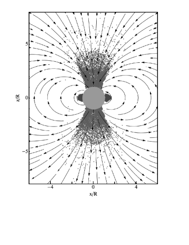
Figure 12: First PIC calculation results: axisymmetric magnetosphere ignoring general relativistic effects [119].

Of course, this epoch, in fact, has just begun, and therefore not all results mentioned below have been tested in independent calculations. Nevertheless, despite ‘teething problems’ (natural in this case), the new possibilities offered by this method have already given several interesting results.

These studies started from two papers by Philippov and Spitkovsky [119] and by Chen and Beloborodov [120] (see also [121]). Their primary focus was on testing whether, in the absence of particle generation in the magnetosphere (i.e., only for free ejection of particles from the neutron star surface), no magnetized pulsar wind arises, but the ‘disk-dome’ structure we already discussed in Section 1.4 is formed (Fig. 12). The force-free solution with pulsar wind arose only if the particle generation occurred inside the total magnetosphere volume.

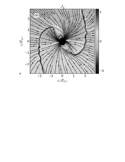
Figure 13: First PIC calculation results: the structure of magnetic field lines for an oblique rotator [122].

Next, Philippov, Spitkovsky, and Cerutti [122], using a more realistic particle creation model, reproduced the structure obtained in the MHD simulations. In particular, as shown in Fig. 13, they confirmed the existence of the current sheet. Thus, the existence of the ‘universal solution’ was also checked. In addition, effective particle acceleration beyond the light cylinder to maximal energies $\gamma\approx\sigma_{\rm M}$ was shown to be possible [123, 124]. This process was made possible exactly because of the appearance of regions where the electric field exceeds the magnetic one (which is related to the decrease in the magnetic field inside the equatorial current sheet). Another reason for which particle acceleration turns out to be effective is the magnetic reconnection, because the electric field arising in this process leads to particle drift toward the current sheet.

As a result, according to the authors of [122], already at short distances $r<5\,R_{\rm L}$ from the light cylinder, up to 30% of the total electromagnetic energy of the wind is transferred to the particles. However, it is currently difficult to say whether this solves the $\sigma$-problem; nonetheless, a certain step forward has undoubtedly been made. In any case, such effective particle acceleration should definitely help to explain the high-energy radiation from pulsars detected by the Fermi gamma-ray observatory [125].

On the other hand, kinetic calculations posed more new questions than produced answers. Indeed, already the first results obtained in [119, 120] for an axisymmetric magnetosphere unexpectedly showed the lack of particle generation near magnetic poles. Instead, as shown in Fig. 12, the free particle ejection from the neutron star surface (which, we recall, is postulated in the calculations!) leads not to the ‘universal solution’ but to the appearance of the ‘disk-dome’ structure mentioned above. Later, such a solution was shown to also appear for not very large angles $\chi<30^{\circ}$. This effect is directly related to the required longitudinal current $j_{\parallel}^{({\rm us})}$ being less than $\chi<30^{\circ}$; as mentioned in Section 1.4, no particle generation occurs in this case. Fortunately, this problem was successfully solved very soon afterwards [118]. It turned out that the general relativity effects (which, as we know, change the Goldreich-Julian charge density) lead to the reversal of the inequality ($j_{\parallel}^{({\rm us})}>j_{\rm GJ}$), which enabled the particle generation process. As a result, as shown in Fig. 13, the ‘universal solution’ was generally reproduced in the framework of this approach.

A second, more serious, problem proved to be connected to the inverse current formation. By the present time, this current has been obtained or the fastest radio pulsars only, in which electromagnetic fields and article densities near the light cylinder are high enough for secondary lectron-positron plasma generation. In other words, presently, it is ot possible to close the current (and hence to provide the ‘universal olution’) without additional particle creation beyond the light cylinder. In this case, as is also shown in [119, 120], a ‘disk-dome’ like structure appears.

One way or another, studies in this field actively continue, and we can hope that many points will be clarified in the nearest future.

2 Several awkward questions

2.1 Old and forgotten…

Success in studies of radio pulsar magnetospheres achieved in the last several years is quite impressive. Nevertheless, we should not forget that many explicit and implicit assumptions have been adopted in numerical simulations, which undoubtedly affect the generality of the results obtained. This especially relates to PIC simulations because, in fact, these calculations have just begun.

On the other hand, there are several questions that the author remembers from as early as the mid-1970s and which have not received reasonable answers so far. These, of course, include one of the principal questions of the radio pulsar theory: the question of the nature of coherent radio emission. Because of a lack of space, we do not consider it. But it is also impossible to ignore it among other unsolved issues.

Unfortunately, many of these questions are barely discussed now, although the corresponding theoretical and observational studies, in our opinion, would enable significant progress in the understanding of radio pulsar activity. Even more regrettable is the fact that radio pulsar observers are not inclined to carry out test studies to check the predictions of the theory.

2.1.1 Axis orientation.

If we take virtually any catalogue with data on the inclination angle $\chi$ between the magnetic and rotation axes [24, 126-128], we discover that this angle lies in the range $0^{\circ}$–$90^{\circ}$. Of course, this by no means implies that there are no radio pulsars with the inclination angle $\chi$ in the range $90^{\circ}$–$180^{\circ}$. This is simply because most of the existing methods for determining this angle do not distinguish between $\chi$ and $180^{\circ}-\chi$. Only additional information, for example, from X-ray and gamma-ray observations, allows estimating the inclination angle in the entire possible range [129-133].

On the other hand, from the physical standpoint, acute and obtuse angles between the axes correspond to two principally different conditions because for small $\chi$, the longitudinal current outflowing from the polar cap area (with its sign determined by the sign of the Goldreich-Julian charge density $\rho_{\rm GJ}=-{\bf\Omega}\cdot{\bf B}/2\pi c$) corresponds to negative charges, whereas for angles $\chi$ exceeding $90^{\circ}$ it corresponds to positive ones. Clearly in the models of secondary plasma generation in which the particle ejection from the neutron star surface is important, these are two essentially different cases, at least because the work function of positive charges must be different from that of electrons. Indeed, the ejection of ions, and not positrons, which are absent in the neutron star crust, should be considered here. As we have seen, this relates to the Arons model first and foremost; in the Ruderman-Sutherland model, the particle creation is insensitive to the axis orientation.

Therefore, one of the most interesting questions actually facing the radio pulsar theory is understanding whether the necessary secondary electron-positron plasma generation can occur for arbitrary angles. If it is proved, as was shown in recent paper [133] using a small sampling of 26 pulsars, that the number of radio pulsars with inclination angles $\chi<90^{\circ}$ is approximately equal to that with inclination angles $\chi>90^{\circ}$ (with the properties of radio emission showing no sign of separation into two groups), then it might be possible to conclude that particle ejection is hardly significant for the secondary electron-positron plasma generation.

As stressed in Section 1.7, all numerical calculations of pulsar magnetospheres carried out in recent years have assumed the free particle ejection, i.e., a sufficiently small work function $A_{\rm w}$. However, this also remains an open issue. The point is not only in the accuracy achieved so far in determining the work function [134, 135]; it turned out that the chemical composition of the neutron star surface layer is unknown: it may not consist of iron atoms, as most studies have assumed.

The chemical composition of the surface layers of the polar caps can significantly change due to their bombardment by energetic particles accelerated by the longitudinal electric field in the inner gap. In addition, according to [136], iron atoms (which certainly are produced in the largest numbers because they have the most stable nuclei) could ‘sink down’ in the gravitational field in the first several years after the neutron star birth, when its surface is undoubtedly not solid. Therefore, it is not ruled out that, in fact, the neutron star surface layers consist of not iron but much lighter atoms like hydrogen and helium. But because the melting temperature, which can be roughly estimated by the formula [137]

$$T_{\rm m}\approx 3.4\times 10^{7}Z_{26}^{5/3}\,\rho_{6}$$ (57)

(where $\rho_{6}$ is the surface layer density in units $10^{6}$ g cm^-3 and $Z_{26}=Z/26$ depends on the atomic number $Z$, the neutron star surface at a temperature $\sim 10^{6}$K, which is typical of ordinary radio pulsars, should be liquid and, in any case, should not prevent free particle ejection. Modern models of thermal emission of radio pulsars are based just on this picture [138, 139].

2.1.2 Surface heating.

The surface heating problem is also an old and very interesting question. As we noted above, in the 1960s, the smallness of the neutron star surface was one of the reasons why dedicated searches for them were not undertaken. Presently, the sensitivity of space X-ray telescopes enables successful observations of both accreting X-ray pulsars and proper thermal emission from the nearest isolated neutron stars. Thermal emission has been detected not only from ‘active’ radio pulsars but also from neutron stars that do not demonstrate radio emission for some reason [140-142].

We do not discuss the problems related to the interpretation of spectra here (a super strong magnetic field significantly changes the properties of the atmosphere and surface layers of neutron stars, which essentially distorts the thermal radiation spectrum [139]), but touch upon the total thermal power. Most of the radio pulsars from which thermal radiation is observed were found to have sufficiently small spin periods. With decreasing the spin period $P$, the relative contribution of the X-ray luminosity $L_{\rm X}$ with respect to the total energy losses $W_{\rm tot}$ generally decreases, and for spin periods $P\sim 0.3$ s, the ratio $L_{\rm X}/W_{\rm tot}$ is only a fraction of a percent. Incidentally, this dependence is the complete opposite of the one for gamma-ray emission (for fast radio pulsars, the gamma-ray luminosity is close to the total energy loss of neutron stars). However, this behavior has a quite simple explanation.

Indeed, the obvious heating source of the polar caps (and hence of the entire neutron star) is the flux of secondary particles accelerated in the inner gap directed toward the neutron star. Their total power is proportional to the product of the potential drop $\psi$ by the total flowing current $I$, whereas the full power $W_{\rm tot}$ due to current energy losses is equal to the product $I\psi_{\rm max}$. As we have seen, the ratio $\psi/\psi_{\rm max}$, independently of the particle generation model, decreases as the angular velocity $\Omega$ increases. Thus, the decrease in the ratio $L_{\rm X}/W_{\rm tot}$ with $\Omega$ can be regarded as a confirmation of the heating mechanism due to the inverse particle flux. In any case, thermal emission from neutron stars provides a clear upper bound for this flux.

Polar cap heating can significantly affect the particle ejection rate from the neutron star surface. For example, papers assuming the ejection of positively charged particles, i.e., for angles $\chi>90^{\circ}$ (see, e.g., [143, 144]) typically use the following formula for the thermal current [39]:

$$j(T)=j_{\rm GJ}\,\exp\left(30-\frac{A_{B}}{T}\right)\,T_{\rm keV}^{1/2}\,P\,B_{12}^{-1}\,Z_{26}\,A_{56}^{-3/2}\,\rho_{4},$$ (58)

where $A_{B}$ is the binding energy of ions with the atomic number $A$ and charge $Z$; and $\rho_{4}$ is the surface density in units of $10^{4}$ g cm^-3; of course, this formula is valid only for $j(T)<j_{\rm GJ}$. As we see, the nonlinear exponential dependence of the thermal current $j$ on the temperature $T$ can significantly influence the particle generation rate.

As regards the various models of secondary plasma generation in the inner gap, we note that the original model of secondary plasma generation proposed by Ruderman and Sutherland, in which the longitudinal current is equal to the Goldreich current ($j_{\parallel}\approx j_{\rm GJ}$) and the potential drop in the gap is $\psi\approx\psi_{\rm RS}$, Eqn (21), undoubtedly contradicts the observed surface heating, because in this model the inverse particle flux is comparable to the particle flux outflowing from the pulsar magnetosphere. On the other hand, the Arons model [46], in which the inverse particle flux

$$\frac{j_{\rm back}}{j_{\rm GJ}} \approx \left(\frac{\Omega R}{c}\right)^{1/2}$$ (59)

and potential drop (24) amount to only a fraction of a percent of those in the Ruderman-Sutherland model, could seem to successively solve the surface heating problem. However, as stressed above, this model was rejected for other reasons.

The recent studies devoted to particle generation [113, 114], whose results, as already stressed, are very similar to the results of the Ruderman-Sutherland model, revived the surface heating problem, because for pulsars with sufficiently small periods the surface temperature should be much higher than actually observed. Presently, there is no satisfactory answer to this question.

2.1.3 Account for the potential drop in the ‘inner gap’.

The next question is related to the need to account for the potential $\psi$ drop in the inner gap above the neutron star surface in the pulsar wind region. We recall that in our model (which we consider in Section 3 below), this potential plays a decisive role. However, in numerical simulations (with a possible exception of [113]), the additional potential $\psi$ has never been taken into account. Clearly, this assumption has been based on solid grounds, because for rapidly rotating pulsars, which, in fact, have been the only ones considered so far, the potential drop needed for the secondary plasma generation has always been smaller than the maximum value $\psi_{\rm cmax}$ given by formula (23). But for pulsars located near the ‘death line’, this is clearly not the case, and the potential drop effect can be significant.

Indeed, as was already shown in [29], a nonzero potential $\psi$ in the region of open magnetic lines leads to additional plasma rotation around the magnetic axis (see Fig. 1). For an oblique rotator, this is observed as the subpulse drift phenomenon [145, 146]. A regular drift has already been found in 97 radio pulsars [147]; in 53 of them, subpulses shift in the negative direction relative to the pulse phase $\phi$ and in 44 in the positive direction. An approximate equality should indeed take place for an arbitrary orientation of the observer relative to the magnetic axis.

Everywhere below, we consider a model of an ideally conducting sphere, implying that the freezing-in condition

$${\bf E}_{\rm in}+[{\boldsymbol{\beta}}_{\rm R}\times{\bf B}_{\rm in}]=0.$$ (60)

holds inside the star. Here and below, by definition,

$${\boldsymbol{\beta}}_{\rm R}=\frac{[{\bf\Omega}\times{\bf r}]}{c}.$$ (61)

On the other hand, assuming quasi-stationarity (with the coordinate $\varphi$ and time $t$ entering all expressions only in the combination $\varphi-\Omega t$), the Maxwell equation corresponding to the Faraday law is well known to admit the form $\nabla\times({\bf E}+[{\boldsymbol{\beta}}_{\rm R}\times{\bf B}])=0$ [60], whence

$${\bf E}+[{\boldsymbol{\beta}}_{\rm R}\times{\bf B}]=-\nabla\psi.$$ (62)

This implies that the potential $\psi=0$ inside the sphere, and therefore, above the inner gap in the outflowing plasma region, the potential $\psi$ is exactly equal to the potential drop in the gap itself. In this region, a full screening of the longitudinal electric field component is assumed, whence we have ${\bf{E}}\cdot{\bf B}=0$ there. Taking the scalar product with ${\bf B}$, we then immediately obtain $\nabla\psi\cdot{\bf B}=0$, i.e., the potential $\psi$ is constant along the magnetic field lines.

For illustration, we consider two examples visually showing how the pulsar wind structure can be significantly changed by taking the potential drop in the inner gap into account. We first note that a nonzero potential c alters the Goldreich-Julian charge density (if the latter is understood as the charge density needed to screen the longitudinal electric field). Then, in terms of the dimensionless potential [69]

$$\beta_{0}=\frac{\psi}{\psi_{\rm max}},$$ (63)

we have

$$\rho_{GJ}\approx-(1-\beta_{0})\frac{{\bf\Omega}\cdot{\bf B}}{2\pi c}.$$ (64)

near the neutron star surface. As we see, for pulsars near the ‘death line’, where $\beta_{0}\sim 1$, the Goldreich-Julian charge density (and hence the Goldreich current) significantly decreases. The outgoing electromagnetic energy flux decreases accordingly. For example, in the axisymmetric case,

$$W_{\rm tot}\approx(1-\beta_{0})^{2}W_{\rm tot}^{(0)},$$ (65)

because both the electric and toroidal magnetic fields decrease by the factor $(1-\beta_{0})$. In view of the foregoing, it is not necessary to explain how important this point can be for plasma generation near the neutron star surface.

As another example, we consider a generalization of asymptotic formula (46) for electromagnetic fields in a quasi-radial pulsar wind of an orthogonal rotator:

$$B_{r} \approx B_{\rm L}\frac{R_{\rm L}^{2}}{r^{2}}\,\sin\theta\cos(\varphi-\Omega t+\Omega r/c-\varphi_{0}),$$ (66)

$$B_{\theta} \approx \frac{1}{r\sin\theta}\,\frac{\partial\psi}{\partial\varphi},$$ (67)

$$B_{\varphi} \approx -B_{\rm L}\,\frac{\Omega R_{\rm L}^{2}}{cr}\,\sin^{2}\theta\,\cos(\varphi-\Omega t+\Omega r/c-\varphi_{0})$$ (68)

$$-\frac{1}{r}\,\frac{\partial\psi}{\partial\theta},$$

$$E_{r} \approx 0,$$ (69)

$$E_{\theta} \approx -B_{\rm L}\,\frac{\Omega R_{\rm L}^{2}}{cr}\,\sin^{2}\theta\,\cos(\varphi-\Omega t+\Omega r/c-\varphi_{0})$$ (70)

$$-\frac{1}{r}\,\frac{\partial\psi}{\partial\theta},$$

$$E_{\varphi} \approx -\frac{1}{r\sin\theta}\,\frac{\partial\psi}{\partial\varphi}.$$ (71)

Here,$\psi(\theta,\varphi-\Omega t+\Omega r/c)$ an arbitrary function of two arguments. Now, for example, determining the electromagnetic energy flux for the potential

$$\psi=\beta_{0}\psi_{\rm max}\sin\theta\cos\theta\cos(\varphi-\Omega t-\Omega r/c+\varphi_{0}),$$ (72)

for small $\beta_{0}$ we obtain

$$W_{\rm tot}\approx\left(1-\sqrt{\frac{3}{10}}\beta_{0}\right)W_{\rm tot}^{(0)}.$$ (73)

Therefore, also for an orthogonal rotator with a nonzero potential $\psi$, the energy losses decrease. However, in this case, the value $\psi$ itself cannot exceed $(\Omega R/c)^{1/2}\psi_{\rm max}$ ($\beta_{0}\ll 1$) and therefore the role of the additional potential is insignificant.

2.1.4 Orthogonal pulsars.

To conclude this discussion, we make one more note about a possible avenue of research. Among more than 2600 presently known radio pulsars, there are about 30 sources that are classified as orthogonal rotators due to the presence of an interpulse exactly in the middle of the main pulses. The presence of the interpulse in this case is easily explained by the emission from the opposite magnetic pole. Almost all morphological properties of pulsars with interpulses are indistinguishable from those of ordinary pulsars. The only distinctive feature of these pulsars is their sufficiently small spin periods $P<0.5$ s. This is not surprising because for angles $\chi$ close to $90^{\circ}$, the plasma generation condition $\psi_{\rm RS}(\chi)<\psi_{\rm max}(\chi)$ can be satisfied only for sufficiently small periods $P$ (Fig. 14).

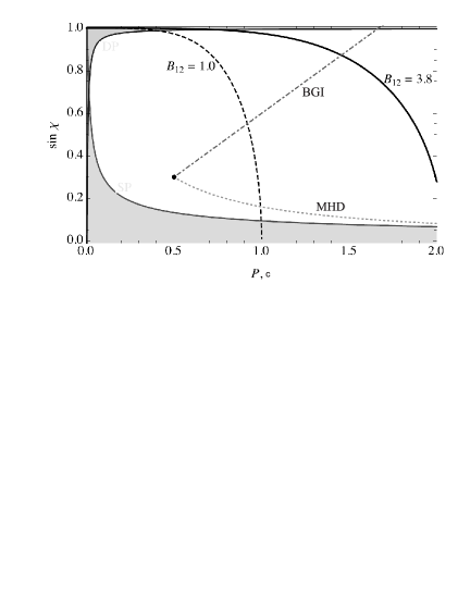
Figure 14: ‘Death line’ as a function of the angle $\chi$ and period $P$ for different values of the magnetic field $B_{0}$ [177]. Also shown are evolutionary trajectories in the ‘universal’ MHD model and the BGI model. Grey color shows regions of possible interpulse observations for almost orthogonal (the upper region) and almost aligned (the bottom region) radio pulsars.

In our opinion, the analysis of interpulse pulsars could greatly help to understand pulsar magnetosphere processes. Indeed, the very existence of orthogonal radio pulsars, whose polarization and other radio emission properties do not differ from those of other pulsars, suggests ‘standard’ particle generation. On the other hand, analysis of polarization properties of their radio emission shows that for these pulsars it is possible to reliably determine the angles $\chi>90^{\circ}$ [148]. As a result, it turned out that the radio emission from some of them is connected to different secondary plasma generation regions, corresponding to positive and negative charge outflows.

2.2 Longitudinal current

2.2.1 ‘Mestel’s’ current.

We reiterate that the key point in the magnetosphere structure is the value of the longitudinal current circulating in the magnetosphere. Therefore, below, we make several notes concerning the procedure for determining this longitudinal current.

Already in the very first years of radio pulsar magnetosphere studies, it became clear that particle motion is mainly determined by the electric drift related to the electric field induced by neutron star rotation. Other drift velocities can be ignored. As a result, the density of the transverse electric current ${\bf j}_{\perp}$ can be written in the hydrodynamic form as ${\bf j}_{\perp}=\rho_{\rm e}{\bf U}_{\rm dr}$ where ${\bf U}_{\rm dr}=c[{\bf E}\times{\bf B}]/B^{2}$ is the electric drift velocity. Such a simple dependence significantly simplified the problem, because the full current in the magnetosphere could be represented simply as ${\bf j}=\rho_{\rm e}{\bf U}_{\rm dr}+a_{\parallel}{\bf B}$, where $a_{\parallel}$ is a scalar function. Using Eqn (62) (and disregarding potential $\psi$), we finally arrive at

$${\bf j}=\rho_{\rm e}[{\bf\Omega}\times{\bf r}]+i_{\parallel}{\bf B},$$ (74)

where $i_{\parallel}$ is another scalar function.

Now, using another Maxwell equation written under the quasi-stationary assumption in the form [60, 67]

$$\nabla\times({\bf B}-[{\boldsymbol{\beta}}_{\rm R}\times{\bf E}])=\frac{4\pi}{c}({\bf j}-c\rho_{\rm e}{\boldsymbol{\beta}}_{\rm R}),$$ (75)

we immediately conclude that $i_{\parallel}$ should be constant along the magnetic field lines: ${\bf B}\cdot\nabla i_{\parallel}=0$. As a result, for the zero potential $\psi$, we obtain

$$\nabla\times[{\bf B}+{\boldsymbol{\beta}}_{\rm R}\times[{\boldsymbol{\beta}}_{\rm R}\times{\bf B}]]=i_{\parallel}{\bf B}.$$ (76)

This is the so-called Mestel equation [60], which is valid, unlike pulsar equation (32), for any angle $\chi$.

In the Hellas and Rome times (1968-1983), the form of the current (74) was very popular because it enabled the determination of the full current using only one additional scalar function $i_{\parallel}$. Moreover, in the axisymmetric case, this was a function of the magnetic flux $\Psi$ only. This equation was also helpful later, when the results of 3D numerical simulations were represented in the form of 2D plots (in such plots, the quantity $i_{\parallel}$ is usually shown in different colors).

Incidentally, exactly such a form enabled the determination of the dimensionless antisymmetric longitudinal current $i_{\rm a}^{\rm A}$, that we discussed in Section 1.7, because the longitudinal current can be easily found in asymptotic solution (54), (55) at $r\gg R_{\rm L}$. Indeed, substituting field expressions (54), (55) for the orthogonal rotator in (75), we immediately obtain

$$i_{\parallel}=-3\,\frac{\Omega}{c}\cos\theta.$$ (77)

Now, comparing the full currents flowing across the upper hemisphere at $r\gg R_{\rm L}$ and through the north part of the polar cap on the neutron star surface, we finally obtain

$$i_{\rm a}^{\rm A}\approx f_{\ast}^{-1/2}\,\left(\frac{\Omega R}{c}\right)^{-1/2},$$ (78)

where we recall that $f_{\ast}\approx 1,96$ is the dimensionless area of the polar cap ($s=f_{\ast}\pi R_{0}^{2}$) for the orthogonal rotator [69].

2.2.2 ‘Gruzinov’s’ current.

On the other hand, Eqn (74) had one essential shortcoming. For an oblique rotator, it was not ‘local’ because the quantity $i_{\parallel}$ at a given point was not expressed through the fields and their derivatives at that point. In numerical simulations, this was important and did not allow fast calculations. This difficulty was overcome in 2005 by Gruzinov [94]. The scalar product of the Maxwell equation $\nabla\times{\bf B}=(1/c)\,\partial{\bf E}/\partial t+(4\pi/c)\,{\bf j}$ with ${\bf B}$ yields the scalar product ${\bf j}\cdot{\bf B}$ as a function of field derivatives. Using the screening condition ${\bf E}\cdot{\bf B}=0$, i.e., replacing ${\bf B}\cdot\partial{\bf E}/\partial t$ with $-{\bf E}\cdot\partial{\bf B}/\partial t$, after simple transformations we finally obtain

$${\bf j}_{\rm G}({\bf E},{\bf B})=$$ (79)

$$\frac{({\bf B}\cdot[\nabla\times{\bf B}]-{\bf E}\cdot[\nabla\times{\bf E}]){\bf B}+(\nabla\cdot{\bf E})[{\bf E}\times{\bf B}]}{B^{2}},$$

where the charge density is expressed via the Maxwell equations $\nabla\cdot{\bf E}=4\pi\rho_{\rm e}$. This form turned out to be very convenient for numerical modeling and is currently in use in all simulations; of course, under certain conditions, the ‘classical’ formulation (74) can be used (see, e.g., [149]).

Indeed, if we now use Eqn (62) (again with $\psi=0$), the quasi-stationary Maxwell equation (75) contains the mag- netic field only:

$$\nabla\times[{\bf B}+{\boldsymbol{\beta}}_{\rm R}\times[{\boldsymbol{\beta}}_{\rm R}\times{\bf B}]]=$$ (80)

$$\frac{4\pi}{c}\,{\bf j}_{\rm G}(-[{\boldsymbol{\beta}}_{\rm R}\times{\bf B}],{\bf B})+(\nabla\cdot[{\boldsymbol{\beta}}_{\rm R}\times{\bf B}])\,{\boldsymbol{\beta}}_{\rm R}.$$

We recall that Eqn (80) remains valid for an oblique rotator. Jointly with the Maxwell equation $\nabla\cdot{\bf B}=0$, they constitute a closed system of equations containing the magnetic field only. Equation (80), of course, is not as compact as Mestel’s equation (76), but it does not contain any scalar functions. Unfortunately, for a nonzero potential $\psi$, the locality is lost again, because the potential $\psi$ cannot be locally expressed through the field derivatives at a given point.

2.3 So how do pulsars spin down?

2.3.1 The last time about magnetodipole losses.

In our opinion, in its initial formulation, this question received a unique and decisive answer long ago: in the magnetosphere of radio pulsars, there are no magnetodipole losses. Nevertheless, magnetodipole losses are frequently invoked when discussing energy losses of radio pulsars. Indeed, because energy losses (49) in the ‘universal solution’ depend on the angle $\chi$ as $(1+\sin^{2}\chi)$ and the addition to unity has the same dependence on $\chi$ as for magnetodipole losses, this would seem to indicate that the magnetodipole contribution can exist.

Numerical simulations carried out in the last decade have not clarified this issue. As we already stressed, Michel-Bogovalov analytic solution (47) certainly does not include a magnetodipole wave because, except for the current sheet crossing moment, the electromagnetic fields are time-independent. However, as shown in Fig. 11, for an orthogonal rotator, there is a noticeable time-dependent field component. Accordingly, there is a significant time dependence in analytic solution (54), (55), which reproduces the pulsar wind from an orthogonal rotator with good accuracy.

Apparently, the correct answer to this question can be formulated as follows. We can speak about magnetodipole radiation if the canonical conditions of the smallness of the emitting region size compared to the wavelength are satisfied, i.e., if there is a wave zone. In the pulsar wind, this condition definitely does not hold, because both charges and currents in situ play a decisive role in the wind structure formation. Indeed, nobody would speak of the magnetodipole radiation of a wire with an alternating current, although the energy transfer outside the wire is exactly due to the electromagnetic energy flux. All this, however, occurs in the near zone, and hence both charges and currents are at distances comparable to the wavelength.

Thus, the pulsar wind should be viewed as an example of a relativistic magnetohydrodynamic wave with unusual properties, which we still know little about. For example, we have seen that the angular distribution of the energy flux changes from $\sin^{2}\theta$ for an axisymmetric rotator to $\sin^{4}\theta$ for an orthogonal one. This is already significantly different from magnetodipole losses, which are proportional to $1+\cos^{2}\theta$ [150]. The absence of energy flux along the rotation axis (i.e., for $\theta=0$) for the inclination angle $\chi=60^{\circ}$ was already noted in [151], where the results of numerical simulations carried out in [105] were analyzed.

2.3.2 Additional torque: a rotating magnetized ball.

To finally clarify how the braking of a radio pulsar occurs, we return to a problem apparently solved long ago, that of the braking of a uniformly magnetized ball rotating in a vacuum. We note first of all that in this problem, the rotating ball can be affected only by electromagnetic forces:

$${\rm d}{\bf F}=\rho_{\rm e}{\bf E}\leavevmode\nobreak\ {\rm d}V+\frac{[{\bf j}\times{\bf B}]}{c}\leavevmode\nobreak\ {\rm d}V+\sigma_{\rm e}{\bf E}\leavevmode\nobreak\ {\rm d}s+\frac{[{\bf J}_{\rm S}\times{\bf B}]}{c}\leavevmode\nobreak\ {\rm d}s,$$ (81)

where the first two terms correspond to the volume contribution and the second to the surface one. However, if only corotation currents ${\bf j}=c\rho_{\rm e}{\boldsymbol{\beta}}_{\rm R}$ are assumed to flow in the bulk, then it is easy to verify that the volume part of force (81) vanishes.

Now, using Eqns (60) and (62), it is easy to see that at $r=R+0$, the vector $\nabla\psi$ is normal to the ball surface. As a result, the contribution of $\nabla\psi$ to the electromagnetic energy flux is zero, and after simple transformations we finally obtain

$$W_{\rm tot}=\frac{c}{4\pi}\oint[{\bf E}\times{\bf B}]{\rm d}s=-{\bf\Omega}\cdot{\bf K},$$ (82)

where

$${\bf K}=\frac{R}{4\pi}\oint\left[{\bf n}\times{\bf B}\right]\left({\bf B}\cdot{\bf n}\right){\rm d}s$$ (83)

is the braking torque due to the magnetic field only, as we see. Here, of course, the square brackets in (83) correspond to the surface current ${\bf J}_{\rm s}$, and the parentheses, to the magnetic field in the expression for the Ampère force, ${\bf F}=[{\bf J}_{\rm s}\times{\bf B}]/c$. Thus, all energy losses are indeed determined by the surface currents ${\bf J}_{\rm s}$.

Surprisingly, even in this apparently absolutely clear question, there is one point that might be unexpected for the reader. It is clear that the total losses $W_{\rm tot}=-{\bf\Omega}\cdot{\bf K}=(2/3\,c^{3}){\bf m}^{2}\Omega^{4}$ depend only on the pulsar magnetic moment ${\bf m}$. However, if we ask ourselves which currents provide these losses, the answer is highly dependent on the fine details of the magnetic field structure near the neutron star surface.

To see this, we note that the braking torque ${\bf K}$ must be proportional to the third power of the angular velocity $\Omega$. More precisely, it must correspond to the third power of the expansion of the fields entering Eqn (83) for ${\bf K}$ in the small parameter $\varepsilon=\Omega R/c$. It is clear that if we substitute the expression for the dipole magnetic field, the integral over the surface vanishes. In addition, it can be shown that the first-order terms $B^{(1)}$ in $\varepsilon$ are zero [152]. As a result, the general expression for the torque becomes

$${\bf K}=\frac{R}{4\pi}\oint\{[{\bf n}\times{\bf B}^{(3)}]({\bf B}^{(0)}\cdot{\bf n})+[{\bf n}\times{\bf B}^{(0)}]({\bf B}^{(3)}\cdot{\bf n})\}{\rm d}s,$$ (84)

where the indices (0) and (3) correspond to the power of expansion in the small parameter $\varepsilon$.

We now recall that in the pulsar magnetosphere theory, the Deutsch solution [153] obtained for a rotating magnetized ball in a vacuum is crucial; simple formulas for the fields on the star surface can be found in [154]. This solution was constructed by assuming that the normal component of the magnetic field exactly coincides with the magnetic dipole field (the normal field component on the surface is the unique necessary boundary condition enabling a unique solution to be constructed). Clearly, in this case, by construction, $B_{n}^{(3)}=0$; therefore, the first term only contributes to braking torque (84). But if we now use the solution for a rotating point-like orthogonal dipole as given in Field Theory by Landau and Lifshitz [150, §72] (see also [155]),

$${B}_{r}^{\perp} = \frac{|{\bf m}|}{r^{3}}\sin\theta\,{\rm Re}\,\left(2-2i\frac{\Omega r}{c}\right)$$

, $$\times\exp\left(i\frac{\Omega r}{c}+i\varphi-i\Omega t\right),$$ (85)

$${B}_{\theta}^{\perp} = \frac{|{\bf m}|}{r^{3}}\cos\theta\,{\rm Re}\,\left(-1+i\frac{\Omega r}{c}+\frac{\Omega^{2}r^{2}}{c^{2}}\right)$$

, $$\times\exp\left(i\frac{\Omega r}{c}+i\varphi-i\Omega t\right),$$ (86)

$${B}_{\varphi}^{\perp} = \frac{|{\bf m}|}{r^{3}}\,{\rm Re}\,\left(-i-\frac{\Omega r}{c}+i\frac{\Omega^{2}r^{2}}{c^{2}}\right)$$

, $$\times\exp\left(i\frac{\Omega r}{c}+i\varphi-i\Omega t\right),$$ (87)

we discover that only two thirds of the losses are determined by the first term in (84) as before, while one third is determined by the second term. Here, of course, neither the total losses nor the direction of the evolution of $\chi$, which are determined by the respective components of the braking torque $K_{z^{\prime}}$ and $K_{x^{\prime}}$, depend on the choice of the solution ($x^{\prime}$, $y^{\prime}$, $z^{\prime}$ is the reference frame corotating with the star).

It is easy to identify the source of this discrepancy. As can be obtained directly from Eqns (85)-(87), the ‘Landau-Lifshitz solution’ contains the magnetic field component independent of $r$ in the third order in $\varepsilon$:

$${\bf B}^{(3)}=-\frac{2}{3}\,\frac{|{\bf m}|}{R^{3}}\left(\frac{\Omega R}{c}\right)^{3}\,{\bf e}_{y^{\prime}}.$$ (88)

In other words, the ‘Landau-Lifshitz solution’ differs from the Deutsch solution by adding the complementary magnetic dipole $\delta{\bf m}/|{\bf m}|=(\varepsilon^{3}/3){\bf e}_{y^{\prime}}$ arising from the ball rotation. Clearly, such a small addition makes no contribution to the full electromagnetic losses; the corresponding losses are even smaller than electric quadrupole ones connected with the inevitable charge redistribution inside the rotating magnetized ball. However, as we see, the structure of braking currents is cardinally different here.

We note that such losses do not depend on whether the zeroth-approximation currents are concentrated on the star surface (the model of a uniformly magnetized ball) or at its center. This is because, as in Eqn (88), the braking torque ${\bf K}$ does not depend on the ball radius $R$ for a given magnetic dipole moment ${\bf m}$. Here, we should include the magnetic field perturbation over the entire neutron star surface, including in the closed magnetic field region.

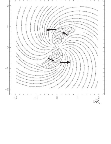
Figure 15: Structure of magnetic field lines in the equatorial plane of an orthogonal rotator $\chi=90^{\circ}$ for nonzero longitudinal currents. The asymmetric form of the closed magnetosphere (hatched region) could lead to an electromagnetic energy flow to the region of open field lines.

We note one more point. Substituting Eqn (62) for the electric field (again for zero potential $\psi$) in the expression for the Poynting vector ${\bf S}(r,\theta,\varphi)=(c/4\pi)[{\bf E}\times{\bf B}]$, we immediately obtain

$${\bf S}=\frac{\Omega r}{4\pi}(-B_{\varphi}\sin\theta\,{\bf B}+B^{2}{\bf e}_{\varphi}).$$ (89)

It might seem that the second term in this equation cannot contribute to the energy losses because it is orthogonal to the normal vector. Consequently, the energy flux should be directed along the magnetic field lines only. However, as shown in Fig. 15, in the nonaxisymmetric case (due to the possible difference in the magnetic field ${\bf B}$ at different boundaries of the closed magnetosphere), this term could be responsible for the total energy flux from the closed magnetosphere into the open field lines region, along which the energy is further transported beyond the light cylinder.

Thus, in the general case, in addition to the current losses discussed in Section 1, the neutron star spin-down can be related to perturbations of the normal magnetic field component $B_{n}$. This additional contribution to the braking torque $K_{\perp}$ can be due to a violation of the exact compensation between the magnetodipole radiation from the central star and magnetosphere radiation that occurs for a zero longitudinal current.

2.3.3 Additional torque: separatrix currents.

To discuss one more possible additional torque, we consider in more detail the spin-down of an orthogonal rotator due to surface currents across polar caps, which corresponds to the first term in expansion (84). For this, it is convenient to rewrite the braking torque in the original form:

$${\bf K}=2\,\int[{\bf r}\times\frac{[{\bf J}_{\rm s}\times{\bf B}]}{c}]\,{\rm d}s.$$ (90)

Hence, the full losses $W_{\rm tot}=-{\bf\Omega}\cdot{\bf K}$ become

$$W_{\rm tot}=2\,\frac{\Omega R}{c}\int J_{\theta}B_{n}{\rm d}s.$$ (91)

From Eqn (90), it can be erroneously concluded [156] that the braking torque for the local Goldreich current $i_{\rm s}^{\rm A}=i_{\rm a}^{\rm A}=1$ should not strongly depend on the inclination angle $\chi$. Indeed, for $\chi\approx 90^{\circ}$ the surface current $J_{\rm s}^{(90)}$ closing the volume currents flowing in the magnetosphere (and, hence, proportional to $\cos\theta_{\rm b}$) can be evaluated as $J_{\rm s}^{(90)}\sim\varepsilon^{1/2}J_{\rm s}^{(0)}$. But the characteristic distance $r_{\perp}=R$ from the axis to the polar cap, conversely, increases in the same proportion; $r_{\perp}^{(90)}\sim\varepsilon^{-1/2}r_{\perp}^{(0)}$.

However, the exact analysis [69] demonstrates that this argument, which is self-evident at first glance, ignores the real structure of the surface currents inside the polar cap. As shown in Fig. 16, the surface currents closing the volume currents should flow in such a way that the surface current $J_{\theta}$ averaged over the surface vanishes (although just this component determines the neutron star energy losses). Therefore, when calculating the energy losses, the higher-order effects in the parameter $\varepsilon=\Omega R/c$ must be taken into account.

Figure 16: Structure of the volume (light arrows), separatrix (dark arrows), and surface (thin lines) currents near the polar cap of an orthogonal rotator. The additional separatrix current is shown by the dashed line.

But if the surface current $<J_{\theta}>$ averaged over the polar cap is zero, then, along the separatrix dividing the region of open and closed field lines, there should be a surface current comparable to the full current flowing in the open field line region, as is shown in Fig. 16. For example, for a circular polar cap and for the local Goldreich current (when the answer can be obtained analytically), the inverse current should be $3/4$ of the volume current [157].

One important note is in order here, however. The above conclusion on the energy losses was based on the assumptions that there are no volume longitudinal currents inside the closed magnetosphere and that the surface currents closing the volume currents exist only inside the polar cap area and do not go beyond it [158]. If we relax these assumptions, the problem of the neutron star spin-down becomes ill-defined because it is impossible to calculate the additional current circulating inside the magnetosphere but not entering the pulsar wind region. Indeed, as shown in Fig. 16, additional separatrix currents must result in a nonzero mean surface current $<J_{\theta}>\neq 0$ across the polar cap and hence in additional energy losses.

Thus, theoretical analysis has not resulted in sufficient clarity here. Some clarification became possible only after numerical modeling of the magnetosphere of an oblique rotator was carried out. As a result, it was shown that there are indeed no volume currents in a closed magnetosphere. It was also remarkable that the inverse currents along the separatrix were also obtained in numerical simulations [159]. But the inverse current was found to amount to only 20% of the volume current. Of course, such a discrepancy could be explained by the fact that the radius of the star was only two to three times as small as the light cylinder in these calculations. However, the significant difference between these parameters could also be related to additional separatrix currents ignored in the previous analysis. The ‘doomed uncertainty’ persisted.

2.3.4 Direct grasp of the truth.

We now return to the discussion of energy losses of a rotating neutron star. We recall that the direct current losses discussed above, Eqns (37) and (38), correspond to only the first term in expansion (84). They are due to the surface currents closing volume currents in the magnetosphere. Therefore, by the way, the action of this braking mechanism is concentrated in the polar cap area only. And the magnetic field corresponds to the zeroth-approximation magnetic field (the dipole magnetic field is close to a uniform field within the polar cap area). As we have seen, the direct current losses cannot explain the energy losses $W_{\rm tot}^{({\rm MHD})}$ in (49) for the ’universal solution’.

On the other hand, as shown in Sections 2.3.2 and 2.3.3, there are two more reasons for the radio pulsar spin-down. First, the example of vacuum losses demonstrates that the second term in expansion (84) should not be ignored in general. In the expression ${\bf J}_{\rm s}\times{\bf B}$ for this term, the surface current ${\bf J}_{\rm s}$ corresponds to the zeroth-approximation current and the magnetic field is related to the rotation-induced third-order perturbation (in this case, the entire surface of the neutron star participates). Another possible reason could be the additional separatrix currents that are closed inside the polar cap area. Clearly, as before, they would correspond to the first term in expansion (84).

As noted above, it was impossible not only to calculate analytically but even to estimate the corresponding contributions. Therefore, it is not surprising that virtually nothing was previously known about these losses. However, we can now answer this question by directly analyzing the numerical results.

But before showing the hand, we write the additional braking torque in the general form as

$$K_{\perp}^{\rm add}=-A\,\frac{B_{0}^{2}\Omega^{3}R^{6}}{c^{3}}\,i_{\rm a}$$ (92)

and try to estimate the dimensionless constant $A$ from the result of numerical modeling of the ‘universal solution’. As shown in Section 1.3, the dimensionless antisymmetric longitudinal current is $i_{\rm a}^{\rm A}\approx(\Omega R/c)^{-1/2}$; therefore, one can evaluate the coefficient $A$ as

$$A\sim(\Omega R/c)^{1/2}.$$ (93)

For such a small $A\ll 1$, we can disregard the additional torque $K_{\perp}^{\rm mag}$ in Eqn (92) for the local Goldreich current $i_{\rm a}^{\rm A}\sim 1$, which was in fact done in the BGI model (see Section 3.1.1).

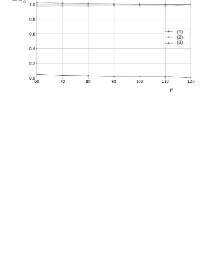
Figure 17: Electromagnetic energy flux $S$ from the closed (bottom curve) and open (middle curve) magnetic field line region for the angle $\chi=60^{\circ}$. The upper curve corresponds to the total power. The neutron star radius (50 units) is 10 times smaller than the light cylinder radius ($\varepsilon=0.1$). $S_{0}$ is the energy flux corresponding to the energy losses $W_{\rm tot}^{({\rm MHD})}$ in Eqn (49).

And here is the correct answer inferred from the processing of the numerical calculation data [160]. Figure 17 shows the electromagnetic energy flux as a function of the radius $r$ for the angle $\chi=60^{\circ}$ from the closed (bottom curve) and open (middle curve) line regions. The sizes of the star and the light cylinder are 50 and 500 units ($\varepsilon=0.1$).

As we see, almost all the energy flux is concentrated in the open magnetic line region. This means that in the numerical simulations reproducing the ‘universal solution’, the energy losses from an oblique rotator are likely to be due to additional separatrix currents. This solution does not reveal any energy flux from the closed magnetosphere, which would otherwise be present. We do not even need to mention that these results leave no room for magnetodipole losses (in that case, the energy flux would also be distributed quite homogeneously and would not be concentrated in the open field line region only).

Now, using Eqn (91), it is possible to obtain the expression for the surface current $<J_{\theta}>$ averaged over the polar cap area that provides the MHD losses $W_{\rm tot}^{({\rm MHD})}$ given by formula (49). In particular, for an orthogonal rotator, we obtain

$$<J_{\theta}>=\frac{c}{4\pi f_{\ast}}\,B_{0}\,\left(\frac{\Omega R}{c}\right)^{2}.$$ (94)

Accordingly, the averaged magnetic field $<B_{\varphi}>$ in the open field line region at a distance $r$ is

$$<B_{\varphi}>=\frac{1}{f_{\ast}}\,B_{0}\,\left(\frac{\Omega R}{c}\right)^{2}\frac{R}{r}.$$ (95)

This can be easily obtained by calculating the electromagnetic energy flux through the corresponding area: $s(r)=f_{\ast}\pi(\Omega/c)^{1/2}r^{3/2}$. As we see, the field $B_{\varphi}$ behaves as if in a magnetodipole wave. The difference is that this radial dependence takes place inside the light cylinder and not only in the wave zone. Finally, we note that the full separatrix current should be $(\Omega R/c)^{1/2}$ times smaller than the full current circulating in the magnetosphere.

2.3.5 Anomalous torque.

To conclude this section, we note another curious point. Besides the torque considered above, which leads to spin-down and the inclination angle $\chi$ evolution of a rotating magnetized ball, there is the so-called anomalous torque directed along the $y^{\prime}$ axis perpendicular to the plane formed by the magnetic moment ${\bf m}$ and the spin axis ${\bf\Omega}$. This torque is called anomalous because of its amplitude,

$$K_{y^{\prime}}=\xi\,\frac{{\bf m}^{2}}{R^{3}}\left(\frac{\Omega R}{c}\right)^{2}\sin\chi\cos\chi,$$ (96)

where $\xi$ is a numerical factor of the order of unity, which is $(\Omega R/c)^{-1}$ times the braking torque components $K_{x^{\prime}}$ and $K_{z}$. Various authors give different values of $\xi$: $\xi=1$ [161, 162], $\xi=3/5$ [163], $\xi=2/5$ [164], $\xi=1/5$ [156, 165], $\xi=0$ [166, 167] (in decreasing order).

Clearly, the situation where no full concordance is achieved on a problem that is elementary at first glance was surprising. We recall that neutron star precession due to the anomalous torque, being superimposed on the secular pulsar spin-down, should change the observed braking index $n_{\rm br}=\ddot{\Omega}\Omega/{\dot{\Omega}}^{2}$ [163, 168, 169]. Thus, this question is of both theoretical and purely practical interest.

The analysis performed in [152] showed that unlike the braking torque considered above, the determination of the anomalous torque requires taking both the electric force ${\bf E}\,\sigma_{n}$ (where $\sigma_{n}$ is the surface charge density) and the angular momentum of the electromagnetic field inside the star into account. As a result, the anomalous torque depends on the internal structure of the magnetic field.

Indeed, in almost all the papers mentioned above, the anomalous torque ${\bf K}$ was calculated as the flux $K_{i}=-\oint\varepsilon_{ijk}r_{j}T_{kl}{\rm d}s_{l}$ of the electromagnetic stress tensor $T_{kl}$ using the formula [65]

$${\bf K}^{M}=\frac{1}{4\pi}\oint\Bigl{(}\left[{\bf r}\times{\bf B}\right]\left({\bf B}\cdot{\rm d}{\bf s}\right)+\left[{\bf r}\times{\bf E}\right]\left({\bf E}\cdot{\rm d}{\bf s}\right)$$

$$-\frac{1}{2}\leavevmode\nobreak\ ({\bf E}^{2}+{\bf B}^{2})\left[{\bf n}\times{\rm d}{\bf s}\right]\Bigr{)}.$$ (97)

Integrating over the sphere yields

$${\bf K}^{M}_{y^{\prime}}=\frac{R}{4\pi}\oint\Bigl{(}\left[{\bf n}\times{\bf B}\right]_{y^{\prime}}\left({\bf B}\cdot{\bf n}\right)+\left[{\bf n}\times{\bf E}\right]_{y^{\prime}}\left({\bf E}\cdot{\bf n}\right)\Bigr{)}{\rm d}s.$$ (98)

However, the correct derivation of the electromagnetic torque for a ball requires caution. Indeed, using general relation (81) and expressing the surface charges and currents through the corresponding jumps $\{{\bf E}\}$ and $\{{\bf B}\}$ in the electric and magnetic fields, we obtain the total torque in the form

$${\bf K}=\int{\bf r}\times{\rm d}{\bf F}$$ (99)

$$=\frac{R}{4\pi}\oint\Bigl{(}\left[{\bf n}\times\left\{{\bf B}\right\}\right]\left({\bf B}\cdot{\bf n}\right)+\left[{\bf n}\times{\bf E}\right]\left(\left\{{\bf E}\right\}\cdot{\bf n}\right)\Bigr{)}{\rm d}s.$$

This formula differs from (98) in having the electric and magnetic field jumps on the surface of the ball, which exactly determine the surface charges and currents. As shown in [152], exactly this expression should be used when determining the torque for a rotating magnetized ball.

The point is that the angular momentum vector flux of the electromagnetic field is related to the angular momentum of forces acting on matter via the angular momentum conservation law for the electromagnetic field, which has the form

$$\frac{{\rm d}\,{\bf L}_{\rm field}}{{\rm d}t}+\int[{\bf r}\times{\bf F}]{\rm d}V={\bf K}^{M},$$ (100)

where

$${\bf L}_{\rm field}=\int\frac{[{\bf r}\times[{\bf E}\times{\bf B}]]}{4\pi c}{\rm d}V$$ (101)

is the angular momentum of the electromagnetic field in a volume $V$, ${\bf K}^{M}$ is the angular momentum flux of the field through the surface bounding this volume, and ${\bf F}=\rho_{\rm e}{\bf E}+[{\bf j}\times{\bf B}]/c$ is the Lorentz force density. The last term in Eqn (100) plays the role of the source or sink and is therefore responsible for the transfer of the electromagnetic field angular momentum to matter,

$$\frac{{\rm d\,{\bf L}_{\rm mat}}}{{\rm d}t}=\int[{\bf r}\times{\bf F}]{\rm d}V.$$ (102)

It is this term, and not ${\bf K}^{M}$, as most of the papers assumed, that has the meaning of the torque applied to a rotating body. Therefore, to calculate the anomalous torque (in the second order in the parameters $\varepsilon=\Omega R/c$), we should indeed take the angular momentum of the electromagnetic field into account. Some of the stresses related to the electromagnetic field should affect the angular momentum of the field itself, and some others should affect the interaction with the rotating body. According to Eqn (100), this means that for the angular momentum of forces applied to the ball, we should use the formula

$${\bf K}\equiv\frac{{\rm d}{\bf L}_{\rm mat}}{{\rm d}t}={\bf K}^{M}-\frac{{\rm d}\,{\bf L}_{\rm field}}{{\rm d}t}.$$ (103)

The correct expression for ${\bf K}^{M}$ (independent of the internal structure of the field!) was first derived by Melatos [163]:

$$K_{y^{\prime}}^{M}=\frac{3}{5}\,\frac{{\bf m}^{2}}{R^{3}}\left(\frac{\Omega R}{c}\right)^{2}\sin\chi\cos\chi.$$ (104)

The quantity ${\rm d}\,{\bf L}_{\rm field}/{\rm d}t$, turned out, as was already mentioned, to be dependent on the internal structure of the star.

As a result, the anomalous torque applied to a homogeneously magnetized ball was found to be [152]

$${K}_{y^{\prime}}=\frac{1}{3}\,\frac{{\bf m}^{2}}{R^{3}}\left(\frac{\Omega R}{c}\right)^{2}\sin\chi\cos\chi.$$ (105)

On the other hand, for a rotating hollow sphere, when charges and currents are concentrated inside the spherical shell $r=R$, we obtain

$${K}_{y^{\prime}}=\frac{31}{45}\,\frac{{\bf m}^{2}}{R^{3}}\left(\frac{\Omega R}{c}\right)^{2}\sin\chi\cos\chi.$$ (106)

Finally, if the homogeneous magnetic field is present only inside the inner radius $R_{\rm in}$, and for $R_{\rm in}<r<R$ (also outside the ball) the zeroth-order magnetic field is identical to that of a point-like dipole, we have

$${K}_{y^{\prime}}=\left(\frac{8}{15}-\frac{1}{5}\frac{R}{R_{\rm in}}\right)\frac{{\bf m}^{2}}{R^{3}}\left(\frac{\Omega R}{c}\right)^{2}\sin\chi\cos\chi.$$ (107)

For $R_{\rm in}=R$, we return to the previous value $\xi=1/3$.

As regards the spin-down of the ball (i.e., the third-order effect in the parameter $\varepsilon$), the angular momentum of the electromagnetic field was found to be insignificant in this case. Therefore, formula (83) for the torque applied to a rotating ball is valid and independent of the internal structure of the field.

3 BGI theory thirty years later

We take this opportunity to present a detailed analysis of the theory of magnetospheres and radio emission of pulsars formulated in the 1980s in a series of papers [67, 170-172] and later collected in monograph [69]; several significant improvements were added later in [151, 173-177].

3.1 Theory of the pulsar magnetosphere

3.1.1 Basics.

The main results of the BGI theory on the magnetosphere structure can be formulated as follows.

• The longitudinal current $j_{\parallel}$, outflowing from magnetic poles (more precisely, its symmetric part $j_{\rm s}$), does not exceed the local Goldreich current $j_{\rm GJ}\approx\Omega B_{0}\cos\chi/2\pi$.

• The amplitude of the local current is determined by the drop in the electric potential $\psi$; the dimensionless symmetric current amplitude $i_{\rm s}^{\rm A}$ is

  $$i_{\rm s}^{\rm A}(\Omega,B_{0},\chi)\approx\frac{1}{2}\left(\frac{\psi}{\psi_{\rm max}}\right)^{1/2},$$ (108)

  where, again, $\psi_{\rm max}$ is the maximum potential difference (23).

• The potential $\psi$ is given by the Ruderman-Sutherland model $\psi_{\rm RS}$, Eqn (21).

• The dependence of the inclination angle $\chi$ on both the maximum potential drop $\psi_{\rm max}=\psi_{\rm max}(0)\cos\chi$ and the potential $\psi_{\rm RS}$ is taken into account; the analysis of the evolution of radio pulsars takes the dependence on the angle $\chi$ and on the location of the ‘death line’ into account.

• Due to the relatively small value of the longitudinal current, there is a light surface beyond the light cylinder (see Fig. 7) at which the outflowing plasma is accelerated up to energies $\sigma_{\rm M}m_{\rm e}c^{2}$.

As a result, the key parameter in the BGI theory is the dimensionless quantity $Q\approx i_{\rm s}$, which can be represented in the form [170]

$$Q=2\,P^{11/10}{\dot{P}}_{-15}^{-2/5},$$ (109)

or more precisely, in terms of the angle $\chi$

$$Q=P^{15/14}B^{-4/7}_{12}\cos^{2d-2}\chi,$$ (110)

where $d\approx 0,75$. The condition $Q=1$ for Eqn (110) exactly corresponds to the relation $\psi_{\rm max}(\chi)=\psi_{\rm RS}(\chi)$ defining the ’death line’. Therefore, in pulsars for which definition (109) gives $Q>1$, it is possible to expect an irregular generation of the secondary electron-positron plasma and hence a decreased value of $\dot{P}$, which results in the observed values $Q>1$. Thus, for these pulsars, we should set $Q=1$. The parameter $Q$ is convenient because it determines some key characteristics, such as the total energy losses:

$$W_{\rm tot}^{({\rm BGI})}\approx Q\frac{B_{0}^{2}\Omega^{4}R^{6}}{c^{3}}\cos^{2}\chi,$$ (111)

and the energy flux carried by particles inside the light cylinder,

$$W_{\rm tot}^{\rm out}\sim Q^{2}\,W_{\rm tot}.$$ (112)

The last equation coincides with the total particle flux toward the neutron star surface in the inner gap:

$$W_{\rm part}^{\rm in}\sim Q^{2}W_{\rm tot}.$$ (113)

We keep in mind, finally, that the angle $\chi$ tends to 90^∘ in this model: $\Omega\sin\chi={\rm const}$.

3.1.2 Magnetosphere structure.

One of the features that distinguish the BGI theory from numerical results obtained in recent years lies in the assumption that the longitudinal current flowing in the open line region is determined by the magnetosphere structure inside the line cylinder and not beyond it. It is the matching of solutions in the closed and open parts of the magnetosphere that determined the ‘Ohm law’ $i_{\rm s}\propto\psi_{\rm RS}^{1/2}$ given by formula (108) underlying the theory [67]. It was also shown that the minimal energy corresponds to a solution in which the null point lies on the light cylinder and not at shorter distances from the neutron star [178].

Here, however, we assumed that the longitudinal current $i_{\parallel}$ (except in the orthogonal rotator case, of course) remains almost constant everywhere within the open line region and does not change sign near the separatrix, as the ‘universal solution’ now requires. This, in particular, has led to a different topology of the magnetic surfaces at the crossing of the equator with the light cylinder (an X, but not a Y point). However (and we wish to especially stress this here), a much more significant difference between the BGI theory and the ‘universal solution’ considered at present was the existence of the light surface changing the entire structure of the flow beyond the light cylinder.

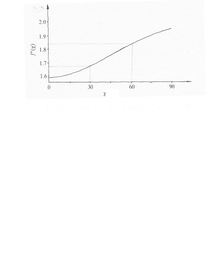
Figure 18: Dimensionless polar cap area $f_{\ast}(\chi)$ as a function of the angle $\chi$ [91]. It coincides up to 10% with the numerical modeling in [112].

Nevertheless, the analytic solutions obtained more than thirty years ago for an oblique rotator in the BGI theory proved to be surprisingly close in many respects to the characteristics obtained for the ‘universal solution’. For example, the form of the closed magnetosphere shown in Figure 4 almost coincides with the result presented in Fig. 10. Moreover, the dependence of the dimensionless polar cap area $f_{\ast}(\chi)$ on the angle $\chi$ (Fig. 18) found in monograph [91] coincides up to 10% with the dependence $f_{\ast}(\chi)\approx(1+0.2\,\sin^{2}\chi)f_{\ast}(0)$ derived quite recently in [112]. This means that the longitudinal currents in the magnetosphere do not strongly disturb the closed field line region.

As regards the prediction of an effective acceleration of outflowing plasma near the light surface, this conclusion, as stressed above, has not been confirmed so far by numerical calculations. However, as noted in Section 1.7, a need for particle creation beyond the light cylinder is being widely discussed at present. Moreover, it is often claimed that beyond the light cylinder, there are regions where the electric field exceeds the magnetic field. However, here, one usually means a current sheet and not the light surface that is shown in Fig. 7. The existence of the light surface $|{\bf E}|=|{\bf B}|$ near the light cylinder was also mentioned in [179]. However, the ‘Aristotle’ approach discussed in this paper in fact limits the values of the longitudinal current from above, which actually leads to diminishing the toroidal magnetic field.

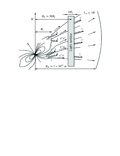
Figure 19: Light surface near the light cylinder proposed in [180] to explain the observed variability of the Crab Nebula pulsar at TeV energies.

Nevertheless, we would like to draw attention to the paper by Aharonian, Bogovalov, and Khangulyan [180], in which, in our opinion, direct observational clues of the effective particle acceleration on light surfaces were found. By the way, this paper is entitled ‘’Abrupt acceleration of a ‘cold’ ultrarelativistic wind from the Crab pulsar”. As shown in Fig. 19, this model is geometrically surprisingly similar to our model (see Fig. 7). In particular, it is shown in [180] that the observed variability at TeV energies [181] can be explained if, at distances of the order of $30\,R_{\rm L}$ from the neutron star, acceleration of particles to energies corresponding to the Lorentz factor $\gamma\approx 10^{6}$ occurs. As noted above, the value $\gamma\sim 10^{6}$ exactly corresponds to estimate (19) of the magnetization parameter $\sigma_{\rm M}$ of the pulsar magnetosphere in the Crab Nebula. Last, the scale $30\,R_{\rm L}$ is definitely smaller than the fast magnetosonic surface distance $r_{\rm F}\approx 100\,R_{\rm L}$, and therefore the particle acceleration process based on the force-free solution considered in [62, 182] can be applied here.

3.1.3 Braking index.

Table 1: Braking index $n_{\rm br}={\ddot{\Omega}}\Omega/{\dot{\Omega}}^{2}$ for fast pulsars [186].

PSR	J1734+3333	B0833$-$45	J1833$-$1034	B0540$-$69	B0531+21	B1509$-$59	J1640$-$4631
		Vela			Crab
$n_{\rm br}$	0.9(2)	1.4(2)	1.857(1)	2.14(1)	2.51(1)	2.839(1)	3.15(3)

As is well known, direct information on the spin-down mechanism should be obtained from the value of the so-called ‘braking index’ [183, 184]

$$n_{\rm br}=\frac{{\ddot{\Omega}}\Omega}{{\dot{\Omega}}^{2}}.$$ (114)

However, as is also well known, this parameter cannot be directly used to analyze the radio pulsar evolution, unfortunately: the regular pulsar spin-down is superimposed with additional fluctuations on time scales much shorter than the dynamical age of pulsars $\tau_{\rm D}\sim P/{\dot{P}}$. This results in ${\ddot{\Omega}}$ being not indicative of the secular pulsar spin-down. As already noted in Section 2.3.5, such perturbations can most likely be related to the neutron star precession due to its nonspherical shape (see, e.g., [163, 169]). For this reason, measurements of most of the pulsars give $n_{\rm br}=\pm(10^{4}$–$10^{5})$[169], which does not relate to the secular pulsar spin-down mechanism. As a result, only braking indices of a handful of young pulsars can be used to analyze the energy loss mechanism; for other radio pulsars, longer observations are needed to measure the average braking index.

Table 1 shows that observations of most of the young pulsars yield $n_{\rm br}\sim 3$, which, in the zeroth approximation, does not contradict any of the pulsar spin-down theories:

$$n_{\rm br}^{({\rm V)}} = 3+2\,{\rm ctg}^{2}\chi,$$ (115)

$$n_{\rm br}^{({\rm BGI})} \approx 1,93+1,5\,{\rm tg}^{2}\chi,$$ (116)

$$n_{\rm br}^{({\rm MHD})} \approx 3+2\frac{\sin^{2}\chi\,\cos^{2}\chi}{(1+\sin^{2}\chi)^{2}}.$$ (117)

On the other hand, to infer the evolution law from observations, it is necessary, as we have seen, to measure the braking index $n_{\rm br}$ with a precision of two significant digits by segregating this quantity from the background of much larger fluctuations. Presently this cannot be done, unfortunately. Nevertheless, we note that for most young pulsars, $n_{\rm br}<3$. As we see again, there is good correspondence with the BGI theory predictions. As regards the ‘universal model’, for which $3<n_{\rm br}^{({\rm MHD})}<3.25$, it was shown in [185] that the account for the additional precession enables bringing this theory into accordance with observations as well.

3.1.4 Evolution of the inclination angle.

Of course, the spin-down theory could be tested by measurements of the angle $\chi$ evolution, i.e., by the sign of the time derivative $\dot{\chi}$. Unfortunately, so far there are no reliable estimates of this quantity (see, however, [187]). This is mainly due to the lack of a quantitative theory of radio emission from pulsars, which does not allow connecting the secular changes in the mean pulse profiles with the angle between the magnetic and rotation axes.

Nevertheless, it can not be said that there are no result devoted to the analysis of the evolution of the inclination angle $\chi$. In particular, the Crab pulsar observations carried out over several decades reported in recent paper [187] might favor the counter-alignment (the angle $\chi$ tending to $90^{\circ}$). However, this paper made several model assumptions (for example, that the gamma-ray pulse profile changed with time in the same way as in the radio range), which precludes us from considering this evidence as final.

Many attempts have also been made to infer the angle $\chi$ evolution from analysis of the pulsar distributions over $\chi$ itself and the mean pulse profile widths [189-194]. Here, alignment (the angle $\chi$ tending to zero) was frequently obtained. However, as has been noted many times (see, e.g., [151]), the dependence of the ‘death line’ on the angle $\chi$ has been ignored. As shown in Fig. 14, for sufficiently large periods $P$, plasma generation is possible only for small $\chi$. Hence, irrespective of the evolution of individual pulsars, the mean value of the inclination angle $<\chi>$ should decrease with the spin period.

Clearly, fully taking the ‘death line’ dependence on the angle $\chi$ into account can be done using only the kinetic approach, in which two-parameter (multi-parameter) distributions are analyzed. Unfortunately, up to now most studies have ignored the $\chi$ angle evolution [195-199]. Only recently have papers appeared where it was systematically taken into account [200-203]. However, these studies have not made definitive conclusions about the direction of the inclination angle evolution either.

Our recent paper [177] also failed to answer this question. In that paper, we attempted to formulate a test to determine the $\chi$ angle evolution direction. The idea, as was already mentioned above, was to use the analysis of the fraction of interpulse pulsars, i.e., pulsars that show, besides the main pulse, another emission pulse located roughly in the middle between consecutive main pulses (i.e., at the phase $\phi\approx 180^{\circ}$).

As shown in Fig. 14, the interpulse can be observed in pulsars either with $\chi\approx 90^{\circ}$ (when the interpulse is due to emission from another magnetic pole) or with $\chi\approx 0^{\circ}$ (when the main pulse and the interpulse are due to crossing by the line of sight of ‘hollow cone’ radio emission). Clearly, the number of pulsars with $\chi\sim 0^{\circ}$ and $\chi\sim 90^{\circ}$ depends significantly on the $\chi$ angle evolution direction. However, it turned out that the observed number of interpulse pulsars can be explained by both the BGI model (counter-alignment) and the MHD model (alignment). This is due to a large uncertainty in the initial pulsar distribution over the angle $\chi$ and the spin period $P$. In any case, the observed angle $\chi$ distribution was shown to be consistent with the BGI model.

3.1.5 Surface heating.

To conclude this section, we return to the problem of neutron star heating by the inverse particle flux $W_{\rm part}^{\rm in}$ in the plasma generation region. According to (113), in the BGI model, the energy of these particles should be $Q^{2}$ times smaller than the total energy losses $W_{\rm tot}$. Therefore, we can expect that the X-ray luminosity $L_{\rm X}$ would also depend in a similar way on the total energy losses of the pulsar.

Figure 20 shows the ratio $L_{\rm X}/W_{\rm tot}$ as a function of parameter $Q$ in Eqn (109). The thermal X-ray luminosity $L_{\rm X}$ of the polar caps was taken from [140-142]; the errors are related to both uncertainty in the pulsar distances (pulsars PSR J0205+6449 and J2021+3651) and the flaring activity (PSR J1119-6127 and J1846-0258) unrelated to the polar cap heating. The line corresponds to the $Q^{2}$ law. As we see, within the measurement errors, the X-ray luminosity from the polar cap thermal heating does not contradict theoretical predictions.

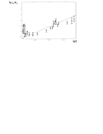
Figure 20: Ratio $L_{\rm X}/W_{\rm tot}$ as a function of the parameter $Q$. Thermal luminosities of the polar caps $L_{\rm X}$ are taken from [140-142]; the line corresponds to the $Q^{2}$ dependence.

3.2 Theory of radio emission

3.2.1 Basic.

The principal statements of the BGI theory about pulsar radio emission can be formulated as follows [69, 172].

• The main instability determining the observed coherent radio emission is the curvature plasma instability of ‘mode 4’ (Fig. 21).

• A saturation of the instability is due to three-wave decay of ‘mode 4’ into extraordinary (’mode 1’, or X-mode) and ordinary (’mode 2’, or O-mode) waves capable of leaving the neutron star magnetosphere.

• The ordinary wave propagates with deviation from the magnetic axis and forms the outer (conal) radio beam, whereas the extraordinary wave propagates along a straight line and forms the inner (core) beam component.

• The total radio luminosity makes up the fraction a $\alpha=10^{-4}$–$10^{-5}$ of the particle energy flux ejected from the neutron star magnetosphere.

• The radio emission has a power-law spectrum with the spectral index ranging from $-1$ to $-3$; at the frequency $\nu_{\rm max}\approx 3\,P^{-1/2}\,\Gamma_{100}^{7/4}$ GHz, there is a spectral break with the change in the spectral index by approximately 1, and a low-frequency ‘cut-off’ occurs at the frequency

  $$\nu_{\rm min}\approx 120\,P^{-1/2}\Gamma_{100}^{-3/4}B_{12}^{1/2}\,{\rm MHz}.$$ (118)

  Here, $\Gamma\approx<\gamma>$ is the characteristic Lorentz factor of the plasma and $\Gamma_{100}=\Gamma/100$.

Below, we formulate the main properties of these modes in more detail, discuss theoretical predictions, and compare them with observations.

3.2.2 Mode classification.

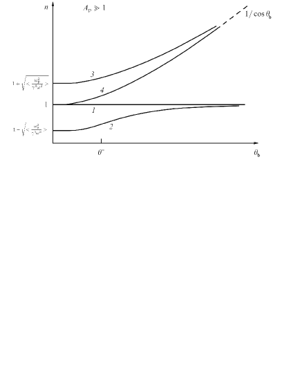
Figure 21: Normal modes with the refractive indices $n\approx 1$ propagating from the neutron star surface as a function of the angle $\theta_{\rm b}$ between the wave vector ${\bf k}$ and the external magnetic field ${\bf B}$. Waves 1 (extraordinary X-mode) and 2 (ordinary O-mode) can escape from the pulsar magnetosphere.

The radio waves propagating in pulsar magnetospheres can be easily classified by analyzing the dielectric permittivity tensor in the limit of the infinite magnetic field when particles can move only along magnetic field lines:

$$\varepsilon_{ij}(\omega,{\bf k})=\begin{bmatrix}1&0&0\\ 0&1&0\\ 0&0&1-<\dfrac{\omega_{\rm pe}^{2}}{\gamma^{3}(\omega-{\bf kv})^{2}}>\end{bmatrix}.$$ (119)

Here, $\omega_{\rm pe}=(4\pi e^{2}n_{\rm e}/m_{\rm e})^{1/2}$ is the nonrelativistic electron plasma frequency and the angular brackets denote averaging over a distribution function. It turns out that this simple model allows discovering quite unusual properties. Indeed, we consider the limit case

$$A_{\rm p}=\frac{\omega_{\rm pe}^{2}}{\omega^{2}}\,\Gamma\gg 1,$$ (120)

realized at sufficiently small distances from the neutron star, $r<r_{\rm A}$, where [69]

$$r_{\rm A}\approx 10^{2}R\cdot\lambda_{4}^{1/3}\Gamma_{100}^{1/3}B_{12}^{1/3}\nu_{\mathrm{GHz}}^{-2/3}P^{-1/3}.$$ (121)

In this parameter region, the solution of the corresponding dispersion equation yields the following four normal modes at small angles $\theta_{\rm b}$ between the wave vector ${\bf k}$ and the external magnetic field ${\bf B}$ (see Fig. 21):

$$n_{1} = 1,$$ (122)

$$n_{2} \approx 1+\frac{\theta_{\rm b}^{2}}{4}-\left(<\frac{\omega_{\rm pe}^{2}}{\gamma^{3}\omega^{2}}>+\frac{\theta_{\rm b}^{4}}{16}\right)^{1/2},$$ (123)

$$n_{3} \approx 1+\frac{\theta_{\rm b}^{2}}{4}+\left(<\frac{\omega_{\rm pe}^{2}}{\gamma^{3}\omega^{2}}>+\frac{\theta_{\rm b}^{4}}{16}\right)^{1/2},$$ (124)

$$n_{4} \approx 1+\frac{\theta_{\rm b}^{2}}{2}.$$ (125)

We note that in [204], where such waves were first investigated, ’mode 2’ was omitted. There, ‘mode 4’ was called an ‘ordinary’ wave, which in fact corresponds to the ordinary wave at small angles $\theta_{\rm b}$. Subsequently, in many papers studying the theory of radio emission, only three types of radio waves were considered [205-207].

However, as we see, when the condition $A_{\rm p}\gg 1$ is satisfied (see (120)) for large angles $\theta_{\rm b}>\theta^{\ast}$, where

$$\theta^{\ast}=\left(<\frac{\omega_{\rm pe}^{2}}{\gamma^{3}\omega^{2}}>\right)^{1/4},$$ (126)

the dispersion curve of ‘mode 4’ is close to that of a relativistic Alfvén wave with the refractive index $n\approx 1/\cos\theta_{\rm b}$, and this means that at large angles $\theta_{\rm b}$ ‘mode 4’ propagates along the magnetic field lines and cannot leave the neutron star magnetosphere (as correctly stated in many papers). Therefore, it is natural to refer to ‘mode 4’ and not ‘mode 2’ as ordinary. For small angles $\theta_{\rm b}$, ‘mode 2’ is a longitudinal plasma wave propagating toward the neutron star in the plasma rest frame; in the laboratory frame, of course, it moves in the opposite direction. For large angles $\theta_{\rm b}$, it transforms into a transverse wave with $n_{2}\approx 1$. It is exactly the difference between $n_{2}$ and unity at small angles $\theta_{\rm b}<\theta^{\ast}$ that leads to the ordinary wave deviating from the magnetic axis. Only very recently was the status of ‘mode 2’ as being ordinary finally recognized [15, 208].

We also note that the theory of polarized emission propagation that we developed in the last few years [175, 209] allows us to determine which of the modes, ordinary or extraordinary, forms the mean radio pulse profile. As was shown in [175, 209], the same signs of the circular polarization (Stokes parameter V) and the derivative ${\rm d}p.a./{\rm d}\phi$ (the rate of change of the position angle of the linear polarization $p.a.$ with the pulse phase $\phi$) correspond to the X-mode, and different signs of these quantities to the O-mode. Lack of space prevents us from discussing this in greater detail.

3.2.3 Radio luminosity as a function of spin period.

In the BGI theory, as noted in Section 3.2.1, the radio luminosity $L_{\rm rad}$ amounts to a fraction $\alpha\sim 10^{-4}$–$10^{-5}$ of the total particle energy flux. On the other hand, by Eqn (112), the energy carried by the particles for sufficiently fast pulsars (i.e., those with $Q<1$) is $Q^{2}$ times the full energy losses $W_{\rm tot}=-J_{\rm r}\Omega\dot{\Omega}$. Therefore, the ratio $L_{\rm rad}/W_{\rm tot}$ for pulsars with $Q<1$ must scale as $\alpha\,Q^{2}$. As shown in Fig. 22, such a dependence is indeed observed (see also [210]). Here, both the slope of the curve (the power-law exponent $2.1\pm 0.1$) and the transformation coefficient $\alpha^{\rm obs}=(2.0\pm 0.2)\times 10^{-5}$ are consistent with the theory with good accuracy.

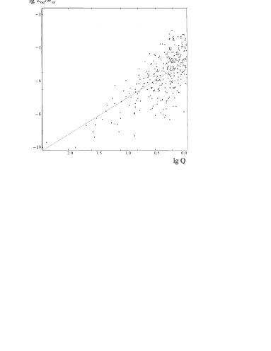
Figure 22: Ratio $L_{\rm rad}/W_{\rm tot}$ as a function of $Q$ in Eqn (110) for radio pulsars with $Q<1$. The data are from the ATNF catalogue [212]; the line corresponds to the dependence $(2.0\pm 0.2)\times 10^{-5}\,Q^{2.1\pm 0.1}$.

Incidentally, using the explicit expression (109) for $Q$, we can find

$$L_{\rm rad}\propto P^{-0.8}{\dot{P}}_{-15}^{0.2}.$$ (127)

The dependence $L_{\rm rad}\propto P^{p}{\dot{P}}^{q}$ has been analyzed many times. E.g., the authors of [211], based on data for 242 pulsars, derived $p=-0.86\pm 0.20$ and $q=0.38\pm 0.08$. In [213], $p=-0.8\pm 0.2$ was obtained. Clearly, these values are consistent with (127). As regards the values $p=-1.39\pm 0.09$ and $q=0.48\pm 0.04$ obtained in [214], the difference can be related to the analysis of all pulsars and not a subset with $Q<1$.

3.2.4 Pulse width a frequency dependence.

As mentioned above, the main difference between two orthogonal modes capable of leaving the neutron star magnetosphere is that the ordinary wave, unlike the extraordinary one, deviates from the magnetic axis. However, according to (121), this can occur only at sufficiently short distances $r<r_{\rm A}$ from the neutron star, at which the condition $A_{\rm p}>1$ is satisfied in accordance with (120). As we see, the region $r<r_{\rm A}$ overlaps with the radio emission generation region, and therefore the ordinary wave refraction should be taken into account in the analysis of the mean radio pulse profiles. We note that in spite of a vast literature devoted to ordinary wave refraction in the neutron star magnetosphere [204, 215-218], in the ‘hollow cone’ model the propagation effects have hardly been taken into account to date.

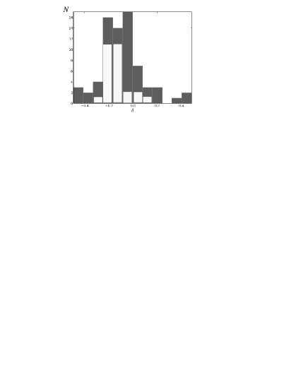
Figure 23: Distribution of pulsars over the exponent $\delta$ [219] determining the dependence of the mean profile width on the frequency $W_{\rm r}\propto\nu^{\delta}$. The isolated part corresponds to pulsars in which the mean pulse is formed by an ordinary wave according to the method described in [175].

Of course, the beam width $W_{\rm r}$ depends not only on the propagation effects but also on the radiation generation level $r_{\rm rad}$. The BGI model (which consistently takes the propagation effects into account) suggested that the radiation at a given frequency $r_{\rm rad}$ can be generated in a wide region up to the distance [172]

$$r_{\rm rad}\sim 3.5\,R\,\nu_{\rm GHz}^{-1}P^{-0.5}\Gamma_{100}^{1.75},$$ (128)

depending, obviously, on the wavelength. As a result, the following expressions for the beam width $W_{\rm r}$ of two normal modes were obtained (here, we omit the weak dependence on the multiplicity $\lambda$, the magnetic field $B_{0}$, and the characteristic Lorentz factor $\Gamma$ of the outflowing plasma):

$$W_{\rm r}^{\rm O} \approx 7.8^{\circ}P^{-0.43}\nu_{\rm GHz}^{-0.14},$$ (129)

$$W_{\rm r}^{\rm O} \approx 10.8^{\circ}P^{-0.5}\nu_{\rm GHz}^{-0.29},$$ (130)

$$W_{\rm r}^{\rm X} \approx 3.6^{\circ}P^{-0.5}\nu_{\rm GHz}^{-0.5}.$$ (131)

The two expressions for the beam width of the ordinary wave correspond to two cases where the main contribution is made by the most and least distant regions from the neutron star. The accuracy of the BGI theory, in which, we recall, the radio emission generation is due to the three-wave decay of ‘mode 4’, did not allow us to answer this question.

Thus, the BGI theory predicts a power-law dependence of the mean radio pulse profile, $W_{\rm r}(\nu)\propto\nu^{\delta}$, with the power-law exponents $\delta=-0.14$ and $\delta=-0.29$ for the ordinary and $\delta=-0.5$ for the extraordinary waves. Figure 23 shows the pulsar distribution over $\delta$ obtained quite recently by the new LOFAR radio telescope [219]. The isolated part corresponds to pulsars in which, according to the method described in our paper [175], the mean pulse is formed by an ordinary wave. It is seen that the pulsar distribution indeed has a sharp maximum at $\delta\approx-0.2$. On the other hand, for pulsar PSR B0943+10, in which the radio emission, according to our method, is formed by an extraordinary wave, the value $\delta\approx-0.5$ was obtained in [220]. Obviously, the BGI theory predictions are consistent with observations here as well.

3.2.5 Low-frequency cut-off.

As we have seen, the accuracy of the determination of spectral indices in the BGI model (which are expected to fall within the range from $-1$ to $-3$) is insufficient to carry out a detailed comparison between the theory and observations. However, no precise measurements have been obtained from observations; these indices are found to be indeed distributed in a wide range (see, e.g., [220]).

By contrast, the low-frequency cut-off at $\nu_{\rm min}$ given by formula (118) is well defined and can be used to compare theory with observations. We note that in the BGI theory, the low-frequency cut-off is due to the very existence of the ordinary wave with the refractive index $n_{2}$ given by formula (123): at frequencies $\nu<\nu_{\rm min}$ [see (118)], this wave cannot escape the neutron star magnetosphere anymore.

Figure 24 presents a comparison between the theory and observations taken from two recent reviews [220, 221]. The line corresponds to the BGI prediction in Eqn (118). Apparently, here again, there is sufficiently good agreement.

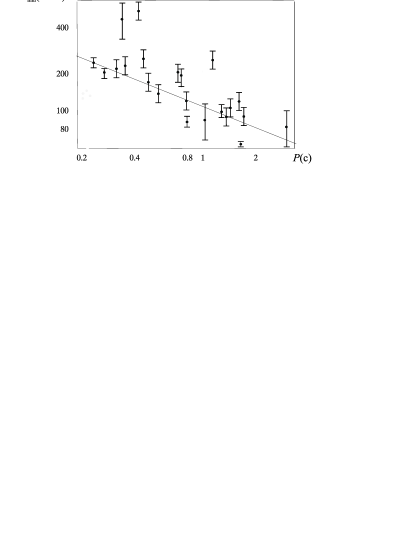
Figure 24: Low-frequency cut-off $\nu_{\rm min}$ as a function of the period $P$. The data are from reviews [220, 221]. The line shows the prediction in Eqn (118).

3.2.6 Statistics of O- and X-modes.

Finally, recent paper [222] enabled theoretical predictions about the O- and X-mode statistics to be tested using a sufficiently large number of data. This paper presents the most complete catalogue to date of polarization properties of 600 radio pulsars at a frequency of 1.4 GHz. In 170 cases the polarization angle of the linear polarization, $p.a.$, and circular polarization (Stokes parameter V) were reliably determined, which allowed finding which of the polarization modes forms the mean radio pulse profile. It was found that in 100 pulsars the mean profile is formed by the X-mode (the same signs of V and ${\rm d}p.a./{\rm d}\phi$), and in 70 pulsars, by the O-mode (different signs of these quantities). Here, as was predicted in [175], most of the X-mode pulsars (86 out of 100) exhibited single-humped mean profiles, and most of the O-mode pulsars (48 out of 70) had double-humped profiles. Both the X- and O-mode pulsars had widths of double-humped profiles a factor of one and a half larger than single-humped ones. This should be the case, because in both cases double-humped and single-humped profiles correspond to the respective central and peripheral crossing of the emission beam.

Figure 25: Distribution of 170 O- and X-pulsars over $W_{\rm r}P^{1/2}$ (in degrees) taken from [222]. The distribution maxima exactly correspond to predictions (129)-(131).

Moreover, the present statistics are sufficient to reliably argue that predictions (129)-(131) about the mean profile width $W_{\rm r}$ for these two modes are also in remarkable agreement with observations. Figure 25 shows distributions of O- and X-pulsars over the quantity $W_{\rm r}P^{1/2}$. Clearly, these histograms are indeed significantly shifted relative to each other, with the distribution maxima being consistent with predictions (129)-(131). As regards the sources with large values of $W_{\rm r}P^{1/2}$, they can easily be explained by widening due to the nonorthogonality of rotators (the observed pulse width is $W_{\rm r}^{\rm obs}=W_{\rm r}/\sin\chi$). As shown in [177], for large $W_{\rm r}^{\rm obs}$, the differential distribution should have the form $N(W_{\rm r}^{\rm obs})\propto(W_{\rm r}^{\rm obs})^{-3}$.

4 Conclusion

The 50 years since the discovery of radio pulsars that have passed smoothly, leave a sense of distinct incompletion. Undoubtedly, much work should be done to understand even the general picture of the physical processes occurring in neutron star magnetospheres. Unfortunately, pulsars do not provide us with clear experiments, and quantitative predictions are frequently difficult to check with observations, as is the case, for example, with the evolution of the inclination angle ${\dot{\chi}}$ or with the mean braking index $n_{\rm br}$.

We note that Physics-Uspekhi has always quickly responded to all important events related to radio pulsar physics. As early as 1969, the first results of the national observations of pulsars both in the radio (Pushchino) [223-225] and in the optical (Crimean Astrophysical Observatory) [226, 227] ranges were published. In the same years, papers by the patriarchs of Russian (Soviet) astrophysicists Shklovskii [228, 229], Ginzburg [230-232], and Zel’dovich [233] were published without delay; for the first time, they performed a serious analysis of physical processes in neutron star magnetospheres. The possibility of pulsar observations in different electromagnetic ranges were discussed in [234-236].

In later years, Physics-Uspekhi published papers devoted to both observations [237-240] and the theory of radio pulsar emission [241-243]. Reviews and conference reports were published about the internal structure of neutron stars [138, 139, 244-249], their evolution [152, 250], and general relativity effects [254-258]. In addition, it should be remembered that B B Kadomtsev, the editor-in-chief of Physics-Uspekhi for many years, wrote the book ‘On the Pulsar’ [259].

Anyway, at present, the theory of pulsar magnetospheres and pulsar wind is a rapidly developing field in which dozens of researchers are working. Substantial progress has been achieved, including some quantitative predictions (for example, formulas for the total energy loss), which, we hope, will be directly tested in the nearest future.

As regards our theory, it has not been much in demand to date, although, as shown above, many statements made more than thirty years ago are at least consistent with observations. However, as mentioned above, direct tests that could shed light on energy release and coherent radio emission mechanisms are not being carried out at present.

In conclusion, the author thanks D Barsukov, A Beloborodov, Ya N Istomin, O Kargaltsev, G Pavlov, A Potekhin, and especially A Philippov for the fruitful discussions of topics in this review. The author would also like to acknowledge A Jessner and J Pétri, who carefully read the text of my popular lecture at the Gamma-2016 conference (Heidelberg, Germany) devoted to similar topics, which enabled me to make several important improvements, and also L Arzamasskiy, A Galishnikova, E Novoselov, and M Rashkovetskiy for help in the calculations. The author separately acknowledges the referee for numerous remarks that greatly improved the style of the paper.

This study was supported by the Russian Foundation for Basic Research grant 17-02-00788.

5 Appendix

Following [36] (see also [50]), we recall how accounting for the toroidal magnetic field time dependence inside the inner gap can influence the plasma generation dynamics. In contrast to the one-dimensional case considered in [113, 114] (which, by the way, does not enable one to take this into account), we here return to the classical idea of ‘sparks’ proposed as early as 1975 by Ruderman and Sutherland [29].

We consider a strongly elongated quasi-cylindrical spark with a cross diameter $r_{0}$ in which a current $I$ due to secondary particle generation grows according to the law $I=I_{0}\exp(t/\tau)$. Here, $\tau$ is the characteristic time of the current growth that can be estimated as $\tau\approx{H}/{c}$, where $H$ is the vertical size of the acceleration region. Now, by substituting the time-dependent toroidal magnetic field $B_{\varphi}(t)=2I(t)/(cr_{\perp})$ in the Maxwell equation $c\,\nabla\times{\bf E}=-\partial{\bf B}/\partial t$, we obtain for the induced electric field

$$E_{z}\approx\frac{I(t)}{c^{2}\tau}.$$ (132)

Naturally, the direction of this field is opposite to the field inside the gap $E_{\rm RS}\approx 4\pi\rho_{\rm GJ}H$. Therefore, after reaching some value $I_{\rm max}$ at which the electric field in the acceleration region is screened, further particle creation is impossible. Thus, we come to the conclusion that the longitudinal current in an individual spark cannot exceed $I_{\rm max}\approx c^{2}\tau E_{\rm RS}$:

$$I_{\rm max}\approx\frac{c\tau}{H}c\rho_{\rm GJ}H^{2}.$$ (133)

It is very important that, as shown in [36], this electric field exists up to distances $r_{\perp}\sim H$ from the spark axis. Therefore, this effect was called ‘dynamical screening of the acceleration region’. Because the total number of sparks inside the polar cap can be estimated as $N\approx R_{0}^{2}/H^{2}$ in this case, we obtain the total electric current

$$I_{\rm tot}\approx\frac{c\tau}{H}I_{\rm GJ}.$$ (134)

With the estimate $\tau\approx{H}/{c}$, this means that the total longitudinal current cannot significantly exceed the local Goldreich current.

References

1. Baade W, Zwicky F Proc. Natl. Acad. Sci. USA 20 254 (1934)

2. Landau L Phys. Z. Sowjetunion 1 285 (1932); Translated into Russian: Sobranie Trudov (Collected Works) Vol. 1 (Moscow: Nauka, 1969) p. 86

3. Yakovlev D G et al. Phys. Usp. 56 289 (2013); Usp. Fiz. Nauk 183 307 (2013)

4. Pacini F Nature 216 567 (1967)

5. Kardashev N S Sov. Astron. 8 643 (1965); Astron. Zh. 41 807 (1964)

6. Hewish A et al. Nature 217 709 (1968)

7. Zel’dovich Ya B Sov. Phys. Dokl. 9 195 (1964); Dokl. Akad. Nauk SSSR 155 67 (1964)

8. Shklovsky I S Astrophys. J. 148 L1 (1967)

9. Salpeter E E Astrophys. J. 140 796 (1964)

10. Giacconi R et al. Astrophys. J. 167 L67 (1971)

11. Gold T Nature 218 731 (1968)

12. Ostriker J P, Gunn J E Astrophys. J. 157 1395 (1969)

13. Gunn J E, Ostriker J P Astrophys. J. 160 979 (1970)

14. Gunn J E, Ostriker J P Phys. Rev. Lett. 22 728 (1969)

15. Lyne A G, Graham-Smith F Pulsar Astronomy 3rd ed. (Cambridge: Cambridge Univ. Press, 2006)

16. Max C, Perkins F Phys. Rev. Lett. 27 1342 (1971)

17. Asséo E, Kennel C F, Pellat R Astron. Astrophys. 65 401 (1978)

18. Sturrock P A Astrophys. J. 164 529 (1971)

19. Zheleznyakov V V Radiation in Astrophysical Plasmas (Dordrecht: Kluwer, 1996); Elektromagnitnye Volny v Kosmicheskoi Plazme (Electromagnetic Waves in Cosmic Plasma) (Moscow: Nauka, 1977)

20. Berestetskii V B, Lifshitz E M, Pitaevskii L P Quantum Electrodynamics (Oxford: Butterworth-Heinemann, 1999); Translated from Russian: Kvantovaya Elektrodinamika (Moscow: Nauka, 1989)

21. Brice N M, Ioannidis G A Icarus 13 173 (1970)

22. Radhakrishnan V, Cooke D J Astrophys. Lett. 3 225 (1969)

23. Oster L, Sieber W Astrophys. J. 210 220 (1976)

24. Rankin J M Astrophys. J. 274 333 (1983)

25. Goldreich P, Julian W H Astrophys. J. 157 869 (1969)

26. Michel F C Astrophys. J. 158 727 (1969)

27. Beskin V S Phys. Usp. 53 1199 (2010); Usp. Fiz. Nauk 180 1241 (2010)

28. Popov M V, Rudnitskii A G, Soglasnov V A Astron. Rep. 61 178 (2017); Astron. Zh. 94 194 (2017)

29. Ruderman M A, Sutherland P G Astrophys. J. 196 51 (1975)

30. Al’ber Ya I, Krotova Z N, Eidman V Ya Astrophysics 11 189 (1975); Astrofiz. 11 283 (1975)

31. Kadomtsev B B, Kudryavtsev V S JETP Lett. 13 9 (1971); Pis’ma Zh. Eksp. Teor. Fiz. 13 15 (1971)

32. Ginzburg V L, Usov V V JETP Lett. 15 196 (1972); Pis’ma Zh. Eksp. Teor. Fiz. 15 280 (1972)

33. Chen H-H, Ruderman M A, Sutherland P G Astrophys. J. 191 473 (1974)

34. Hillebrandt W, Müller E Astrophys. J. 207 589 (1976)

35. Flowers E G et al. Astrophys. J. 215 291 (1977)

36. Beskin V S Sov. Astron. 26 443 (1982); Astron. Zh. 59 726 (1982)

37. Ghosh A, Chakrabarty S J Astrophys. Astron. 32 377 (2011)

38. Fowler R H, Nordheim L Proc. R. Soc. London A 119 173 (1928)

39. Cheng A F, Ruderman M A Astrophys. J. 235 576 (1980)

40. Müller EAstron. Astrophys. 130 415 (1984)

41. Jones P B Mon. Not. R. Astron. Soc. 216 503 (1985)

42. Neuhauser D, Langanke K, Koonin S E Phys. Rev. A 33 2084 (1986)

43. Neuhauser D, Koonin S E, Langanke K Phys. Rev. A 36 4163 (1987)

44. Fawley W M, Arons J, Scharlemann E T Astrophys. J. 217 227 (1977)

45. Arons J, Scharlemann E T Astrophys. J. 231 854 (1979)

46. Arons J Astrophys. J. 248 1099 (1981)

47. Daugherty J K, Harding A K Astrophys. J. 273 761 (1983)

48. Gurevich A V, Istomin Ya N Sov. Phys. JETP 62 1 (1985); Zh. Eksp. Teor. Fiz. 89 3 (1985)

49. Hibschman J A, Arons J Astrophys. J. 554 624 (2001)

50. Istomin Ya N, Sob’yanin D N JETP 109 393 (2009); Zh. Eksp. Teor. Fiz. 136 458 (2009)

51. Medin Z, Lai D Mon. Not. R. Astron. Soc. 406 1379 (2010)

52. Barsukov D P, Kantor E M, Tsygan A I Astron. Rep. 51 469 (2007); Astron. Zh. 84 523 (2007)

53. Gralla S E, Lupsasca A, Philippov A Astrophys. J. 851 137 (2017)

54. de Jager O C et al. Astrophys. J. 457 253 (1996)

55. Bucciantini N, Arons J, Amato E Mon. Not. R. Astron. Soc. 410 381 (2011)

56. de Jager O C Astrophys. J. 658 1177 (2007)

57. Lyutikov M Mon. Not. R. Astron. Soc. 353 1095 (2004)

58. Hooper D, Blasi P, Dario Serpico P J Cosmology Astropart. Phys. 01 025 (2009)

59. Malyshev D, Cholis I, Gelfand J Phys. Rev. D 80 063005 (2009)

60. Mestel L Astrophys. Space Sci. 24 289 (1973)

61. Michel F C Astrophys. J. 180 207 (1973)

62. Okamoto I Mon. Not. R. Astron. Soc. 167 457 (1974)

63. Scharlemann E T, Wagoner R V Astrophys. J. 182 951 (1973)

64. Mestel L, Wang Y-M Mon. Not. R. Astron. Soc. 188 799 (1979)

65. Landau L D, Lifshitz E M Electrodynamics of Continuous Media (Oxford: Pergamon Press, 1984); Translated from Russian: Elektrodinamika Sploshnykh Sred (Moscow: Nauka, 1978)

66. Michel F C Astrophys. J. 180 L133 (1973)

67. Beskin V S, Gurevich A V, Istomin Ya N Sov. Phys. JETP 58 235 (1983); Zh. Eksp. Teor. Fiz. 85 401 (1983)

68. Mestel L, Panagi P, Shibata S Mon. Not. R. Astron. Soc. 309 388 (1999)

69. Beskin V S, Gurevich A V, Istomin Ya N Physics of the Pulsar Magnetosphere (Cambridge: Cambridge Univ. Press, 1993)

70. Cerutti B, Beloborodov A M Space Sci. Rev. 207 111 (2017)

71. Okamoto I Mon. Not. R. Astron. Soc. 173 357 (1975)

72. Heinemann M, Olbert S J Geophys. Res. 83 2457 (1978)

73. Ardavan H Mon. Not. R. Astron. Soc. 189 397 (1979)

74. Heyvaerts J, Norman C Astrophys. J. 347 1055 (1989)

75. Bogovalov S V Sov. Astron. Lett. 16 362 (1990); Pis’ma Astron. Zh. 16 844 (1990)

76. Pelletier G, Pudritz R E Astrophys. J. 394 117 (1992)

77. Tomimatsu A Publ. Astron. Soc. Jpn. 46 123 (1994)

78. Beskin V S Sov. Astron. Lett. 16 286 (1990); Pis’ma Astron. Zh. 16 665 (1990)

79. Muslimov A G, Tsygan A I Sov. Astron. 34 133 (1990); Astron. Zh. 67 263 (1990)

80. Muslimov A G, Tsygan A I Mon. Not. R. Astron. Soc. 255 61 (1992)

81. Dermer C D Astrophys. J. 360 197 (1990)

82. Sturner S J Astrophys. J. 446 292 (1995)

83. Jessner A, Lesch H, Kunzl T Astrophys. J. 547 959 (2001)

84. Coroniti F V Astrophys. J. 349 538 (1990)

85. Michel F C Astrophys. J. 431 397 (1994)

86. Kennel C F, Coroniti F V Astrophys. J. 283 694 (1984)

87. Kennel C F, Coroniti F V Astrophys. J. 283 710 (1984)

88. Krause-Polstorff J, Michel F C Mon. Not. R. Astron. Soc. 213 43P (1985)

89. Rylov Yu A Astrophys. Space Sci. 51 59 (1977)

90. Jackson E A Astrophys. J. 206 831 (1976)

91. Contopoulos I, Kazanas D, Fendt C Astrophys. J. 511 351 (1999)

92. Ogura J, Kojima Y Prog. Theor. Phys. 109 619 (2003)

93. Goodwin S P et al. Mon. Not. R. Astron. Soc. 349 213 (2004)

94. Gruzinov A Phys. Rev. Lett. 94 021101 (2005)

95. Contopoulos I Astron. Astrophys. 442 579 (2005)

96. Komissarov S S Mon. Not. R. Astron. Soc. 367 19 (2006)

97. McKinney J C Mon. Not. R. Astron. Soc. 368 L30 (2006)

98. Timokhin A N Mon. Not. R. Astron. Soc. 368 1055 (2006)

99. Lovelace R V E, Turner L, Romanova M M Astrophys. J. 652 1494 (2006)

100. Bogovalov S V Astron. Astrophys. 349 1017 (1999)

101. Ingraham R L Astrophys. J. 186 625 (1973)

102. Lyubarsky Y, Kirk J G Astrophys. J. 547 437 (2001)

103. Shibata S Mon. Not. R. Astron. Soc. 287 262 (1997)

104. Beloborodov A M Astrophys. J. 683 L41 (2008)

105. Spitkovsky A Astrophys. J. 648 L51 (2006)

106. Kalapotharakos C, Contopoulos I Astron. Astrophys. 496 495 (2009)

107. Kalapotharakos C, Contopoulos I, Kazanas D Mon. Not. R. Astron. Soc. 420 2793 (2012)

108. Pétri J Mon. Not. R. Astron. Soc. 424 605 (2012)

109. Li J G, Spitkovsky A, Tchekhovskoy A Astrophys. J. 746 L24 (2012)

110. Tchekhovskoy A, Spitkovsky A, Li J G Mon. Not. R. Astron. Soc. 435 L1 (2013)

111. Philippov A, Tchekhovskoy A, Li J G Mon. Not. R. Astron. Soc. 441 1879 (2014)

112. Tchekhovskoy A, Philippov A, Spitkovsky A Mon. Not. R. Astron. Soc. 457 3384 (2016)

113. Timokhin A N Mon. Not. R. Astron. Soc. 408 2092 (2010)

114. Timokhin A N, Arons J Mon. Not. R. Astron. Soc. 429 20 (2013)

115. Timokhin A N, Harding A K Astrophys. J. 810 144 (2015)

116. Li J, Spitkovsky A, Tchekhovskoy A Astrophys. J. 746 60 (2012)

117. Kalapotharakos C et al. Astrophys. J. 749 2 (2012)

118. Philippov A A et al. Astrophys. J. 815 L19 (2015)

119. Philippov A A, Spitkovsky A Astrophys. J. 785 L33 (2014)

120. Chen A Y, Beloborodov A M Astrophys. J. 795 L22 (2014)

121. Yuki S, Shibata S Publ. Astron. Soc. Jpn. 64 43 (2012)

122. Philippov A A, Spitkovsky A, Cerutti B Astrophys. J. 801 L19 (2015)

123. Belyaev M A Mon. Not. R. Astron. Soc. 449 2759 (2015)

124. Cerutti B et al. Mon. Not. R. Astron. Soc. 448 606 (2015)

125. Kalapotharakos C, Harding A K, Kazanas D Astrophys. J. 793 97 (2014)

126. Lyne A G, Manchester R N, Taylor J H Mon. Not. R. Astron. Soc. 213 613 (1985)

127. Maciesiak K, Gil J, Ribeiro V A R M Mon. Not. R. Astron. Soc. 414 1314 (2011)

128. Malov I F Radiopul’sary (Radio Pulsars) (Moscow: Nauka, 2004)

129. Narayan R, Vivekanand M Astron. Astrophys. 113 L3 (1982)

130. von Hoensbroech A, Xilouris K M Astron. Astrophys. 324 981 (1997)

131. Everett J E, Weisberg J M Astrophys. J. 553 341 (2001)

132. Mitra D, Rankin J M Astrophys. J. 727 92 (2011)

133. Rookyard S C, Weltevrede P, Johnston S Mon. Not. R. Astron. Soc. 446 3367 (2015)

134. Usov V V, Melrose D B Astrophys. J. 464 306 (1996)

135. Medin Z, Lai D Mon. Not. R. Astron. Soc. 382 1833 (2007)

136. Lai D, Salpeter E E Astrophys. J. 491 270 (1997)

137. Shapiro S L, Teukolsky S A Black Holes, White Dwarfs, and Neutron Stars: The Physics of Compact Objects (New York: Wiley, 1983); Translated into Russian: Chernye Dyry, Belye Karliki i Neitronnye Zvezdy (Moscow: Mir, 1985)

138. Yakovlev D G, Levenfish K P, Shibanov Yu A Phys. Usp. 42 737 (1999); Usp. Fiz. Nauk 169 825 (1999)

139. Potekhin A Yu Phys. Usp. 57 735 (2014); Usp. Fiz. Nauk 184 793 (2014)

140. Kargaltsev O et al. Astrophys. J. Suppl. 201 37 (2012)

141. Szary A, PhD Thesis (Zielena G ora: Univ. of Zielena G ora, 2015); arXiv:1304.4203

142. Viganò D et al. Mon. Not. R. Astron. Soc. 434 123 (2013)

143. Gil J, Melikidze G I, Geppert U Astron. Astrophys. 407 315 (2003)

144. Gil J A, SendykM Astrophys. J. 541 351 (2000)

145. Rankin J Astrophys. J. 301 901 (1986)

146. Rankin J, Rosen R Mon. Not. R. Astron. Soc. 439 3860 (2014)

147. Weltevrede P, Stappers B W, Edwards R T Astron. Astrophys. 469 607 (2007)

148. Keith M J et al. Mon. Not. R. Astron. Soc. 402 745 (2010)

149. Gruzinov A Astrophys. J. Lett. 647 L119 (2006)

150. Landau L D, Lifshitz E M The Classical Theory of Fields (Oxford: Butterworth-Heinemann, 2000); Translated from Russian: Teoriya Polya (Moscow: Nauka, 1973)

151. Beskin V S, Istomin Ya N, Philippov A A Phys. Usp. 56 164 (2013); Usp. Fiz. Nauk 183 179 (2013)

152. Beskin V S, Zheltoukhov A A Phys. Usp. 57 799 (2014); Usp. Fiz. Nauk 184 865 (2014)

153. Deutsch A J Ann. d’Astrophys. 18 1 (1955)

154. Michel F C, Li H Phys. Rep. 318 227 (1999)

155. Beskin V S Osesimmetrichnye Statsionarnye Techeniya v Astrofizike (Axisymmetric Stationary Flows in Astrophysics) (Moscow: Fizmatlit, 2005)

156. Good M L, Ng K K Astrophys. J. 299 706 (1985)

157. Beskin V S MHD Flows in Compact Astrophysical Objects (Heidelberg: Springer, 2009)

158. Beskin V S, Nokhrina E E Astron. Lett. 30 685 (2004); Pis’ma Astron. Zh. 30 754 (2004)

159. Bai X-N, Spitkovsky A Astrophys. J. 715 1282 (2010)

160. Beskin V S et al. J. Phys. Conf. Ser. 932 012012 (2017)

161. Davis L, GoldsteinM Astrophys. J. 159 L81 (1970)

162. Goldreich P Astrophys. J. 160 L11 (1970)

163. Melatos A Mon. Not. R. Astron. Soc. 313 217 (2000)

164. Ostriker J P, Gunn J E Astrophys. J. 157 1395 (1969)

165. Mestel L, Moss D Mon. Not. R. Astron. Soc. 361 595 (2005)

166. Michel F C Theory of Neutron Star Magnetospheres (Chicago: Univ. of Chicago Press, 1991)

167. Istomin Ya N, in Progress in Neutron Star Research (Ed. A P Wass) (New York: Nova Science Publ., 2005) p. 27

168. Barsukov D P, Tsygan A I Mon. Not. R. Astron. Soc. 409 1077 (2010)

169. Biryukov A, Beskin G, Karpov S Mon. Not. R. Astron. Soc. 420 103 (2012)

170. Beskin V S, Gurevich A V, Istomin Ya N Astrophys. Space Sci. 102 301 (1984)

171. Istomin Ya N JETP 67 1380 (1988); Zh. Eksp. Teor. Fiz. 94 148 (1988)

172. Beskin V S, Gurevich A V, Istomin Ya N Astrophys. Space Sci. 146 205 (1988)

173. Beskin V S, Nokhrina E E Astrophys. Space Sci. 308 569 (2007)

174. Istomin Ya N, Philippov A A, Beskin V S Mon. Not. R. Astron. Soc. 422 232 (2012)

175. Beskin V S, Philippov A A Mon. Not. R. Astron. Soc. 425 814 (2012)

176. Prokofev V V, Arzamasskiy L I, Beskin V S Mon. Not. R. Astron. Soc. 454 2146 (2015)

177. Arzamasskiy L I, Beskin V S, Pirov K K Mon. Not. R. Astron. Soc. 466 2325 (2017)

178. Beskin V S, Malyshkin L M Mon. Not. R. Astron. Soc. 298 847 (1998)

179. Gruzinov A, arXiv:1303.4094

180. Aharonian F A, Bogovalov S V, Khangulyan D Nature 482 507 (2012)

181. Aleksic J et al. Astrophys. J. 742 43 (2011)

182. Beskin V S, Rafikov R R Mon. Not. R. Astron. Soc. 313 433 (2000)

183. Smith F G Pulsars (Cambridge: Cambridge Univ. Press, 1977); Translated into Russian: Pul’sary (Moscow: Mir 1979)

184. Manchester R N, Taylor J H Pulsars (San Francisco: W.H. Freeman, 1977); Translated into Russian: Pul’sary (Moscow: Mir, 1980)

185. Arzamasskiy L, Philippov A, Tchekhovskoy A Mon. Not. R. Astron. Soc. 453 3540 (2015)

186. Archibald A et al. Astrophys. J. 819 L16 (2016)

187. Istomin Ya N, Shabanova T V Astron. Rep. 51 119 (2007); Astron. Zh. 84 139 (2007)

188. Lyne A et al. Science 342 598 (2013)

189. Rankin J M Astrophys. J. 352 247 (1990)

190. Tauris T M, Manchester R N Mon. Not. R. Astron. Soc. 298 625 (1998)

191. Faucher-Giguère C-A, Kaspi V M Astrophys. J. 643 332 (2006)

192. Weltevrede P, Johnston S Mon. Not. R. Astron. Soc. 387 1755 (2008)

193. Young M D T et al. Mon. Not. R. Astron. Soc. 402 1317 (2010)

194. Gullon M et al. Mon. Not. R. Astron. Soc. 443 1891 (2014)

195. Vivekanand M, Narayan R J. Astrophys. Astron. 2 315 (1981)

196. Stollman G M Astron. Astrophys. 178 143 (1987)

197. Lorimer D R et al. Mon. Not. R. Astron. Soc. 263 403 (1993)

198. Popov S B et al. Mon. Not. R. Astron. Soc. 401 2675 (2010)

199. Igoshev A P, Popov S B Mon. Not. R. Astron. Soc. 444 1066 (2014)

200. Barsukov D P, Polyakova P I, Tsygan A I Astron. Rep. 53 86 (2009); Astron. Zh. 86 95 (2009)

201. Goglichidze O A, Barsukov D P, Tsygan A I Mon. Not. R. Astron. Soc. 451 2564 (2015)

202. Tong H, Kou F F Astrophys. J. 837 117 (2017)

203. Eksi K Y et al. Astrophys. J. 823 34 (2017)

204. Barnard J J, Arons J Astrophys. J. 302 137 (1986)

205. Lyutikov M J. Plasma Phys. 62 65 (1999)

206. Usov V V, in On the Present and Future of Pulsar Astronomy, 26th Meeting of the IAU, Joint Discussion 2, 16 + 17 August, 2006, Prague, Czech Republic, JD02, id.#3

207. Lyubarsky Yu AIP Conf. Proc. 983 29 (2008)

208. Noutsos A et al. Astron. Astrophys. 576 A62 (2015)

209. Hakobyan H L, Beskin V S, Philippov A A Mon. Not. R. Astron. Soc. 469 2704 (2017)

210. Szary A et al. Astrophys. J. 784 59 (2014)

211. Proszynski M, Przybycien D, in Birth and Evolution of Neutron Stars. Issues Raised by Millisecond Pulsars. Proc. of the NRAO Workshop, Green Bank, West Virginia, June 6 - 8, 1984 (Eds S P Reynolds, D R Stinebring) (Green Bank: National Radio Astronomy Observatory, 1984) p. 151

212. Manchester R N et al. Astron. J. 129 1993 (2005)

213. Malov I F, Malov O I Astron. Rep. 50 483 (2006); Astron. Zh. 83 542 (2006)

214. Bates S D et al. Mon. Not. R. Astron. Soc. 439 2893 (2014)

215. Lyubarskii Y E, Petrova S A Astron. Astrophys. 333 181 (1998)

216. Petrova S A, Lyubarskii Y E Astron. Astrophys. 355 1168 (2000)

217. Wang C, Lai D, Han J Mon. Not. R. Astron. Soc. 403 569 (2010)

218. Wang C, Han J L, Lai D Mon. Not. R. Astron. Soc. 417 1183 (2011)

219. Pilia M et al. Astron. Astrophys. 586 A92 (2016)

220. Bilous A V et al. Astron. Astrophys. 591 A134 (2016)

221. Murphy T et al. Publ. Astron. Soc. Australia 34 e020 (2017)

222. Johnston S, Kerr M Mon. Not. R. Astron. Soc. 474 4629 (2018)

223. Alekseev Yu I, Vitkevich V V, Shitov Yu P Sov. Phys. Usp. 12 805 (1970); Usp. Fiz. Nauk 99 522 (1969)

224. Alekseev Yu I et al. Sov. Phys. Usp. 12 806 (1970); Usp. Fiz. Nauk 99 523 (1969)

225. Vitkevich V V et al. Sov. Phys. Usp. 12 806 (1970); Usp. Fiz. Nauk 99 523 (1969)

226. Shakhovskoi N M, Efimov Yu S, Pronik V I Sov. Phys. Usp. 12 804 (1970); Usp. Fiz. Nauk 99 520 (1969)

227. Pronik V I, Pronik I I, Chuvaev K K Sov. Phys. Usp. 12 805 (1970); Usp. Fiz. Nauk 99 521 (1969)

228. Shklovskii I S Sov. Phys. Usp. 11 435 (1968); Usp. Fiz. Nauk 95 249 (1968)

229. Shklovskii I S Sov. Phys. Usp. 12 808 (1970); Usp. Fiz. Nauk 99 526 (1969)

230. Ginzburg V L Sov. Phys. Usp. 12 800 (1970); Usp. Fiz. Nauk 99 514 (1969)

231. Ginzburg V L Sov. Phys. Usp. 14 83 (1971); Usp. Fiz. Nauk 103 393 (1971)

232. Ginzburg V L Sov. Phys. Usp. 14 229 (1971); Usp. Fiz. Nauk 103 770 (1971)

233. Zel’dovich Ya B Sov. Phys. Usp. 16 559 (1974); Usp. Fiz. Nauk 110 441 (1973)

234. Kardashev N S Sov. Phys. Usp. 12 808 (1970); Usp. Fiz. Nauk 99 526 (1969)

235. Slysh V I Sov. Phys. Usp. 12 808 (1970); Usp. Fiz. Nauk 99 526 (1969)

236. Stepanyan A A et al. Sov. Phys. Usp. 12 806 (1970); Usp. Fiz. Nauk 99 523 (1969)

237. Vitkevich V V, Malov I F, Shitov Yu P Sov. Phys. Usp. 12 809 (1970); Usp. Fiz. Nauk 99 527 (1969)

238. Shitov Yu P Sov. Phys. Usp. 16 288 (1973); Usp. Fiz. Nauk 109 775 (1973)

239. Kuz’min A D Sov. Phys. Usp. 31 881 (1988); Usp. Fiz. Nauk 156 181 (1988)

240. Shabanova T V Phys. Usp. 37 618 (1994); Usp. Fiz. Nauk 164 662 (1994)

241. Erukhimov L M Sov. Phys. Usp. 12 806 (1970); Usp. Fiz. Nauk 99 523 (1969)

242. Zheleznyakov V V Sov. Phys. Usp. 12 807 (1970); Usp. Fiz. Nauk 99 524 (1969)

243. Zheleznyakov V V Sov. Phys. Usp. 16 289 (1973); Usp. Fiz. Nauk 109 777 (1973)

244. Kirzhnits D A Sov. Phys. Usp. 14 512 (1972); Usp. Fiz. Nauk 104 489 (1971)

245. Beskin V S Sov. Phys. Usp. 30 733 (1987); Usp. Fiz. Nauk 152 683 (1987)

246. Sedrakyan D M, Shakhabasyan K M Sov. Phys. Usp. 34 555 (1991); Usp. Fiz. Nauk 16 3 (1991)

247. Kirzhnits D A Phys. Usp. 38 791 (1995); Usp. Fiz. Nauk 165 829 (1995)

248. Kirzhnits D A, Yudin S N Phys. Usp. 38 1283 (1995); Usp. Fiz. Nauk 165 1335 (1995)

249. Yakovlev D G Phys. Usp. 44 823 (2001); Usp. Fiz. Nauk 171 866 (2001)

250. Bisnovatyi-Kogan G S Phys. Usp. 49 53 (2006); Usp. Fiz. Nauk 176 59 (2006)

251. Beskin V S, Gurevich A V, Istomin Ya N Sov. Phys. Usp. 26 1006 (1983); Usp. Fiz. Nauk 141 539 (1983)

252. Beskin V S, Gurevich A V, Istomin Ya N Sov. Phys. Usp. 29 946 (1986); Usp. Fiz. Nauk 150 257 (1986)

253. Beskin V S Phys. Usp. 42 1071 (1999); Usp. Fiz. Nauk 169 1169 (1999)

254. Weisberg J M, Taylor J H, Fowler L A Sci. Am. 245 (10) 66 (1981); Usp. Fiz. Nauk 137 707 (1982)

255. Grishchuk L P Sov. Phys. Usp. 31 940 (1988); Usp. Fiz. Nauk 156 297 (1988)

256. Hulse R A Rev. Mod. Phys. 66 699 (1994); Usp. Fiz. Nauk 164 743 (1994)

257. Taylor J H (Jr.) Rev. Mod. Phys. 66 711 (1994); Usp. Fiz. Nauk 164 757 (1994)

258. Will C M Usp. Fiz. Nauk 164 765 (1994); Phys. Usp. 37 697 (1994)

259. Kadomsev B B On the Pulsar (Singapore: World Scientific, 2009); Translated from Russian: Kadomtsev B B Na Pul’sare (Izhevsk: Regulyarnaya i Khaoticheskaya Dinamika, 2001); Translated into Italian: Kadomtsev B B Sulla Pulsar (Ferrara: Akousmata, 2013)