Non-Gaussian Power Grid Frequency Fluctuations Characterized by Lévy-stable Laws and Superstatistics

Abstract

Multiple types of fluctuations impact the collective dynamics of power grids and thus challenge their robust operation. Fluctuations result from processes as different as dynamically changing demands, energy trading, and an increasing share of renewable power feed-in. Here we analyze principles underlying the dynamics and statistics of power grid frequency fluctuations. Considering frequency time series for a range of power grids, including grids in North America, Japan and Europe, we find a substantial deviation from Gaussianity best described as Lévy-stable and q-Gaussian distributions. We present a coarse framework to analytically characterize the impact of arbitrary noise distributions as well as a superstatistical approach which systematically interprets heavy tails and skewed distributions. We identify energy trading as a substantial contribution to today’s frequency fluctuations and effective damping of the grid as a controlling factor enabling reduction of fluctuation risks, with enhanced effects for small power grids.

The Paris conference 2015 set a path to limit climate change well below 2°C The21stConferenceofthePartiestotheUnitedNationsFramework2015 . To reach this goal, integrating renewable and sustainable energy sources into the electrical power grid is essential ClimateChange2014 . Wind and solar power are the most promising contributors to reach a sustainable energy supply Jacobson2011 ; Schaefer2015 , but their integration into the existing electric power system remains an enormous challenge Turner1999 ; Boyle2004 ; Ueckerdt2015 . In particular, their power generation varies on all time scales from several days Heide2010 to less than a second Milan2013 , displaying highly non-Gaussian fluctuations Peinke2004 . This variability must be balanced by storage facilities and back-up plants, requiring precise control of the electric power grid.

The central observable in power grid monitoring, operation and control is the grid frequency $f$ Machowski2011 . In case of an excess demand, kinetic energy of large synchronous generators is converted to electric energy, thereby decreasing the frequency. Dedicated power plants measure this decrease and increase their generation to stabilize the grid frequency within seconds to minutes (primary control) Machowski2011 ; Kundur1994 . On longer time scales, additional power plants are activated to restore the nominal grid frequency (secondary control). The increase of renewable generation challenges this central control paradigm as generation becomes more volatile and the spinning reserve decreases Ulbig2014 . How to provide additional effective/virtual inertia is under heavy development Delille2012 ; Doherty2010 . In addition, fluctuating demand Wood2012 and fixed trading intervals NationalAcademiesofSciences2016 already contribute to frequency deviations.

A detailed understanding of the fluctuations of power grid frequency essentially underlies the design of effective control strategies for future grids. Many studies for simplicity assume Gaussian noise Wood2012 ; Jin2005 ; Zhang2010 ; Schaefer2017 ; Fang2012 , while non-Gaussian effects are only rarely studied Kashima2015 ; Muhlpfordt2016 ; Anvari2016 ; Schmietendorf2016 . Gaussian approaches neglect the possibility of heavy tails in the frequency distributions and thus strong deviations from the reference frequency posing serious contingencies particularly relevant for security assessment. Even in studies considering non-Gaussian effects, the connection to real data is missing Kashima2015 , realistic but isolated wind and solar data are only numerically evaluated Anvari2016 ; Schmietendorf2016 or the focus is on static power dispatch Muhlpfordt2016 ; Wood2012 ; Fang2012 as opposed to real-time dynamics.

It is crucial to understand how collective grid dynamics are driven by the fluctuations originating from varying power demands, fluctuating input generation and trading. While realistic models describing the actual noise input of wind and solar power exist Anvari2016 ; Schmietendorf2016 , the impact of fluctuations on grid dynamics has been studied for selected specific scenarios, regions or technologies only Li2013 ; Lauby2014 . Furthermore, a systematic quantitative comparison of differently sized synchronous regions based on their frequency fluctuations is needed. It is important to forecast fluctuation statistics in grids of any size, especially when setting up small isolated systems, e.g., on islands or disconnected microgrids Lasseter2004 .

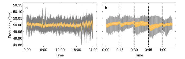
Figure 1: Fluctuations in frequency around the reference frequency of 50Hz a: Box plot of the 2015 data by Réseau de Transport d’Electricité (RTE) RTE-UCTE2016 describing the Continental European power grid. b: Zoom-in on the first 70 minutes of the frequency measurements, exposing substantial changes in average and variance of frequencies at 15 minutes trading intervals (indicated by the dashed lines) . Each box contains data of one year for the same time instance (averaged per minute in a). The yellow bars contain the 25% and 75% quartile, the gray bars are the whiskers giving the maximum and minimum values and the white line is the median value.

In this Article, we analyze the frequency fluctuations observed in several electric power grids from three continents. We determine and characterize the non-Gaussian nature of these fluctuations existing across grids in both the 60Hz and 50Hz operation regimes. Furthermore, we propose an analytically accessible model successfully describing these data in one consistent framework by systematically incorporating the non-Gaussian nature of fluctuations and verify its predictions. The analysis yields trading as a key factor for non-Gaussianity. Extracting the effective damping for different synchronous regions via autocorrelation measures, our work highlights that the effective grid damping as well as the size of the grid itself serve as controlling factors to make grid dynamics more robust. Finally, we demonstrate how superstatistics explains heavy tails and skewness using superimposed Gaussian distributions.

Observing the statistics of Frequency Fluctuations

The bulk frequency of a power grid fluctuates around its nominal frequency of 60 Hz (most parts of America, western Japan, Korea, Philippines) or 50 Hz (eastern Japan and other countries). To understand and quantify these fluctuations, we analyze data sets for the power grid frequency of the European Network of Transmission System Operators for Electricity (ENTSO-E) Continental European (CE) 50Hertz-UCTE2016 ; RTE-UCTE2016 , the Nordic Fingrid2015-2016 , Mallorcan Mallorca2015 and Great Britain (GB) UK-Frequency2016 grids, the 50 Hz and 60 Hz regions of Japan OCCTO-Frequency2016 as well as the Eastern Interconnection (EI) in North America US_Frequency_data , see Supplementary Note 1 for more detailed data breakdown. The data consist of power grid frequency measurements at one location in the given region (two for Continental Europe) at a sampling rate between ten measurements per second and one measurement per five minutes.

At first glance, a typical recording of the grid frequency (Fig. 1) reveals that it coincides extremely well with the nominal grid reference frequency, highlighting the efficiency of today’s frequency control. Only rarely do we observe large deviations from the nominal frequency. These large disturbances often occur when a new power dispatch has been settled on by trading (every 15 minutes), introducing jumps and fluctuations of the frequency. The total variance of the frequency fluctuations in a given region thereby depends on the size of the grid – larger grids are more inertial and thus tend to have a smaller variance.

All distributions deviate from Gaussian distributions, which becomes evident when observing their tails (Fig. 2). For the Continental European, Nordic, Mallorcan and Japanese grids large deviations from the nominal frequency are more frequent than for a Gaussian distribution of given variance, leading to heavy tails, as quantified, for instance, by an excess kurtosis, see Methods. The grids of Great Britain and the Eastern Interconnection however, are substantially skewed, i.e., they are asymmetric around the reference frequency so that deviations towards lower frequencies are more likely than to higher ones.

Lévy-stable Samorodnitsky1994 and q-Gaussian distributions Tsallis2009 are the best fitting distributions among all distributions tested, as identified by a maximum likelihood analysis, see Fig. 2 and Supplementary Note 1. Both distributions generalize a Gaussian distribution to include heavy tails and point to two different microscopic mechanisms underlying the frequency dynamics: q-Gaussians arise when the power fluctuations are Gaussian on short time scales, but with a variance or mean changing on longer time scales. In contrast, Lévy-stable distributions arise when the underlying power fluctuations are heavy-tailed or skewed itself. We investigate both settings in more detail below.

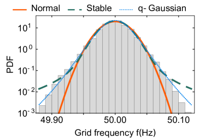
Figure 2: Non-Gaussian nature of the frequency distribution. The 2015 dataset by 50Hertz describing the CE power grid, where fitted normal, stable and q-Gaussian distributions are compared with the histogram data using a log scale for the probability density function (PDF). Deviations from a normal distribution become evident in the tails, which are more pronounced than expected for a normal distribution. The stability parameter of the stable distribution is $\alpha_{S}=1.898\pm 0.002$ and the deformation parameter of the q-Gaussian distribution is $q=1.20\pm 0.01$, whereas ($\alpha_{S}^{\text{Gauss}}$=2 and $q^{\text{Gauss}}$=1 for Gaussian distributions). The Lévy-stable distribution uses four fitting parameters, while the q-Gaussian uses three and the normal distribution uses two parameters.

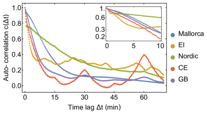
Figure 3: Decay of the autocorrelation of the frequency dynamics. Plotted are autocorrelation measures as a function of time lag $\Delta t$ for the 50Hertz data set for Central Europe (CE) of 2015, the Great Britain grid (GB) of 2015, the Eastern Interconnection (EI) data for 1 day of 2015, the Nordic grid data of 2015 and Mallorcan data of 2015. After an initial decay of the autocorrelation, peaks emerge every 15 minutes due to trading intervals, especially pronounced for the GB and CE grids, consistent with Fig. 1. Using a log-plot in the inset allows to extract the damping of the grid based on the assumption of exponential decay, Equation (1). Note that the CE, GB and EI grids all display similar decay during the initial 5 minutes. In contrast, the Nordic grid displays a fast decay and then a slower one. The plot uses one full year of frequency data with one second resolution for each region to generate the autocorrelation plots. Especially the trading peaks are typically not visible when only 24h of recordings are considered (as for the EI grid).

In addition to the aggregated data, we investigate the autocorrelation of the recorded trajectories, extracting important events and the characteristic time scales during which the system de-correlates. Analyzing the autocorrelation for the Continental European grid reveals pronounced correlation peaks every 15 minutes and especially every 30 and 60 minutes, see Fig. 3. These regular correlation peaks appear in many grids (CE, GB, Nordic) and are explained by the trading intervals in most electricity markets NationalAcademiesofSciences2016 , which are often 30 or 15 minutes. Furthermore, this is also in line with the observation of large deviations in the frequency trajectories, see Fig. 1, so that trading has an important impact on frequency stability. At the beginning of a new trading interval, the production changes nearly instantaneously and the complex dynamical power grid system needs some time to relax to its new operational state.

The decay of the autocorrelation provides further information about the underlying stochastic process. For the first minutes of each trajectory, we observe an exponential decay of the autocorrelation $c$ as a function of the time lag $\Delta t$:

$$c\left(\Delta t\right)\sim\exp\left(-\Delta t/\tau\right),$$ (1)

with a typical correlation time $\tau$, as expected for elementary stochastic processes without memory such as the Ornstein-Uhlenbeck process Gardiner1985 .

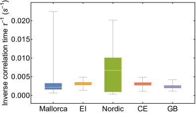
Figure 4: Inverse correlation time of different regions. The box plots display the estimate of the inverse correlation time $\tau^{-1}$ based on the autocorrelation decay fitted by an exponential function, see Equation (1). The data are obtained by evaluating individual days of all years available and splitting the one day of EI into 10 minute trajectories. The box covers the 25% and 75% quartile with the white line being the median while the whiskers give the maximum and minimum values.

We extract the inverse correlation time $\tau^{-1}$ for each available data set and obtain values within the same order of magnitude across all grids, see Fig. 4. The Japanese data set only has measurements every five minutes, hence we refrain from estimating an autocorrelation. The inverse correlation time can be seen as the effective damping $\gamma$ in a synchronous region with $\gamma:=\tau^{-1}$, see below. With this in mind, it is not surprising that all grids return values for $\gamma$ of the same order of magnitude because the synchronous machines in these regions do not differ substantially. This damping consists of mechanical damping, damper windings and primary control.

Stochastic Model of Power Fluctuations

The variations of the grid frequency are driven by fluctuations of power generation and demand. To link the evolution of the grid frequency with the power injections, we make use of the well-established swing equation Filatrella2008 ; Rohden2012 ; Doerfler2013 ; Motter2013 ; Manik2014 ; Kundur1994 ; Machowski2011 ; Dewenter2015 . Aggregating over the grid, we obtain a Fokker-Planck equation that models the observed frequency fluctuations and allows an analytical description of power grid frequency fluctuations.

We analyze frequency dynamics of a power grid on coarse scales. Every node in the grid corresponds to a large generator (power plant) or a coherent subgroup and is characterized by the phase $\theta_{i}$ and the angular velocity $\omega_{i}=2\pi\left(f_{i}-f_{R}\right)$. Here $f_{i}$ denotes the frequency of the nodes $i=1\ldots N$ and $f_{R}=50$Hz or $f_{R}=60$Hz, respectively, is the reference frequency at the grid. The equations of motion of the phase and velocity are then given by

$$\frac{\text{d}}{\text{d}t}\theta_{i} = \omega_{i},$$ (2)

$$M_{i}\frac{\text{d}}{\text{d}t}\omega_{i} = P_{i}+\epsilon_{i}\xi_{i}-D_{i}\omega_{i}+\sum_{j=1}^{N}K_{ij}\sin\left(\theta_{j}-\theta_{i}\right),$$

where we have at each node $i$: inertia $M_{i}$, voltage phase angle $\theta_{i}$, mechanical power $P_{i}$, random noise $\xi_{i}$ with noise amplitude $\epsilon_{i}$, damping $D_{i}$ and the coupling matrix $K_{ij}$ which is determined by the transmission grid topology. The operating state of a power grid is characterized by a stable fixed point of the swing equation (2). The fixed point fulfills $\omega_{i}^{*}=0$ which is equivalent to all machines working at the reference frequency $f_{R}=50$Hz or $f_{R}=60$Hz. At the stable operation point the frequencies at all nodes are equal: $\omega_{i}=\bar{\omega}$. Deviations are only observed during system-wide failures or transiently after serious contingencies or major topology changes Machowski2011 ; Kundur1994 . To obtain the effective equation of motion of the bulk angular velocity $\bar{\omega}$, we assume a homogeneous ratio of damping and inertia throughout the network, $\gamma=D_{i}/M_{i}$ Weixelbraun2009 as well as symmetric coupling $K_{ij}=K_{ji}$ and assume that the power is balanced $\sum_{i=1}^{N}P_{i}=0$ on average Manik2014 . Setting $M:=\sum_{i}M_{i}$, the dynamics of the bulk angular velocity $\bar{\omega}:=\sum_{i=1}^{N}M_{i}\omega_{i}/M$ is governed by the Aggregated Swing Equation (see also Ulbig2014 )

$$\frac{\text{d}}{\text{d}t}\bar{\omega}=-\gamma\bar{\omega}+\bar{\epsilon}\bar{\xi}\left(t\right).$$ (3)

This aggregated swing equation no longer requires precise knowledge of the parameters of a given region but depends on the effective damping $\gamma$, the aggregated noise amplitude $\bar{\epsilon}$ and the statistics of the random noise $\bar{\xi}$, all characterizing the overall frequency dynamics, see Methods and Supplementary Note 2 for details. We note that the damping $\gamma$ integrates contributions from damper windings and primary control actions alike. Finally, both damping $\gamma$ and the noise amplitude $\bar{\epsilon}$ could easily change over time, e.g., due connection of certain grids or day/night differences. We cover this scenario in the section on superstatistics.

The bulk angular velocity $\bar{\omega}$ (and thereby the grid frequency) is not following a deterministic evolution but is influenced by stochastic effects, given by the aggregated power fluctuations $\bar{\xi}$. Hence, we characterize a given grid by the probability distribution function (PDF) of the bulk angular velocity $p\left(\bar{\omega}\right)$, similar to the frequency distribution plotted in Fig. 2. A wide distribution, i.e. one with high standard deviation, or one with heavy tails, i.e., high kurtosis, displays large deviations more often and is thereby less stable than a narrower distribution.

The central decision when modeling stochastic dynamics is how to describe the noise $\xi$ which is generated from some probability distribution. Explicit choices of noise distributions are covered here and in Supplementary Notes 2 and 3 for Gaussian and non-Gaussian noise, respectively and extended to noise drawn from a Gamma distribution Carpaneto2008 ; T.Soubdhan2009 in Supplementary Note 4. Given the distribution of $\xi$, we then formulate and solve a Fokker-Planck equation Gardiner1985 to obtain an analytical description of the distribution of $\bar{\omega}$.

The simplest noise model assumes the noise $\xi_{i}$ as independent Gaussian noise based on the often-used central limit theorem. It states that the sum of independent random numbers drawn from any fixed distribution with finite variance approaches a Gaussian distribution if the sample is sufficiently large Gardiner1985 . In our setting, the sum consists of all contributions to the noise by consumers, renewables, trading etc. The Fokker-Planck equation describing the time-dependent probability density function $p\left(\bar{\omega},t\right)$ follows then as

$$\frac{\partial p}{\partial t}=\gamma\frac{\partial}{\partial\bar{\omega}}\left(\bar{\omega}p\right)+\frac{1}{2}\sum_{i=1}^{N}\frac{\epsilon_{i}^{2}}{M^{2}}\frac{\partial^{2}p}{\partial\bar{\omega}^{2}},$$ (4)

which is the well-known Ornstein-Uhlenbeck process Gardiner1985 . The stationary distribution

$$p\left(\bar{\omega}\right)=\sqrt{\frac{\gamma M^{2}}{\pi\sum_{i=1}^{N}\epsilon_{i}^{2}}}\exp\left[-\bar{\omega}^{2}\frac{\gamma M^{2}}{\sum_{i=1}^{N}\epsilon_{i}^{2}}\right],$$ (5)

of (4) characterizes the steady state of the grid as mathematically defined by $\partial p/\partial t$=0, see Gardiner1985 as well as Methods and Supplementary Notes 2 and 6 for details.

Crucially, Equation (5) is again a Gaussian distribution of $p\left(\bar{\omega}\right)$, i.e., a Gaussian distribution for the power feed-in fluctuations results in a Gaussian frequency distribution. Assuming we know the damping $\gamma$, noise amplitudes $\epsilon_{i}$ and the total inertia $M$, we are able to compute the expected frequency distribution analytically. Furthermore, the Ornstein-Uhlenbeck autocorrelation exactly follows an exponential decay with characteristic time determined by the damping $\tau=1/\gamma$.

Under which conditions do we need to include non-Gaussian effects in the stochastic modeling? When applying the central limit theorem, one explicitly assumes finite variance. However, solar and wind fluctuations are known to display heavy tails Anvari2016 ; Milan2013 and contribute to the fluctuations in the power grid. Hence, to describe deviations from normal distributions, including heavy tails and skewed distributions, we need to base the input noise $\xi$ on a non-Gaussian noise generating process Denisov2009 . This requires generalized Fokker-Planck equations, see Supplementary Note 3. These generalized equations characterize fluctuations based on noise input distributed according to, e.g., a Lévy-stable law. These Lévy-stable distributions include heavy tails and skewed distributions, as often observed in nature Peinke2004 and are a reasonable fit for the frequency data, see Fig. 2. Stable distributions are characterized by a stability parameter $\alpha_{S}\in(0,2]$, which determines the heavy tails, a skewness parameter $\beta_{S}$ and a scale parameter $\sigma_{S}$, which is similar to the standard deviation for Gaussian distributions Samorodnitsky1994 .

Inputting power fluctuations $\xi$ drawn from a stable distribution into the stochastic Equation (3) also results in grid frequency fluctuations characterized by a stable distribution, considered as the ’output’ of Equation (3). Between input and output distributions, only the scale parameter is modified whereas the skewness $\beta_{S}$ (asymmetry) and the stability parameter $\alpha_{S}$ (heavy-tail-ness) are preserved. In particular, the scale parameter $\sigma_{S}^{\text{in}}$ of the input distribution changes to that of the output distribution $\sigma_{S}^{\text{out}}$ following the map (Supplementary Notes 3 and 6)

$$\sigma_{S}^{\text{in}}=\frac{1}{\sqrt{2}M}\left[\sum_{i=1}^{N}\epsilon_{i}^{\alpha_{S}}\right]^{1/\alpha_{S}}\mapsto\,\sigma_{S}^{\text{out}}=\frac{\sigma_{S}^{\text{in}}}{\left(\gamma\alpha_{S}\right)^{1/\alpha_{S}}}.$$ (6)

We emphasize this remarkable and unique property of stable distributions Samorodnitsky1994 for linear models: If the input power fluctuations are distributed according to a stable distribution, the output frequency fluctuations are distributed according to the same family of distributions, with only one parameter transformed. This property holds for any linear stochastic process, including the aggregated swing equation (3). The same happens for Gaussian distributions since they constitute a subclass of stable distributions in the limit $\alpha_{S}\rightarrow 2$. These properties are in stark contrast to those of non-stable distributions, see Supplementary Notes 3 and 4.

What are the consequences of relation (6)? Making the output frequency distribution narrower, i.e., reducing risks of extreme events, requires $\sigma_{S}^{\text{out}}$ to be as small as possible. However, increasing the share of renewables by rebuilding the energy system is expected to increase the noise amplitudes $\epsilon_{i}$. In addition, trading impacts the frequency fluctuations and thereby also contributes to the noise amplitudes (Fig. 1). However, fluctuations are efficiently reduced by increasing the effective damping $\gamma$ or the inertia $M$, see Eq. (6).

With the previous results, we are able to quantify the intuitive statement that larger regions have more inertia and hence narrower distributions by explicitly comparing the scale parameters (proportional to standard deviations in the case of $\alpha_{S}=2$) of two different regions as follows:

$$\sigma_{S\,2}^{\text{out}}=\sigma_{S\,1}^{\text{out}}\frac{m_{1}}{m_{2}}\left(\frac{\gamma_{1}N_{1}^{\alpha_{S}-1}}{\gamma_{2}N_{2}^{\alpha_{S}-1}}\right)^{1/\alpha_{S}},$$ (7)

assuming identical stability parameters $\alpha_{S}$ and average inertia $m_{\mu}=M_{\mu}/N_{\mu},\,\mu\in\left\{1,2\right\}$. Equation (7) shows that a smaller region ($N_{2}<N_{1}$) needs larger damping than a larger region ($\gamma_{2}\overset{!}{>}\gamma_{1}$) or has a broader distribution with $\sigma_{S\,2}^{\text{out}}>\sigma_{S\,1}^{\text{out}}$, i.e., a higher risk of large deviations from the stable operational range. The scaling is given by the scale parameter $\sigma_{S}\sim N^{\left(\alpha_{S}-1\right)/\alpha_{S}}$, where the simple square root law is recovered only in the case of Gaussian distributions $\left(\alpha_{s}=2\right)$. Also, it reveals that decreasing inertia proportionally increases the scale parameter.

Furthermore, we estimate the order of magnitude of the expected noise amplitude

$$\epsilon=\sigma_{S}^{\text{out}}m\left(\alpha_{S}\gamma N^{\alpha_{S}-1}\right)^{1/\alpha_{S}}.$$ (8)

by computing the scaling from (6) for typical noise contributions of the order of $\epsilon_{i}=\epsilon$. Based on pure frequency measurements, every quantity is available for each synchronous region: We estimate the output scale parameter $\sigma_{S}^{\text{out}}$ and stability parameter $\alpha_{S}$ from the histogram data. We assume that the number of nodes $N$ is directly proportional to the total electricity production of a region per year ENTSO-EProductionData2016 ; EIA-411EnergyReport2016 . Since a process driven by stable noise has no defined autocorrelation function Samorodnitsky1994 , we approximate its autocorrelation with the Ornstein-Uhlenbeck process and thereby derive an estimate for the damping $\gamma$. With these estimates and Equation (8) we plot the noise amplitudes for different regions in Fig. 5. The estimated noise amplitude tends to increase with increasing share of intermittent renewable generation (wind and solar) in a given region. Nevertheless, this relationship is not very strict and frequency disturbances at trading intervals, see Fig. 1 demonstrate, that at least today trading and demand fluctuations are contributing substantially to frequency fluctuations.

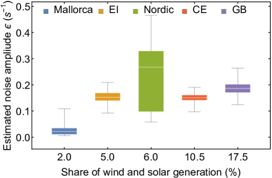
Figure 5: Noise amplitudes for European and American grids. The noise amplitude tends to increase with the shares of intermittent renewables. The noise amplitude $\epsilon$ for each grid is calculated assuming that it is identical at each node $\epsilon_{i}=\epsilon$ and assuming homogeneous inertia. The power production is normalized with respect to the Eastern Interconnection (EI) generation for the ENTSO-E grids of Continental Europe (CE), Mallorca, Nordic and Great Britain (GB). Frequency data of all regions and Equation (8) is used to compute the noise amplitude $\epsilon$ which we expect to be similar in all regions, providing a self-consistency check of our theory. The box plot is obtained by using different damping, standard deviation estimates, etc. for each day of multiple years. The data for the Nordic grid has large uncertainty due to the two different correlation time scales. See Supplementary Note 1 for details on the data.

Superstatistics

Instead of modeling the underlying stochastic process as non-Gaussian, we may interpret the observed statistic as a superposition of multiple Gaussians, leading to superstatistics, explaining heavy tails and skewness Beck2003 ; Chechkin2017 .

For our superstatistical approach we use Equation (3) with Gaussian noise $\bar{\xi}$

$$\frac{\text{d}}{\text{d}t}\bar{\omega}=-\gamma\bar{\omega}+\bar{\epsilon}\bar{\xi}\left(t\right),$$ (9)

which yields a Gaussian distribution, see Eq. (5).

What changes when the damping $\gamma$ is no longer constant over time? Both control actions and physical damping contribute to $\gamma$ and change over time when certain power plants are connected and others are shut down. Similarly, the noise amplitude $\bar{\epsilon}$ of the system depends on which consumers are currently active, whether it is day or night, which renewables are connected and more. Hence, it is appropriate to replace our static parameters $\gamma$ and $\bar{\epsilon}$ by dynamical parameters that change over time with a typical time scale $T$. When applying superstatistics, we assume that the time scale $T$ is large compared to the intrinsic time scale of the system, which is given by the autocorrelation time scale, namely $T\gg\tau=1/\gamma$. Then, the stochastic process finds an equilibrium with an approximately Gaussian distribution determined by the current noise and damping. When these parameters change, the frequency distribution becomes a Gaussian distribution with different standard deviation. In Fig. 6a we demonstrate how just a few Gaussian distributions with different standard deviations give rise to an excess kurtosis and in Supplementary Note 5 we show how two Gaussian distributions with shifted means result in a skewed distribution.

We extract the long time scale $T$ from the data and compare it to the intrinsic short time scale of the system. The short time scale $\tau=1/\gamma$ is based on the exponential decay of the autocorrelation of the time series of $\bar{\omega}$ yielding a range of $\tau\approx 200...550\,s$ for all grids. The long time scale $T$ is governed by the idea that the superstatistical ensemble has heavier tails than a normal distribution but that for a given typical time scale $T$ an equilibrium distribution emerges that is approximately Gaussian. Given a time series $x\left(t\right)$ with mean $\bar{x}$, we compute the local kurtosis $\kappa\left(\Delta t\right)$ for different time intervals $\Delta t$ and choose the large time scale $T$ by $\kappa\left(\Delta t=T\right)=3$ Beck2003 . Similarly, we compute the time for which the average skewness is zero to extract the long time scale for the Great Britain or Eastern Interconnection grids, see Methods and Supplementary Note 5 for details and Fig. 6 for an example for Japan.

Figure 6: Superimposed Gaussian distributions leading to heavy tails. a: When the stochastic process follows two different Gaussian distributions (orange and green) and the data is aggregated (gray histogram), the result is a heavy-tailed distribution which is not Gaussian. Consequently, Gaussian fits (blue curve) tend to underestimate its tails. Assuming such a structure for the real frequency measurements, the frequency recordings are split into trajectories of length $\Delta t$ each and the kurtosis is computed. b: The average kurtosis of the Japanese 60Hz data set in dependence of the length of $\Delta t$. For very small $\Delta t$ the distribution has lighter tails than a Gaussian while using the full data set or large $\Delta t$ leads to the earlier observed heavy tails. The long time scale $T$, during which the distribution changes, is determined as $\kappa\left(\Delta t=T\right)=3$.

All synchronous regions return large but different long time scales $T$. We determine the long time scales to be of the order of $T\approx 1\ldots 5\,h$ with small values in Mallorca and the Eastern Interconnections and large values in Continental Europe and Japan, hinting to distinct underlying mechanisms how damping and noise change in each region. Compared to the intrinsic short time scale $\tau\sim 200...550\,s$, the long time scale $T$ is larger by at least one order of magnitude. Hence, the superstatistical approach is justified, i.e., it is valid to interpret the heavy tails as a result of superimposing Gaussians.

Finally, we perform another consistency check of the superstatistical approach and extract the distribution of the effective friction $\gamma_{\text{eff}}$ Beck2003 , see Methods. Based on general results on superstatistics, we expect the effective friction to follow a $\chi^{2}$, inverse $\chi^{2}$ or log-normal distribution Clark1973 ; B.Castaing1990 , which then leads to an approximate q-Gaussian distribution of the frequency, see Supplementary Note 5 for a derivation. In the case of the Japanese 60Hz region the distribution of $\gamma_{\text{eff}}$ is well-described by a log-normal distribution again supporting the superstatistical approach, see Fig. 7.

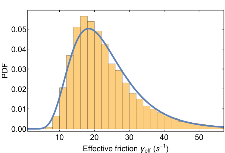
Figure 7: Self-consistency test of superstatistics. Plotted is the histogram of the effective friction $\gamma_{\text{eff}}$ based on the Japanese 60Hz frequency measurements which is well-described by a log-normal distribution. Such a distribution of the effective friction $\gamma_{\text{eff}}$, directly leads to q-Gaussian distributions of the aggregated data, see Supplementary Note 5. Other data sets are also approximated by log-normal distributions, see Supplementary Note 5.

Discussion

In summary, we have analyzed power grid frequency fluctuations by applying analytical stochastic methods to time series of different synchronous regions across continents including North America, Japan and different European regions. Based on bulk frequency measurements, we have identified trading as a substantial source of fluctuations (Figs. 1 and 3). Although frequency fluctuations and power uncertainty are often modeled as Gaussian distributions Wood2012 ; Jin2005 ; Zhang2010 ; Schaefer2017 ; Fang2012 , we pinned down and quantified substantial deviations from a Gaussian form, including heavy tails and skewed distributions (Fig. 2).

Obtaining an analytical description of a complex system allows deeper insight into it. Hence, condensing the analysis of frequency fluctuations in power grids via a second order nonlinear dynamics, the swing equation, and neglecting spatial correlations, we derived (generalized) Fokker-Planck equations for the bulk angular velocity $\bar{\omega}$. We obtained precise predictions on how power fluctuations impact the distribution of fluctuations of the grid frequency. Furthermore, our approach identifies, besides grid size, an increasing effective damping and inertia as a controlling factor for reducing fluctuation-induced risks. By incorporating smart grid control mechanisms Schaefer2015 or increasing generator droop control Machowski2011 , modifying effective damping may therefore reliably reduce the likelihood of large fluctuations in power grids Schoell2008 . Finally, our analytical theory is able to compare differently sized grids, predict fluctuations based on the size and inertia of the grid (Equation (7)). Crucially, our mathematical framework goes beyond the simple $N^{-1/2}$ scaling of Gaussian noise.

The results offer two approaches to model power grids under uncertainty: First, an optimization could include the non-Gaussian nature of the distribution by incorporating non-Gaussian noise, e.g. in the form of Lévy-stable noise. Alternatively, we demonstrated that the distributions are also well explained by a superstatistics approach where the non-Gaussian nature of the distributions arises by superimposing different Gaussian distributions. Especially when modeling shorter time scales of one hour or below, a Gaussian approach is supported by our results. Studies aiming to cover time scales of full months or years, however, have to account for changing mean and variance of the assumed Gaussian distribution or explicitly model non-Gaussian distributions, going beyond current Gaussian approaches Wood2012 ; Jin2005 ; Zhang2010 ; Schaefer2017 ; Fang2012 .

The findings reported above have a number of implications for the operation and design of current and future energy systems. First, as trading induces large frequency fluctuations, designing new electricity markets and limiting frequency fluctuations are highly interlinked, especially when considering the implementation of smart grid concepts Fang2012 ; Schaefer2015 . Second, knowing the temporal correlation structure of fluctuations helps predicting increasing and decreasing likelihoods of large amplitude events, thereby enabling mitigation strategies to be applied on time scales that make them most efficient. Finally, deriving the scaling of fluctuations as a function of grid parameters, especially the grid size, should be very useful when setting up isolated grids, e.g. microgrids with a specified frequency quality as damping and control needs can easily be estimated by the approach introduced above. This may also be of use for larger synchronous regions when facing a decreasing inertia $M$.

Moreover, applying similar stochastic methods to power grids also raises a range of additional questions: How does correlated noise impact the frequency statistics? Does the predicted scaling of fluctuations with the grid size hold for a larger collection of independent power grids and in particular very small islands or microgrids? Can we disentangle damping and primary control to explain the differences of long time scales among different regions? These questions require further careful data analysis in future work, involving substantially more data of microgrids, work that could inspire further collaboration including a range of academic fields as well as public institutions and industry.

Methods

Moments of the frequency distributions

Deviations from Gaussian distributions as observed in Fig. 2 are quantified in a model independent way using moments of the frequency distribution: Given $M$ measurements of a discrete stochastic variable $f$, e.g. the grid frequency, as $f_{1}$, $f_{2}$,…,$f_{M}$, its $n$-th moment is defined as

$$\mu_{n}:=\frac{1}{M}\sum_{i=1}^{M}f_{i}^{n}.$$ (10)

The first moment of a distribution is the mean $\mu_{1}\equiv\mu$. Instead of the second moment, the centralized second moment, i.e., the variance is more commonly used. It is defined as

$$\sigma^{2}:=\frac{1}{M}\sum_{i=1}^{M}\left(f_{i}-\mu\right)^{2}.$$ (11)

Finally, we use the normalized third and fourth moments, the skewness $\beta$ and kurtosis $\kappa$, respectively, which are defined as

$$\beta := \frac{1}{M}\sum_{i=1}^{M}\left(\frac{f_{i}-\mu}{\sigma}\right)^{3},$$ (12)

$$\kappa := \frac{1}{M}\sum_{i=1}^{M}\left(\frac{f_{i}-\mu}{\sigma}\right)^{4}.$$ (13)

A Gaussian distribution is symmetric and hence the skewness $\beta$ equals zero. A non-zero skewness implies a distribution that is not symmetric around the mean but is more pronounced in one direction. The kurtosis meanwhile quantifies the extremity of the tails. A Gaussian distribution has $\kappa^{\text{Gauss}}=3$ while a higher value indicates an increased likelihood of large deviations. For instance, the continental European grid displays a kurtosis of $\kappa^{\text{CE}}=4.0\pm 0.1$.

Normally distributed noise

For Eq. (4) we took the sum over multiple noise realizations that follow a normal distribution: Let $\xi_{i}$ be random variables following a normal distribution, i.e.,

$$\xi_{i}\sim N\left(0,1\right),$$ (14)

where $N\left(0,1\right)$ denotes a normal distribution with mean $0$ and standard deviation $1$. Then, the sum of identically and independently distributed random variables $\xi_{i}$ given as

$$\bar{\epsilon}\bar{\xi}:=\sum_{i=1}^{N}\epsilon_{i}\xi_{i}$$ (15)

is distributed like a single normal distribution Samorodnitsky1994

$$\bar{\epsilon}\bar{\xi}\sim N\left(0,\sqrt{\sum_{i=1}^{N}\epsilon_{i}^{2}}\right).$$ (16)

Superstatistics

In Figs. 6 and 7 we extract the local kurtosis and effective damping from the time series as follows. Let $x\left(t\right)$ be a time series of random measurements with a mean $\bar{x}$. To test whether $x\left(t\right)$ is aggregated by drawing from multiple distributions, we compute the local kurtosis as:

$$\kappa\left(\Delta t\right)=\frac{1}{t_{\text{max}}-\Delta t}\int_{0}^{t_{\text{max}}-\Delta t}\frac{\left\langle\left(x-\bar{x}\right)^{4}\right\rangle_{t_{0},\Delta t}}{\left\langle\left(x-\bar{x}\right)^{2}\right\rangle_{t_{0},\Delta t}^{2}}\text{d}t_{0},$$ (17)

where $\left\langle...\right\rangle_{t_{0},\Delta t}=\int_{t_{0}}^{t_{0}+\Delta t}...\text{d}t$. We do so for several values of $\Delta t$ and choose $T$ so that $\kappa\left(\Delta t=T\right)=3$, i.e., averaging over a time scale $T$ , there is no excess kurtosis and locally the variable $x$ is subject to Gaussian noise.

The effective friction $\gamma_{\text{eff}}$, which is changing over time, is then computed as

$$\gamma_{\text{eff}}\left(t_{0}\right)=\frac{1}{\left\langle x^{2}\right\rangle_{t_{0},T}-\left\langle x\right\rangle_{t_{0},T}^{2}}.$$ (18)

Following Beck2003 we expect $\gamma_{\text{eff}}$ to follow a log-normal or alternatively a $\chi^{2}$ or inverse $\chi^{2}$ distribution as those lead to q-Gaussian distributions of $x$, see Supplementary Note 5.

Data availability

Frequency recordings are publicly available at the respective references for the CE, GB, Nordic and Japanese regions 50Hertz-UCTE2016 ; RTE-UCTE2016 ; Fingrid2015-2016 ; UK-Frequency2016 ; OCCTO-Frequency2016 . Frequency data for Mallorca Mallorca2015 were provided by Eder Batista Tchawou Tchuisseu. Data for the Eastern Interconnection US_Frequency_data were provided by Micah Till. All data that support the results presented in the figures of this study are available from the authors upon reasonable request.

Author contributions

B.S., D.W. and M.T. conceived and designed the research. B.S. acquired the data, performed the data analysis and formulated stochastic predictions. All authors contributed to discussing the results and writing the manuscript.

Competing interests

The authors declare no competing interests.

References

- (1) The 21st Conference of the Parties to the United Nations Framework, Convention on Climate Change (UNFCCC). The Paris Agreement (2015). URL http://unfccc.int/paris_agreement/items/9485.php.
- (2) Intergovernmental Panel on Climate Change. Climate Change 2014–Impacts, Adaptation and Vulnerability: Regional Aspects (Cambridge University Press, 2014).
- (3) Jacobson, M. Z. & Delucchi, M. A. Providing all global energy with wind, water, and solar power, Part I: Technologies, energy resources, quantities and areas of infrastructure, and materials. Energy Policy 39, 1154–1169 (2011).
- (4) Schäfer, B., Matthiae, M., Timme, M. & Witthaut, D. Decentral Smart Grid Control. New Journal of Physics 17, 015002 (2015).
- (5) Turner, J. A. A Realizable Renewable Energy Future. Science 285, 687–689 (1999).
- (6) Boyle, G. Renewable Energy (Oxford University Press, Oxford, 2004).
- (7) Ueckerdt, F., Brecha, R. & Luderer, G. Analyzing major challenges of wind and solar variability in power systems. Renewable Energy 81, 1–10 (2015).
- (8) Heide, D. et al. Seasonal Optimal Mix of Wind and Solar Power in a Future, Highly Renewable Europe. Renewable Energy 35, 2483–2489 (2010).
- (9) Milan, P., Wächter, M. & Peinke, J. Turbulent Character of Wind Energy. Physical Review Letters 110, 138701 (2013).
- (10) Peinke, J. et al. Fat tail statistics and beyond. In Advances in Solid State Physics, 363–373 (Springer, 2004).
- (11) Machowski, J., Bialek, J. & Bumby, J. Power System Dynamics: Stability and Control (John Wiley & Sons, 2011).
- (12) Kundur, P., Balu, N. J. & Lauby, M. G. Power system stability and control, vol. 7 (McGraw-hill New York, 1994).
- (13) Ulbig, A., Borsche, T. S. & Andersson, G. Impact of low rotational inertia on power system stability and operation. IFAC Proceedings Volumes 47, 7290–7297 (2014).
- (14) Delille, G., Francois, B. & Malarange, G. Dynamic frequency control support by energy storage to reduce the impact of wind and solar generation on isolated power system’s inertia. IEEE Transactions on Sustainable Energy 3, 931–939 (2012).
- (15) Doherty, R. et al. An assessment of the impact of wind generation on system frequency control. IEEE Transactions on Power Systems 25, 452–460 (2010).
- (16) Wood, A. J. & Wollenberg, B. F. Power generation, operation, and control (John Wiley & Sons, 2012).
- (17) National Academies of Sciences Engineering and Medicine. The Power of Change: Innovation for Development and Deployment of Increasingly Clean Electric Power Technologies (The National Academies Press, 2016).
- (18) Jin, Y. & Branke, J. Evolutionary optimization in uncertain environments - a survey. IEEE Transactions on Evolutionary Computation 9, 303–317 (2005).
- (19) Zhang, H. & Li, P. Probabilistic analysis for optimal power flow under uncertainty. IET Generation, Transmission & Distribution 4, 553–561 (2010).
- (20) Schäfer, B. et al. Escape routes, weak links, and desynchronization in fluctuation-driven networks. Physical Review E 95, 060203 (2017).
- (21) Fang, X., Misra, S., Xue, G. & Yang, D. Smart Grids - The new and improved Power Grid: A Survey. Communications Surveys & Tutorials, IEEE 14, 944–980 (2012).
- (22) Kashima, K., Aoyama, H. & Ohta, Y. Modeling and linearization of systems under heavy-tailed stochastic noise with application to renewable energy assessment. In 2015 54th IEEE Conference on Decision and Control (CDC), 1852–1857 (IEEE, 2015).
- (23) Mühlpfordt, T., Faulwasser, T. & Hagenmeyer, V. Solving stochastic AC power flow via polynomial chaos expansion. In 2016 IEEE Conference on Control Applications (CCA), 70–76 (IEEE, 2016).
- (24) Anvari, M. et al. Short term fluctuations of wind and solar power systems. New Journal of Physics 18, 063027 (2016).
- (25) Schmietendorf, K., Peinke, J. & Kamps, O. On the stability and quality of power grids subjected to intermittent feed-in. Preprint at https://arxiv.org/abs/1307.2748 (2016).
- (26) Li, X., Hui, D. & Lai, X. Battery energy storage station (BESS)-based smoothing control of photovoltaic (PV) and wind power generation fluctuations. IEEE Transactions on Sustainable Energy 4, 464–473 (2013).
- (27) Lauby, M. G., Bian, J. J., Ekisheva, S. & Varghese, M. Frequency response assessment of ERCOT and Québec interconnections. In 2014 North American Power Symposium (NAPS), 1–5 (IEEE, 2014).
- (28) Lasseter, R. H. & Paigi, P. Microgrid: A conceptual solution. In 2004 IEEE 35th Annual Power Electronics Specialists Conference (PESC), vol. 6, 4285–4290 (IEEE, 2004).
- (29) Réseau de Transport d’Electricité (RTE). Network frequency (2014-2016). URL https://clients.rte-france.com/lang/an/visiteurs/vie/vie_frequence.jsp.
- (30) 50Hertz Transmission GmbH. ENTSO-E Netzfrequenz. http://www.50hertz.com/de/Maerkte/Regelenergie/Regelenergie-Downloadbereich (2010-2016).
- (31) Fingrid. Nordic power system frequency measurement data (2015-2016). URL http://www.fingrid.fi/en/powersystem/Power%20system%20management/Maintaining%20of%20balance%20between%20electricity%20consumption%20and%20production/Frequency%20measurement%20data/Pages/default.aspx.
- (32) Tchuisseu, E. B., Gomila, D., Brunner, D. & Colet, P. Effects of dynamic-demand-control appliances on the power grid frequency. Preprint at https://arxiv.org/abs/1704.01638 (2017).
- (33) National Grid. Frequency data. http://www2.nationalgrid.com/Enhanced-Frequency-Response.aspx (2014-2016).
- (34) Organization for Cross-regional Coordination of Transmission Operators, Japan (OCCTO). Japanese grid frequency (2016). URL http://occtonet.occto.or.jp/public/dfw/RP11/OCCTO/SD/LOGIN_login#.
- (35) Power Information Technology Lab, University of Tennessee, Knoxville and Oak Ridge National Laboratory. FNET/GridEye (2014). URL http://powerit.utk.edu/fnet.html. 1 day data set "20140905".
- (36) Samorodnitsky, G. & Taqqu, M. S. Stable Non-Gaussian Random Processes. Stochastic Models with Infinite Variance (Chapman and Hall, 1994).
- (37) Tsallis, C. Nonadditive entropy and nonextensive statistical mechanics - an overview after 20 years. Brazilian Journal of Physics 39, 337–356 (2009).
- (38) Gardiner, C. W. Handbook of stochastic methods (Springer Berlin, 1985), 3 edn.
- (39) Filatrella, G., Nielsen, A. H. & Pedersen, N. F. Analysis of a Power Grid using a Kuramoto-like Model. The European Physical Journal B 61, 485–491 (2008).
- (40) Rohden, M., Sorge, A., Timme, M. & Witthaut, D. Self-organized Synchronization in Decentralized Power Grids. Physical Review Letters 109, 064101 (2012).
- (41) Dörfler, F., Chertkov, M. & Bullo, F. Synchronization in Complex Oscillator Networks and Smart Grids. Proceedings of the National Academy of Sciences 110, 2005–2010 (2013).
- (42) Motter, A. E., Myers, S. A., Anghel, M. & Nishikawa, T. Spontaneous Synchrony in Power-grid Networks. Nature Physics 9, 191–197 (2013).
- (43) Manik, D. et al. Supply Networks: Instabilities without Overload. The European Physical Journal Special Topics 223, 2527–2547 (2014).
- (44) Dewenter, T. & Hartmann, A. K. Large-deviation properties of resilience of power grids. New Journal of Physics 17, 015005 (2015).
- (45) Weixelbraun, M., Renner, H., Schmaranz, R. & Marketz, M. Dynamic simulation of a 110-kV-network during grid restoration and in islanded operation. In 20th International Conference and Exhibition on Electricity Distribution-Part 1, 2009, 1–4 (IET, 2009).
- (46) Carpaneto, E. & Chicco, G. Probabilistic characterisation of the aggregated residential load patterns. IET Generation, Transmission & Distribution 2, 373–382 (2008).
- (47) Soubdhan, T., Emilion, R. & Calif, R. Classification of daily solar radiation distributions using a mixture of dirichlet distributions. Solar Energy 83, 1056–1063 (2009).
- (48) Denisov, S., Horsthemke, W. & Hänggi, P. Generalized Fokker-Planck equation: Derivation and exact solutions. The European Physical Journal B 68, 567–575 (2009).
- (49) ENTSO-E. Monthly production for a specific year for 2015. https://www.entsoe.eu/db-query/production/monthly-production-for-a-specific-year (2016).
- (50) U.S. Department of Energy. Eia-411: Coordinated bulk power supply and demand program report (2016). URL https://www.eia.gov/electricity/data/eia411/.
- (51) Beck, C. & Cohen, E. G. D. Superstatistics. Physica A 322, 267–275 (2003).
- (52) Chechkin, A. V., Seno, F., Metzler, R. & Sokolov, I. M. Brownian yet non-gaussian diffusion: from superstatistics to subordination of diffusing diffusivities. Physical Review X 7, 021002 (2017).
- (53) Clark, P. K. A subordinated stochastic process model with finite variance for speculative prices. Econometrica: Journal of the Econometric Society 135–155 (1973).
- (54) Castaing, B., Gagne, Y. & Hopfinger, E. Velocity probability density functions of high reynolds number turbulence. Physica D 46, 177–200 (1990).
- (55) Schöll, E. & Schuster, H. G. Handbook of chaos control (2008).
Acknowledgements.
We gratefully acknowledge support from the Federal Ministry of Education and Research (BMBF grant no. 03SF0472A-F to M.T. and D.W.), the Helmholtz Association (via the joint initiative “Energy System 2050 - A Contribution of the Research Field Energy” and the grant no.VH-NG-1025 to D.W.), the Göttingen Graduate School for Neurosciences and Molecular Biosciences (DFG Grant GSC 226/2) to B.S., the EPSRC via the grant EP/N013492/1 to C.B., the JST CREST, Grant Numbers JPMJCR14D2, JPMJCR15K1 to K.A. and the Max Planck Society to M.T.Author contributions