Aligning Points to Lines:
Provable Approximations
Abstract
We suggest a new optimization technique for minimizing the sum of non-convex real functions that satisfy a property that we call piecewise log-Lipschitz. This is by forging links between techniques in computational geometry, combinatorics and convex optimization. As an example application, we provide the first constant-factor approximation algorithms whose running-time is polynomial in for the fundamental problem of Points-to-Lines alignment: Given points and lines on the plane and , compute the matching and alignment (rotation matrix and a translation vector ) that minimize the sum of Euclidean distances between each point to its corresponding line.
This problem is non-trivial even if and the matching is given. If is given, the running time of our algorithms is , and even near-linear in using core-sets that support: streaming, dynamic, and distributed parallel computations in poly-logarithmic update time. Generalizations for handling e.g. outliers or pseudo-distances such as -estimators for the problem are also provided.
Experimental results and open source code show that our provable algorithms improve existing heuristics also in practice. A companion demonstration video in the context of Augmented Reality shows how such algorithms may be used in real-time systems.
Index Terms:
Approximation Algorithms, Non-Convex Optimization, Visual Tracking, Points-to-Lines Alignment, Coresets1 Introduction
We define below the general problem of minimizing sum of piecewise log-Lipschitz functions, and then suggest an example application.
Minimizing sum of piecewise log-Lipschitz functions.
We consider the problem of minimizing the sum over of a set of real non-negative functions that may not be convex but satisfy a property called the piecewise log-Lipschitz property as in Definition 2.
More generally, we wish to minimize the cost function where is a log-Lipschitz function as in Definition 1, and is the set of piecewise log-Lipschitz functions in .
As an application, we reduce the following problem to minimizing such a set of functions.
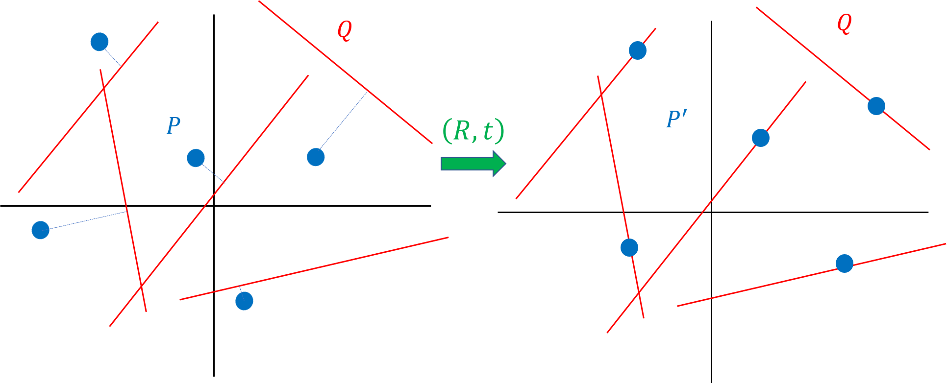
Points-to-Lines alignment
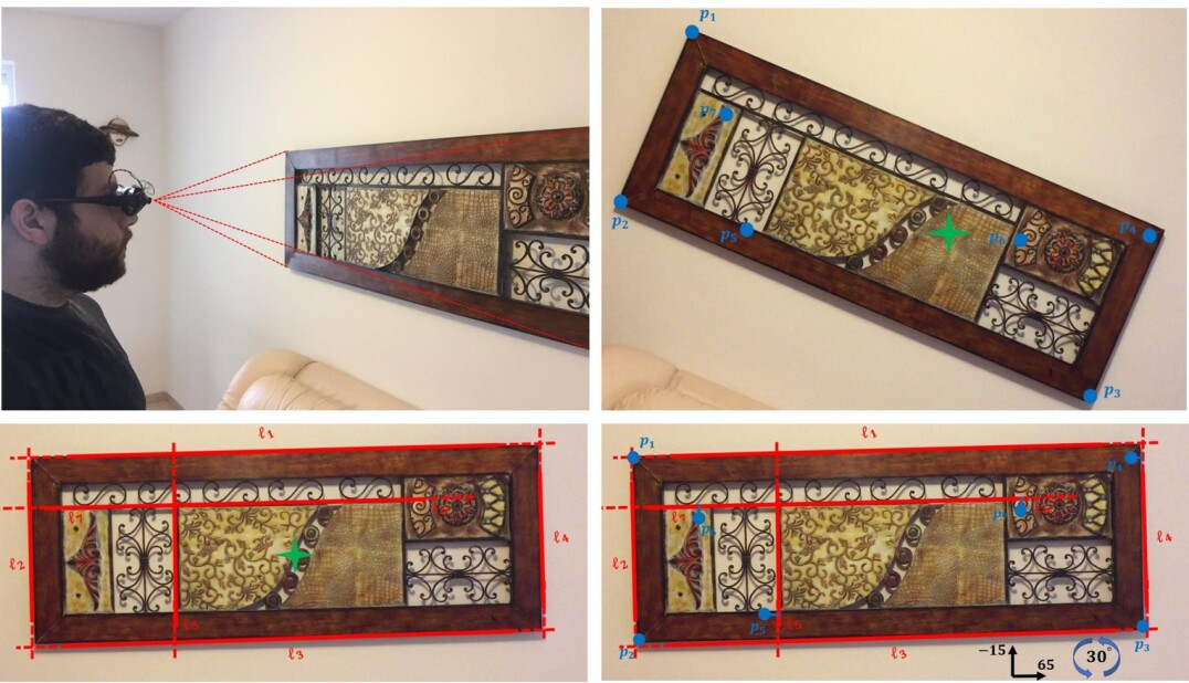
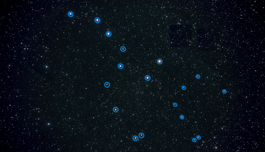
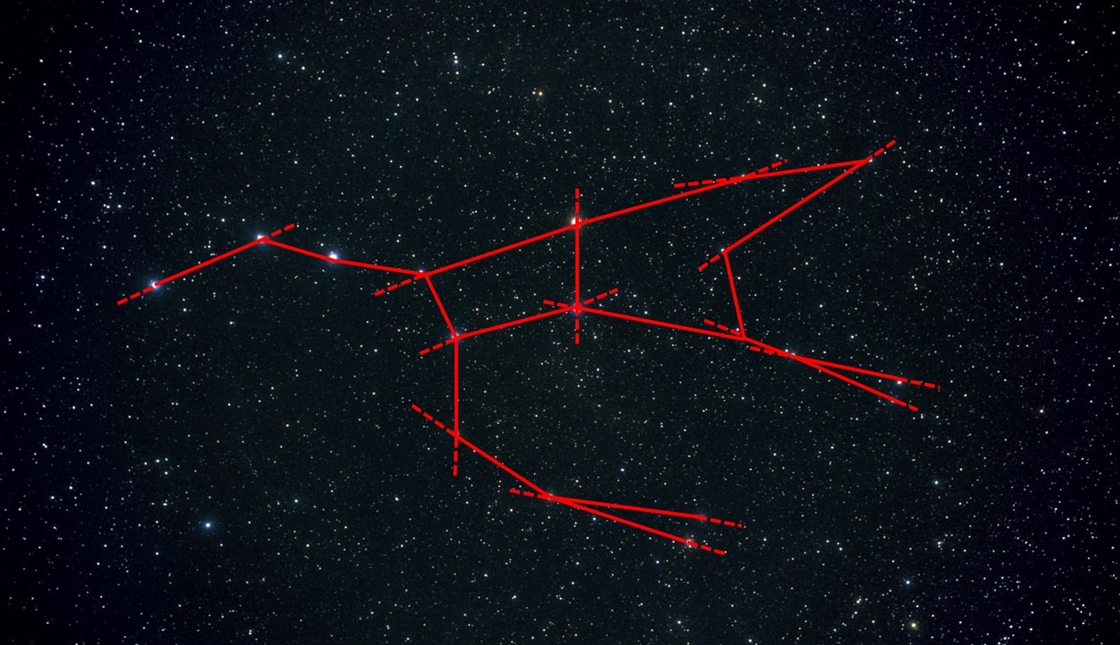
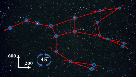
is a fundamental problem in computational geometry, and is a direct generalization of the widely known problem of point set registration, where one is required to align to sets of points; see [1] and references therein. The alignment of points to lines is also known as the Perspective-n-Point (PnP) problem from computer vision, which was first introduced in [2], which aims to compute the position of an object (formally, a rigid body) based on its position as detected in a 2D-camera. Here, we assume that the structure of the object (its 3D model) is known. This problem is equivalent to the problem of estimating the position of a moving camera, based on a captured 2D image of a known object, which is strongly related to the very common procedure of “camera calibration” that is used to estimate the external parameters of a camera using a chessboard. More example applications include object tracking and localization, localization using sky patterns and many more; see Fig. 1, 2 and 3
Formally, the input to these problems is an ordered set of lines that intersect at the origin and an ordered set of points, both in . Each line represents a point in the 2D image. The output is a pair of rotation matrix and translation vector that minimizes the sum of Euclidean distances over each point (column vector) and its corresponding line, i.e.,
| (1) |
where the minimum is over every rotation matrix and translation vector . Here, is the Euclidean distance but in practice we may wish to use non-Euclidean distances, such as distances from a point to the intersection of its corresponding line with the camera’s image plane.
While dozens of heuristics were suggested over the recent decades, to our knowledge, this problem is open even when the points and lines are on the plane, e.g. when we wish to align a set of GPS points to a map of lines (say, highways).
We tackle a variant of this problem, when both the points and lines are in , and the lines do not necessarily intersect at the origin.
1.1 Generalizations
We consider more generalizations of the above problem as follows.
Unknown matching
is the case where the matching between the th point to its line in the PnP problem (1) is not given for every . E.g., in the PnP problem there are usually no labels in the observed images. Instead, the minimization is over every pair of rotation and translation and matching (bijective function) ,
| (2) |
where is the index of the line corresponding to the th point .
Non-distance functions
where for an error vector that corresponds to the input point-line pairs given some candidate solution, the cost that we wish to minimize over all these solutions is where is a log-Lipschitz function as in Definition 1. Special cases include for “worst case” error, which is more robust to noisy data, or of squared distances for maximizing likelihood in the case of Gaussian noise. As in the latter two cases, the function may not be a distance function.
Robustness to outliers
may be obtained by defining to be a function that ignores or at least puts less weight on very large distances, maybe based on some given threshold. Such a function is called an M-estimator and is usually a non-convex function. M-estimators are in general robust statistics functions, such as the well known Huber loss function; see [4].
Coreset
in this paper refers to a small representation of the paired input point-line sets and by a weighted (scaled) subset. The approximation is multiplicative factor, with respect to the cost of any item (query). E.g. in (1) the item (query) is a pair of rotation matrix and translation vector . Composable coresets for this problem have the property that they can be merged and re-reduced; see e.g. [5, 6].
Our main motivation for using existings coresets is (i) to reduce the running time of our algorithms from polynomial to near-linear in , and (ii) handle big data computation models as follows, which is straightforward using composable coresets.
Handling big data
in our paper refers to the following computation models: (i) Streaming support for a single pass over possibly unbounded stream of items in using memory and update time that is sub-linear (usually poly-logarithmic) in . (ii) Parallel computations on distributed data that is streamed to machines where the running time is reduced by and the communication between the machines to the server should be also sub-linear in its input size . (iii) Dynamic data which includes deletion of pairs. Here memory is necessary, but we still desire sub-linear update time.
1.2 Our contribution
The contribution of this paper is summarized as follows.
Optimization of piecewise log-Lipschitz functions.
Given and piecewise -log-Lipschitz functions , we prove that one of their minima approximates their value simultaneously (for every ), up to a constant factor. See Theorem 3. This yields a finite set of candidate solutions (called centroid set) that contains an approximated solution, without knowing .
Generic framework
for defining a cost function for any finite input subset of a set called ground set, and an item (called query) from a (usually infinite) set . We show that this framework enables handling the generalizations in Section 1.1 such as outliers, M-estimators and non-distance functions. Formally, we define
| (3) |
where and are -log-Lipschitz functions, and ; See Definition 4.
We use this framework along with the first result to compute that approximates simultaneously (for every ), where is the query that minimizes over every . Observation 5 proves that is the desired approximation for the optimal solution in our framework.
Simultaneous optimization and matching
Approximated Points-to-Lines alignment
as defined in Section 1 is the main example application for our framework,, where is a set of point-line pairs , both on the plane, is the union over every rotation matrix and a translation vector , for every and . We provide the first constant factor approximation for the optimal solution that takes time polynomial in ; see Theorem 9. Using existing coresets we reduce this running time to near linear in ; see Theorem 12. Such a solution can be computed for every cost function as defined in (3). We also solve this problem for the simultaneous optimization and matching scenario for in time polynomial in ; See Theorem 11.
Function Name Time Approx. factor Theorem Related Work Squared Euclidean distances 9 See Section 2 Euclidean distances without using coreset 9 None Euclidean distances using coreset 12 None distances 9 None Euclidean distances, outliers 9 RANSAC [7] distance, unknown matching 11 ICP [8] distances, unknown matching 11 None
Streaming and distributed
computation for the problem of aligning points-to-lines is easy by applying our algorithm on existing coresets, as suggested in Corollary 13.
Experimental Results
show that our algorithms perform better also in practice, compared to both existing heuristics and provable algorithms for related problems. A system for head tracking in the context of augmented reality shows that our algorithms can be applied in real-time using sampling and coresets. Existing solutions are either too slow or provide unstable images, as is demonstrated in the companion video [3].
2 Related Work
For the easier case of summing convex function, a similar framework was suggested in [9, 10]. However, for the case of summing non-convex functions as in this paper, each with more than one local minima, these techniques do not hold. This is why we had to use more involved algorithms in Section 4. Moreover, our generic framework such as handling outliers and matching can be applied also for the works in [9, 10].
Summing non-convex but polynomial or rational functions was suggested in [11]. This is by using tools from algebraic geometry such as semi-algebraic sets and their decompositions. While there are many techniques and solvers that can solve sets of polynomials of constant rational degree [12, 13, 14], in this paper we show how to handle e.g. the case (max distance to the model), and non-polynomial error functions that are robust to outliers such as M-estimators and a wide range of functions, as defined in (3). Our experimental results show that even for the case of constant , our algorithm is much faster due to the large constants that are hidden in the notation of those techniques compared to our running time. For high degree polynomials, the known solvers may be used to compute the minima in Theorem 3. In this sense, piecewise log-Lipschitz functions can be considered as generalizations of such functions, and our framework may be used to extend them for the generalizations in Section 1.1 (outliers, matching, etc.).
Aligning points to lines.
The problem for aligning a set of points to a set of lines in the plane is natural e.g. in the context of GPS points [15, 16], localizing and pose refinement based on sky patterns [17] as in Fig. 3. Moreover, object tracking and localization can be solved by aligning pixels in a 2D image to an object that is pre-defined by linear segments [18, 19], as in augmented reality applications [20].
The only known solutions are for the case of sum of squared distances and dimensions, with no outliers, and when the matching between the points and lines is given. In this case, the Lagrange multipliers method can be applied in order to get a set of second order polynomials. If the matching is unknown, an Iterative Closest Point (ICP) method can be applied. The ICP is a known technique based on greedy nearest neighbours; see references in [8]. For , the problem is called PnP (Perspective-n-Points), where one wishes to compute the rotation and translation of a calibrated camera given 3D points and their corresponding 2D projection, which can be interpreted as 3D lines that intercept the origin. While many solutions were suggested for this problem over the years [21, 22, 23, 24, 25], those methods either: 1) do not have provable convergence guarantees, 2) do not provide guarantees for optimality, 3) minimize some algebraic error, which is easy to solve and somehow related to the original problem, but whose solution does not prove a bounded approximation to the original problem, or 4) assume zero reprojection / fitting error. To handle outliers RANSAC [7, 2] is heuristically used.
While this natural problem was intensively studied for the special case of where the set of lines intercept the origin, to the best of our knowledge, there are no known results so far which have successfully and provably tackled this problem either in higher dimensions, in its generalized form where the lines do not necessarily intersect, with non-convex minimization functions such as M-estimators, or when the matching between the two sets is unknown.
Coresets
have many different definitions. In this paper we use the simplest one that is based on a weighted subset of the input, which preserve properties such as sparsity of the input and numerical stability. Coresets for regression were suggested in [26] using well-conditioned matrices that we cite in Theorem 12. Similar coresets of size for regression were later suggested in [27], with a smaller constant . Both [26] and [27] could have been used for coreset constructed in this paper. We reduce the points-to-lines aligning problem to constrained optimization in the proof of Theorem 12, which allows us to apply our algorithms on these coresets for the case of sum over point-line distances.
In most coresets papers, the main challenge is to compute the coreset. However, as we use existing coresets in this paper, the harder challenge was to extract the desired constrained solution from the coreset which approximate every possible alignment, with or without the constraints.
3 Optimization Framework
In what follows, for every pair of vectors and in we denote if for every . Similarly, is non-decreasing if for every . For a set and , we denote .
The following definition is a generalization of Definition 2.1 in [28] from to dimensions, and from to . If a function is a log-Lipschitz function, it roughly means that the functions slope does not change significantly if its input only changes slightly.
Definition 1 (Log-Lipschitz function).
Let and be an integer. Let be a subset of , and be a non-decreasing function. Then is -log-Lipschitz over , if for every and , we have The parameter is called the log-Lipschitz constant.
Unlike previous papers, the loss fitting (“distance”) function that we want to minimize in this paper is not a log-Lipshcitz function. However, it does satisfy the following property, which implies that we can partition the range of the function into subsets of (sub-ranges), such that satisfies the log-Lipschitz condition on each of these sub-ranges; see Figure 4. That is, has a single minimum in this sub-range, and increases in a bounded ratio around its local minimum. Note that might not be convex even in this sub-range. Formally, if the distance from the minimum in a sub-range is multiplied by , then the value of the function increases by a factor of at most for some small (usually constant) . For example, if we double the distance from the local minimum, then the value of the function increases by at most a constant factor of .
Definition 2 (Piecewise log-Lipschitz).
Let be a continuous function whose range is , and let be a metric space, i.e. is a distance function. Let . The function is piecewise -log-Lipschitz if there is a partition of into subsets such that for every :
-
(i)
has a unique infimum in , i.e., .
-
(ii)
is an -log-Lipschitz function; see Definition 1.
-
(iii)
for every .
The union of minima is denoted by .
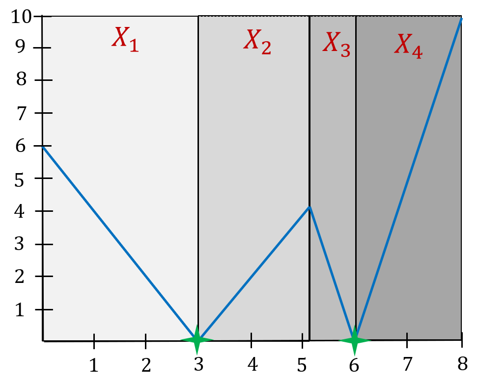
Suppose that we have a set of piecewise -log-Lipschitz functions, and consider the union over every function in this set. The following lemma states that, for every , this union contains a value such that approximates up to a multiplicative factor that depends on .
Theorem 3 (simultaneous approximation).
Let be function, where is a piecewise -log-Lipschitz function for every , and let denote the minima of as in Definition 2. Let . Then there is such that for every ,
| (4) |
Proof.
Let be the closest item to , i.e., that minimizes (Ties are broken arbitrarily). Put . We have that is a piecewise -log-Lipschitz function. Identify , let and be a partition of and a set of functions that satisfy Properties (i)–(iii) in Definition 2 for . Let such that . The rest of the proof holds by the following case analysis: (i) , (ii) and , and (iii) and . There are no other cases since if or , it will imply that or respectively, which contradicts the definition of .
Case (i) . We first prove that (4) holds for every that satisfies . If we do so, then (4) trivially holds for Case (i) by substituting since .
Let such that . Then we have
| (5) |
by the definition of and the triangle inequality. This proves (4) as
where the first and last equalities hold by the definition of , the first inequality holds since is a monotonic non-decreasing function and by (5), and the second inequality holds since is -log-Lipschitz in by Property (ii) of Definition 1.
Case (ii) and . In this case by its definition and the fact that . Hence, . Let such that . Combining the definition of with the assumption that is continuous and non-decreasing in , and is non-increasing in , we have that
| (6) |
Hence,
where the first derivation holds by combing that is non increasing in and the definition of , the second derivation is by (6), and since the last derivation holds by substituting in Case (i).
Case (iii) and . The proof for this case is symmetric to Case (ii).
Hence, in any case, there is such that for every . ∎
In what follows we define a framework for approximating general sum of functions. The goal is to minimize some loss function over a query set . This function is a function of pseudo distances, e.g. sum, max or sum of squares. A pseudo distance between an input point and a query is a Lipshitz function of their distance .
In the rest of the paper, for every minimization problem that is presented, we shall define such a cost function by specifying the functions , and , and show that we can minimize it up to some constant factor.
For example, in Section 4 we present the problem of aligning points to lines in 2 dimensional space, where the input set is a set of point-line pairs. The goal is to compute a 2D rotation matrix and a 2D translation vector that, when applied to the set of points, will minimize some cost function, for example, the sum of distances to the power of , between each point-line pair. Here, the query set is the set of all pairs of 2D rotation matrices and translation vectors , the function is the Euclidean distance between a given point-line pair after applying the transformation , i.e., , the function is , and the function simply sums those distances over all the input point-line pairs.
Definition 4 (Optimization framework).
Let be a set called ground set, be a finite input set and let be a set called a query set. Let be a function. Let be an -log-Lipschitz function and be an -log-Lipschitz function. For every we define
The following observation states that if a query approximates, up to a constant factor, the function for every input element for some other query , then also approximates up to a constant, the cost of a more involved function , relative to , where is as defined in Definition 4.
Observation 5.
Proof.
4 Algorithms for Aligning Points to Lines
In this section, we introduce our notations, describe our algorithms, and give both an overview and intuition for each algorithm. See Table I for example cost functions that our algorithms provably approximate. See Sections 4.1.2, 4.2.2 and 4.3.2 for an intuition of the algorithms presented in this section.
Notation for the rest of the paper.
Let be the set of all real matrices. We denote by the length of a point , by the Euclidean distance from to an a line in , by its projection on a set , i.e, , and by we denote the linear span of . For a matrix whose columns are mutually orthonormal, i.e., , we denote by an arbitrary matrix whose columns are mutually orthogonal unit vectors, and also orthogonal to every vector in . Hence, is an orthogonal matrix. If , we define to be the point such hat and . We denote for every integer .
For the rest of this paper, every vector is a column vector, unless stated otherwise. A matrix is called a rotation matrix if it is orthogonal and its determinant is , i.e., and . For that is called a translation vector, the pair is called an alignment. We define Alignments to be the union of all possible alignments in -dimensional space. The -axis and -axis are defined as the sets and respectively.
For a bijection (permutation) function and a set of pairs of elements, is defined as .
We use the original definition of as a set of functions and write e.g. and not to avoid dis-ambiguity as in ; see discussion in [29].
Algorithms.
We now present algorithms that compute a constant factor approximation for the problem of aligning points to lines, when the matching is either known or unknown. Algorithm 2 handles the case where the matching between the points and lines is given, i.e. given an ordered set of points, and a corresponding ordered set of lines, both in , we wish to find an alignment that minimizes, for example, the sum of distances between each point in and its corresponding line in .
Formally, let be a set of point-line pairs, , and such that is the distance between and for every and . Let be as defined in Definition 4 for . Then Algorithm 2 outputs a set of alignments that is guaranteed to contain an alignment which approximates up to a constant factor; See Theorem 9.
Algorithm 3 handles the case when the matching is unknown, i.e. given unordered sets and consisting of points and lines respectively, we wish to find a matching function and an alignment that minimize, for examples, the sum of distances between each point and its corresponding line .
4.1 Algorithm 1: Z-Configs
In this section we present a sub-routine called Z-Configs that is called from our main algorithm; see Algorithm 1 and our main algorithm in Algorithm 2.
4.1.1 Overview of Algorithm 1
The algorithm takes as input a triangle, and a line that intersects the origin. The triangle is defined by its three vertices and denoted by . The line is defined by its direction (unit vector) .
The usage of this algorithm in the main algorithm (Algorithm 2) is to compute the union over every feasible configuration , which is a rotation and a translation of such that is on the -axis, and is on the input line (simultaneously).
4.1.2 Intuition behind Algorithm 1
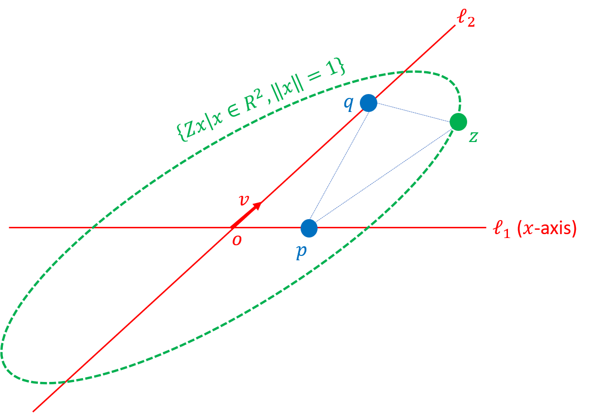
For every matrix , the set defines the boundary of an ellipse in . Hence, the shape formed by all possible locations of vertex in , assuming is on the -axis and , is an ellipse. Furthermore, this ellipse is centered around the intersection point of the -axis and (the origin, in this case). See Fig. 5.
| Input: | A unit vector such that |
| , and such that . | |
| Output: | A tuple of matrices |
| that satisfy Lemma 7. |
4.2 Algorithm 2: Align
In this section we present our main algorithm, called Align; See Algorithm 2.
| Input: | A set of pairs, |
| where for every , we have that is a point | |
| and is a line, both on the plane. | |
| Output: | A set of alignments that |
| satisfies Lemma 8. |
4.2.1 Overview of Algorithm 2
The input for Algorithm 2 is a set of pairs, each consists of a point and a line on the plane. The algorithm runs exhaustive search on all the possible tuples and outputs candidate set of alignments. Alignment consists of a rotation matrix and a translation vector . Theorem 8 proves that one of these alignments is the desired approximation.
Line 2 identifies each line by its direction (unit vector) and distance from the origin. Lines 2–2 iterates over every triple of input pairs such that , and turns it into a constant number of alignments . In Lines 2–2 we handle the case where the lines and are not parallel. In Line 2 we handle the case where and are parallel.
The case where and are not parallel. Lines 2–2 compute a rotation matrix that rotates to the -axis. Line 2 calls the sub-procedure Algorithm 1 for computing three matrices and . In Line 2 we revert the effect of the rotation matrix . Lines 2–2 compute the distance between and the intersection between and since we assumed this intersection point is the origin in Algorithm 1. The matrix and the line are used to compute a set of unit vectors in Line 2. Every defines a possible positioning for the triplet. In Line 2 we define an alignment for each . The union of the alignments in is then added to the output set in Line 2.
The case where and are parallel. In this case, we place , and place as close as possible to . If there are more than one alignment that satisfies these conditions, then we pick an arbitrary one. This is done in Line 2.
4.2.2 Intuition behind Algorithm 2
The idea behind the algorithm consists of three steps. At each step we reduce the set of feasible alignments by adding another constraint. Each constraint typically increases our approximation factor by another constant.
Consider any alignment of the input points to lines, and suppose that is the closest pair after applying this alignment. By the triangle inequality, translating the set of points so that intersects will increase the distance between every other pair by a factor of at most . Hence, minimizing (1) under the constraint that would yield a -approximation to the original (non-constrained) problem.
Similarly, we can then translate in the direction of (while maintaining ) until the closest pair, say , intersects. The result is a -approximation to the initial alignment by considering all the possible alignments of such that and . There are still infinite such alignments which satisfy the last constraint.
Hence, we add a third step. Let be the pair that requires the minimal rotation of the vector in order to minimize under the constraints that and . We now rotate the vector and translate the system to maintain the previous constraints until is minimizes.
The result is a -approximation to (1) by considering all the possible alignments of such that: is closest to among all alignments that satisfy and . Unlike the previous steps, there are only a finite number of such alignments, namely .
4.3 Algorithm 3: Alignment and Matching
4.3.1 Overview of Algorithm 3
Algorithm 3 takes as input a set of paired points and lines in , and a cost function as defined in Theorem 11. The algorithm computes an alignment and a matching function (which rearranges the given pairing of the pairs) that approximate the minimal value of the given cost function; See Theorem 11.
In Line 3 we iterate over every . In Lines 3- 3 we match to to and to , compute their corresponding set of alignments by a call to Algorithm 2, and then add to the set . Finally, in Lines 3- 3 we compute the optimal matching for every alignment in , and pick the alignment and corresponding matching that minimize the given cost function.
4.3.2 Intuition behind Algorithm 3
In Algorithm 3, we iterate over every triplet of points and triplet of lines from the input set . Each such tuple of 3 points and 3 lines define a set of alignments using Algorithm 2. For each such alignment, we compute the optimal matching function for the given cost function, using naive optimal matching algorithms. We them return the alignment and matching that yield the smallest cost.
5 Statements of Main Results
The following lemma is one of the main technical results of this paper, and lies in the heart of the proof of Lemma 8. It proves that for every two paired sets and and unit vector , there exists for some that approximates for every .
Lemma 6.
Let and . Then there is a set of unit vectors that can be computed in time such that (i) and (ii) hold as follows:
-
(i)
For every unit vector there is a vector such that for every ,
(12) -
(ii)
There is such that
Proof.
See proof of Lemma 15 in the appendix. ∎
Lemma 6 suggests a result of independent interest. Consider the constrained linear regression problem of computing a unit vector that minimizes
for a given matrix and a given vector . Lemma 6 implies that in linear time, we can compute a candidate set of unit vectors , which contains a unit vector that approximates each of the “distances” up to a multiplicative factor of . Hence, also approximates the optimal (unknown) value of the constrained linear regression , up to a multiplicative factor of . It is easy to see that a similar argument holds for the constrained regression , for , up to a constant factor that depends only on .
The following lemma proves the correctness of Algorithm 1. It proves that the matrices computed in Algorithm 1 satisfy a set of properties, which will be useful in the proof of Lemma 8.
Lemma 7.
Let be a unit vector and be the line in this direction. Let be the vertices of a triangle such that . Let be the output of a call to Z-Configs; see Algorithm 1. Then the following hold:
-
(i)
-axis and iff there is a unit vector such that and .
-
(ii)
For every unit vector , we have that if and .
Proof.
See proof of Lemma 18 in the appendix. ∎
5.1 Aligning Points-To-Lines
Table I summarizes the main results and cost functions in the context of aligning points-to-lines, which our algorithms support.
What follows is the main technical lemma for the correctness of Algorithm 2. It proves that for every (possibly optimal) alignment , the output set of Algorithm 2 must contain an alignment that approximates each of the distances for every , up to some multiplicative constant factor. Furthermore, the set is computed in time polynomial in .
Lemma 8.
Let be set of pairs, where for every , we have that is a point and is a line, both on the plane. Let be an output of a call to Align; see Algorithm 2. Then for every alignment there exists an alignment such that for every ,
| (13) |
Moreover, and can be computed in time.
Proof.
See proof of Lemma 20 in the appendix. ∎
5.1.1 Generalization
Observation 5 states that in order to approximate a complicated and non-convex cost function as in Definition 4, all needs to be done is to compute a query (alignment) that approximates the simpler (distance) function that lies in the heart of the function . Lemma 8 implies that in polynomial time we can indeed compute a query (alignment) that approximates the distance function . Combining Observation 5 with Lemma 8 yields that in polynomial time we can compute a candidates set of queries (alignments) which contain a query that approximates, up to a constant factor, a complex cost function, as follows.
Theorem 9.
Let be set of pairs, where for every , we have that is a point and is a line, both on the plane. Let and let such that is the distance between and . Let be as defined in Definition 4 for . Let if and otherwise. Let be the output of a call to Align; see Algorithm 2. Then there exists such that
Furthermore, and can be computed in time.
Proof.
See proof of Theorem 24 in the appendix. ∎
Since is guaranteed to contain an alignment that approximates the optimal value of , up to some multiplicative constant factor, simple exhaustive search in time on can find an alignment with cost smaller or equal to the cost of .
5.1.2 Unknown matching
Given an input set of unmatched pairs , an alignment (query) and some cost function, we seek a matching function , such that after rearranging the input pairs using , the rearranged (rematched) set minimizes the given cost function for the given query . A formal definition is given as follows.
Definition 10 (Optimal matching).
Let be an integer and denote the union over every permutation (bijection functions) . Let be an input set, where is a pair of elements for every , and let be a set of queries. Consider a function as defined in Definition 4 for . Let . A permutation is called an optimal matching for if it satisfies that
Recall that for and a set of pairs of elements, is defined as .
Theorem 11.
Let be a set of pairs, where for every we have that is a point and is a line, both on the plane. Let and define
for every point and line on the plane and alignment . Consider and to be as defined in Definition 4 for and . Let if and otherwise. Let be the output alignment and permutation of a call to Align+Match; see Algorithm 3. Then
| (14) |
where the minimum is over every alignment and permutation . Moreover, can be computed in time.
Proof.
See proof of Theorem 25 in the appendix. ∎
5.2 Coresets for Big Data
We now present a data reduction technique (coreset) for the points-to-lines alignment problem, based on [26]. This reduction will enable a near-linear implementation of our algorithm by running it on the small coreset while obtaining an almost similar approximation.
Theorem 12 (coreset for points-to-lines alignment).
Let be an integer. Let be set of pairs, where for every , is a point and is a line, both in , and let . Let . Then a weights vector can be computed in such that
-
(i)
With probability at least , for every it holds that
-
(ii)
The weights vector has non-zero entries.
Proof.
See proof of Theorem 31 in the appendix. ∎
Instead of running the approximation algorithms proposed in Section 4 on the entire input data, Theorem 12 implies that we can first compress the input point-line pairs in time, and then apply the approximation algorithms only on the compressed data, which will take time independent of . Hence, the total running time will be dominated by the coreset computation time. However, the approximation factor in this case will increase by an additional multiplicative factor of .
Corollary 13 (streaming, distributed, dynamic data).
Let be a (possibly infinite) stream of pairs, where for every , is a point and is a line, both in the plane. Let . Then, for every integer we can compute with probability at least an alignment that satisfies
for the points seen so far in the stream, using memory and update time per a new pair. Using machines the update time can be reduced by a factor of .
Proof.
See proof of Corollary 32 in the appendix. ∎
6 Conclusion and Open Problems
We described a general framework for approximating functions under different constraints, and used it for obtaining generic algorithms for minimizing a finite set of piecewise log-Lipschitz functions. We apply this framework to the points-to-lines alignment problem. Coresets for these problems enabled us to turn our polynomial time algorithms in some cases into near linear time, and support streaming and distributed versions for Big Data.
Open problems include generalization of our results to higher dimensions, as some of our suggested coresets. We generalize our algorithms for the case when no matching permutation is given between the points and lines. However, the results are less general than our results for the known matching case, and we do not have coresets for these cases, which we leave for future research.
References
- [1] G. K. Tam, Z.-Q. Cheng, Y.-K. Lai, F. C. Langbein, Y. Liu, D. Marshall, R. R. Martin, X.-F. Sun, and P. L. Rosin, “Registration of 3d point clouds and meshes: a survey from rigid to nonrigid,” IEEE transactions on visualization and computer graphics, vol. 19, no. 7, pp. 1199–1217, 2013.
- [2] M. Fischler and R. Bolles, “Random sample consensus: a paradigm for model fitting with applications to image analysis and automated cartography,” Communications of the ACM, vol. 24, no. 6, pp. 381–395, 1981.
- [3] I. Jubran and D. Feldman, “Demonstration of our algorithms in a real-time system. link: {https://drive.google.com/open?id=19I6Jd6F8ET9386yahKx3Dgr6gBTuzYhJ}.”
- [4] P. J. Huber, Robust statistics. Springer, 2011.
- [5] P. Agarwal, S. Har-Peled, and K. Varadarajan, “Approximating extent measures of points,” Journal of the ACM, vol. 51, no. 4, pp. 606–635, 2004.
- [6] D. Feldman and T. Tassa, “More constraints, smaller coresets: Constrained matrix approximation of sparse big data,” in KDD. ACM, 2015, pp. 249–258.
- [7] K. Derpanis, “Overview of the ransac algorithm,” Image Rochester NY, vol. 4, no. 1, pp. 2–3, 2010.
- [8] P. Besl and N. McKay, “Method for registration of 3-d shapes,” in Control Paradigms and Data Structures, vol. 1611. Intl. Society Optics & Photonics, 1992, pp. 586–607.
- [9] D. Feldman and M. Langberg, “A unified framework for approximating and clustering data,” in STOC, 2011, pp. 569–578, see http://arxiv.org/abs/1106.1379 for fuller version.
- [10] D. Feldman, A. Fiat, M. Sharir, and D. Segev, “Bi-criteria linear-time approximations for generalized k-mean/median/center,” in SoCG. ACM, 2007, pp. 19–26.
- [11] A. Vigneron, “Geometric optimization and sums of algebraic functions,” ACM Transactions on Algorithms (TALG), vol. 10, no. 1, p. 4, 2014.
- [12] B. Chazelle, H. Edelsbrunner, L. J. Guibas, and M. Sharir, “A singly exponential stratification scheme for real semi-algebraic varieties and its applications,” Theoretical Computer Science, vol. 84, no. 1, pp. 77–105, 1991.
- [13] D. Y. Grigor’Ev and N. N. Vorobjov Jr, “Solving systems of polynomial inequalities in subexponential time,” Journal of symbolic computation, vol. 5, no. 1-2, pp. 37–64, 1988.
- [14] M. Frank and P. Wolfe, “An algorithm for quadratic programming,” Naval research logistics quarterly, vol. 3, no. 1-2, pp. 95–110, 1956.
- [15] C. R.S., D. Feldman, and D. Rus, “Trajectory clustering for motion prediction,” in IROS’12, 2012, pp. 1547–1552.
- [16] R. P., D. F., D. R., and P. N., “Visual precis generation using coresets,” in ICRA’14, 2014, pp. 1304–1311.
- [17] D. D. Needelman, R. Li, and Y.-W. A. Wu, “Refinement of spacecraft angular velocity and attitude estimates using star data,” Jun. 13 2006, uS Patent 7,062,363.
- [18] G. M. and D. P., “Uncalibrated video compass,” in 2007 RSS, 2007, pp. 226–231.
- [19] S. Hijikata, K. Terabayashi, and K. Umeda, “A simple indoor self-localization system using infrared leds,” in INSS’09. IEEE, 2009, pp. 1–7.
- [20] K. Geisner, B. Mount et al., “Realistic occlusion for a head mounted augmented reality display,” Sep. 1 2015, uS Patent 9,122,053.
- [21] S. Li, C. Xu, and M. Xie, “A robust o (n) solution to the perspective-n-point problem,” IEEE transactions on pattern analysis and machine intelligence, vol. 34, no. 7, pp. 1444–1450, 2012.
- [22] V. Lepetit, F. Moreno-Noguer, and P. Fua, “Epnp: An accurate o (n) solution to the pnp problem,” International journal of computer vision, vol. 81, no. 2, p. 155, 2009.
- [23] Y. Zheng, Y. Kuang, S. Sugimoto, K. Astrom, and M. Okutomi, “Revisiting the pnp problem: A fast, general and optimal solution,” in Proceedings of the IEEE International Conference on Computer Vision, 2013, pp. 2344–2351.
- [24] P. Wang, G. Xu, Y. Cheng, and Q. Yu, “A simple, robust and fast method for the perspective-n-point problem,” Pattern Recognition Letters, vol. 108, pp. 31–37, 2018.
- [25] S. Urban, J. Leitloff, and S. Hinz, “Mlpnp-a real-time maximum likelihood solution to the perspective-n-point problem,” arXiv preprint arXiv:1607.08112, 2016.
- [26] A. Dasgupta, P. Drineas, B. Harb, R. Kumar, and M. Mahoney, “Sampling algorithms and coresets for regression,” SIAM Journal on Computing, vol. 38, no. 5, pp. 2060–2078, 2009.
- [27] M. B. Cohen and R. Peng, “L p row sampling by lewis weights,” in Proceedings of the forty-seventh annual ACM symposium on Theory of computing. ACM, 2015, pp. 183–192.
- [28] D. Feldman and L. Schulman, “Data reduction for weighted and outlier-resistant clustering,” in SODA. SIAM, 2012, pp. 1343–1354.
- [29] R. Graham, D. Knuth, O. Patashnik, and S. Liu, “Concrete mathematics: a foundation for computer science,” Computers in Physics, vol. 3, no. 5, pp. 106–107, 1989.
- [30] H. W. Kuhn, “The hungarian method for the assignment problem,” Naval Research Logistics (NRL), vol. 2, no. 1-2, pp. 83–97, 1955.
- [31] V. Braverman, D. Feldman, and H. Lang, “New frameworks for offline and streaming coreset constructions,” arXiv preprint arXiv:1612.00889, 2016.
- [32] M. Anthony and P. L. Bartlett, Neural network learning: Theoretical foundations. cambridge university press, 2009.
- [33] D. Feldman, M. Schmidt, and C. Sohler, “Turning Big Data into Tiny Data: Constant-size Coresets for k-means, PCA and Projective Clustering,” in Proceedings of the 24th ACM-SIAM Symposium on Discrete Algorithms (SODA), 2013, pp. 1434 – 1453.
- [34] J. L. Bentley and J. B. Saxe, “Decomposable searching problems i. static-to-dynamic transformation,” Journal of Algorithms, vol. 1, no. 4, pp. 301–358, 1980.
- [35] A. Barger and D. Feldman, “k-means for streaming and distributed big sparse data,” in SDM. SIAM, 2016, pp. 342–350.
- [36] I. Jubran and D. Feldman, “Open source code for all the algorithms and experimental results in this paper,” 2018, the authors commit to publish upon acceptance of this paper or reviewer request.
- [37] R. Raguram, J. Frahm, and M. Pollefeys, “A comparative analysis of ransac techniques leading to adaptive real-time random sample consensus,” in ECCV, 2008, pp. 500–513.
- [38] H. Bay, T. Tuytelaars, and L. Van Gool, “Surf: Speeded up robust features,” in European conference on computer vision. Springer, 2006, pp. 404–417.
- [39] B. D. Lucas, T. Kanade et al., “An iterative image registration technique with an application to stereo vision,” 1981.
- [40] R. O. Duda and P. E. Hart, “Use of the hough transformation to detect lines and curves in pictures,” Communications of the ACM, vol. 15, no. 1, pp. 11–15, 1972.
- [41] E. Marchand, H. Uchiyama, and F. Spindler, “Pose estimation for augmented reality,” IEEE transactions on visualization and computer graphics, vol. 22, no. 12, pp. 2633–2651, 2016.
Appendix A Proofs of Main Results
In this section we first present and prove helpful lemmas, and then present the main results and their proofs
The following lemma states that if a function is concave in an interval that contains , then is -log-Lipschitz.
Lemma 14.
Let be an interval that contains , and let such that the second derivative of is defined and satisfies for every . Then is -log-Lipschitz in , i.e., for every and , it holds that
Proof.
Since for every , we have that is concave in the interval . Therefore, for every , it holds that
| (15) |
Let and put . By substituting and in (15), we have
Rearranging terms yields
| (16) |
where the second derivation is since by the definition of . Hence, it holds that
where the first inequality holds by substituting and in (15), and the second inequality holds by (16). ∎
Lemma 15 (Lemma 6).
Let and . Then there is a set of unit vectors in that can be computed in time such that (i) and (ii) hold as follows:
-
(i)
For every unit vector there is a vector such that for every ,
(17) -
(ii)
There is such that
Proof.
Proof of (i): By Theorem 3 it suffices to prove that is piecewise -log-Lipschitz over every unit vector , and then define to include all the minima of , over every . The proof that is piecewise -log-Lipschitz for is based on the case analysis of whether or in Claims 16 and 17 respectively. The proofs of these cases use Lemma 14.
Indeed, let , such that , and let be an interval. Here we assume , otherwise (17) trivially holds for . For every , let
and let . Hence, for every ,
| (18) |
Claim 16.
If then is piecewise -log-Lipschitz.
Proof.
Suppose that indeed . In this case, for every , so the absolute value in can be removed, i.e., for every ,
Let and let such that
Since for every , we have
| (19) |
We now prove that is -log-Lipschitz for every . For every we have
| (20) |
where the first equality holds by the definition of and the second equality holds since for every .
By taking the square of the last inequality, it holds that for every ,
| (21) |
Thus, for every , it holds that
| (22) |
where the first and last equalities are by (20), the first inequality is by combining and (21), and the second inequality holds since . By Definition 1, it follows that is -log-Lipschitz for every .
By substituting in Definition 2 and for every , Properties (i)-(iii) of Definition 2 hold for since
Hence, is a piecewise -log-Lipschitz function.
∎
Claim 17.
If then is piecewise -log-Lipschitz.
Proof.
Let
and let
First, observe that . Second, for every ,
Let . We now prove that is piecewise -log-Lipschitz for every by proving that
(i): is -log-Lipschitz in , i.e., for every .
(ii): is -log-Lipschitz in , i.e., for every .
Since and for every , we conclude by (ii) that is -log-Lipschitz in , i.e., for every .
Since and for every , we conclude by (i) that is -log-Lipschitz in , i.e., for every .
The proof of (i) and (ii) above is as follows.
Proof of (i): Clearly, if , (i) trivially holds as
| (23) |
Let such that . The denominator is positive since in the range of .
We first prove that does not get its maximum at . Observe that
| (24) |
where the second derivation holds since , and the last derivation holds since .
Since , we have by (24) that . Hence, is decreasing in the neighbourhood of . Therefore, is not an extreme point of .
We now prove that for . Suppose that maximizes over the open interval . Since is continuous in an open interval, the derivation of at is zero, i.e.,
We also have that since
Hence,
| (25) |
For every , let . Observe that for every . Substituting and in Lemma 14 yields
| (26) |
Hence, for every it follows that
| (27) |
where the first derivation is by the definition of , the second derivation is by (25) and the last derivation is by substituting in (26). We also have that
| (28) |
where the second equality holds by L’hospital’s rule since for .
By combining (24), (27) and (28), we get that for every . By combining (23) with the last inequality, (i) holds as for every .
Proof of (ii): We have that for . Since for every , by substituting and in Lemma 14, (ii) holds as
| (29) |
for every .
By (i) and (ii) we can now prove the lemma as follows. Observe that and are the minima of over when . By Definition 2 we have that is piecewise -log-Lipschitz function in since
-
1.
has a unique infimum in , is -log-Lipschitz in , and for every .
-
2.
has a unique minimum in , is -log-Lipschitz in , and for every .
-
3.
has a unique infimum in , is -log-Lipschitz in , and for every .
-
4.
has a unique minimum in , is -log-Lipschitz in , and for every .
∎
Recall that . Since , by Claims 16 and 17 it holds that is piecewise -log-Lipschitz function for every .
Hence, by substituting in Theorem 3 with , and , there exists a minimum such that for every ,
| (30) |
Let be a unit vector, such that , , and let be the index such that . Hence,
where the first equality holds by the definition of , the second and fourth equalities holds by (18), the inequality holds by (30), and the last equality holds since .
Proof of Lemma 15 (ii): The proof follows immediately by the definition of in (i).
Observe that it takes time to compute for a fixed . Hence, Lemma 15 holds by letting , since it takes time to compute . ∎
A.1 Aligning Points-To-Lines
Lemma 18 (Lemma 7).
Let be a unit vector such that and be the line in this direction. Let be the vertices of a triangle such that . Let be the output of a call to Z-Configs; see Algorithm 1. Then the following hold:
-
(i)
We have both -axis and if and only if there is a unit vector such that and .
-
(ii)
For every unit vector , we have that if and .
Proof.
We use the variables that are defined in Algorithm 1.
(i) : Let and such that and . We need to prove that -axis and . Indeed,
where the first equality holds since the vector is orthogonal to the -axis and the last equality holds since by the definition of in Line 1 of Algorithm 1. Hence, -axis. Let . We also have
where the third equality holds by the definition of , and the fourth equality holds since . Hence, .
(i) : Let -axis and . We need to prove that there exists a unit vector such that and . Let such that , and be a triangle, where is the origin of . Let be the interior angle at vertex and let be the angle at vertex of the triangle . Observe that the sin of the angle at vertex is simply . Let . By simple trigonometric identities in the triangle , we have
| (31) |
We continue with the following case analysis: (a): , (b): and (c): .
Case (a) : By the law of sines we have that . Let . Hence, respectively,
| (32) |
and
| (33) |
Then it holds that
| (34) |
where the third equality holds by combining (32) with the definition , and the last equality holds by the definition of . It also holds that
| (41) | ||||
| (46) | ||||
| (49) |
where the two equalities in (46) hold respectively by the definition and by (31), and the two equalities in (49) hold by (33) and the definition of respectively. Combining (34) and (49) yields that the vector satisfies and .
Case (b) : In this case, since , it holds that intersects the origin , i.e., , and since . Then by setting respectively, it holds that, and . Hence, there exists a unit vector such that and .
Case (c) : In this case, since , it holds that intersects the origin , i.e., . Similarly to (34), it holds that for . It also holds that
| (56) | ||||
| (61) |
where the fourth equality holds by combining (31) and . Hence, there exists a unit vector such that and
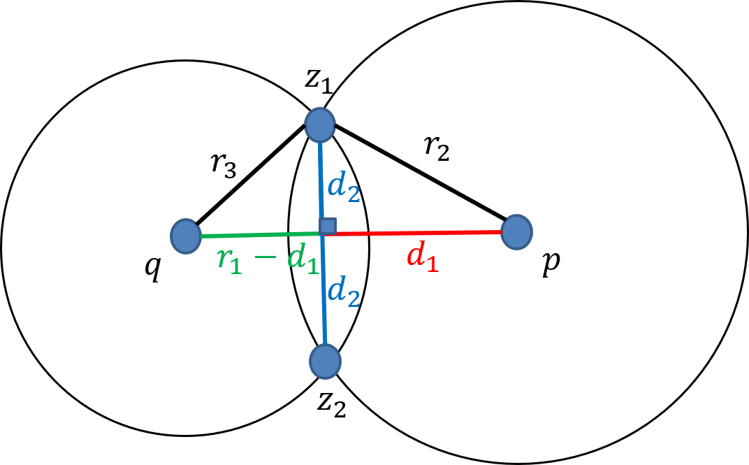
(ii): Suppose that and for some unit vector . By (i) we have that -axis and . We need to prove that . Consider the triangle . Vertex lies at one of the intersection points of the pair of circles whose radii are , centered at and , respectively; See Fig. 6. The position of is given by
| (62) |
where is or if lies respectively in the halfplane to the right of the vector or otherwise. If lies exactly on the line spanned by the vector , then can take either or since, in that case, ; See illustration in Fig 6. The first equality in (62) holds since the vector and are an orthogonal basis of , and the last equality holds since is a radian counter clockwise rotation matrix, i.e., for every vector it satisfies that . Substituting and in (62) proves Claim (ii) as
∎
Corollary 19.
Let be a line on the plane that intersects the origin and is spanned by the unit vector . Let such that is on the -axis, is on line and . For every , let denote the output of a call to Z-Configs; see Algorithm 1. Then (i) and (ii) holds as follows.
-
(i)
There is a unit vector such that for every we have .
-
(ii)
For every unit vector , there is a corresponding alignment , such that for every .
Proof.
(i): By Lemma 18 (i), since -axis and , there is a unit vector such that and . By Lemma 18 (ii), since and , we have for every . Hence, there is a unit vector such that for every .
(ii): Let be a unit vector. Since for every unit vector , there is an aligning that aligns the points and with the points and , i.e., and . Let . Consider the triangle after applying the alignment to triangle . Hence, , and . By the definition of , we also have and . By Lemma 18 (ii), the unit vector satisfies . Hence, . ∎
The proof of the following lemma is divided into 3 steps that correspond to the steps discussed in the intuition for Algorithm 2 in Section 4.2.2.
Lemma 20 (Lemma 8).
Let be a set of pairs, where for every , we have that is a point and is a line, both on the plane. Let be an output of a call to Align; see Algorithm 2. Then for every alignment there exists an alignment such that for every ,
| (63) |
Moreover, and can be computed in time.
Proof.
Let . Without loss of generality, assume that the set is already aligned by , i.e., and .
Step 1. We first prove that there is , such that translating until it intersects does not increase the distance by more than a multiplicative factor of , for every . See Fig. 7.
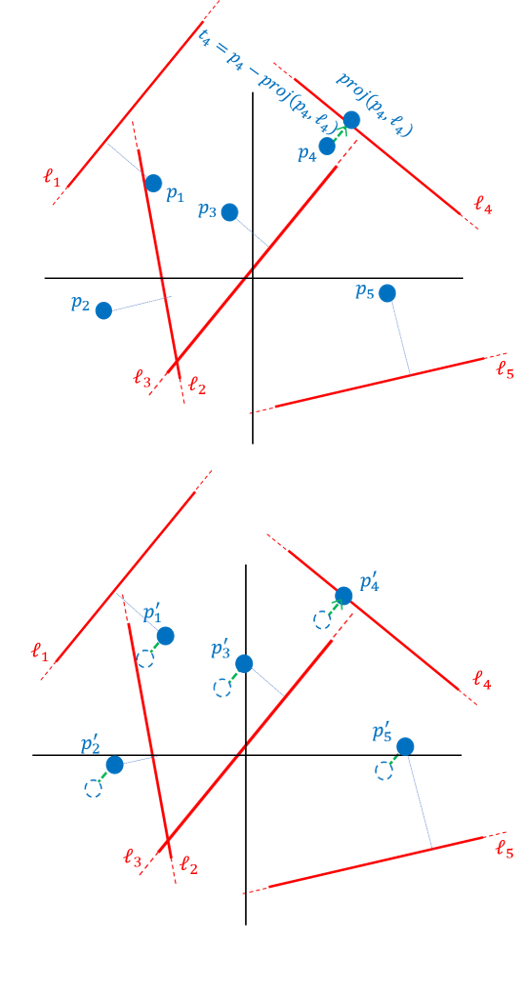
Put . Let and let . Hence,
| (64) | ||||
| (65) | ||||
| (66) |
where (64) holds due to the triangle inequality, (65) holds due to the definition of , and (66) holds since . For every , let and without loss of generality assume that is the origin, otherwise translate the coordinate system.
Let be a unit vector and such that
In what follows we assume that cannot all be mutually parallel, i.e., there exists at least two lines that intersect. We address the case where all the lines are parallel in Claim 23.
Step 2. We prove in Claim 21 that there is such that translating in the direction of , until it gets as close as possible to will not increase the distance by more than a multiplicative factor of . See Fig. 8.
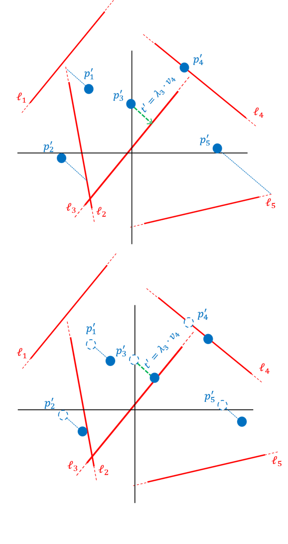
Let and set
Informally, if and only if and are parallel lines, and it represents the distance that needs to travel in the direction parallel to until it intersects . Observe that there is at least one index such that since we assumed the lines are not all mutually parallel.
Claim 21.
There exists and a corresponding translation vector such that for every ,
Proof.
Let . Put . Let . Observe that is a line in . If is parallel to , then since both and are on , the claim trivially holds as
We now assume that and are not parallel. Let be the angle between and , and let . Observe that
| (67) |
and that for every ,
| (68) |
Then the claim holds as
| (69) | ||||
| (70) | ||||
| (71) | ||||
| (72) | ||||
| (73) |
where (69) holds by substituting in (68), (70) holds by the triangle inequality, (71) since , (72) holds by combining the definition of with (67), and (73) holds by substituting in (68). ∎
Let and be respectively the index and the translation vector that are computed in Claim 21. For every , let denote the point after translation by , i.e., .
Since is the index corresponding to the minimal , we have that (since there is at least one such ). By the definitions of for every , we have that only if and are not parallel. Combining the two previous facts yields that and are not parallel. Furthermore, since we defined to be exactly the translation distance in the direction of needed for to intersect , we have that .
Step 3. In the following claim we prove that there is an alignment that satisfies the following: (i) and , (ii) minimizes the distance for some index over every that satisfy and , and (iii) satisfies for every .
Claim 22.
Let . Then there exists and an alignment such that for every ,
Proof.
Put . We have that since is assumed to be the origin in Step 1, and by the definition . Let be a rotation matrix that aligns with the -axis, i.e., . By substituting and in Lemma 7 (i) and (ii) (where and are rotated together such that is the origin), we have that there is a unit vector and matrices and such that and . The matrices and are multiplied by the inverse rotation matrix to simulate the inverse rotation which was applied on and before applying Lemma 7. Observe that
| (74) |
where the second equality holds since . By substituting in Lemma 15 (i), there is a set of unit vectors, and an index , such that for every unit vector
| (75) |
Substituting and in Corollary 19 (ii) implies that there is an alignment that aligns the set with the set , i.e. . Hence, the following holds
| (76) | ||||
| (77) | ||||
| (78) | ||||
| (79) |
where (76) holds since , (77) holds since , (78) holds by (75) and (79) holds by (74).
Hence, by Step 1, there exists an alignment that aligns a point with for some , and does not increase the distances of the other pairs by more than a multiplicative factor of . This is the reason that all the output alignments of Algorithm 2 satisfy that one of the input points intersects its corresponding line.
By the proof in Step 2, there exists an alignment that aligns a point with for some , and does not increase the distances of the other pairs by more than a multiplicative factor of . This is the reason that all the output alignments of Algorithm 2 satisfy that two of the input points intersect their corresponding lines, if the input lines are not all mutually parallel.
By the proof in Step 3, there exists an alignment that minimizes the distance between and for some , and maintains that and . This alignment provably guarantees that the distance of the other pairs does not increase by more than a multiplicative factor of .
Hence, if the input lines are not all mutually parallel, we proved there are where , and , such that the following is satisfied
| (80) |
So far we have proven Step 1 regardless of weather the lines are mutually parallel or not. However, we proved Step 2 and step 3 (Claims 21 and 22 respectively) of Lemma 20 only for the case that the lines are not all mutually parallel. We now prove an alternative claim (Claim 23) instead of Claims 21 and 22 for the case that are mutually parallel.
Recall that . By Step 1, we have that . To handle the case where all the lines are parallel, we now prove that rotating the points around until the distance for some is minimized would increase the distance for every by a factor of at most .
Claim 23.
If are mutually parallel, then there exists and a rotation matrix
where the minimum is over every rotation matrix , such that for every ,
Proof.
Let be an arbitrary (known) unit vector. Let be a rotation matrix that rotates to the direction of , i.e., , and define . Therefore
| (81) |
By Lemma 15(i), there is a set of unit vectors and , such that
| (82) |
Let be the index from Lemma 15(ii). Define to be the rotation matrix that satisfies . Hence,
| (83) | ||||
| (84) | ||||
| (85) | ||||
| (86) | ||||
| (87) | ||||
| (88) |
where (83) holds by the definition of , (84) holds since the rotation matrix group is commutative, (85) holds by the definition of , (86) holds by the definition of , (87) holds by (82) and (88) holds by (81).
By the definition of and , it follows that minimizes . Similarly to (86), it holds that , so . Hence, and satisfy the requirements of this Claim. ∎
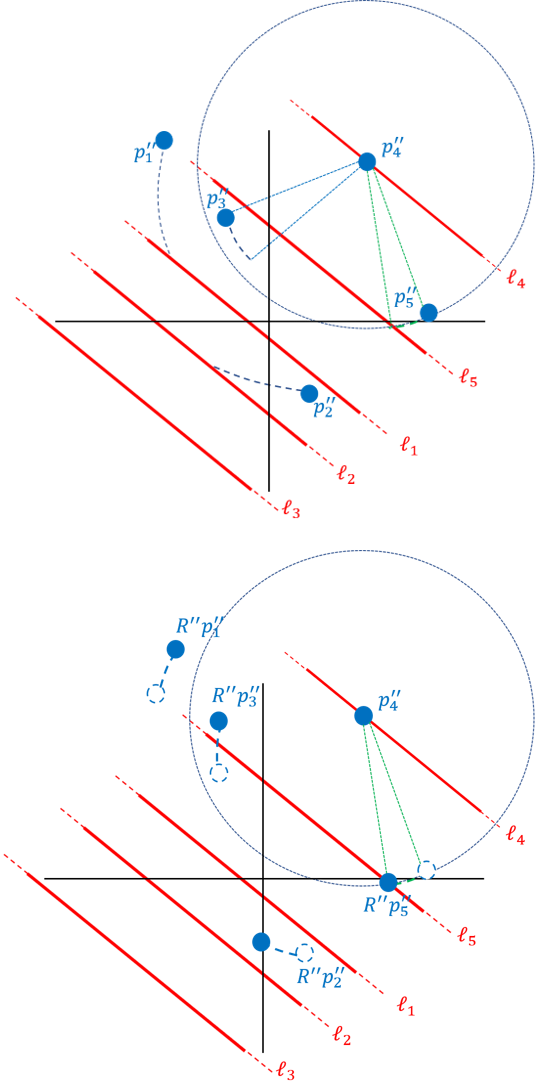
Hence, by Step 1 and Claim 23, if all the lines are parallel, there are , where , and , such that the following holds
| (89) |
Algorithm 2 iterates over every triplet . There are such triplets. The alignments that satisfy (80) are computed in Lines 2 2 and stored in . The alignments that satisfy 89 are computed in Line 2 and stored in . The sets and computed at every iteration are of constant size, i.e., . We output , the union of all those alignments. Hence, will contain an alignment that satisfies (63), and . Furthermore, the running time of Algorithm 2 is since Lines 2- 2 take time to compute, and are executed times. ∎
Theorem 24 (Theorem 9).
Let be set of pairs, where for every , we have that is a point and is a line, both on the plane. Let and let such that is the norm between and . Let be as defined in Definition 4 for . Let if and otherwise. Let be the output of a call to Align; see Algorithm 2. Then there exists such that
Furthermore, and can be computed in time.
Proof.
By (90) and since the -norm of every vector in is approximated up to a multiplicative factor of (as defined in the theorem) by its -norm, we obtain that
By substituting and in Observation 5, Theorem 24 holds as
where the last derivation holds by the definition of .
Furthermore, it takes time to compute . ∎
Theorem 25 (Theorem 11).
Let be a set of pairs, where for every we have that is a point and is a line, both on the plane. Let and for every point and line on the plane and alignment . Consider to be a function as defined in Definition 4 for and . Let if . Otherwise, . Let be the output alignment and permutation of a call to Align+Match; see Algorithm 3. Then
| (91) |
where the minimum is over every alignment and permutation .
Moreover, can be computed in time.
Proof.
Let . By Theorem 24, we can compute a set such that there exists an alignment that satisfies
| (92) |
where is computed by a call to Align; see Algorithm 2.
In Line 2 of Algorithm 2 we iterate over every triplet of indices . Each such index corresponds to a point-line matched pair. Hence, and correspond to a triplet of matched point-line pairs. In Lines 2, we add alignments to the set that correspond to that triplet of point-line pairs. Therefore, every alignment corresponds to some 3 matched point-line pairs . Let be the triplet of matched pairs that corresponds to the alignment . Hence, it holds that
By iterating over every and , when and , we get that
In Line 3 of Algorithm 3 we iterate over every tuple of 6 indices , and compute, using Algorithm 2, the set of alignments that corresponds to the triplet of pairs . We then add those alignments to the set . Hence, it is guaranteed that the alignment that satisfies (92) is also in .
The bijection (matching) function that minimizes the sum of distances (or in some other cost function) between the point and the line over can be computed in time as explained in [30]. We use this algorithm to compute the optimal matching function for every in Line 3 of Algorithm 3. Let . Since is an optimal matching function for the pairs of , the alignment , and the function , it satisfies that
| (93) |
Since and , we obtain that , where is the set that is defined in Line 3 of Algorithm 3. Combining with the definition of in Line 3, it yields
| (94) |
Appendix B Coresets for Big Data
The following theorem states Theorem 4 from [26] for the case where .
Theorem 26 (Theorem 4 in [26]).
Let be an matrix of rank . Then there exists an matrix that satisfies the following
-
(i)
is a basis for the column space of , i.e., there exists a matrix such that .
-
(ii)
.
-
(iii)
For every , .
-
(iv)
can be computed in time.
Lemma 27.
Let , where for every . Then a function
can be computed in time such that
-
(i)
For every ,
-
(ii)
Proof.
Let denote the rank of .
(i): By substituting in Theorem 26, we get that there exists a matrix and a matrix with the following properties:
Let be the th row of for .
Observe that for every such that , we have that
| (95) |
where the second derivation holds since is a unit vector, and the last derivation holds since . Let such that . Then it follows that
| (96) |
where the first derivation holds by combining Property (1) and the definition of , the second derivation holds by substituting in Property (3), and the fourth derivation holds by substituting and in (95). Let be the pseudo inverse of . It thus holds that is the identity matrix. Hence
| (97) |
where is the th column of the identity matrix. By combining (96) and (97), we have
| (98) |
Let
By combining the definition of and that (98) holds for every , Property (i) of Lemma 27 holds as
Furthermore, the time needed to compute is dominated by the computation time of and , which is bounded by due to Property (4). ∎
Definition 28 (Definition 4.2 in [31]).
Let be a finite set, and let . Let be a function that maps every set to a corresponding set , such that for every . Let be a cost function. The tuple is called a query space.
Definition 29 (VC-dimension).
For a query space , and we define
and
The dimension of the query space is the -dimension of .
Theorem 30 (Theorem 5.5 in [31]).
Let be a query space; see Definition 28. Let such that
for every such that the denominator is non-zero. Let and Let be the dimension of query space . Let be a sufficiently large constant and let . Let be a random sample of
points from , such that is sampled with probability for every . Let for every . Then, with probability at least , for every it holds that
Theorem 31 (Theorem 12).
Let be an integer. Let be set of pairs, where for every , is a point and is a line, both in , and let . Let . Then in time we can compute a weights vector that satisfies the following pair of properties.
-
(i)
With probability at least , for every it holds that
-
(ii)
The weights vector has non-zero entries.
Proof.
Put . We represent a line by a basis of its orthogonal complement and its translation from the origin. Formally, let be a matrix whose rows are mutually orthogonal unit vectors, and such that
Identify the rows of by , and let
Let , and for every let
where the th row of is Then it holds that
| (99) | |||
| (100) |
where (99) holds by the definition of and (100) holds by the definition of for every . Hence,
| (101) |
We have for every . Plugging this in (101) yields
| (102) |
For every and , let and such that , and let . Similarly to (102), for every ,
| (103) |
Let
and let
Then the following holds
| (104) | |||
| (105) | |||
| (106) | |||
| (107) | |||
| (108) | |||
| (109) |
where the supremum is over every alignment such that , and where (105) holds by 103, (106) holds by the definition of , (106) holds since the maximum of a sum is at most the sum of maxima, and (109) holds since .
Therefore,
| (110) |
By substituting in Lemma 27, we get that in time we can compute a function that maps every column of to a non-negative real such that the following two properties hold for every and :
| (111) |
| (112) |
Let such that for every . Then we have
| (113) |
where the first derivation holds by (111), and the last is by the definition of .
We also have that
| (114) |
where the first derivation is by the definition of and the third derivation is by (112).
The dimension of the corresponding query space is bounded by by [32].
Let . Let be a random sample of
pairs from , where is sampled with probability and let where
for every . By substituting , , for every , , and , in Theorem 30, Property (i) of Theorem 12 holds as
Furthermore, Property (i) of Theorem 31 holds since the number of non-zero entries of is equal to .
The time needed to compute is bounded by the computation time of , which is bounded by . ∎
Corollary 32 (Corollary 13).
Let be a (possibly infinite) stream of pairs, where for every , is a point and is a line, both in the plane. Let . Then, for every integer we can compute with probability at least an alignment that satisfies
for the points seen so far in the stream, using memory and update time per a new pair. Using machines the update time can be reduced by a factor of .
Proof.
B.1 Experimental Results
The main contribution of this paper is the theorems and theoretical results in previous sections. Nevertheless, since the algorithms are relatively simple we were able to implement them in an open source library [36] in order to demonstrate their correctness and robustness. In this section we suggest preliminary experimental results on synthetic and real data, and some comparison to existing software.
Hardware.
All the following tests were conducted using MATLAB R2016b on a Lenovo Y700 laptop with an Intel i7-6700HQ CPU and 16GB RAM.
B.1.1 Synthetic Data
The input data-set
was generated by first computing a set of random lines in the plane. then, a set of random points was generated, each in the range . A set was then computed by projecting the th point of the points in onto its corresponding line in . The set was then translated and rotated, respectively, by a random rotation matrix and a translation vector to obtain a set . Then, a random noise was added for every point , and additional noise was added to a subset of points (outliers), where is the percentage of outliers. The resulting set was denoted by .
The randomness in the previous paragraph is defined as follows. Let denote a Gaussian distribution with mean and standard deviation . Similarly, let denote uniform distribution over . For every and , the line was constructed such that and . For every , we choose , , and . The rotation matrix was chosen such that and .
Experiment.
The goal of each algorithm in the experiment was to compute and , approximated rotation and translation , respectively, using only the set of lines and the corresponding noisy set of points. Two tests were conducted, one with a constant number of input points , with increasing percentage of outliers, and another test with a constant value for , while increasing the number of input points. For the first test we compare the threshold M-estimator of the sum of fitting distances
| (115) |
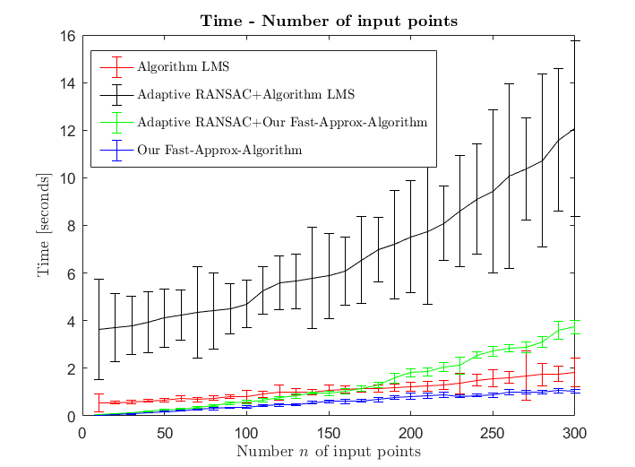
For the second test we compare the running time (in second) of the suggested methods.
Algorithms.
We apply each of the following algorithms that gets the pair of sets and as input.
Our Fast-Approx-Alignment samples a set of points from . Let be lines in corresponding to the points in . It then runs Algorithm 2 with the set of corresponding point-line pairs from and . The algorithm returns a set of alignments. We then chose the alignment that minimizes Eq. (115) using .
Algorithm LMS returns an alignment that minimizes the sum of squared fitting distances (Least Mean Squared), i.e., , where the minimum is over every valid alignment . This is done by solving the set of polynomials induced by the sum of squared fitting distances function using the Lagrange Multipliers method.
Adaptive RANSAC + Algorithm LMS is an iterative method that uses iterations, proportional to the (unknown) percentage of outliers. See [37]. At the iteration it samples 3 pairs of corresponding points and lines from and , respectively, it then computes their optimal alignment using Algorithm LMS , and then updates the percentage of inliers found based on the current alignment. A point is defined as an inlier in the iteration if , where . It then picks the alignment that has the maximum number of inliers over every alignment in .
Adaptive RANSAC + our Fast-Approx-Alignment similar to the previous Adaptive RANSAC Algorithm, but instead of using Algorithm LMS , it uses our Fast-Approx-Alignment to compute the alignment of the triplet of pairs at each iteration.
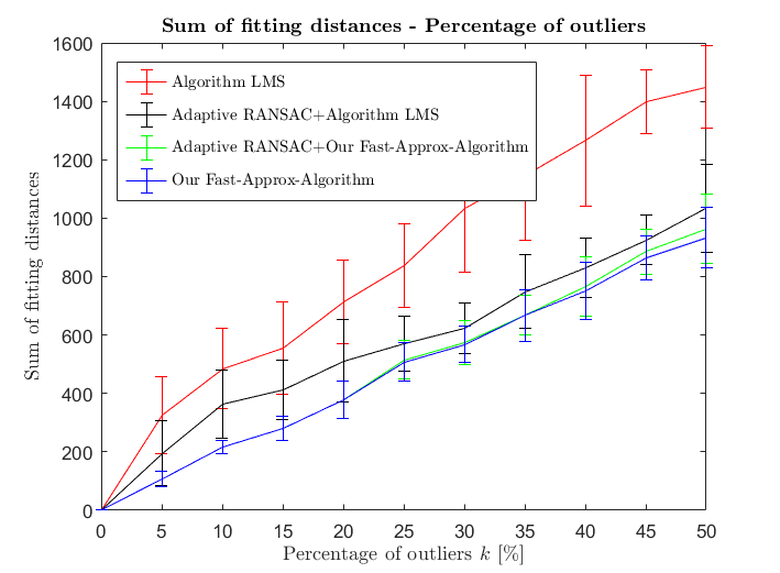
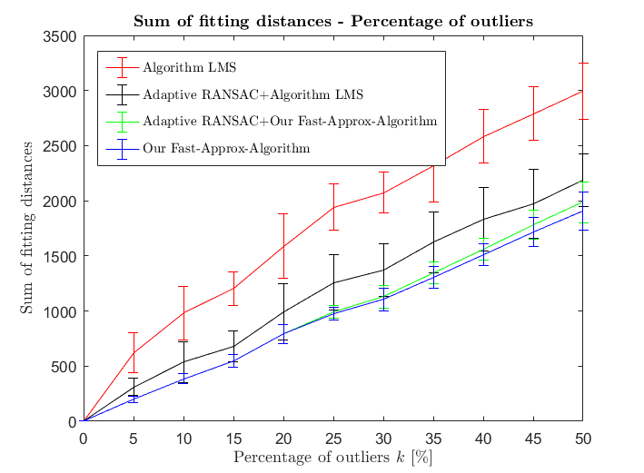
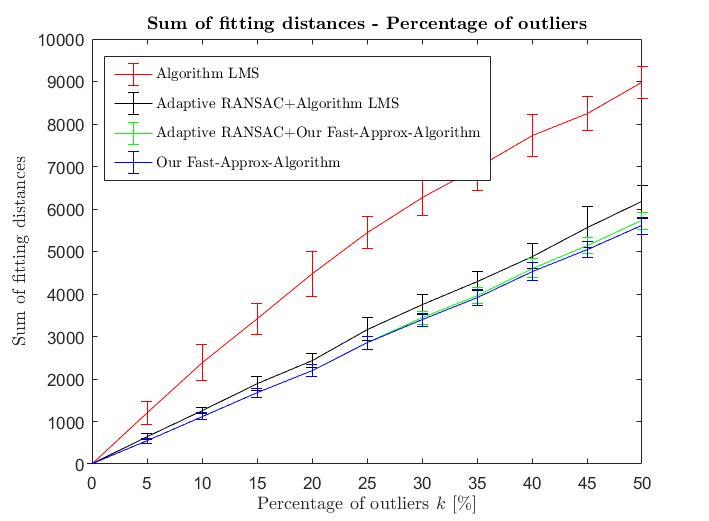
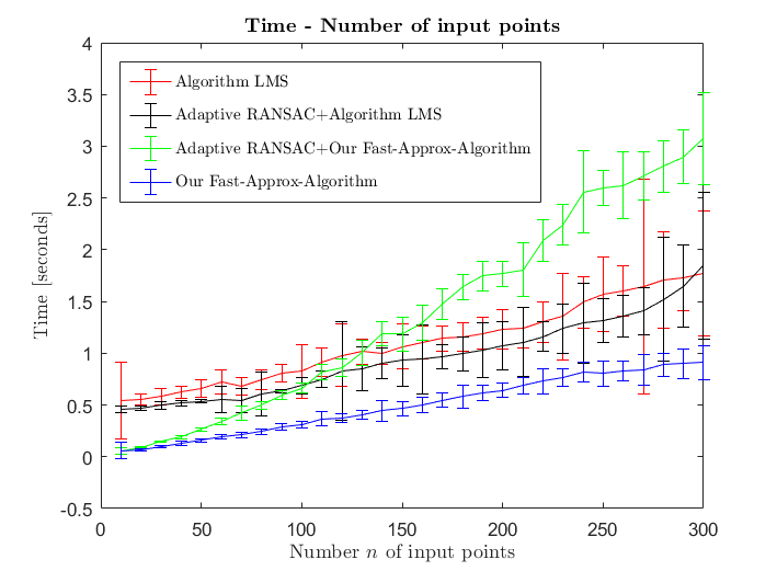
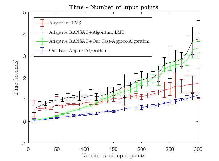
Each test was conducted times. The average sum of fitting distances, along with the standard deviation are shown in Fig. 10(a), Fig. 10(b) and Fig. 10(c). The average running times, along with the standard deviation, are shown in Fig. 11(a), Fig. 11(b) and Fig. 11(c).
B.1.2 Real Data
We have conducted a test with real-world data to emphasize the potential use of our algorithm in real-world applications; See video in [3] or in the supplementary material.
Experiment: Potential application for Augmented Reality.
A small camera was mounted on a pair glasses. The glasses were worn by a person (me), while observing the scene in front of him, as shown in Fig 3. The goal was to insert 2D virtual objects into the video of the observed scene, while keeping them aligned with the original objects in the scene.
The experiment.
At the first frame of the video we detect a set of ”interesting points” (features) using a SURF feature detector [38], and draw virtual objects on top of the image. We track the set throughout the video using the KLT algorithm [39]. Let denote the observed set of points in a specific frame. In every new frame we use Hough Transform [40] to detect a set of lines, and match them naively to the set : every point is matched to its closest line among the yet unmatched lines in . We then apply the following algorithms. In practice, we noticed that the approach of detecting a set of lines in the currently observed image rather than detecting a set of interest points, is more robust to noise, since a line in the image is much more stable than a point / corner.
Algorithm LMS begins similar to Algorithm LMS from the previous test. We then apply the output alignment of this algorithm to the initial virtual object, in order to estimate its location in the current frame.
Adaptive RANSAC -Homography gets the paired sets and , and computes a Homography mapping [41] represented as a matrix . This is an iterative method that uses iterations, proportional to the (unknown) percentage of outliers. At the iteration it samples pairs of corresponding points from and , respectively, it then computes a Homography mapping using those pairs, and then updates the percentage of inliers found based on the current alignment. The th pair for every is defined as an inlier in the iteration if , where is the result of applying to the point . It then picks the Homography that has the maximum number of inliers over every Homography in . We estimate the location of the virtual object in the current frame by applying to the initial virtual object. We estimate the location of the virtual object in the current frame using . Our Fast-Approx-Alignment begins similar to our Fast-Approx-Alignment from the previous test. We then apply the output alignment of this algorithm to the initial virtual object, in order to estimate it’s location in the current frame.
Appendix C Discussion
As shown in Fig 10, the sum of fitting distances (error) and the error standard deviation of our Fast-Approx-Alignment algorithm is consistently lower than the error and standard deviation of the state of the art methods. The error and the standard deviation of the state of the art methods go respectively up to times and times higher than those of our algorithm. The significance of the error and standard deviation gaps between the methods is emphasized in the attached video clip where the fitting error of the competitive algorithms looks very noisy, while the shape in our algorithms seems stable.
As shown in Fig 11, also the running time and its standard deviation for our Fast-Approx-Alignment algorithm is consistently and significantly lower than the state of the art methods. In most cases, the running time and its standard deviation for the state of the art methods go respectively up to times and times higher compared to those of our algorithm. In other cases the gap is even larger. Due to that, we had to compute the results of the competitive algorithms off-line, as they do not support the real-time update.
Furthermore, as demonstrated in the graphs, the sum of fitting distances, the running time and the standard deviation of the RANSAC +Fast-Approx-Alignment was significantly reduces compared to the RANSAC +Algorithm LMS . This implies that our algorithm can also be used to enhance other state of the art methods. Notice that the error ratio between our algorithm and Algorithm LMS can be made arbitrary large by increasing the value of (the range of the noise added to the outliers). This holds since Algorithm LMS is sensitive to outliers, while our algorithm is robust to outliers, due to the use of the M-estimator.