abbr

Discipline : Astrophysique

par

Martin KILBINGER

Cosmological parameters from weak cosmological lensing

Date de soutenance : 4 avril 2018

Lieu: CEA Saclay, Dap

Composition du jury :               Alain BLANCHARD (Rapporteur) Martin KUNZ (Rapporteur) Christophe PICHON (Rapporteur) Stéphane PLASZCZYNSKI (Président & Examinateur) James G. BARTLETT (Examinateur) Nicholas KAISER (Examinateur)

1 Introduction

1.1 One hundred years of gravitational lensing

On May, 29, 1919, during a solar eclipse, the deflection of light rays of stars due to the Sun’s gravitational field was measured [1920RSPTA.220..291D], marking the first successful test of the theory of general relativity (GR; 1916AnP…354..769E *1916AnP…354..769E). Only much later, in 1979 the first discovery of extra-galactic gravitational lensing was obtained, with the detection of a doubly-imaged quasar lensed by a galaxy [1979Natur.279..381W]. Lensing distortions have been known since 1987 with the observation of giant arcs — strongly distorted galaxies behind massive galaxy clusters [1987A&A...172L..14S]. Three years later in 1990, weak gravitational lensing was detected for the first time as statistical tangential alignments of galaxies behind massive clusters [1990ApJ...349L...1T]. It took another 10 years until, in 2000, coherent galaxy distortions were measured in blind fields, showing the existence of weak gravitational lensing by the large-scale structure, or cosmic shear [2000MNRAS.318..625B, kaiser00, 2000A&A...358...30V, 2000Natur.405..143W]. And so, nearly 100 years after its first measurement, the technique of gravitational lensing has evolved into a powerful tool for challenging GR on cosmological scales.

All observed light from distant galaxies is subject to gravitational lensing. This is because light rays propagate through a universe that is inhomogeneous due to the ubiquitous density fluctuations at large scales. These fluctuations create a tidal gravitational field that causes light bundles to be deflected differentially. As a result, images of light-emitting galaxies that we observe are distorted. The direction and amount of distortion is directly related to the size and shape of the matter distribution projected along the line of sight. The deformation of high-redshift galaxy images in random lines of sight therefore provides a measure of the large-scale structure (LSS) properties, which consists of a network of voids, filaments, and halos. The larger the amplitude of the inhomogeneity of this cosmic web is, the larger the deformations are. This technique of cosmic shear, or weak cosmological lensing is the topic of this review.

The typical distortions of high-redshift galaxies by the cosmic web are on the order of a few percent, much smaller than the width of the intrinsic shape and size distribution. Thus, for an individual galaxy, the lensing effect is not detectable, placing cosmic shear into the regime of weak gravitational lensing. The presence of a tidal field acting as a gravitational lens results in a coherent alignment of galaxy image orientations. This alignment can be measured statistically as a correlation between galaxy shapes.

Cosmic shear is a very versatile probe of the LSS. It measures the clustering of the LSS from the highly non-linear, non-Gaussian sub-megaparsec (Mpc) regime, out to very large, linear scales of more than a hundred Mpc. By measuring galaxy shape correlations between different redshifts, the evolution of the LSS can be traced, enabling us to detect the effect of dark energy on the growth of structure. Together with the ability to measure the geometry of the Universe, cosmic shear can potentially distinguish between dark energy and modified gravity theories [1999ApJ...522L..21H]. Since gravitational lensing is not sensitive to the dynamical state of the intervening masses, it yields a direct measure of the total matter, dark plus luminous. By adding information about the distribution of galaxies, cosmic shear can shed light on the complex relationship between galaxies and dark matter.

Since the first detection over a few square degrees of sky area a decade and a half ago, cosmic shear has matured into an important tool for cosmology. Current surveys span hundreds of square degrees, and thousands of square degrees more to be observed in the near future. Cosmic shear is a major science driver of large imaging surveys from both ground and space.

This document follows in parts my recent review “Cosmological parameters from weak cosmological lensing” [K15]. Various other review articles on weak gravitational lensing have covered this and related topics, see e.g. BS01, SaasFee, 2008ARNPS..58…99H, 2008PhR…462…67M, 2010CQGra..27w3001B, 2015IJMPD..2430011F, and 2017arXiv171003235M.

1.2 Cosmological background

This section provides a very brief overview of the cosmological concepts and equations relevant for weak gravitational lensing. Detailed derivations of the following equations can be found in standard cosmology textbooks, e.g. pee80, CL:96, 2003moco.book…..D.

1.2.1 Standard cosmological model

In the standard cosmological model, the field equations of General Relativity (GR) describe the relationship between space-time geometry and the matter-energy content of the Universe governed by gravity. A solution to these non-linear differential equations exists representing a homogeneous and isotropic universe.

To quantify gravitational lensing, however, we need to consider light propagation in an inhomogeneous universe. For a general metric that describes an expanding universe including first-order perturbations, the line element ${\rm d}s$ is given as

$${\rm d}s^{2}=\left(1+\frac{2\Psi}{c^{2}}\right)c^{2}{\rm d}t^{2}-a^{2}(t)\left(1-\frac{2\Phi}{c^{2}}\right){\rm d}l^{2},$$ (1)

where the scale factor $a$ is a function of cosmic time $t$ (we set $a$ to unity at present time $t=t_{0}$), and $c$ is the speed of light. The spatial part of the metric is given by the comoving coordinate $l$, which remains constant as the Universe expands. The two Bardeen gravitational potentials $\Psi$ and $\Phi$ are considered to describe weak fields, $\Psi,\Phi\ll c^{2}$. The potential of a lens with mass $M$ and radius $R$ can be approximated by $GM/R=(c^{2}/2)(R_{\rm S}/R)$, where $G$ is Newton’s gravitational constant and $R_{\rm S}$ is the Schwarzschild radius. The weak-field condition is fulfilled for most mass distributions, excluding only those very compact objects whose extent $R$ is comparable to their Schwarzschild radius.

In GR, and in the absence of anisotropic stress which is the case on large scales, the two potentials are equal, $\Psi=\Phi$. If the perturbations vanish, (1) reduces to the Friedmann-Lemaître-Robertson-Walker (FLRW) metric.

The spatial line element ${\rm d}l^{2}$ can be separated into a radial and angular part, ${\rm d}l^{2}={\rm d}\chi^{2}+f^{2}_{K}(\chi){\rm d}\omega$. Here, $\chi$ is the comoving coordinate and $f_{K}$ is the comoving angular distance, the functional form of which is given for the three distinct cases of three-dimensional space with curvature $K$ as

$$f_{K}(\chi)=\left\{\begin{array}[]{llll}K^{-1/2}\sin{\left(K^{1/2}\,\chi\right)}&\mbox{for}&K>0&\mbox{(spherical)}\\ \chi&\mbox{for}&K=0&\mbox{(flat)}\\ (-K)^{-1/2}\sinh{\left[(-K)^{1/2}\,\chi\right]}&\mbox{for}&K<0&\mbox{(hyperbolic)}\;.\end{array}\right.$$ (2)

that are characterised by their corresponding equation-of-state relation between pressure $p$ and density $\rho$, given by the parameter $w$ as

$$p=w\,c^{2}\rho.$$ (3)

The present-day density of each species is further scaled by the present-day critical density of the Universe $\rho_{{\rm c},0}=3H_{0}^{2}/(8\pi G)$, for which the Universe has a flat geometry. The Hubble constant $H_{0}=H(a=1)=(\dot{a}/a)_{t=t_{0}}=100\,h\,\mbox{km}\,\mbox{s}^{-1}\mbox{Mpc}^{-1}$ denotes the present-day value of the Hubble parameter $H$, and the parameter $h\sim 0.7$ characterizes the uncertainty in our knowledge of $H_{0}$. The density parameter of non-relativistic matter is $\Omega_{\rm m}=\rho_{\rm m,0}/\rho_{\rm crit,0}$, which consists of cold dark matter (CDM), baryonic matter, and possibly heavy neutrinos as $\Omega_{\rm m}=\Omega_{\rm c}+\Omega_{\rm b}+\Omega_{\nu}$. Finally, the component driving the accelerated expansion (“dark energy”) is denoted by $\Omega_{\rm de}$. Lacking a well-motivated physical model, the dark-energy equation-of-state parameter $w$ is often parametrized by the first or first few coefficients of a Taylor expansion, e.g. $w(a)=w_{0}+w_{1}(1-a)$ [2001IJMPD..10..213C, 2003PhRvL..90i1301L]. In the case of the cosmological constant, $\Omega_{\rm de}\equiv\Omega_{\Lambda}$ and $w=-1$.

The sum of all density parameters defines the curvature density parameter $\Omega_{K}$, with $\Omega_{\rm m}+\Omega_{\rm de}+\Omega_{\rm r}=1-\Omega_{K}$, where $\Omega_{K}=-(c/H_{0})^{2}K$ has opposite sign compared to the curvature $K$.

1.2.2 Structure formation

In an expanding universe, density fluctuations evolve with time. Tiny quantum fluctuations in the primordial inflationary cosmos generate small-amplitude density fluctuations. Subsequently, these fluctuations grow into the large structures we see today, in the form of clusters, filaments, and galaxy halos.

At early enough times or on large enough scales, those density fluctuations are small, and their evolution can be treated using linear perturbation theory. Once those fluctuations grow to become non-linear, other approaches to describe them are necessary — for example higher-order perturbation theory, renormalization group mechanisms, analytical models of gravitational collapse, the so-called halo model, or $N$-body simulations.

Fluctuations of the density $\rho$ around the mean density $\bar{\rho}$ are parametrized by the density contrast

$$\delta=\frac{\rho-\bar{\rho}}{\bar{\rho}}.$$ (4)

For non-relativistic perturbations in the matter-dominated era on scales smaller than the horizon, i.e. the light travel distance since $t=0$, Newtonian physics suffices to describe the evolution of $\delta$ [pee80]. The density contrast of an ideal fluid of zero pressure is related to the gravitational potential via the Poisson equation,

$$\bm{\nabla}^{2}\Phi=4\pi Ga^{2}\bar{\rho}\,\delta.$$ (5)

The differential equation describing the evolution of $\delta$ typically has to be solved numerically, although in special cases analytical solutions exist. The solution that increases with time is called growing mode. The time-dependent function is the linear growth factor $D_{+}$, which relates the density contrast at time $a$ to an earlier, initial epoch $a_{\rm i}$, with $\delta(a)\propto D_{+}(a)\delta_{(}a_{\rm i})$. In a matter-dominated Einstein-de-Sitter Universe, $D_{+}$ is proportional to the scale factor $a$. The presence of dark energy results in a suppressed growth of structures.

1.2.3 Modified gravity models

A very general, phenomenological characterisation of deviations from GR is to add parameters to the Poisson equation, and to treat the two Bardeen potentials as two independent quantities. This leads to two modified, distinct Poisson equations, which, expressed in Fourier space, are [2006astro.ph..5313U, 2008JCAP...04..013A]

$$k^{2}\tilde{\Psi}(k,a) = 4\pi Ga^{2}\left[1+\mu(k,a)\right]\rho\,\tilde{\delta}(k,a);$$ (6)

$$k^{2}\left[\tilde{\Phi}(k,a)+\tilde{\Psi}(k,a)\right] = 8\pi Ga^{2}\left[1+\Sigma(k,a)\right]\rho\,\tilde{\delta}(k,a).$$ (7)

The tilde denotes the Fourier transform. Non-zero values of the free functions $\mu$ and $\Sigma$ represent deviations from GR. This flexible parametrization can account for a variety of modified gravity models, for example a change in the gravitational force from models with extra-dimensions as in DGP (Dvali, Gabadadze & Porrati 2000), massive gravitons [1994PhRvL..73.2950Z], $f(R)$ extensions of the Einstein-Hilbert action [2010LRR....13....3D], or Tensor-Vector-Scalar (TeVeS) theories [2009CQGra..26n3001S]. Non-zero anisotropic stress is predicted from a variety of higher-order gravity theories, but also expected from models of clustered dark energy [1998ApJ...506..485H, 2011PhRvD..83b3011C]. See 2012PhR…513….1C and 2012IJMPD..2130002Y for further models of modified gravity.

The above-introduced parametrization has the advantage of separating the effect of the metric on non-relativistic particles (which are influenced by density fluctuations through (6)), and light deflection (which is governed by both geometry and density fluctuations via (7), see e.g. 2001PhRvD..64h3004U, 2008PhRvD..78f3503J). Thus, data from galaxy clustering, redshift-space distortions, and velocity fields (testing the former relation on the one hand) and weak-lensing observations (testing the latter equation on the other hand) are complementary in their ability to constrain modified gravity models.

1.3 Weak cosmological lensing formalism

This section introduces the basic concepts of weak cosmological lensing, and discusses the relevant observables and their relationships to theoretical models of the large-scale structure. More details about those concepts can be found in e.g. BS01.

1.3.1 Light deflection and the lens equation

There are multiple ways to derive the equations describing the deflection of light rays in the presence of massive bodies. An intuitive approach is the use of Fermat’s principle of minimal light travel time [1992grle.book.....S, 1985A&A...143..413S, 1986ApJ...310..568B].

Photons propagate on null geodesics, given by a vanishing line element ${\rm d}s$. In the case of GR we get the light ray travel time from the metric (1) as

$$t=\frac{1}{c}\int\left(1-\frac{2\Phi}{c^{2}}\right){\rm d}r,$$ (8)

where the integral is along the light path in physical or proper coordinates ${\rm d}r$. Analogous to geometrical optics, the potential acts as a medium with variable refractive index $n=1-2\Phi/c^{2}$ (with $\Phi<0$), changing the direction of the light path. (This effect is what gives gravitational lensing its name.) We can apply Fermat’s principle, $\delta t=0$, to get the Euler-Lagrange equations for the refractive index. Integrating these equations along the light path results in the deflection angle $\bm{\hat{\alpha}}$ defined as the difference between the directions of emitted and received light rays,

$$\bm{\hat{\alpha}}=-\frac{2}{c^{2}}\int\bm{\nabla}_{\perp}^{\rm p}\Phi\,{\rm d}r.$$ (9)

The gradient of the potential is taken perpendicular to the light path, with respect to physical coordinates. The deflection angle is twice the classical prediction in Newtonian dynamics if photons were massive particles [Soldner1804].

1.3.2 Light propagation in the universe

In this section we quantify the relation between light deflection and gravitational potential on cosmological scales. To describe differential propagation of rays within an infinitesimally thin light bundle, we consider the difference between two neighbouring geodesics, which is given by the geodesic deviation equation. In a homogeneous FLRW Universe, the transverse comoving separation $\bm{x}_{0}$ between two light rays as a function of comoving distance from the observer $\chi$ is proportional to the comoving angular distance

$$\bm{x}_{0}(\chi)=f_{K}(\chi)\bm{\theta},$$ (10)

where the separation vector $\bm{x}_{0}$ is seen by the observer under the (small) angle $\bm{\theta}$ [1992grle.book.....S, 1994CQGra..11.2345S].

This separation vector is modified by density perturbations in the Universe. We have already seen (9) that a light ray is deflected by an amount ${\rm d}\bm{\hat{\alpha}}=-2/c^{2}\,\bm{\nabla}_{\perp}\Phi(\bm{x},\chi^{\prime}){\rm d}\chi^{\prime}$ in the presence of the potential $\Phi$ at distance $\chi^{\prime}$ from the observer. Note that this equation is now expressed in a comoving frame, as well as the gradient. From the vantage point of the deflector the induced change in separation vector at source comoving distance $\chi$ is ${\rm d}\bm{x}=f_{K}(\chi-\chi^{\prime}){\rm d}\bm{\hat{\alpha}}$ (see Fig. 1 for a sketch). The total separation is obtained by integrating over the line of sight along $\chi^{\prime}$. Lensing deflections modify the path of both light rays, and we denote with the superscript ⁽⁰⁾ the potential along the second, fiducial ray. The result is

$$\bm{x}(\chi)=f_{K}(\chi)\bm{\theta}-\frac{2}{c^{2}}\int_{0}^{\chi}{\rm d}\chi^{\prime}f_{K}(\chi-\chi^{\prime})\left[\bm{\nabla}_{\perp}\Phi(\bm{x}(\chi^{\prime}),\chi^{\prime})-\bm{\nabla}_{\perp}\Phi^{(0)}(\chi^{\prime})\right].$$ (11)

In the absence of lensing the separation vector $\bm{x}$ would be seen by the observer under an angle $\bm{\beta}=\bm{x}(\chi)/f_{K}(\chi)$. The difference between the apparent angle $\bm{\theta}$ and $\bm{\beta}$ is the total, scaled deflection angle $\bm{\alpha}$, defining the lens equation

$$\bm{\beta}=\bm{\theta}-\bm{\alpha},$$ (12)

with

$$\bm{\alpha}=\frac{2}{c^{2}}\int_{0}^{\chi}{\rm d}\chi^{\prime}\frac{f_{K}(\chi-\chi^{\prime})}{f_{K}(\chi)}\left[\bm{\nabla}_{\perp}\Phi(\bm{x}(\chi^{\prime}),\chi^{\prime})-\bm{\nabla}_{\perp}\Phi^{(0)}(\chi^{\prime})\right].$$ (13)

Equation (12) is analogous to the standard lens equation in the case of a single, thin lens, in which case $\bm{\beta}$ is the source position.

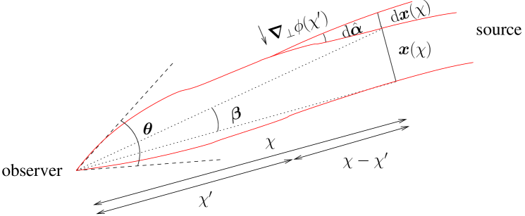
Figure 1: Propagation of two light rays (red solid lines), converging on the observer on the left. The light rays are separated by the transverse comoving distance $\bm{x}$, which varies with distance $\chi$ from the observer. An exemplary deflector at distance $\chi^{\prime}$ perturbes the geodescics proportional to the transverse gradient $\bm{\nabla}_{\perp}\phi$ of the potential. The dashed lines indicate the apparent direction of the light rays, converging on the observer under the angle $\bm{\theta}$. The dotted lines show the unperturbed geodesics, defining the angle $\bm{\beta}$ under which the unperturbed transverse comoving separation $\bm{x}$ is seen.

1.3.3 Linearized lensing quantities

The integral equation (11) can be approximated by substituting the separation vector $\bm{x}$ in the integral by the $0^{\rm th}$-order solution $\bm{x}_{0}(\chi)=f_{K}(\chi)\bm{\theta}$ (10). This corresponds to integrating the potential gradient along the unperturbed ray, which is called the Born approximation (see Sect. 1.3.10 for higher-order corrections). Further, we linearise the lens equation (12) and define the (inverse) amplification matrix as the Jacobian $\bm{\mathrm{A}}=\partial\bm{\beta}/\partial\bm{\theta}$, which describes a linear mapping from lensed (image) coordinates $\bm{\theta}$ to unlensed (source) coordinates $\bm{\beta}$,

$$A_{ij} = \frac{\partial\beta_{i}}{\partial\theta_{j}}=\delta_{ij}-\frac{\partial\alpha_{i}}{\partial\theta_{j}}$$ (14)

$$= \delta_{ij}-\frac{2}{c^{2}}\int_{0}^{\chi}{\rm d}\chi^{\prime}\frac{f_{K}(\chi-\chi^{\prime})f_{K}(\chi^{\prime})}{f_{K}(\chi)}\frac{\partial^{2}}{\partial x_{i}\partial x_{j}}\Phi(f_{K}(\chi^{\prime})\bm{\theta},\chi^{\prime}).$$

The second term in (13) drops out since it does not depend on the angle $\bm{\theta}$.

In this approximations the deflection angle can be written as the gradient of a 2D potential, the lensing potential $\psi$,

$$\psi(\bm{\theta},\chi)=\frac{2}{c^{2}}\int_{0}^{\chi}{\rm d}\chi^{\prime}\frac{f_{K}(\chi-\chi^{\prime})}{f_{K}(\chi)f_{K}(\chi^{\prime})}\,\Phi(f_{K}(\chi^{\prime})\bm{\theta},\chi^{\prime}).$$ (15)

With this definition, the Jacobi matrix can be expressed as

$$A_{ij}=\delta_{ij}-\partial_{i}\partial_{j}\psi,$$ (16)

where the partial derivatives are understood with respect to $\bm{\theta}$. The symmetrical matrix ${\bm{\mathrm{A}}}$ is parametrized in terms of the scalar convergence, $\kappa$, and the two-component spin-two shear, $\gamma=(\gamma_{1},\gamma_{2})$, as

$$\bm{\mathrm{A}}=\left(\begin{array}[]{cc}1-\kappa-\gamma_{1}&-\gamma_{2}\\ -\gamma_{2}&1-\kappa+\gamma_{1}\end{array}\right).$$ (17)

This defines the convergence and shear as second derivatives of the potential,

$$\kappa=\frac{1}{2}\left(\partial_{1}\partial_{1}+\partial_{2}\partial_{2}\right)\psi=\frac{1}{2}\nabla^{2}\psi;\;\;;\gamma_{1}=\frac{1}{2}\left(\partial_{1}\partial_{1}-\partial_{2}\partial_{2}\right)\psi;\;\;\gamma_{2}=\partial_{1}\partial_{2}\psi.$$ (18)

The inverse Jacobian $\bm{\mathrm{A}}^{-1}$ describes the local mapping of the source light distribution to image coordinates. The convergence, being the diagonal part of the matrix, is an isotropic increase or decrease of the observed size of a source image. Shear, the trace-free part, quantifies an anisotropic stretching, turning a circular into an elliptical light distribution.

It is mathematically convenient to write the shear as complex number, $\gamma=\gamma_{1}+\rm i\gamma_{2}=|\gamma|\exp(2\rm i\varphi)$, with $\varphi$ being the polar angle between the two shear components. Shear transforms as a spin-two quantity: a rotation about $\pi$ is the identity transformation of an ellipse (see Fig. 2 for an illustration).

Figure 2: The orientation of the ellipses given by the Cartesian coordinates ${\gamma_{1}}$ and ${\gamma_{2}}$ of the shear. While the polar angle $\varphi$ passes through the range $[0;\,2\pi]$, the shear ellipse rotates around $\pi$.

In the context of cosmological lensing by large-scale structures, images are very weakly lensed, and the values of $\kappa$ and $\gamma$ are on the order of a few percent or less. Each source is mapped uniquely onto one image, there are no multiple images, and the matrix $\bm{\mathrm{A}}$ is indeed invertible.

We can factor out $(1-\kappa)$ from $\bm{\mathrm{A}}$ (17), since this multiplier only affects the size but not the shape of the source. Cosmic shear is based on the measurement of galaxy shapes (see Sect. 4.1), and therefore the observable in question is not the shear $\gamma$ but the reduced shear,

$$g=\frac{\gamma}{1-\kappa},$$ (19)

which has the same spin-two transformation properties as shear. Weak lensing is the regime where the effect of gravitational lensing is very small, with both the convergence and the shear much smaller than unity. Therefore, shear is a good approximation of reduced shear to linear order (see Sect. 1.3.10 for its validity).

1.3.4 Projected overdensity

Since the convergence $\kappa$ is related to the lensing potential $\psi$ (15) via a 2D Poisson equation (18), it can be interpreted as a (projected) surface density. To introduce the 3D density contrast $\delta$, we apply the 2D Laplacian of the lensing potential (15) to the 3D potential $\Phi$ and add the second-order deriviate along the comoving coordinate, $\partial^{2}/\partial\chi^{2}$. This additional term vanishes, since positive and negative contributions cancel out to a good approximation when integrating along the line of sight. Next, we replace the 3D Laplacian of $\Phi$ with the over-density $\delta$ using the Poisson equation (5), and $\bar{\rho}\propto a^{-3}$. Writing the mean matter density in terms of the critical density, we get

$$\kappa(\bm{\theta},\chi)=\frac{3H_{0}^{2}\Omega_{\rm m}}{2c^{2}}\int\limits_{0}^{\chi}\frac{{\rm d}\chi^{\prime}}{a(\chi^{\prime})}\frac{f_{K}(\chi-\chi^{\prime})}{f_{K}(\chi)}f_{K}(\chi^{\prime})\,\delta(f_{K}(\chi^{\prime})\bm{\theta},\chi^{\prime}).$$ (20)

This expression is a projection of the density along comoving coordinates, weighted by geometrical factors involving the distances between source, deflector, and observer. In the case of a flat universe, the geometrical weight $(\chi-\chi^{\prime})\chi^{\prime}$ is a parabola with maximum at $\chi^{\prime}=\chi/2$. Thus, structures at around half the distance to the source are most efficient to generate lensing distortions.

The mean convergence from a population of source galaxies is obtained by weighting the above expression with the galaxy probability distribution in comoving distance, $n(\chi){\rm d}\chi$,

$$\kappa(\bm{\theta})=\int\limits_{0}^{\chi_{\rm lim}}{\rm d}\chi\,n(\chi)\,\kappa(\bm{\theta},\chi).$$ (21)

The integral extends out to the limiting comoving distance $\chi_{\rm lim}$ of the galaxy sample. Inserting (20) into (21) and interchanging the integral order results in the following expression,

$$\kappa(\bm{\theta})=\frac{3H_{0}^{2}\Omega_{\rm m}}{2c^{2}}\int\limits_{0}^{\chi_{\rm lim}}\frac{{\rm d}\chi}{a(\chi)}q(\chi)f_{K}(\chi)\,\delta(f_{K}(\chi)\bm{\theta},\chi).$$ (22)

The lens efficiency $q$ is defined as

$$q(\chi)=\int\limits_{\chi}^{\chi_{\rm lim}}{\rm d}\chi^{\prime}\,n(\chi^{\prime})\frac{f_{K}(\chi^{\prime}-\chi)}{f_{K}(\chi^{\prime})},$$ (23)

and indicates the lensing strength at a distance $\chi$ of the combined background galaxy distribution. Thus, the convergence is a linear measure of the total matter density, projected along the line of sight with dependences on the geometry of the universe via the distance ratios, and the source galaxy distribution $n(\chi){\rm d}\chi=n(z){\rm d}z$. The latter is usually obtained using photometric redshifts (Sect. 4.5.1). We will see in Sect. 1.3.8 how to recover information in the redshift direction.

By construction, the expectation value of shear and convergence are zero, since $\langle\delta\rangle=0$. The first non-trivial statistical measure of the distribution of $\kappa$ and $\gamma$ are second moments. Practical estimators of weak-lensing second-order statistics in real and Fourier-space are discussed in Sects. 1.3.7 and 2.1.

1.3.5 Estimating shear from galaxies

In the case of cosmic shear, not the convergence but the shear is measured from the observed galaxy shapes, as discussed in this section. Theoretical predictions of the convergence (22) can be related to the observed shear using the relations (18). Further, a convergence field can be estimated by reconstruction from the observed galaxy shapes.

We can attribute an intrinsic, complex source ellipticity $\varepsilon^{\rm s}$ to a galaxy. Cosmic shear modifies this ellipticity as a function of the complex reduced shear, which depends on the definition of $\varepsilon^{\rm s}$. If we define this quantity for an image with elliptical isophotes, minor-to-major axis ratio $b/a$, and position angle $\phi$, as $\varepsilon=(a-b)/(a+b)\times\exp(2{\rm i}\phi)$, the observed ellipticity $\varepsilon$ (for $|g|\leq 1)$ is given as [1997A&A...318..687S]

$$\varepsilon=\frac{\varepsilon^{\rm s}+g}{1+g^{\ast}\varepsilon^{\rm s}}.$$ (24)

The asterisk “^∗” denotes complex conjugation. In the weak-lensing regime, this relation is approximated to

$$\varepsilon\approx\varepsilon^{\rm s}+\gamma.$$ (25)

If the intrinsic ellipticity of galaxies has no preferred orientation, the expectation value of $\varepsilon^{\rm s}$ vanishes, $\langle\varepsilon^{\rm s}\rangle=0$, and the observed ellipticity is an unbiased estimator of the reduced shear,

$$\left\langle\varepsilon\right\rangle=g.$$ (26)

This relation breaks down in the presence of intrinsic galaxy alignments (Sect. 1.3.9).

Another commonly used ellipticity estimator has been proposed by [1995A&A...294..411S]. This estimator has a slightly simpler dependence on second moments of galaxy images, which have been widely used for shape estimation, see Sect. 4.1. However, it it does not provide an unbiased estimator of $g$, but explicitly depends on the intrinsic ellipticity distribution.

In the weak-lensing regime, the shear cannot be detected from an individual galaxy. With distortions induced by the LSS of the order $\gamma\sim 0.03$, and the typical intrinsic ellipticity rms of $\sigma_{\varepsilon}=\langle|\varepsilon|^{2}\rangle^{1/2}\sim 0.3$, one needs to average over a number of galaxies $N$ of at least a few hundred to obtain a signal-to-noise ratio $S/N=\gamma\times N^{1/2}/\sigma_{\varepsilon}$ of above unity.

1.3.6 E- and B-modes

The Born approximation introduced in Sect. 1.3.3 results in the definition of the convergence and shear to be functions of a single scalar potential (15). The two shear components defined in that way (18) are not independent, and the shear field cannot have an arbitrary form. We can define a vector field $\bm{u}$ as the gradient of the “potential” $\kappa$, $\bm{u}=\bm{\nabla}\kappa$. By definition, the curl of this gradient vanishes, $\bm{\nabla}\times\bm{u}=\partial_{1}u_{2}-\partial_{2}u_{1}=0$. Inserting the relations between $\kappa,\gamma$ and $\psi$ (18) into this equality results in second-derivative constraints for $\gamma$. A shear field fulfilling those relations is called an E-mode field, analogous to the electric field. In real life however, $\bm{u}$ obtained from observed data is in general not a pure gradient field but has a non-vanishing curl component. The corresponding convergence field can be decomposed into its E-mode component, $\kappa^{\rm E}$, and B-mode, $\kappa^{\rm B}$, given by $\nabla^{2}\kappa^{\rm E}=\bm{\nabla}u$ and $\nabla^{2}\kappa^{\rm B}=\bm{\nabla}\times u$.. The B-mode component can have various origins:

1. Higher-order terms in the light-propagation equation (11), e.g. lens-lens coupling and integration along the perturbed light path (17) [2010A&A...523A..28K].

2. Other higher-order terms beyond usual approximations of relations such as between shear and reduced shear, or between shear and certain ellipticity estimators (see Sect. 4.1) [2010A&A...523A..28K].

3. Lens galaxy selection biases, such as size and magnitude bias [2003ApJ...583...58W, 2009ApJ...702..593S], or clustering of lensing galaxies [1998A&A...338..375B, 2002A&A...389..729S].

4. Correlations of the intrinsic shapes of galaxies with each other, and with the structures that induce weak-lensing distortions (intrinsic alignment, Sect. 1.3.9) [2002ApJ...568...20C].

5. Image and data analysis errors such as PSF correction residuals, systematics in the astrometry.

The astrophysical effects (i) - (iv) cause a B-mode at the percent-level compared to the E-mode. The intrinsic alignment B-mode amplitude is the least well-known since the model uncertainty is large [2013MNRAS.435..194C]. Up to now, cosmic shear surveys do not have the statistical power to reliably detect those B-modes. Until recently, the amplitude of a B-mode detection has exclusively been used to assess the quality of the data analysis, assuming that (v) is the only measurable B-mode contributor. While this is a valid approach, it only captures those systematics that create a B-mode. A B-mode non-detection might render an observer over-confident to believe that also the E-mode is uncontaminated by systematics. Further, the ratio of B- to E-mode should not be used to judge the data quality, since this ratio is not cosmology-independent and can bias the cosmological inference of the data.

Some of my past work focused on studying and developing estimators that separate E- from B-mode in shear data. This will be presented in Sect. 2.2.

1.3.7 The lensing power spectrum

The basic second-order function of the convergence (22) is the two-point correlation function (2PCF) $\langle\kappa(\bm{\vartheta})\kappa(\bm{\vartheta}+\bm{\theta})\rangle$. The brackets denote ensemble average, which can be replaced by a spatial average over angular positions $\bm{\vartheta}$. With the assumption that the density field $\delta$ on large scales is statistically homogeneous and isotropic, which follows from the cosmological principle, the same holds for the convergence. The 2PCF is then invariant under translation and rotation, and therefore a function of only the modulus of the separation vector between the two lines of sight $\theta$. Expressed in Fourier space, the two-point correlation function defines the flat-sky convergence power spectrum $P_{\kappa}$ with

$$\left\langle\tilde{\kappa}(\bm{\ell})\tilde{\kappa}^{\ast}(\bm{\ell}^{\prime})\right\rangle=(2\pi)^{2}\delta_{\rm D}(\bm{\ell}-\bm{\ell}^{\prime})P_{\kappa}(\ell).$$ (27)

Here, $\delta_{\rm D}$ is the Dirac delta function. The complex Fourier transform $\tilde{\kappa}$ of the convergence is a function of the 2D wave vector $\bm{\ell}$, the Fourier-conjugate of $\bm{\theta}$. Again due to statistical homogeneity and isotropy, the power spectrum only depends on the modulus $\ell$. For simplicity, we ignore the curvature of the sky in this expression. For lensing on very large scales, and for 3D lensing (Sect. 1.3.8), the curvature has to be accounted for by more accurate expressions [2008PhRvD..78l3506L], or by applying spherical harmonics instead of Fourier transforms.

If the convergence field is decomposed into an E-mode $\kappa^{\rm E}$ and B-mode component $\kappa^{\rm B}$, two expressions analogous to (27) define the E- and B-mode power spectra, $P_{\kappa}^{\rm E}$ and $P_{\kappa}^{\rm B}$.

Taking the square of (22) in Fourier space, we get the power spectrum of the density contrast, $P_{\delta}$, on the right-hand side of the equation. Inserting the result into (27) we obtain the flat-sky convergence power spectrum in terms of the density power spectrum as

$$P_{\kappa}(\ell)=\frac{9}{4}\,\Omega_{\rm m}^{2}\left(\frac{H_{0}}{c}\right)^{4}\int_{0}^{\chi_{\rm lim}}{\rm d}\chi\,\frac{q^{2}(\chi)}{a^{2}(\chi)}P_{\delta}\left(k=\frac{\ell}{f_{K}(\chi)},\chi\right).$$ (28)

This simple result can be derived using a few approximations: the Limber projection is applied, which only collects modes that lie in the plane of the sky, thereby neglecting correlations along the line of sight [1953ApJ...117..134L, 1992ApJ...388..272K, 2007A&A...473..711S, 2012MNRAS.422.2854G]. In addition, the small-angle approximation (expanding to first order trigonometric functions of the angle) and the flat-sky limit (replacing spherical harmonics by Fourier transforms) are used. A further assumption is the absence of galaxy clustering, therefore ignoring source-source [2002A&A...389..729S], and source-lens [1998A&A...338..375B, H02] clustering. Theoretical predictions for the power spectrum are shown in Fig. 3, using linear theory, and the non-linear fitting formulae of 2012ApJ…761..152T. See Sect. 1.3.8 for the definition of the tomographic redshift bins.

The projection (28) mixes different 3D $k$-modes into 2D $\ell$ wavemodes along the line-of-sight integration, thereby washing out many features present in the 3D density power spectrum. For example, baryonic acoustic oscillations are smeared out and are not seen in the lensing spectrum [2006ApJ...647L..91S, 2009NewA...14..507Z]. This reduces the sensitivity of $P_{\kappa}$ with respect to cosmological parameters, for example compared to the CMB anisotropy power spectrum. Examples for some parameters are shown in Fig. 3. Then two main response modes of $P_{\kappa}$ for changing parameters are an amplitude change, caused by $\sigma_{8}$, $\Omega_{\rm m}$, and $w_{0}$, and a tilt, generated by $n_{\rm s}$, and $h$ (and, consequently, shifts are seen when varying the physical density parameters $\omega_{\rm m}$ and $\omega_{\rm b}$). The parameter combination that $P_{\kappa}$ is most sensitive to is $\sigma_{8}\Omega_{\rm m}^{\alpha}$, with $\alpha\approx 0.75$ in the linear regime [1997A&A...322....1B].

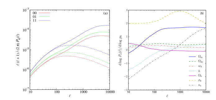
Figure 3: (a) The scaled tomographic convergence auto- and cross-power spectrum $\ell(\ell+1)/(2\pi)P_{\kappa,ij}(\ell)$ for two redshift bins $(i,j)=(0,1)$ with redshift ranges $z_{0}=[0.5;0.7]$, and $z_{1}=[0.9;1.1]$ for a Euclid-like source redshift distribution. Solid (dashed) lines correspond to the non-linear (linear) model. (b) Derivatives ${\rm d}\log P_{\kappa}/{\rm d}\log p_{k}$ of the convergence power spectrum with respect to various cosmological parameters $p_{k}$, as indicated in the figure. The corresponding redshift bin is $[0.9;1.1]$.

Writing the relations between $\kappa$, $\gamma$ and the lensing potential $\psi$ (18) in Fourier space, and using complex notation for the shear, one finds for $\ell\neq 0$

$$\tilde{\gamma}(\bm{\ell})=\frac{\left(\ell_{1}+{\rm i}\,\ell_{2}\right)^{2}}{\ell^{2}}\tilde{\kappa}(\bm{\ell})={\rm e}^{2{\rm i}\beta}\tilde{\kappa}(\bm{\ell}),$$ (29)

with $\beta$ being the polar angle of the wave-vector $\bm{\ell}=(\ell_{1},\ell_{2})$, written as complex quantity. Therefore, we get the very useful fact that the power spectrum of the shear equals the one of the convergence, $P_{\gamma}=P_{\kappa}$.

The shear power spectrum can in principle be obtained directly from observed ellipticities 2001ApJ…554…67He.g., or via pixellised convergence maps in Fourier space that have been reconstructed from the observed ellipticities, e.g. 1998ApJ…506…64S. However, the simplest and most robust way to estimate second-order shear correlations are in real space, which we will discuss in the following section.

1.3.8 Shear tomography

The redshift distribution of source galaxies determines the redshift range over which the density contrast is projected onto the 2D convergence and shear. By separating source galaxies according to their redshift, we obtain lensing fields with different redshift weighting via the lens efficiency (23), thus probing different epochs in the history of the Universe with different weights. Despite the two-dimensional aspect of gravitational lensing, this allows us to recover a 3D tomographic view of the large-scale structure In particular, it helps us to measure subtle effects that are projected out in 2D lensing, such as the growth of structures, or a time-varying dark-energy state parameter $w(z)$.

If we denote the redshift distribution in each of $N_{z}$ bin with $p_{i},i=1\ldots N_{z}$, we obtain a new lensing efficiency $q_{i}$ (23) for each case, and a resulting projected overdensity $\kappa_{i}$. This leads to $N_{z}(N_{z}-1)/2$ convergence power spectra $P_{\kappa,ij},1\leq i\leq j\leq N_{z}$, including not only the auto-spectra ($i=j$) but also the cross-spectra ($i\neq j$). In (28), $q^{2}$ is replaced by the product $q_{i}q_{j}$ [1998ApJ...506...64S, 1999ApJ...522L..21H].

1.3.9 Intrinsic alignment

Shapes of galaxies can be correlated in the absence of gravitational lensing, due to gravitational interactions between galaxies and the surrounding tidal fields. The intrinsic alignment (IA) of galaxy shapes adds an excess correlation to the cosmic shear signal that, if not taken into account properly, can bias cosmological inferences by tens of per cent. IA is difficult to account for, since it cannot simply be removed by a sophisticated galaxy selection, nor can it be easily predicted theoretically since it depends on details of galaxy formation.

Due to IA, the intrinsic ellipticity of galaxies $\varepsilon^{\rm s}$ no longer has a random orientation, or phase. This directly contributes to the measured two-point shear correlation function (34), as follows. The first term in (35) describes the correlation of intrinsic ellipticities of two galaxies $i$ and $j$. This term ($II$, or shape-shape correlation) is non-zero only for physically close galaxies. Its contribution to cosmic shear ($GG$, or shear-shear correlation), the last term in (35), can be suppressed by down-weighting or omitting entirely galaxy pairs at the same redshift [HH03, KS02, KS03].

The second and third term in (35) correspond to the correlation between the intrinsic ellipcitiy of one galaxy with the shear of another galaxy. For either of these terms ($GI$, or shape-shear correlation) to be non-zero, the foreground galaxy ellipticity has to be correlated via IA to structures that shear a background galaxy. A lensing mass distribution causes background galaxies to be aligned tangentially. Foreground galaxies at the same redshift as the mass distribution are strechted radially towards the mass by tidal forces. Therefore the ellipticities of background and foreground galaxies tend to be orthogonal, corresponding to a negative $GI$ correlation. For typical cosmic shear surveys with not too small redshift bins, $GI$ dominates over $II$. Overall, the intrinsic alignment of galaxy orientations contribute to the lensing power spectrum typically to up to 10%.

1.3.10 Higher-order corrections

The approximations made in Sects. 1.3.3 and 1.3.7, resulting in the convergence power spectrum, have to be tested for their validity. Corrections to the linearised propagation equation (17) include couplings between lens structures at different redshift (lens-lens coupling), and integration along the perturbed ray (additional terms to the Born approximation). Further, higher-order correlations of the convergence take account of the reduced shear as observable. Similar terms arise from the fact that the observed size and magnitudes of lensing galaxies are correlated with the foreground convergence field 2001MNRAS.326..326H,2009PhRvL.103e1301Smagnification and size bias; . Over the relevant scale range ($\ell\leq 10^{4}$) most of those effects are at least two orders of magnitude smaller than the first-order E-mode convergence power spectrum, and create a B-mode spectrum of similar low amplitude. The largest contribution is the reduced-shear correction, which attains nearly $10\%$ of the shear power spectrum on arc minute scales [1997A&A...322....1B, 1998MNRAS.296..873S, 2006PhRvD..73b3009D, 2010A&A...523A..28K]. In K10 I present simple fitting formulae that provide the reduced-shear power spectrum to $2\%$ accuracy for $\ell<2\times 10^{5}$ for $\Lambda$CDM cosmological parameters within the WMAP7 68% error ellipsoid.

Thanks to the broad lensing kernel, the Limber approximation is very precise and deviates from the full integration only on very large scales, for $\ell<20$ [2012MNRAS.422.2854G, 2012PhRvD..86b3001B]. Similary, the flat-sky approximation for the lensing power spectrum (28) and correlation function (36) provides sub-percent level accuracy on all but the very largest scales [KH17, 2016arXiv161104954K, 2017JCAP...05..014L]. The full GR treatment of fluctuations together with dropping the small-angle approximation was also found to make a difference only on very large scales [2010PhRvD..81h3002B]. In KH17 I showed that using the Limber and flat-sky approximations, current cosmological results are unaffected. I developed the second-order Limber approximation for cosmic shear, and demonstrated that this will also sufficient for future surveys, since the corresponding errors are sub-dominant compared to cosmic variance on all scales, see Fig. 4.

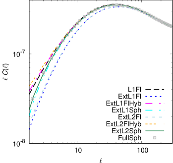
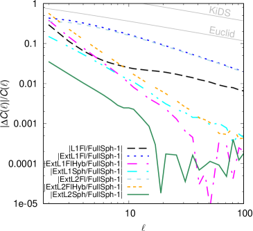
Figure 4: The shear power spectrum for different approximations. Limber to first order: standard with flat-sky (L1Fl), extended for flat sky (ExtL1Fl), extended hybrid for flat sky (ExtL1FlHyb), and extended in the spherical expansion (ExtL1Sph); second-order Limber approximations: extended flat sky (ExtL2Fl), extended hybrid flat sky (ExtL2FlHyb), and extended spherical expansion (ExtL2Sph); full (exact) spherical projection (FullSph). The left panel shows the total shear power spectrum. The right panel shows the fractional difference resulting from each approximation, relative to the full spherical projection of the shear power spectrum. The two light grey curves on the top show the cosmic variance for KiDS- and Euclid-like surveys with areas of $1,500$ and $15,000$ square degrees, respectively. From [KH17].

Many of the above mentioned corrections are more important for third-order lensing statistics [H02, 2005PhRvD..72h3001D, 2013arXiv1306.6151V], which are presented in Sect. 2.3.1. In CFHTLenS-2+3pt we accounted for source-lens clustering terms contributing to the lensing bispectrum. Ignoring this contamination, the parameter $\Sigma_{8}$ (see eq. (75)) was biased high by 0.03, which is subdominant compared to the statistical errors.

2 Shear correlation estimators

2.1 The shear correlation function

The most basic, non-trivial cosmic shear observable is the real-space shear two-point correlation function (2PCF), since it can be estimated by simply multiplying the ellipticities of galaxy pairs and averaging.

The two shear components of each galaxy are conveniently decomposed into tangential component, $\gamma_{\rm t}$, and cross-component, $\gamma_{\times}$. With respect to a given direction vector $\bm{\theta}$ whose polar angle is $\phi$, they are defined as

$$\gamma_{\rm t}=-\Re\left(\gamma\,{\rm e}^{-2{\rm i}\phi}\right);\quad\gamma_{\times}=-\Im\left(\gamma\,{\rm e}^{-2{\rm i}\phi}\right).$$ (30)

The minus sign, by convention, results in a positive value of $\gamma_{\rm t}$ for the tangential alignment around a mass overdensity. Radial alignment around underdensities have a negative $\gamma_{\rm t}$. A positive cross-component shear is rotated by $+\pi/4$ with respect to the tangential component.

Three two-point correlators can be formed from the two shear components, $\langle\gamma_{\rm t}\gamma_{\rm t}\rangle$, $\langle\gamma_{\times}\gamma_{\times}\rangle$ and $\langle\gamma_{\rm t}\gamma_{\times}\rangle$. The latter vanishes in a parity-symmetric universe, where the shear field is statistically invariant under a mirror transformation. Such a transformation leaves $\gamma_{\rm t}$ invariant but changes the sign of $\gamma_{\times}$. The two non-zero two-point correlators are combined into the two components of the shear 2PCF [1991ApJ...380....1M],

$$\eqalign{\xi}_{+}(\theta) =\langle\gamma\gamma^{\ast}\rangle(\theta) =\langle\gamma_{\rm t}\gamma_{\rm t}\rangle(\theta)+\langle\gamma_{\times}\gamma_{\times}\rangle(\theta);\quad$$ (32)

$$\xi_{-}(\theta) =\Re\left[\langle\gamma\gamma\rangle(\theta){\rm e}^{-4{\rm i}\phi}\right] =\langle\gamma_{\rm t}\gamma_{\rm t}\rangle(\theta)-\langle\gamma_{\times}\gamma_{\times}\rangle(\theta).$$ (33)

The two components are plotted in Fig. 5. We note here that from the equality of the shear and convergence power spectrum and Parseval’s theorem, it follows that $\xi_{+}$ is identical to the two-point correlation function of $\kappa$.

We defined an estimator of the 2PCF in SvWKM02 as

$$\hat{\xi}_{\pm}(\theta)=\frac{\sum_{ij}w_{i}w_{j}\left(\varepsilon_{{\rm t},i}\varepsilon_{{\rm t},j}\pm\varepsilon_{\times,i}\varepsilon_{\times,j}\right)}{\sum_{ij}w_{i}w_{j}}.$$ (34)

The sum extends over pairs of galaxies ($i,j$) at positions on the sky $\bm{\vartheta}_{i}$ and $\bm{\vartheta}_{j}$, respectively, whose separation $|\bm{\vartheta}_{i}-\bm{\vartheta}_{j}|$ lies in an angular distance bin around $\theta$. Each galaxy has a measured ellipticity $\varepsilon_{i}$, and an attributed weight $w_{i}$, which may reflect the measurement uncertainty. Using the weak-lensing relation (25) and taking the expectation value of (34), we get terms of the following type, exemplarily stated for $\xi_{+}$:

$$\langle\varepsilon^{(\rm s)}_{i}{\varepsilon_{j}^{(\rm s)}}^{\ast}\rangle;\langle\varepsilon^{(\rm s)}_{i}\gamma_{j}^{\ast}\rangle;\langle\gamma_{i}{\varepsilon_{j}^{(\rm s)}}^{\ast}\rangle;\quad\mbox{and}\quad\langle\gamma_{i}\gamma_{j}^{\ast}\rangle.$$ (35)

We discuss the first three terms in Sect. 1.3.9, in the context of intrinsic alignment (IA). In the absence of IA, those three terms vanish and the last term is equal to $\xi_{+}(|\bm{\vartheta}_{i}-\bm{\vartheta}_{j}|))$. The analogous case holds for $\xi_{-}$.

The main advantage of the simple estimator (34) is that it does not require the knowledge of the mask geometry, but only whether a given galaxy is within the masked area or not. For that reason, many other second-order estimators that we discuss in the following are based in this one.

The survey and mask geometry is however important to compute the covariance of (34). This influence was studied in detail in KS04, where I developed a Monte-Carlo method to compute the covariance given a galaxy catalogue. This method was subsequently used for a Principal Component Analysis [MK05], and Karhunen-Loève [KM05] study, to examine the dependency of various survey properties on the weak-lensing information content. The same Monte-Carlo method was also used in CFHTLenS to compute the covariance matrix of the 2PCF [CFHTLenS-2pt-notomo].

Using (27) and (29), we write the 2PCF in the flat-sky approximation as Hankel transforms of the convergence power spectrum,

$$\xi_{+}(\theta) =\frac{1}{2\pi}\int{\rm d}\ell\,\ell{\rm J}_{0}(\ell\theta)[P_{\kappa}^{\rm E}(\ell)+P_{\kappa}^{\rm B}(\ell)];\quad$$

$$\xi_{-}(\theta) =\frac{1}{2\pi}\int{\rm d}\ell\,\ell{\rm J}_{4}(\ell\theta)[P_{\kappa}^{\rm E}(\ell)-P_{\kappa}^{\rm B}(\ell)].$$ (36)

These expressions can be easily and quickly integrated numerically using fast Hankel transforms [2000MNRAS.312..257H].

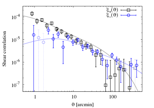
Figure 5: 2PCF components $\xi_{+}$ and $\xi_{-}$ (33) measured in CFHTLenS. The dotted lines show the WMAP7 model prediction [2010arXiv1001.4538K]. From CFHTLenS-2pt-notomo.

The two 2PCF components mix E- and B-mode power spectra in two different ways. To separate the two modes, a further filtering of the 2PCF is necessary, which will be discussed in the following section.

2.2 Derived second-order functions

Apart from the 2PCF (33), other, derived second-order functions have been widely used to measure lensing correlations in past and present cosmic shear surveys. The motivation for derived statistics are to construct observables that (1) have high signal-to-noise for a given angular scale, (2) show small correlations between different scales, and (3) separate into E- and B-modes. In particular the latter property is of interest, since the B-mode can be used to assess the level of (certain) systematics in the data as we have seen in Sect. 1.3.6.

All second-order functions can be written as filtered integrals over the convergence power spectrum, and the corresponding filter functions define their properties.

2.2.1 Aperture-mass dispersion

Another popular statistic is the aperture-mass dispersion, denoted as $\left\langle M_{\rm ap}^{2}\right\rangle(\theta)$ (Fig. 6). First, one defines the aperture mass as mean tangential shear with respect to the centre $\bm{\vartheta}$ of a circular region, weighted by a filter function $Q_{\theta}$ with characteristic scale $\theta$,

$$M_{\rm ap}(\theta,\bm{\vartheta})=\int{\rm d}^{2}\vartheta^{\prime}\,Q_{\theta}(|\bm{\vartheta}-\bm{\vartheta}^{\prime}|)\,\gamma_{\rm t}(\bm{\vartheta}^{\prime})=\int{\rm d}^{2}\vartheta^{\prime}\,U_{\theta}(|\bm{\vartheta}-\bm{\vartheta}^{\prime}|)\,\kappa(\bm{\vartheta}^{\prime}).$$ (37)

The second equality can be derived from the relations between shear and convergence, which defines the filter function $U_{\theta}$ in terms of $Q_{\theta}$ [KSFW94, S96]. The aperture mass is therefore closely related to the local projected over-density, and owes its name to this fact. The function $U_{\theta}$ is compensated (i.e. the integral over its support vanishes, $\int{\rm d}^{2}\vartheta\,U_{\theta}(\bm{\vartheta})=0$), and filters out a constant mass sheet $\kappa_{0}=\mbox{const}$, since the monopole mode ($\ell=0$) is not recoverable from the shear (29). Two choices for the functions $U_{\theta}$, and consequently $Q_{\theta}$, have been widely used for cosmic shear, a fourth-order polynomial [1998MNRAS.296..873S], and a Gaussian function [2002ApJ...568...20C].

By projecting out the tangential component of the shear, $M_{\rm ap}$ is sensitive to the E-mode only. One defines $M_{\times}$ by replacing $\gamma_{\rm t}$ with $\gamma_{\times}$ in (37) as a probe of the B-mode only. The variance of (37) between different aperture centres defines the dispersion $\left\langle M_{\rm ap}^{2}\right\rangle(\theta)$, which can be interpreted as fluctuations of lensing strength between lines of sight, and therefore have an intuitive connection to fluctuations in the projected density contrast.

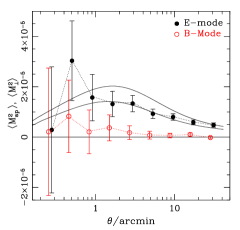
Figure 6: Aperture-mass dispersion that we measured in COSMOS. The two solid lines correspond to predictions with $\sigma_{8}=0.7$ and $0.8$, respectively. From SHJKS09.

A new $\cal N$ estimator that includes both the aperture-mass dispersion at various angular scales, and a measure of the 2PCF at one angular scale $\theta_{0}$, is discussed in EKS08. This new data vector is $\bm{\mathcal{N}}=\left(\langle M_{\rm ap}^{2}\rangle(\theta_{1}),\ldots,\langle M_{\rm ap}^{2}\rangle(\theta_{n}),\xi_{+}(\theta_{0})\right)$. It is a compromise between insensitivity to the B-mode (via the aperture-mass dispersion), and capturing the long-wavelength modes and thus maximizing the information content (through $\xi_{+}$). The tightest constraints on cosmological parameters are obtained with $\theta_{0}$ of around $10$ arcmin.

2.2.2 Practical estimators

The aperture-mass dispersion can in principle be estimated by averaging over many aperture centres $\bm{\vartheta}$. This is however not practical: The sky coverage of a galaxy survey is not contiguous, but has gaps and holes due to masking. Apertures with overlap with masked areas biases the result, and avoiding overlap results in a substantial area loss. This is particularly problematic for filter functions whose support extend beyond the scale $\theta$. One possibility is to fill in the missing data, e.g. with inpainting techniques [2009MNRAS.395.1265P], resulting in a pixelised, contiguous convergence map on which the convolution (37) can be calculated very efficiently [2012MNRAS.423.3405L]. Alternatively, the dispersion measures can be expressed in terms of the 2PCF, and are therefore based on the estimator (34) for which the mask geometry does not play a role.

2.2.3 Generalisations

In fact, every second-order statistic can be expressed as integrals over the 2PCF because, as mentioned above, all are functions of $P_{\kappa}$, and the relation (36) can be inverted. In general, they do not contain the full information about the convergence power spectrum [EKS08], but separate E- and B-modes.

The general expression for an E-/B-mode separating function $X_{\rm E,B}$ is

$$X_{\rm E,B}=\frac{1}{2\pi}\int_{0}^{\infty}{\rm d}\ell\,\ell\,P_{\kappa}^{\rm E,B}(\ell)\tilde{U}^{2}(\ell).$$ (38)

A practical estimator using (34) is

$$\hat{X}_{\rm E,B}=\frac{1}{2}\sum_{i}\vartheta_{i}\,\Delta\vartheta_{i}\left[T_{+}\left({\vartheta_{i}}\right)\hat{\xi}_{+}(\vartheta_{i})\pm T_{-}\left({\vartheta_{i}}\right)\hat{\xi}_{-}(\vartheta_{i})\right].$$ (39)

Here, $\Delta\vartheta_{i}$ is the bin width, which can vary with $i$, for example in the case of logarithmic bins. The filter functions $T_{\pm}$ and $\tilde{U}^{2}$ are Hankel-transform pairs, given by the integral relation [2002ApJ...568...20C, 2002A&A...389..729S]

$$T_{\pm}(x)=\int_{0}^{\infty}{\rm d}t\,t\,{\rm J}_{0,4}(xt)\tilde{U}^{2}(t).$$ (40)

This implicit relation between $T_{+}$ and $T_{-}$ guarantees the separation into E- and B-modes of the estimator (39).

In some cases of $X_{\rm E,B}$, for example for the aperture mass dispersion, the power-spectrum filter $\tilde{U}$ is explicitely given as the Fourier transform of a real-space filter function $U$, see e.g. (37) for the aperture mass. In other cases the functions $T_{\pm}$ are constructed first, and $\tilde{U}$ is calculated by inverting the relation (40). Model predictions of $X_{\rm E}$ can be obtained from either (38), or (39). For the latter, one inserts a theoretical model for $\xi_{\pm}$, and does not need to calculate $\tilde{U}$.

2.2.4 E-/B-mode mixing

None of the derived second-order functions introduced so far provide a pure E-/B-mode separation. They suffer from a leakage between the modes, on small scales, or large scales, or both. This mode mixing comes from the incomplete information on the measured shear correlation: On very small scales, up to 10 arc seconds or so, galaxy images are blended, preventing accurate shape measurements, and thus the shape correlation on those small scales is not sampled. Large scales, at the order of degrees, are obviously only sampled up to the survey size. This leakage can be mitigated by (i) extrapolating the shear correlation to unobserved scales using a theoretical prediction (thereby potentially biasing the result), or (ii) cutting off small and/or large scales of the derived functions (thereby loosing information). Figure 7 shows the example of the aperture-mass dispersion with a polynomial filter, see KSE06.

Figure 7: Top panel: The E-mode aperture-mass dispersion $\langle M_{\rm ap}^{2}(\theta)\rangle$ and the leakage from the E-mode $\langle M_{\rm ap}^{2}(\theta,\theta_{\rm min})\rangle$ to the B-mode $\langle M_{\perp}^{2}(\theta,\theta_{\rm min})\rangle$ due to the small-scale cutoff $\theta_{\rm min}$ of the shear correlation function. Bottom panel: The ratio $\langle M_{\rm ap}^{2}(\theta,\theta_{\rm min})\rangle/\langle M_{\rm ap}^{2}(\theta)\rangle$. From KSE06.

2.2.5 E-/B-mode functions from a finite interval

E-/B-mode mixing can be avoided altogether by defining derived second-order statistics via suitable filter functions $T_{\pm}$ (or, equivalently $U$). For a pure E-/B-mode separation, those filter functions need to vanish on scales where the shear correlation is missing.

The first such set of filter functions was derived geometrically, by defining the E- and B-mode of the shear field on a circle:

$${\cal C}(\theta)={\cal C}_{\rm t}(\theta)+{\cal C}_{\times}(\theta)=\frac{1}{2\pi}\int\limits_{0}^{2\pi}{\rm d}\phi\left(\gamma_{\rm t}+\gamma_{\times}\right)(\theta,\phi),$$ (41)

where the tangential and cross-components of the shear are measured with respect to the center of a circle with radius $\theta$. By construction, ${\cal C}_{\rm t}$ (${\cal C}_{\times}$) projects out the E-mode (B-mode).

If we now correlate the field $C$ for two concentric circles with different radii $\theta_{1}<\theta_{2}$, the resulting second-order E-mode (B-mode) correlations $\langle{\cal C}_{\rm t}(\theta_{1}){\cal C}_{\rm t}(\theta_{2})\rangle$ ($\langle{\cal C}_{\times}(\theta_{1}){\cal C}_{\times}(\theta_{2})$) correlate the shear at two angular positions with minimum separation $\theta_{2}-\theta_{1}$ and maximum distance $\theta_{1}+\theta_{2}$. This circle statistics thus achieves E-/B-mode separation from shear correlations on a finite interval.

In practise, the shear cannot be measured on a infinitely thin line, and the circle is extended to an annulus or ring ${\cal R}$ with finite width. Two disjoint annuli are correlated to form the ring statistics [SK07].

As all second-order functions, the ring statistics can be written in the forms (38) and (39). Corresponding filter functions $U$ and $T_{\pm}$ have been derived in [SK07], the latter of which have finite support.

The exact form of $T_{\pm}$ is given by the geometrical set-up of the two rings. This can be generalized, and $T_{\pm}$ be derived detached from geometry. From the relations between $T_{+}$ and $T_{-}$ and the requirement that both vanish outside a finite interval $[\vartheta_{\rm min};\vartheta_{\rm max}]$, two integral conditions are sufficient to fulfill these conditions [SK07]:

$$\int_{\vartheta_{\rm min}}^{\vartheta_{\rm max}}{\rm d}\vartheta\,\vartheta\,T_{+}(\vartheta)=0=\int_{\vartheta_{\rm min}}^{\vartheta_{\rm max}}{\rm d}\vartheta\,\vartheta^{3}\,T_{+}(\vartheta).$$ (42)

The corresponding relations for $T_{-}$ are

$$\int_{\vartheta_{\rm min}}^{\vartheta_{\rm max}}{{\rm d}\vartheta\over\vartheta}\,T_{-}(\vartheta)=0=\int_{\vartheta_{\rm min}}^{\vartheta_{\rm max}}{{\rm d}\vartheta\over\vartheta^{3}}\,T_{-}(\vartheta).$$ (43)

The first generalised ring statistics was introduced in 2010A&A…510A…7E, who chose the lowest-order polynomials for $T_{+}$ to fulfill (42) (which is second order).

An optimization scheme for a general ring statistics was developed in FK10. In this work we wrote $T_{+}$ as linear combination of orthogonal polynomials, in this case, Chebyshev polynomials of the second kind, up to order $N-1$. The two integral conditions on $T_{\pm}$ then become a ($N\times 2$) matrix equations in the expansion coefficients. It was determined that $N=6$ captures most of the information of the shear correlation.

Optimisation is then performed by varying the coefficients to maximize two quantities for a given maximum angular scale $\Psi_{\rm max}$, the $S/N$ of the ring statistic and the Fisher matrix figure of merit (FoM) for $\Omega_{\rm m}$ and $\sigma_{8}$. For the Fisher matrix, the (Gaussian) covariance between different scales was accounted for. Fig. 8 shows the FoM as function of $\Psi_{\rm max}$ for different statistics. As expected, the FoM increases with $\Psi_{\rm max}$ as more and more information is included, but the increase flattens out after around 20 arcmin. Compared to the original ring statistic from SK07 (denoted by $Z_{+}$), the optimised ring statistic (denoted by $T_{+}$) achieves two to three times larger FoMs. Depending on the range of scales $\eta=\vartheta_{\rm min}/\vartheta_{\rm max}$, it even outperformed the aperture-mass dispersion.

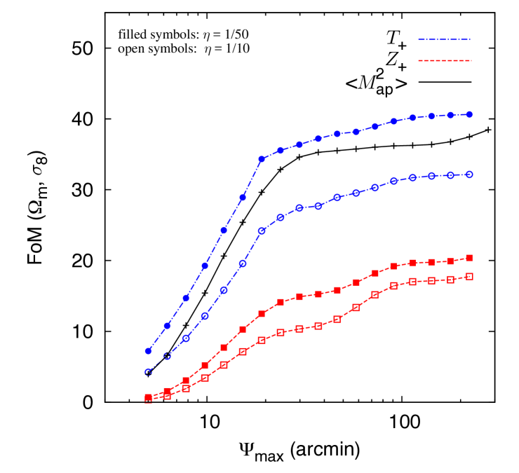
Figure 8: Figure of merit (FoM) for the optimised filter function $T_{+}$ (blue curves), and the original ring statistic filter function $Z_{+}$ from SK07 (in red), as function of the maximum angular scale $\Psi_{\rm max}$. Filled and open symbols represent $\eta\equiv\vartheta_{\rm min}/\vartheta_{\rm max}=1/50$ and $1/10$, respectively. The black curve with crosses corresponds to the aperture-mass with aperture diameter $\vartheta_{\rm max}$. From FK10.

A more general question to ask is, given an interval $[\vartheta_{\rm min};\vartheta_{\rm max}$], how can we capture all available information of the E-mode shear correlation on that interval? The information on a subset of scales, say with $\Psi<\theta_{\rm max}$ should be contained in the entire interval, since all information on $[\vartheta_{\rm min};\vartheta_{\rm max}$ contains a signal with a filter function that is zero for $\theta>\Psi$.

Such general E-/B-mode separating second-order quantities from a finite interval are the so-called COSEBIs COSEBIsComplete Orthogonal Sets of E-/B-mode integrals;. Fig. 9 shows the COSEBIs measured with CFHTLenS. COSEBIs do not depend on a continuous angular scale parameter $\theta$, but are a discrete set of modes $E_{n},B_{n},n=1,2\ldots$ Typically, fewer than 10 COSEBI modes are sufficient to capture all second-order E-mode information [2012A&A...542A.122A].

The COSEBI modes are strongly correlated, which makes visual inspection of the data and comparison to the prediction difficult. Therefore, I compute uncorrelated data points $E^{\rm ortho}_{m}$ as orthogonal transformation of the COSEBIs $E_{n}$, $E^{\rm ortho}_{m}=S_{mn}E_{n}$, where ${\bm{\mathrm{S}}}$ is an orthogonal matrix, ${\bm{\mathrm{S}}}{\bm{\mathrm{S}}}^{\rm T}=1$. The result is presented in the right panel of Fig. 9. Increasing modes $m$ have larger error bars, which correspond to the elements of the diagonal matrix ${\Sigma}$, obtained by diagonalising the COSEBIs covariance matrix ${\bm{\mathrm{C}}}={\bm{\mathrm{S}}}{\Sigma}{\bm{\mathrm{S}}}^{\rm T}$.

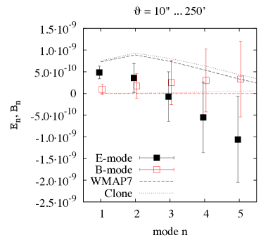
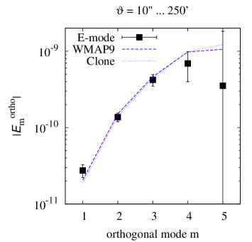
Figure 9: The first five COSEBIs modes, measured in CFHTLenS, together with predictions using a WMAP7 and WMAP9 cosmology, and the CFHTLenS “Clone” $N$-body simulation. Left panel: The original COSEBI modes, from CFHTLenS-2pt-notomo. Right panel: The corresponding tranformed, orthogonal COSEBI modes, from CFHTLenS-2+3pt.

2.3 Higher-order correlations

2.3.1 Third-order correlations

The convergence power spectrum $P_{\kappa}$ (28) only captures the Gaussian component of the LSS. There is however substantial complementary non-Gaussian information in the matter distribution, in particular on small scales, where the non-linear evolution of structures creates non-Gaussian weak-lensing correlations. On small and intermediate scales, these non-linear structures are the dominant contributor to non-Gaussian lensing signatures, compared to (quasi)-linear perturbations, or potential primordial non-Gaussianity. Constraints on the latter from cosmic shear alone can not compete with constraints from other probes such as CMB or galaxy clustering [2004MNRAS.348..897T, 2011MNRAS.411..595P, 2012MNRAS.426.2870H].

To measure these non-Gaussian characteristics, one has to go beyond the second-order convergence power spectrum. The next-leading order statistic is the bispectrum $B_{\kappa}$, which is defined by the following equation:

$$\left\langle\tilde{\kappa}(\bm{\ell}_{1})\tilde{\kappa}(\bm{\ell}_{3})\tilde{\kappa}(\bm{\ell}_{3})\right\rangle=(2\pi)^{2}\delta_{\rm D}(\bm{\ell}_{1}+\bm{\ell}_{2}+\bm{\ell}_{3})\left[B_{\kappa}(\bm{\ell}_{1},\bm{\ell}_{2})+B_{\kappa}(\bm{\ell}_{2},\bm{\ell}_{3})+B_{\kappa}(\bm{\ell}_{3},\bm{\ell}_{1})\right].$$ (44)

The bispectrum measures three-point correlations of the convergence defined on a closed triangle in Fourier space. $B_{\kappa}$ can be related to the density bispectrum $B_{\delta}$ via Limber’s equation [2001ApJ...548....7C]. Other measures of non-Gaussianity are presented in Sect. 2.3.3.

The corresponding real-space weak-lensing observable is the shear three-point correlation function (3PCF) [2003MNRAS.340..580T, tpcf1, 2003ApJ...584..559Z, 2006A&A...456..421B]. Correlating the two-component shear of three galaxies sitting on the vertices of a triangle, the 3PCF has $2^{3}=8$ components, and depends on three angular scales. Those eight components can be combined into four complex natural components [tpcf1, SKL05].

A simple estimator of the 3PCF can be constructed analogous to (34), by summing up triplets of galaxy ellipticities at binned triangles. The relations between the 3PCF and the bispectrum are complex, and it is not straightforward to efficiently evaluate those numerically. We have derived these equations in SKL05, and I computed them numerically in PhD.

2.3.2 Generalized aperture-mass skewness

Most measurements and cosmological analyses of higher-order cosmic shear have been obtained using the aperture-mass skewness $\langle M_{\rm ap}^{3}\rangle$ [2003ApJ...592..664P, JBJ04, SKL05]. $\langle M_{\rm ap}^{3}\rangle$ is the skewness of (37), and can be written as pass-band filter over the convergence bispectrum. Analogous to the second-order case, relations exist to represent $\langle M_{\rm ap}^{3}\rangle$ as integrals over the 3PCF, facilitating the estimation from galaxy data without the need to know the mask geometry. Corresponding filter functions have been found in case of the Gaussian filter [JBJ04].

I have contributed to define a generalization of the aperture-mass skewness. This skewness corresponds to filters with three different aperture scales, permitting to probe the bispectrum for different $\ell_{1},\ell_{2},\ell_{3}$ in SKL05. I have tested the increase of information from this estimator compared to the pure ”diagonal” skewness, and the aperture-mass dispersion in KS05. I showed that the combination of second- and third-order statistics helps lifting parameter degeneracies, in particular the one between $\Omega_{\rm m}$ and $\sigma_{8}$, extending earlier results [1997A&A...322....1B, 2004MNRAS.348..897T] to real-space estimators.

2.3.3 Peak counts

In weak-lensing data one can identify projected over-densities by isolating regions of high convergence, or enhanced tangential shear alignments. The statistics of such weak-lensing peaks are a potentially powerful probe of cosmology, since peaks are sensitive to the number of halos and therefore probe the halo mass function, which strongly depends on cosmological parameters 1986MNRAS.222..323K,1989ApJ…347..563P,1989ApJ…341L..71Ee.g.. A shear-selected sample of peaks is a tracer of the total mass in halos, and does not require scaling relations between mass and luminous tracers, such as optical richness, SZ or X-ray observables.

The relation between peaks and halos is complicated because of projection and noise. Several small halos in projection, or filaments along the line of sight, can produce the same lensing alignment as one larger halo. Noise in the form of intrinsic galaxy ellipticities (see Sect. 1.3.5) produces false detections, and alters the significance of real peaks [2007A&A...462..875S]. Because the number of halos strongly decreases with mass, noise typically results in an up-scatter of peak counts towards higher significance, which has to be modeled carefully.

Numerical simulations have shown a large potential of peak counts to constrain cosmological parameters [2010PhRvD..81d3519K, 2012MNRAS.423.1711M]. Shear peaks single out the high-density regions of the LSS, and therefore probe the non-Gaussianity of the LSS. Despite peak counts being a non-linear probe of weak lensing, they require the measurement only to first order in the observed shear. Thus, this technique potentially suffers from less systematics than higher-order shear correlations. This is similar to galaxy-galaxy lensing, where shapes of background galaxies are correlated with the position of foreground objects (galaxies, but also groups and clusters). The decreased sensitivity of galaxy-galaxy and cluster lensing compared to cosmic shear has been demonstrated with CFTHLenS [2014MNRAS.437.2111V, CSKC14, CFHTLenS-halo-shapes].

Peak counts are complementary to second-order statistics, and both probes combined are able to lift parameter degeneracies [2010MNRAS.402.1049D, 2009A&A...505..969P, 2011PhRvD..84d3529Y, 2012MNRAS.423..983P]. In addition to peak counts, the two-point correlation function of lensing peaks carries cosmological information [2013MNRAS.432.1338M].

Theoretical predictions for peak counts are difficult to obtain, in particular at high signal-to-noise. Past approaches have been based on Gaussian random fields [2010ApJ...719.1408F, 2010A&A...519A..23M]. Together with my PhD student Chieh-An Lin, we introduced a new, flexible model of peak counts is based on samples of halos drawn from the mass function, which can be generated very quickly without the need to run time-consuming $N$-body simulations [LK15a].

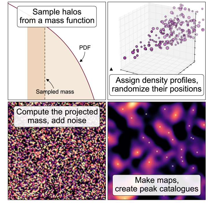
Figure 10: Illustration of our peak count model from creating fast simulations of uncorrelated halos. From LKS16.

Fig. 10 illustrates how we generate our peak count model. First, for a given redshift $z$, halo masses $M$ are randomly drawn from a halo mass function $n(M,z)$, for which we choose the fitting formula from 2001MNRAS.321..372J. The corresponding halos are placed in a comoving volume of given field of view, where the positions $x$ and $y$ perpendicular to the line of sigh are uniformly drawn. Halo profiles are attributed to the halos, in our case the NFW profile following NFW, asssuming the relation between mass and concentration from [2002MNRAS.337..875T]. Since there is no spatial correlation between halos due to the randomization of their positions, this corresponds to the 1-halo term in the halo model, see for a review [2002PhR...372....1C]. Next, lensing convergence and shear are computed for a given source galaxy redshift distribution, by adding up the contribution of all halos along the line of sight to a given soure galaxy redshift. Shape noise is added, if desired the convergence is computed from the shear, and peaks are counted in the final $\kappa$ map. We characterize the number of peaks with a histogram of the peak number probability function (pdf), also peak abundance, or peak function, as function of peak signal to noise ratio $\nu$. Alternatively, we also compute the cumulative pdf (cdf) following [2010MNRAS.402.1049D] and characterize the peak counts with the SNR at given percentiles of the cdf.

Our model makes two main assumptions: First, we claim that diffuse, unbound matter, for example in the form of filaments between halos, does not significantly contribute to the number of weak-lensing peaks. Similarly, structures such as voids are not simulated in our model. Note that models based on the halo model make the same assumptions. Second, we neglect spatial correlations between halos. Previous work has shown that correlated structure along the line of sight influences the number of peaks by only a few percent [2010ApJ...709..286M]. Note that in our model for a given line of sight more than one halo can contribute to the lensing signal, but in the form of random, uncorrelated halos.

We test the two hypotheses in LK15a by comparing our model predictions to $N$-body simulations. First, we replace all detected halos in the simulation by analytical NFW profiles, and remove all remaining dark-matter particles. This tests our first assumption (together with the universality of the NFW profile). Next, we randomize the $x$- and $y$-positions of all halos, testing our second assumption. The result is shown in Fig. 11. Our model agrees fairly well with the $N$-body simulation, although the error bars are large due to the small field of $53.7$ deg².

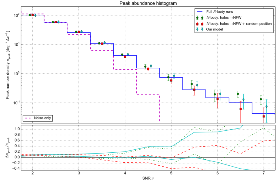
Figure 11: Peak counts from different outputs of an $N$-body simulation compared to our model. The blue curve shows the result from the full $N$-body simulation. For the green circles we have replaced halos with analytical NFW profiles. The green squares correspond to additionally randomized halo positions. The cyan diamonds are our model, independent of the simulation. The magenta line corresponds to peaks from noise-only maps. The upper panel shows the peak count histogram as function of peak SNR $\nu$; the lower plot shows the difference compared to the full $N$-body simulation (one standard deviation, where the errors are computed from different realisations of noise maps). From LK15a.

When replacing the $N$-body particles (blue curve) by NFW halos, the peak counts seem systematically lower (green circles). This might be due to the missing diffuse matter, or a decreased lensing strength of the NFW profiles compared to the simulated ones. For example, 2016arXiv161204041L showed that the number of peaks depends strongly on the concentration parameter.

We see a further decrease of peak counts when scrambling the halo positions (red squares), indicating the level of influence of correlated structures. Somewhat inbetween those two cases is our model, where we replace the simulated halo numbers and masses by our own draws from the mass function (cyan diamonds). Even though the number of halos in the simulation agrees well with the analytical mass function over a large range of redshift and mass [LK15a], the change of the number of peaks is visible. Ideally, in a cosmological analysis, one would account for the uncertainty in mass function, halo profiles, and mass-concentration relation, and marginalise over it.

The peak count model and data analysis software including parameter inference with Approximate Bayesian Computation (ABC, see Sect. 3.6) is available as the public software camelus [camelus_ascl].

A similar, stochastical model was proposed by 2009PhRvD..80l3020K. Our model extends this earlier work by simulating an entire field of view corresponding to a real survey. This allows us to include geometrical effects such as masking, boundary effects, PSF and other spatial systematic residuals, and finite-field effects due to the conversion from $\kappa$ to $\gamma$. We test some of these effects in LKS16 and LK17. The constraining power of peaks compared to the 2PCF was studied in PL17. In this paper we also demonstrated the agreement of our methods with the MICE-simulations [2015MNRAS.447.1319F], except for very high SNR $\nu$.

In on-going work, with PhD student Niall Jeffrey (advisor: Filipe Abdala) we examine fast approximate models such as PINOCCHIO [2002MNRAS.333..623T] to create a peak count model. This could be a middle way of running simulations that take significantly less time than a $N$-body simulation, but does contain spatial correlations between halos to some level.

3 Inference in cosmology

Much of my work has focused on how to obtain constraints on cosmological parameters from cosmic shear observations. To that end, I studied the necessary ingredients for cosmological analyses not only for weak lensing data, but for general problems in cosmology. This includes the covariance matrix (Sect. 3.1), the likelihood function (Sect .3.2, likelihood sampling techniques for parameter estimation (Sect. 3.3) and model comparison (Sect. 3.5), and likelihood-free inference methods (Sect. 3.6).

3.1 Covariance estimation

The covariance matrix of weak-lensing observables is an essential ingredient for cosmological analyses of cosmic shear data. Shear correlations at different scales are not independent but correlated with each other: The cosmic shear field is non-Gaussian, in particular on small scales, and different Fourier modes become correlated from the non-linear evolution of the density field. This mode-coupling leads to an information loss compared to the Gaussian case (unless higher-order statistics are included). If not taken into account properly, error bars on cosmological parameters will be underestimated.

Additionally, even in the Gaussian case Fourier modes are spread on a range of angular scales in real space, causing shear functions to be correlated across scales. The correlation strength depends on the filter function relating the power spectrum to the real-space observable (Sects. 2.1, 2.2). The broader the filter, the stronger is the mixing of scales, and the higher is the correlation.

For an observed data vector $\bm{d}=\{d_{i}\},i=1\ldots m$, the covariance matrix $\bm{\mathrm{C}}$ is defined as

$$C_{ij}=\langle\Delta d_{i}\Delta d_{j}\rangle=\langle d_{i}d_{j}\rangle-\langle d_{i}\rangle\langle d_{j}\rangle,$$ (45)

where the brackets denote ensemble average.

In a typical cosmic shear setting, the data vector $\bm{d}$ consists of functions of shear correlations (e.g. the shear two-point correlation function at $m$ angular scales $\theta_{i}$, or band-estimates of the convergence power spectrum $P_{\kappa}$ at $m$ Fourier wave bands with centres $\ell_{i}$). Those functions are quadratic in the observed galaxy ellipticity $\varepsilon$. The covariance then depends on fourth-order moments of $\varepsilon$. From (25), one can see that the covariance can be split into three terms: The shot noise, which is proportional to $\langle|\varepsilon^{\rm s}|^{2}\rangle^{2}=\sigma_{\varepsilon}^{4}$, and, in the absence of intrinsic galaxy alignment (Sect. 1.3.9), only contributes to the covariance diagonal; the cosmic variance term, which depends on fourth moments of the shear; and a mixed term.

In particular the cosmic variance term is difficult to estimate since it requires the knowledge of the non-Gaussian properties of the shear field.

3.1.1 The Gaussian approximation

The covariance of the convergence power spectrum $P_{\kappa}$ at an individual mode $\ell$ in the Gaussian approximation is the simple expression [1992ApJ...388..272K, 1998ApJ...498...26K, 2008A&A...477...43J]

$$\langle(\Delta P_{\kappa})^{2}\rangle(\ell)=\frac{1}{f_{\rm sky}(2\ell+1)}\left(\frac{\sigma_{\varepsilon}^{2}}{2\bar{n}}+P_{\kappa}(\ell)\right)^{2}.$$ (46)

Here, the survey observes a fraction of sky $f_{\rm sky}$, with a number density of lensing galaxies $\bar{n}$. The quadratic expression expands into shot-noise (first term), cosmic variance (second term), and a mixed term. In this Gaussian approximation, the fourth-order connected term of $\kappa$ is zero, and the cosmic variance consists of products of terms second-order in $\kappa$.

Analytical expressions for the Gaussian covariance of real-space second-order estimators have been obtained in [SvWKM02, KS04, 2009MNRAS.397..608S]. The power-spectrum covariance for shear tomography is easily computed [2004MNRAS.348..897T].

3.1.2 Non-Gaussian contributions

Equation (46) can be extended to the case of a non-Gaussian convergence field, with the next-leading terms depending on the trispectrum $T_{\kappa}$ [1999ApJ...527....1S, 2004MNRAS.348..897T]. Non-Gaussian evolution leads to a further coupling of small-scale modes with long wavelength modes that are larger than the observed survey volume. These super-survey modes were first introduced as beat coupling in 2006MNRAS.371.1188H, and later modeled in the halo model framework as halo sample variance 2009ApJ…701..945S,2013MNRAS.429..344KHSV;. Contrary to the other terms of the covariance that scale inversely with the survey area $f_{\rm sky}$, the super-survey covariance decreases faster. Therefore it is important for small survey areas [2009ApJ...701..945S, 2013PhRvD..87l3504T].

An alternative, non-analytic path is replacing the ensemble average in (45) by spatial averaging, and to estimate the covariance matrix from a large enough number $n$ of independent $N$-body simulations. To compute the inverse of this estimator, which is needed in the likelihood function (see following section), the dimension of the data vector $m$ has to be smaller than $n$ [andersen03, HSS07]. To reach percent-level precision for the inverse, $n$ has be much larger than $m$, which for future surveys with many tomographic bins means that the number of required simulations will be at least a few times $10^{4}$ [2013MNRAS.tmp.1312T, 2013PhRvD..88f3537D]. This was the path we chose for CFHTLenS tomography [CFHTLenS-2pt-tomo, CFHTLenS-mod-grav, CFHTLenS-IA] and higher-order statistics [CFHTLenS-2+3pt], and COSMOS [SHJKS09].

3.2 The likelihood function

To compare weak-lensing observations to theoretical predictions, one invokes a likelihood function $L$ as the probability of the observed data $\bm{d}$ of length $m$ given a model $M$ with a set of parameters $\bm{p}$ of dimension $n$.

For simplicity, in most cases, the likelihood function is modeled as an $m$-dimensional multi-variate Gaussian distribution,

$$L(\bm{d}|\bm{p},M)=(2\pi)^{-m/2}|\bm{\mathrm{C}}(\bm{p},M)|^{-1/2}\exp\left[-\frac{1}{2}\left(\bm{d}-\bm{y}(\bm{p},M)\right)^{\rm t}\bm{\mathrm{C}}^{-1}(\bm{p},M)\left(\bm{d}-\bm{y}(\bm{p},M)\right)\right].$$ (47)

The function $\bm{y}$ is the model prediction for the data $\bm{d}$, and depends on the model $M$ and parameter vector $\bm{p}$. This is only an approximation to the true likelihood function, which is unknown, since shear correlations are non-linear functions of the shear field, which itself is not Gaussian, in particular on small scales.

The true likelihood function can be estimated by sampling the distribution using a suite of $N$-body simulations for various cosmological parameters. Because of the high computation time, this has been done only for a restricted region in parameter space [2009A&A...504..689H, 2009A&A...505..969P, 2011ApJ...742...15T]. For weak-lensing peak counts (Sect. 2.3.3), using our fast simulations [LK15a], we have sampled the true likelihood function and compared this to the Gaussian and the copula likelihood [LK15b]. The copula is defined by transformed variables for which all one-dimensional pdfs are Gaussian. This makes the multi-variate likelihood function more Gaussian, but does not guarantee it [2011PhRvD..83b3501S].

The log-likelihood function can be approximated by a quadratic form, which is the inverse parameter covariance at the maximum point, called the Fisher matrix [KS69, TTH97]. The Fisher matrix has become a standard tool to quickly assess the performance of planned surveys, or to explore the feasibility of constraining new cosmological models, e.g. [DETF]. However, one has to keep in mind that the Fisher matrix is often ill-conditioned, in particular in the presence of strong parameter degeneracies, and its inversion requires a very high precision calculating of theoretical cosmological quantities, as we have shown in WKWG12.

In most cases, the parameter-dependence of the covariance in (47) is neglected, since the compuation of the covariance is very time-consuming, e.g. when derived from $N$-body simulations. When estimated from the data themselves, the cosmology-dependence of the covariance is missing altogether. This is a good approximation, as was shown in 2009A&A…502..721E and confirmed in CFHTLenS-2pt-notomo, in particular when only a small region in parameter space is relevant, for example in the presence of prior information from other cosmological data.

3.3 Parameter estimation

Theoretical models of cosmic shear observables can depend on a large number of parameters. Apart from cosmological parameters, a number of additional, nuisance parameters might be included to characterize systematics, calibration steps, astrophysical contaminants such as intrinsic alignment, photometric redshift uncertainties, etc. The number of such additional parameters can get very large very quickly and reach of the order a few hundred or even thousands, for example if nuisance parameters are added for each redshift bin [2008arXiv0808.3400B].

When inferring parameter constraints within the framework of a given cosmological model, one usually wants to estimate the probability of the parameter vector $\bm{p}$ given the data $\bm{d}$ and model $M$. In a Bayesian framework, this is the posterior probability $\pi$, which is given via Bayes’ theorem as

$$\pi(\bm{p}|\bm{d},M)=\frac{L(\bm{d}|\bm{p},M)P(\bm{p}|M)}{E(\bm{d}|M)},$$ (48)

which links the posterior to the likelihood function (see previous section) via the prior $P$ and the evidence $E$. In most cases, one wants to calculate integrals over the posterior, for example to obtain the mean parameter vector, its variance, or confidence regions. Such integrals can be written in general as

$$I(h)=\int{\rm d}^{n}p\,h(\bm{p})\pi(\bm{p}|\bm{d},M),$$ (49)

where $h$ is a function of the parameter $\bm{p}$. To calculate the mean of the $\alpha^{\rm th}$ parameter, $I(h)=\bar{p}_{\alpha}$, $h(\bm{p})=p_{\alpha}$. For the variance of $p_{\alpha}$, set $h(\bm{p})=(p_{\alpha}-\bar{p}_{\alpha})^{2}$. For a confidence region ${\cal C}$ (e.g. the 68% region around the maximum) $h$ is the characteristic function $1_{\cal C}$ of the set ${\cal C}$, that is $h(\bm{p})=1$ if $\bm{p}$ is in $\cal C$, and 0 else. Note that this does not uniquely define ${\cal C}$; there are indeed many different ways to define confidence regions.

In high dimensions, such integrals are most efficiently obtained by means of Monte-Carlo integration, in which random points are sampled from the posterior density function. Many different methods exist and have been applied in astrophysics and cosmology, such as Monte-Carlo Markov Chain (MCMC; cosmomc *cosmomc), Population Monte Carlo (see Sect. 3.4), or multi-nested sampling [2008MNRAS.384..449F]. Monte-Carlo sampling allows for very fast marginalization, for example over nuisance parameters, and projection onto lower dimensions, e.g. to produce 1D and 2D marginal posterior constraints.

MCMC provides a chain of $N$ points $\bm{p}_{j}$, which under certain conditions represent a sample from the posterior distribution $\pi$. Using this Markov chain, integrals of the form (49) can be estimated as sums over the $N$ sample points $\bm{p}_{j}$,

$$\hat{I}(h)=\frac{1}{N}\sum_{j=1}^{N}h(\bm{p}_{j}).$$ (50)

One caveat of this estimator is that in general, the samples are actually drawn from $L(\bm{d}|\bm{p},M)P(\bm{p}|M)$, or from the unnormalised posterior. It turns out not to be trivial to estimate the normalisation (evidence) $E$ with MCMC. However, the evidence drops out when using as MCMC method the very popular Metropolis-Hasting accept-reject algorithm [Metropolis53, Hastings70]. To get to the next step in the Markov Chain $\bm{p}_{i+1}$ from a previous position $\bm{p}_{i}$, only ratios of the posterior $\pi(\bm{p}_{i+1}|\bm{d},M)/\pi(\bm{p}_{i}|\bm{d},M)$ are involved. Thus, (50) can be obtained without the need to compute the parameter-independent normalisation.

Other Monte-Carlo sampling techniques might provide samples under a different distribution, and (50) has to be modified accordingly, see for example the following section with the case of PMC.

Alternatively, in a frequentist framework, one can minimize the function $\chi^{2}=-2\ln L$. Marginalisation can be performed with the so-called profile likelihood method [2014A&A...566A..54P]. Frequentist minimisation is equivalent to Bayesian inference with flat priors on all parameters.

Cosmic shear using current data is sensitive to only a few cosmological parameters, in particular $\Omega_{\rm m}$ and $\sigma_{8}$. Shear tomography is beginning to obtain interesting results on other parameters such as $\Omega_{K}$, or $w$. For parameters that are not well constrained by the data, for example $\Omega_{\rm b}$ or $h$, the (marginal) posterior is basically given by the prior density. Therefore, the prior should be chosen wide enough to not restrict other parameters, and to not result in overly optimistic constraints.

3.4 Population Monte Carlo (PMC)

In WK09 and KWR10 we develop for cosmology Population Monte Carlo, a sampling technique based on iterative importance sampling [cappe:douc:guillin:marin:robert:2007, CGMR03]. Importance sampling provides samples under a posterior distribution $\pi$, but samples from a different distribution, the so-called proposal or importance function $q$, choosen to be a simple function from where samples can be generated easily.

To provide samples under $\pi$, we re-write (49) as

$$I(h)=\int{\rm d}^{n}p\,h(\bm{p})\pi(\bm{p}|\bm{d},M)=\int{\rm d}^{n}p\,h(\bm{p})\frac{\pi(\bm{p}|\bm{d},M)}{q(\bm{p})}q(\bm{p}).$$ (51)

This identity holds for any $q$ whose support includes the support of $\pi$, and for functions $h$ whose expectation $I(h)$ is finite.

This expression is estimated by sampling under the proposal $q$. The Monte-Carlo estimator (50) is simply modified to account for the additional term in the integral,

$$\hat{I}(h)=\frac{1}{N}\sum_{j=1}^{N}h(\bm{p}_{j})w_{j};\qquad w_{j}=\frac{\pi(\bm{p}_{j}|\bm{d},M)}{q(\bm{p}_{j})}.$$ (52)

The $w_{j}$ are called importance importance weights.

To estimate the unnormalised posterior (52), can be modified to include the self-normalised importance ratios

$$\hat{I}(h)=\frac{1}{N}\sum_{j=1}^{N}h(\bm{p}_{j})\bar{w}_{j};\quad\bar{w}^{t}_{j}=\frac{w^{t}_{j}}{\sum_{i=1}^{N}\bar{w}^{t}_{i}},$$ (53)

where the $\bar{w}_{j}^{t}$ are the normalised importance weights. This circumvents the necessity to compute the normalisation $E$. Contrary to the case of MCMC however, PMC does provide a robust estimate of the evidence that comes at no extra cost, as I will show below.

The performance of importance sampling depends strongly on the choice of $q$. If the importance function does not well match $\pi$, many sampled points receive a very low weight, leading to a very poor efficiency and large variance of the estimator. PMC proposes to solve this problem by iteratively adapting the importance function to the posterior: A sequence of importance functions $q^{t},t=1\ldots T$ aims to approximate the target $\pi$.

The approximation is quantified by the Kullback-Leibler divergence, or relative entropy $K$,

$$K(\pi\|q^{t})=\int{\rm d}^{n}p\,\log\left(\frac{\pi(\bm{p}|\bm{d},M)}{q^{t}(\bm{p})}\right)\pi(\bm{p}),$$ (54)

which is an asymmetric measure of the similarity between two distributions. If $K$ is $0$, the two distributions are identical almost everywhere, whereas for $K\rightarrow 1$, $\pi$ and $q$ are very different.

The PMC algorithm adjusts the density $q^{t}$ incrementally such that the divergence decreases with progressive iterations, or $K(\pi\|q^{t+1})<K(\pi\|q^{t})$.

Following cappe:douc:guillin:marin:robert:2007, we use a variant of the expectation-maximization (EM) algorithm to obtain updated parameters that determine the proposal function, for which we choose a mixture (weighted sum) of Gaussian or Student-t distributions. The parameters are mixture weights, mean, and covariance matrix for the Gaussian or Student-t components of the mixture model. cappe:douc:guillin:marin:robert:2007 derived closed-form solutions for these parameters, which are given as integrals over the posterior $\pi$. In iteration $t+1$, these integrals are approximated by evaluating their importance sampling estimator using the samples and importance weights from the previous iteration $t$. The details of the algorithm are summarized in WK09.

3.4.1 Convergence and effective sample size

Formally, there is no convergence criterium for PMC. Eq. (53) is an unbiased estimator of $I(h)$ if the support of the proposal $q$ covers $\pi$. Unlike the case of MCMC, there is no burn-in phase and no asymptotic convergence of the chain towards the postieror distribution. However, for a badly adapted proposal, the estimate might be very noisy. Therefore, a criterium is introduced that monitors the improvement of the adaption. An estimate of $\exp(-K)$ is the so-called normalised perplexity for iteration $t$, $p^{t}$,

$$p^{t}=\exp(H^{t}/N),$$ (55)

where $H^{t}$ is the Shannon entropy of the normalised weights,

$$H^{t}=-\sum_{j=1}^{N}\bar{w}^{t}_{j}\log\bar{w}^{t}_{j}.$$ (56)

The perplexity ranges between $0$ and $1$. Values of $p$ close to unity indicate good agreement between the importance function and the posterior.

A stopping criterium for a PMC run can be defined to be the iteration for which $p$ exceeds a pre-determined threshold. Typically, a final importance run with a higher number of sample points than for each previous iteration is being carried out using the proposal from the last iteration. This will be the final sample use for inference, to estimate (53).

A quantity related to the efficiency of PMC is the effective sample size, ESS^t,

$$\mathrm{ESS}^{t}=\left(\sum_{j=1}^{N}\left\{\bar{w}_{j}^{t}\right\}^{2}\right)^{-1},$$ (57)

where $1\leq\mathrm{ESS}^{t}\leq N$. The effective sample size can be interpreted as the number of sample points with non-zero weight. The ESS can directly be compared with the number of sampled points of a Markoc Chain multiplied with the acceptance rate.

3.4.2 Performance

Fig. 12 shows perplexity and effective sample size as number of sample points, for a PMC run using CMB anisotropy data from WMAP5 [WMAP5-Hsinshaw08]. We sample seven cosmological parameters of a $w$CDM model, see WK09 for details. PMC is run for $10$ iterations, using a mixture Gaussian importance function. Each point on the figure shows the value after the corresponding iteration. Each of the first $9$ iterations is performed with $10,000$ sample points, except for the final one, which has a number five times larger, to reduce Monte-Carlo noise.

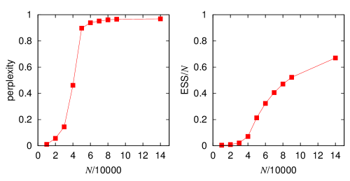
Figure 12: Perplexity (left panel; eq. (55)) and effective sample size ESS divided by the number of sample points, ESS/$N$ (right panel; eq. (57)), as a function of the cumulative sample size $N$. The likelihood is WMAP5 for a flat $\Lambda$CDM model with six parameters. From WK09.

After five iterations, or $50,000$ sampled points, the perplexity reaches values of $0.9$ and higher. The normalised ESS increases up to the last iteration and exceeds $0.6$. This is much higher than the typical MCMC acceptance rate ot $0.25$, even when taking into account the number of samples from all iterations ($130,000$ in total).

The number of samples needed for PMC is of the same order of magnitude as for MCMC. The total computing time is therefore similar. However, importance sampling separates the (typically time-consuming) evaluation of the posterior, or the likelihood function, from the sampling. Obtaining the sample points (= draws from Gaussian or Student-t distributions) for each iteration is very fast. The computation of the importance weights, which involves evaluation of the likelihood at the sampled points, can then be performed in parallel. For a number $n$ of CPUs, the wall-clock time gain is nearly $n$.

In WK09 we show for a toy example in 10 dimension that PMC is capable to well sample the tails of a narrow distribution. The variance of the estimator (53) for various functions $h$ such as the mean and credible regions is typically smaller than for MCMC.

The implementation of Population Monte-Carlo for cosmology is available as the public software CosmoPMC [cosmo_pmc_ascl].

3.5 Model selection

The previous section discussed estimating parameters within a given cosmological model, with the goal to measure mean and error bars of model parameters. Taking one step back, one can ask the more fundamental question what the best model is that describes the observations. This is a qualitative different step and needs to compare different models, which is independent of estimating parameters of those models. Such a comparison has to account for the ability of models to describe the data, and the model complexity. This is achieved naturally with posterior probabilities from a Bayesian analysis.

The Bayesian evidence $E$ is the denominator in Bayes’ theorem (48). Since the posterior, being a probability distribution function, is normalised, this normalization is identical to $E$. Re-writing (48) and integrating yields the evidence as the integral over the unnormalised posterior (likelihood $\times$ prior)

$$E(\bm{d}|M)\int{\rm d}^{n}p\,\pi(\bm{p}|\bm{d},M)=E(\bm{d}|M)=\int{\rm d}^{n}p\,L(\bm{d}|\bm{p},M)P(\bm{p}|M).$$ (58)

This integral over the entire parameter space can be interpreted as a measure of the overall model probability $M$ given the data $\bm{d}$.

The likelihood $L$ accounts for the goodness of the fit with respect to the data, quantifying the data fidelity of the model. The better the agreement of the data with the model, the higher the likelihood and thus the larger $E$ will be.

The Bayesian evidence also crucially depends on the prior $P$. The larger the parameter space, the smaller the amplitude of $P$ will be in general, since $P$ is a normalised probability distribution, and thus the smaller the evidence becomes. This penalizes models that have a large parameter space, and that are thus not very predictive: The predictability of a model $M$ given some data $\bm{d}$ only makes sense when compared to a prior knowledge. A model has low predictability if it requires fine-tuning of parameters, i.e. when the posterior is very concentrated compared to the prior.

A good model is one for which the prior distribution of parameters closely matches “reality”, that is the posterior distribution obtained from a measurement $\bm{d}$. This is true in particular when the prior is obtained from first principles or physical knowledge of the system in question. To use the Bayesian evidence as model probabilty, this needs to be the case, since the prior is an integral part of the model, and thus has to be physically well-motivated instead of choosen in an ad-hoc way [2008MNRAS.388.1314E]. For arbitrary priors, the results of Bayesian model comparison are arbitrary.

The Bayesian evidence has thus a built-in Occam’s razor term, penalizing models with high complexity (in the form of having many additional parameters, or a large, “wasted” parameter space), see also berger:jefferys:1992 and mackay:2002.

To compare two models $M_{1}$ and $M_{2}$, we use the Bayes factor [jeffreys:1939],

$$B_{12}=\frac{E_{1}}{E_{2}}:=\frac{E(\bm{d}|M_{1})}{E(\bm{d}|M_{2})}.$$ (59)

If $B_{12}$ is larger (smaller) than unity, the data favour model $M_{1}$ ($M_{2}$) over the alternative model. To quantify the “strength of evidence” contained in the data, jeffreys:1961 introduced an empirical scale, see Table 1. This is only a rough guideline for decision making and of course the proposed boundaries are mostly subjective, albeit connected with information theory. I refer the reader to 2008ConPh..49…71T for a pedagogical review about the Bayesian evidence and its use for model comparison.

Table 1: Jeffrey’s scale to quantify the ‘strength of evidence’ for a corresponding range of the Bayes factor $B_{12}$ in (59), assuming $B_{12}>1$.

$\ln B_{12}$	$B_{12}$	Strength
$<1$	$<2.7$	Inconclusive
$1\ldots 2.5$	$2.7\ldots 12$	Weak
$2.5\ldots 5$	$12\ldots 150$	Moderate
$>5$	$>150$	Strong

The integral (58) is readily approximated with the importance sampling estimator (52), where the function $h$ is unity,

$$\hat{E}(\bm{d},M)=\frac{1}{N}\sum_{j=1}^{N}w_{j}.$$ (60)

Note that here the unnormalised importance weights are used.

Below I show an example from KWR10, comparing inflatonary models of the power spectrum of primordial perturbations. I use data from CMB anisotropies (WMAP5-Hsinshaw08 *WMAP5-Hsinshaw08), SNIa (kowalski-2008 *kowalski-2008) and BAO (2005ApJ…633..560E *2005ApJ…633..560E).

I model the primordial scalar perturbations power spectrum as

$$P_{\delta}(k)\propto k^{n_{\rm s}+\frac{1}{2}\,\alpha_{\rm s}\ln(k/k_{0})},$$ (61)

with the parameters $n_{\rm s}$ being the scalar spectral index, and $\alpha_{\rm s}$ the “running” of the index. The pivot scale $k_{0}$ is fixed to $k_{0}=0.002$ Mpc^-1. In addition, tensor modes (gravitational waves) have the power spectrum

$$P_{\rm t}(k)\propto k^{n_{\rm t}},$$ (62)

with tensor spectral index $n_{\rm t}$. The ratio between tensor and scalar perturbation spectra at scale $k_{0}$ is denoted by $r$.

The standard $\Lambda$CDM model $M_{2}$ has $\alpha_{\rm s}=n_{\rm t}=r=0$, with only $n_{\rm s}$ being a free parameter. Against $M_{2}$ we test various models $M_{1}$, where we keep combinations of $\alpha_{\rm s}$ and $r$ free. The tensor index $n_{\rm t}$ is unconstrained by current data and therefore not included. In addition, we test the Harrison-Zel’dovich model of a scale-free power spectrum with $n_{\rm s}$. This model has meanwhile been ruled out at the $5\sigma$ level by Planck [2015arXiv150201589P] for the standard $\Lambda$CDM model, but this significance decreases for extended models.

To obtain physically motivated priors on the power-spectrum parameter, we consider the slow-roll approximation of inflation. This approximation provides an infinite hierarchy of flow equations describing the dynamics of the single scalar field which drives inflation [2006JCAP...07..002P]. The slow-roll parameters to first order are $\varepsilon$ and $\eta$, which are given in terms of the inflaton potential and Hubble parameter during inflation.

Slow-roll conditions are satisfied when $0\leq\varepsilon\leq 0.1$ and $|\eta|\leq 0.1$. Although the numerical values are approximate, they are natural limits for the validity of the Taylor-expansion of the power spectrum $P(k)$ in $\ln(k/k_{0})$, see 2006JCAP…08..009M. From these limits, and their relations to the power-spectrum parameters we derive priors on the latter, see Table 2. We choose uninformative (flat) priors for simplicity. With that we have the ingredients for a meaningful Bayesian model comparison analysis, which are well-defined models with physically motivated priors.

Table 2: Prior ranges for primordial model comparison. The prior ranges for primordial parameters are derived from the slow-roll approximation.

Parameter	Description	Min.	Max.
$n_{\rm s}$	Scalar spectral index	0.39	1.2
$\alpha_{\rm s}$	Running of spectral index	-0.2	0.033
$r$ (lin. prior)	Tensor-to-scalar ratio	0	1.65
$\ln r$ (log. prior)	Tensor-to-scalar ratio	-80	0.50

In Fig. 13 we show the Bayes factor of various models $M_{1}$ with respect to the standard, reference model $M_{2}$ (the flat $\Lambda$CDM universe with $n_{\rm s}=\mbox{const}$), as function of the number of parameters $n_{\rm par}$ for each model $M_{1}$. A running spectral index is favoured weakly, all other cases are disfavoured. The evidence against the Harrison-Zel’dovich model ($n_{\rm s}=1$) is only weak, even though the measured value of $n_{\rm s}=0.9622\pm 0.0145$ is inconsistent with unity at the $2.6\sigma$ level for this data set. This shows the importance of Bayesian model comparison when compared to the significance of marginalised error bars using a single model, when making statements about ruling out models.

Tensor perturbations are moderately disfavoured. However, as example of the influence of the prior choice, we use in addition a model with a flat prior in $\ln r$ instead of $r$. As lower limit we choose $-80$, corresponding to the energy scale of Big Bang Nucleosynthesis as a conservative lower limit of the inflation energy scale (2006PhRvD..73l3523P *2006PhRvD..73l3523P). The large prior of the logarithmic tensor-to-scalar ratio causes this model to be strongly disfavoured.

Figure 13: Ratio of evidences, or Bayes factor, for various models ${M}_{1}$ with respect to the reference model ${M}_{2}$, a flat $\Lambda$CDM universe with constant $n_{\rm s}$. From KWR10.

3.6 Approximate Bayesian Computation (ABC)

Approximate Bayesian Computation [2011arXiv1101.0955M, 2012MNRAS.425...44C] is a so-called likelihood-free statistical inference method. That means the evaluation of a likelihood function is bypassed to obtain samples from the posterior distribution $\pi$. ABC allows to do parameter inference in cases where the likelihood function is unknown, or too expensive (time-consuming) to evaluate. It is thus ideal for non-Gaussian observables, where the approximation of a multi-variate Gaussian for the likelihood might be inappropriate. ABC allows us to test this assumption.

The requisite for ABC is a stochastical process that provides simulated realisations $\{\bm{x}_{i}\}$ of the data $\bm{d}$ for a given parameter $\bm{p}$ and model class $M$. These simulations are the model prediction for that parameter; the model is here not a single, deterministic vector $\bm{y}(\bm{p}|M)$ as before, but a stochastic random variable drawn from a distribution.

ABC requires that this distribution is the true underlying probability distribution, or likelihood $L$, of the observable $\bm{d}$. Then, the simulations $\bm{x}_{i}$ are a sample under $L$, and the density of the sample points represent an estimate of $L$ of a given parameter $\bm{p}$ and model $M$. For parameter inference, we need to know the probability of the data, $L(\bm{d}|\bm{p},M)$ given $\bm{p}$ and $M$. that we observed $\bm{d}$. How do we get this probabilty without calculating $L(\bm{d})$?

This is best illustrated for discrete data: If we have $N$ model prediction realisations $\{\bm{x}_{i}\}$ for a parameter $p$ of some discrete data $\bm{d}$, the probability of observing $\bm{d}$ is the number of realisations $r$ for which $\bm{x}_{i}=\bm{d}$, divided by $N$. Interestingly, this is a frequentist interpretation of probability, which is the number of matches over the total number of events.

We can write this relative frequency of matches as sum over the distribution (the likelihood $L$) of $\bm{x}_{i}$ times the Kronecker delta to only select matches. If in addition the parameter $\bm{p}$ is drawn from the prior distribution $P(\bm{p}|M)$, the the distribution of matching events, which we call $\hat{\pi}_{\rm ABC}$, is

$$\hat{\pi}_{\rm ABC}(\bm{p}|\bm{d},M):=\sum_{i=1}^{N}L(\bm{x}_{i}|\bm{p},M)P(\bm{p}|M)\delta_{\bm{x}_{i},\bm{d}}=L(\bm{d}|\bm{p},M)P(\bm{p}|M).$$ (63)

This justifies thus the use of the symbol $\pi$, since the result is an unbiased estimator of the (unnormalised) posterior of $\bm{p}$!

An additional step is performed with ABC: The number of realisations $N$ can be as small as one. This might sound surprising at first, since a single realisation $\bm{x}$ is not likely to match $\bm{d}$, so $\hat{\pi}_{\rm ABC}$ can be zero. But the probability of a match is equal to $L(\bm{x}|\bm{p},M)$, independent of the number of realizations $N$, so the expectation value of (63) is still an unbiased estimator of $\pi$ even for $N=1$. The large variance of this one-sample estimator is compensated by the large number of sampled parameters $\bm{p}$ that are typically explored in sampling of the posterior. It turns out that the overall sampling (or Monte-Carlo) noise does not increase for $N=1$. This one-sample test leads to an accept-reject algorithm.

The application of ABC to continuous data requires further adaptations. Since strict equality between two continuous variables are practically not possible, sampled points $\bm{x}_{i}$ are accepted when they fall within some tolerance level $\varepsilon$ of $\bm{d}$. For multi-variate data, this also requires a metric $D$ that can be compared to $\varepsilon$. In addition, the complexity of high-dimensional data is typically reduced to a lower-dimensional space using a summary statistic $\bm{s}$ of the data. Thus, a model $\bm{x}$ is accepted if

$$D[\bm{s}(\bm{d}),\bm{s}(\bm{x})]<\varepsilon;\quad\mbox{or equivalently}\quad\bm{x}\in{\cal D}_{\varepsilon}[\bm{s}(\bm{d})],$$ (64)

where ${\cal D}_{\varepsilon}(\bm{z})$ is the $q$-dimensional ball with radius $\varepsilon$ centred on $\bm{z}$.

The accepted points follow a distribution that is a modified version of (63),

$$\pi_{{\rm ABC},\varepsilon}(\bm{p}|\bm{d},M)=L_{\varepsilon}(\bm{d}|\bm{p},M)P(\bm{p}|M),$$ (65)

where $L_{\varepsilon}(\bm{d}|M)$ is the probability that a proposed parameter $\bm{p}$ passes the one-sample tolerance test (64),

$$L_{\varepsilon}(\bm{d}|\bm{p},M)\equiv\int{\rm d}^{n}x\,L(\bm{x}|\bm{p},M)\mathbf{1}_{{\cal D}_{\varepsilon}[\bm{s}(\bm{d})]}[\bm{s}(\bm{x})].$$ (66)

The sum over discrete events $\bm{x}_{i}$ is now an integral over models, and the Kronecker delta has been replaced with the indicator function $\mathbf{1}_{A}(\bm{x})$, which is unity if $\bm{x}\in A$, and zero otherwise. This accept-reject algorithm is illustrated in Fig. 14.

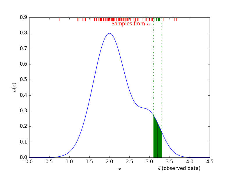
Figure 14: Illustration of the ABC accept-reject method in one dimension. Sample points (with positions indicated at the top) are sampled from the underlying likelihood function $L$ of some observable $x$. The observed data point marked at $d$. We want to obtain the likelihood function at the position of the data, $L(x=d)$. A Monte-Carlo estimate of $L(d)$ is given by the density of sample points at $d$. ABC approximates this density by defining a tolerance $\varepsilon$ around $d$, and counting the number of points within this limit, normalised by the total number of samples. In a one-sample test limit, this frequency is the acceptance probability, which is equal to the green area divided by the total area under the $L$ curve.

The main assumption of ABC is now that the probability distribution function (66) is a good approximation of the true, underlying likelihood function $L$ of the data $\bm{d}$,

$$L_{\varepsilon}(\bm{d}|\bm{p},M)\approx L(\bm{d}|\bm{p},M).$$ (67)

and consequently the ABC posterior (65) an approximation of the true posterior $\pi$.

This assumption relies on the three ingredients for ABC sampling: the summary statistic $\bm{s}$, the distance function $D$, and the tolerance $\varepsilon$. Note that traditional Monte-Carlo likelihood sampling approaches also depend on the choice of a summary statistic: In most cases the size of the observed data $\bm{d}$ is huge (e.g. CMB pixelised maps or time series, weak-lensing galaxy shape catalogues, SNIa lightcurve time measurements), and is typically reduced to a much smaller observable (e.g. power spectrum, correlation function, magnitude + stretch + color), by a mapping $\bm{s}(\bm{d})$.

McKinley09 showed that the choice of a summary statistic and distance function are of great importance for the ABC performance. In LK15b we only used one summary statistic, namely $\bm{s}(\bm{x})=\bm{x}$, where $\bm{x}$ is the (already reduced) data vector. In our case of weak-lensing peak counts (Sect. 2.3.3), $\bm{x}$ was chosen to be the number of peaks $\bm{n}=(n_{1},n_{2},\ldots)$ (peak abundance or pdf) as function of peak SNR $\nu_{i}$.

LKS16 compared two different distance functions $D$, which are the square root of scalar products of the two vectors $\bm{x}$ and $\bm{d}$. One distance, $D_{2}$, uses the full data covariance matrix to compute the scalar product, the other one, $D_{1}$, only weighs the data by the variance (diagonal of the covariance). Note that ABC with the distance $D_{1}$ does not necessarily neglect all correlation between data points — these are included automatically in the simulated model predictions under the joint, multi-variate likelihood function $L$. These correlations are only neglected under $D_{1}$ when deciding whether a model $\bm{x}$ for a parameter $\bm{p}$ is close enough to $\bm{d}$ for $\bm{p}$ to be accepted.

We found that $D_{1}$ and $D_{2}$ give very similar results when data points are weakly correlated, but $D_{1}$ provided overly tight constraints on parameters for highly correlated data, with under-estimation of the error of $\Sigma_{8}$ by 40%.

The tolerance $\varepsilon$ is best set in an iterative approach. This automatically solves the problem of fixing the tolerance a priori: If $\varepsilon$ is too large, too many points are accepted. In that case, $L_{\varepsilon}$ (66) approaches unity, and ABC effectively provides samples from the prior $P$. If $\varepsilon$ is too close to zero, so is $L_{\varepsilon}$, and sampling becomes very inefficient, with the overwhelming majority of points being rejected. In [LK15b] we use an iterative importance-sampling algorithm together with ABC. This sequential Monte-Carlo (SMC) ABC method has similarities with population Monte Carlo (Sect. 3.4), and is therefore also calles PMC ABC.

4 Measuring weak lensing

The cosmological interpretation of cosmic shear measurements requires the observation of large and deep sky areas in superb image quality, together with sophisticated image analysis methods. A significant detection of cosmic shear requires a very large number of galaxies to high redshifts (of order unity) and low signal-to-noise ratios (down to $10$ - $15$). The shapes of those faint galaxies have to be measured with high accuracy. Galaxy images have to be corrected for the point-spread function (PSF). The PSF is the combined effect of the imaging system consisting of the atmosphere (for ground-based surveys), telescope optics, and detector. To estimate the PSF, a very pure sample of stars, uncontaminated by small galaxies, has to be selected. Shape measurements typically have to be calibrated. To ensure measurement biases small enough compared to the statistical errors, large sets of realistic image simulations need to be used. In addition, the interpretation of shape correlations depends crucially on the redshift distribution of the lensed galaxy sample, see (21). Multiple optical band observations have to be used to estimate photometric redshifts. This section gives a brief overview of the methods for weak lensing measurements I have used in my work.

4.1 Galaxy shape measurement

The first family of shape measurement methods is moment-based direct estimation. One of the most widely used methods of this type is KSB (Kaiser, Squires & Broadhurst 1995). KSB measures ellipticity directly on an image using weighted second-order moments of the galaxy brightness distribution. The convolution of the image with the PSF is approximated by linear operations on the ellipticities; it is therefore a perturbative method. Alternatively, instead of correcting the ellipticities as in KSB, the PSF deconvolution can be done directly on the moments of the galaxy light distribution [2000ApJ...536...79R]. This is more rigorously explored by DEIMOS (deconvolution of image moments), a truncated hierarchy of higher-order moments in 2011MNRAS.412.1552M.

KSB was used in our cosmic-shear measurements [FSHK08, SHJKS09]. Deconvolution in moment space, inspired by DEIMOS, but using unweighted moments on denoised images, was one of my contributions to the GREAT3 challenge.

A second large family of shape measurement methods is based on model fitting. These indirect methods assume a model for the surface brightness $I$, including ellipticity parameters, and fit the model to the observed image. One of the advantages of such forward-fitting methods is the straightforward treatment of the PSF: The model is more easily and robustly convolved with the PSF than the observed (pixellised, noisy, maybe partially masked) image is deconvolved. A fully Bayesian forward-fitting method is lensfit, which measures the posterior distribution of ellipticity for galaxies on individual exposures, and combines the results in a Bayesian way without information loss [2007MNRAS.382..315M, 2008MNRAS.390..149K, CFHTLenS-shapes]. A further notable model-fitting method that I have used is gfit [2012arXiv1211.4847G]. lensfit turned out to be the superior method for CFHTLenS. gfit was used as main method by the CEA-EPFL team in the GREAT3 challenge, and is used in on-going work on shear calibration [pujol_shear_bias_17], and for the analysis of the Canada-France Imaging Survey (CFIS), see Sect. 6.1.

4.1.1 Shape measurement biases

One can make the very general statement that the non-linear dependence of ellipticity estimators on the light distribution in the presence of noise creates a bias, the so-called noise bias. This bias has been investigated for methods based on moments [2004MNRAS.353..529H] and model fitting [2012MNRAS.425.1951R, 2014MNRAS.441.2528K].

A further source of bias is related to incorrect assumptions about the light distribution, the so-called model bias [2010MNRAS.404..458V]. Not only model-fitting techniques, but also direct methods are still not free from such assumptions: For example, moment-based methods require weight functions whose profile and size should match the observed images, and in fact, direct and indirect methods show very similar biases related to galaxy morphology [pujol_shear_bias_17].

Shape biases can be characterised to first approximation by a multiplicative component $\bm{m}$, and and additive term $\bm{c}$. These bias parameters are given by the relation between observed and true ellipticity [2006MNRAS.366..101H, STEP1],

$$\varepsilon_{i}^{\rm obs}=(1+m_{i})\varepsilon_{i}^{\rm true}+c_{i};\quad i=1,2.$$ (68)

The shear biases $\bm{m}$ and $\bm{c}$ are generally functions of galaxy properties and redshift. Current shape measurement methods provide shear estimates with resudial (after calibration) $m$ at the $1$ to few percent level, and $c$ between $10^{-3}$ and $10^{-2}$. Typically, the calibration of measured shears is performed using large image simulations (Sect. 4.4). Recent work has been looking into calibration by using the data themselves, the so-called meta-calibration approach [2017arXiv170202600H, 2017ApJ...841...24S]. Future surveys require the accuracy of calibrated shapes to be on the order of $0.1$% [2006MNRAS.366..101H, 2013MNRAS.429..661M, 2013MNRAS.431.3103C], see Sect. 6.1.

4.2 PSF correction

To estimate the PSF at the position of a galaxy, one has to select stars on the image, measure their shape, and interpolate the resulting PSF to the position of the galaxy. This requires a sample of suitable stars, i.e. without saturated pixels, not hit by cosmic rays, and uncontaminated by galaxies. A common selection criteria is the identification of the stellar locus in a size-magnitude diagram. This is a region of bright and small objects that is relatively well isolated from resolved galaxies and unresolved, dim objects such as very faint galaxies and detection artefacts. Additionally, colour information can be added to classify stars and galaxies.

The PSF (in form of parameters, a pixellised vignette, or a high-resolution model), is then interpolated onto the galaxy position. For ground-based observations in the past, this has usually been done with a two-dimensional polynomial or a rational function. For mosaic multi-CCD cameras, discontinuities between chips are common and have to be accounted for in the PSF model, for example by performing fits on each chip individually [CFHTLenS-shapes].

4.3 Error modelling and residual systematics

Any weak lensing data analysis must be completed with a robust error modeling. This step is necessary to quantify any residual systematics caused by an imperfect PSF correction, since those residuals can mimic a cosmological signal.

4.3.1 Star-galaxy correlation

The most commonly used approach is a null test of the correlation between the stellar ellipticities $\varepsilon^{\star}$ (before PSF correction) and the corrected galaxy shapes $\varepsilon$. This star-galaxy ellipticity correlation function is defined as

$$\xi_{\rm sys}=\langle\varepsilon^{\star}\varepsilon\rangle.$$ (69)

Note that a non-zero signal on a small region on the sky could come from chance alignments between PSF pattern and a coherent shear from large-scale structure. To interpret measurements of $\xi_{\rm sys}$, this cosmic variance contribution needs to be accounted for [CFHTLenS-sys].

4.3.2 PSF model - residual correlation

Two correlation functions quantify the PSF model. These are the auto-correlation of the PSF residuals, $D_{1}$, and the cross-correlation between PSF and PSF residuals, $D_{2}$ [2010MNRAS.404..350R]. These two correlation functions are defined as

$$D_{1}(\theta) =\left\langle\left(\varepsilon-\varepsilon_{\rm m}\right)^{\ast}\left(\varepsilon-\varepsilon_{\rm m}\right)\right\rangle(\theta);$$

$$D_{2}(\theta) =\left\langle\varepsilon^{\ast}\left(\varepsilon-\varepsilon_{\rm m}\right)+\left(\varepsilon-\varepsilon_{\rm m}\right)^{\ast}\varepsilon\right\rangle(\theta).$$ (70)

Here, $\varepsilon$ is the observed ellipticity of a star, and $\varepsilon_{\rm m}$ the PSF model ellipticity. These functions do not only measure the amount of residuals $\left(\varepsilon-\varepsilon_{\rm m}\right)$, but the spatial correlation of residuals. This can be introduced by a PSF model that does not well represent the spatial variation of the PSF over the detector. In case of a perfect PSF model, both correlation functions are expected to vanish identically, $\langle D_{1}\rangle=\langle D_{2}\rangle=0$.

2010MNRAS.404..350R writes the observed ellipticity $\varepsilon$ of a galaxy as the sum of true ellipticity $\varepsilon_{\rm t}$ and noise $N$,

$$\varepsilon=\varepsilon_{\rm t}+N,$$ (71)

and the model ellipticity $\varepsilon_{\rm m}$ as sum of true ellipticity $\varepsilon_{\rm t}$ and model uncertainty $m$,

$$\varepsilon_{\rm m}=\varepsilon_{\rm t}+m.$$ (72)

The two correlation functions can then be written as

$$D_{1}(\theta) = -\left\langle m^{\ast}N+N^{\ast}m\right\rangle(\theta)+\left\langle m^{\ast}m\right\rangle(\theta);$$

$$D_{2}(\theta) = -\left\langle m^{\ast}N+N^{\ast}m\right\rangle(\theta)-\left\langle m^{\ast}\varepsilon_{\rm t}+\varepsilon_{\rm t}^{\ast}m\right\rangle(\theta).$$ (73)

In particular the second function $D_{2}$ is a useful diagnostic since it is negative definite. In case of over-fitting, the model tends to fit the noise rather the true ellipticity, which creates correlations between the noise $N$ and the model uncertainty $m$, and $D_{2}$ becomes significantly negative.

I illustrate such a case in Fig. 15. Non-zero $D_{1}$ and $D_{2}$ indicate PSF residual correlations, in particular on small scales, where the spatial PSF model, a bi-variate polynomial with varying degree, seems to not well fit data. The increasing negative $D_{2}$ with increasing polynomial degree shows cases of over-fitting for the more complex models, indicating that the true PSF variation shows less degrees of freedom.

A second example is discussed below in Sect. 4.4.1.

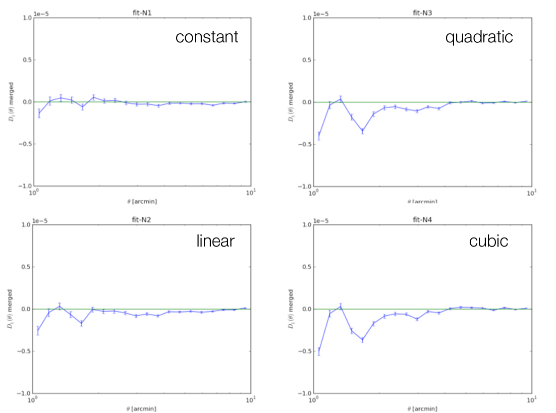
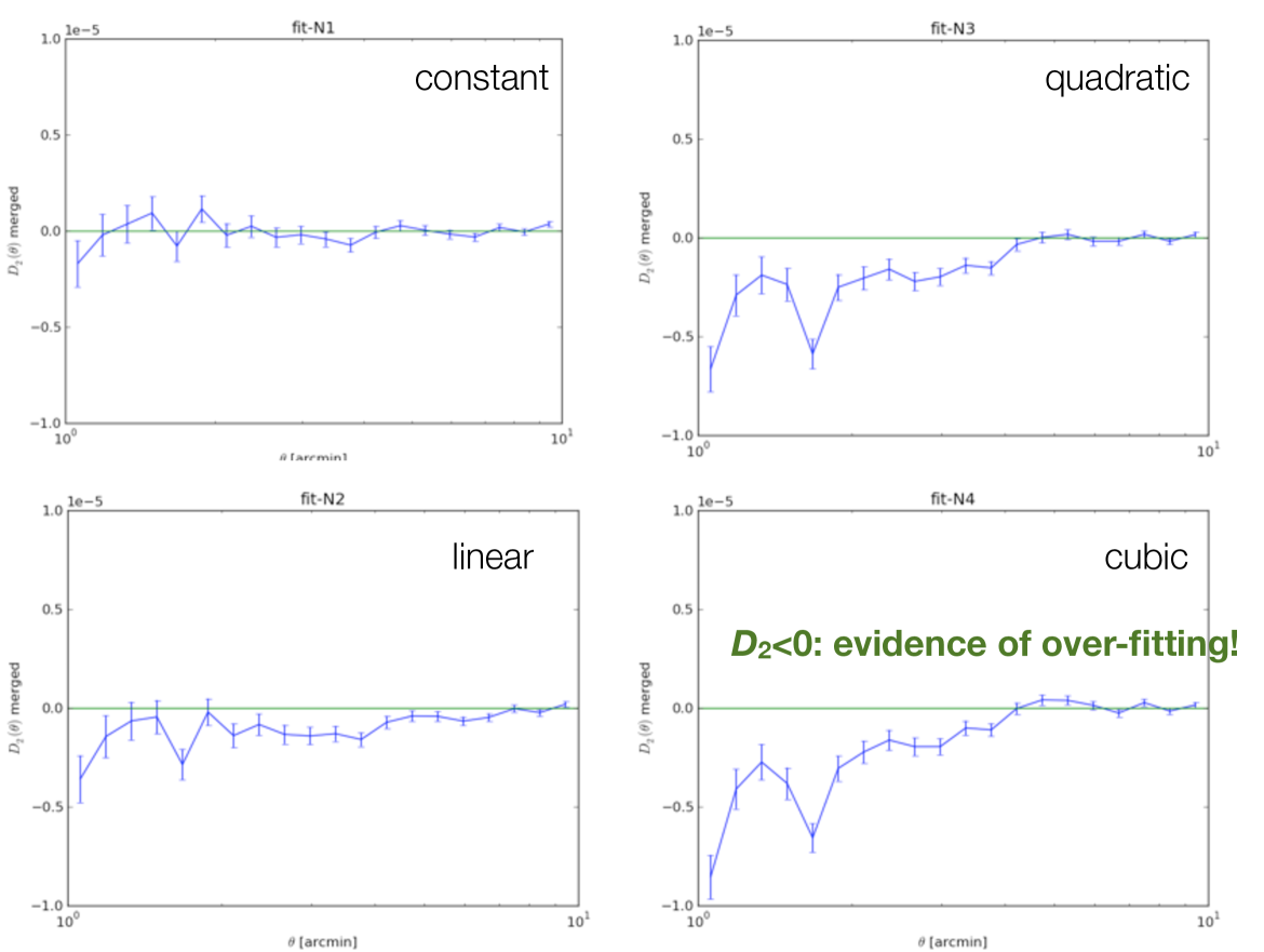
Figure 15: The PSF diagnostic correlation functions $D_{1}$ (upper four panels) and $D_{2}$ (lower four panels) as function of angular scale $\theta$, for the Dark Energy Survey (DES) data challenge #5 simulations. The four sub-panels show PSF polynomial models of increasing degree, from 0 (constant) to 3 (cubic). See Sect. 4.3.2.

.

4.4 Image simulations

Image simulations have been created as collaborative projects within the weak-lensing community, such as the Shear TEsting Project (STEP) with the two consecutive blind tests STEP1 [STEP1] and STEP2 [STEP2]. Public challenges like the GRavitational lEnsing Accuracy Testing (GREAT) projects have been launched to reach out to a larger community, in particular computer science, to invite more ideas to tackle the problem of galaxy shape measurement. This contains GREAT08 [2009AnApS...3....6B, 2010MNRAS.405.2044B], GREAT10 [2010arXiv1009.0779K, 2012MNRAS.423.3163K, Kitching:2012fj], and GREAT3 [2013arXiv1308.4982M].

Those collaborative image simulation projects typically started under simple, well-controlled conditions, for example, a constant PSF, constant shear over the field, and analytical galaxy light distributions with high signal-to-noise. They then progressed to more complex and more realistic images, for example galaxy images based on observed HST deep fields. The purpose of those simulations is to test estimates of shear with amplitudes of a few percent to an accuracy at also the percent level. This is typically quantified in terms of multiplicative and additive bias (68). The number of simulated images is necessarily very large, producing hundreds of gigabytes of data.

In the following sections, I briefly discuss some of my past work on galaxy shape measurement, bias quantification, and PSF modelling with image simulations.

4.4.1 GREAT10

Fig. 16 shows the PSF pattern of a GREAT10 star challenge image. Together with Bernhard Riedl, Diploma student under my and Jochen Weller’s supervision (Ludwigs-Maximilians-Universität München), we fit this pattern with bi-variate polynomials in the pixel coordinates $x$ and $y$ of varying degree. The diagnostic functions $D_{1}$ and $D_{2}$ are then calculated using the public software athena [athena_ascl].

The diagnostic correlation functions are plotted in Fig. 17 for increasing polynomial degrees 1 (bi-linear), 3 (bi-cubic) and 5. First, below 50 pixels the correlations cannot be measured since there are no pairs of stars due to the finite size postage stamps. Second, there is a very significant correlation of residuals up to a few hundred pixels. Clearly, the polynomial is not a good fit to capture those small-scale PSF variations. Third, on scales above 500 pixels, the linear function still displays strong correlations, but the third-order polynomial best fits the data showing the smallest correlations. Increasing the polynomial order to 5 re-introduces correlations at around 500 pixels, hinting to an over-fitting problem.

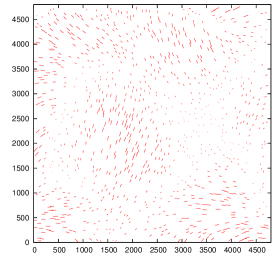
Figure 16: PSF pattern of a starfield from the GREAT10 challenge. The $x$- and $y$-axis are pixel units.

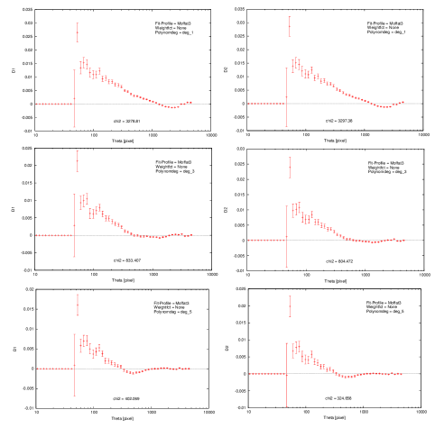
Figure 17: The diagnostic functions $D_{1}$ (left column) and $D_{2}$ (right column) as function of pixel units. The three rows from top to bottom show the case of a PSF interpolation model as bi-variate polynomial in $x$ and $y$ of order 1, 3, and 5, respectively. Figure from Bernhard Riedl’s master thesis (unpublished).

4.4.2 CFHTLenS

The CFHTlenS collaboration created image simulations (1) to calibrate for shear biases (Sect. 4.1.1), and (2) to model residual systematics correlations (Sect. 4.3).

As a cross-check, two sets of simulations were created, using the (modified) code from the GREAT08 and GREAT10 challenges as described in 2010MNRAS.405.2044B, and the SkyMaker package (2009MmSAI..80..422B *2009MmSAI..80..422B), respectively. Several important features were added to the simulations compared to the GREAT challenge:

First, the galaxies were modeled as disk+bulge as fitted by lensfit, with ellipticity and size distribution matching the observed data. A mismatch would result in a wrong bias calibration; for example, the STEP and GREAT08/10 simulations did not include the large observed number of small galaxies, and thus the bias of those objects could not be calibrated correctly.

The additive and multiplicative biases were fitted to all simulated galaxies as functions of size and SNR. I propagated the uncertainties of $m$ from the fits to the correlation function covariance. Their contribution turned out to be negligeable, see Fig. 18.

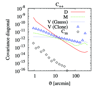
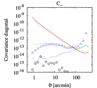
Figure 18: Diagonal of the covariances $\bm{\mathrm{C}}_{++}$ (left panel) and $\bm{\mathrm{C}}_{--}$ (right panel). The variance $\bm{\mathrm{C}}_{m}$ due to the shear calibration of $m$ (black diamonds) is sub-dominant compared to the shot noise $\bm{\mathrm{D}}$ (solid red line), mixed term $\bm{\mathrm{M}}$ (green dashes), and cosmic variance $\bm{\mathrm{V}}$ (blue dashes: Gaussian approximation; blue triangles: non-Gaussian covariance estimated from the CFHTLenS Clone simulations). From CFHTLenS-2pt-notomo.

Second, each galaxy got assigned a shear from the CFHTLenS “Clone” $N$-body simulation (CFHTLenS-Clone *CFHTLenS-Clone). A realistic cosmological shear component is important in the quantitative analysis of systematics (CFHTLenS-sys *CFHTLenS-sys).

4.4.3 GREAT3

The GREAT3 weak-lensing image challenge [2013arXiv1308.4982M] was organised by R. Mandelbaum and B. Rowe, and ran from mid-2013 to April 2014. Results were presented and discussed at the final meeting at CMU in Pittsburgh in May 2014 [great3-I]. I was part of the “CEA–EPFL” team including from CEA Florent Sureau, Jean-Luc Starck, Fred Maurice Ngolé Mboula, Stéphane Paulin-Henriksson, and from EPFL Marc Gentile and Frédéric Courbin.

I also submitted results under “CEA_denoise”, for which I first denoised the galaxy images by applying the mr_filter multi-scale wavelet filter to the images [2006A&A...451.1139S]. I then used SExtractor [1996A&AS..117..393B] to measure unweighted second moments of the galaxy light distribution, and corrected for the PSF in moment space, following 2000ApJ…536…79R, as mentioned earlier. The results were however not great and could not compete with the leading group of best methods.

The main shape measurement method of our team was the forward-fitting maximum-likelihood method gfit. This algorithm is a new version (rewritten in python from scratch) of gfit presented in 2012arXiv1211.4847G, which was used in the GREAT10 galaxy challenge. Galaxies are detected by a SExtractor run, whose output parameters of centroid position, size, and ellipticity are used as first-guess starting point of the model fitting procedure. Galaxy light profiles are modeled as bulge (Sérsic index $n=1$ + exponential (Sérsic $n=4$) disk, which are concentric and aligned with identical intrinsic ellipticity. The eight parameters centroid, flux, disc flux fraction, bulge radius, disk radius, and ellipticity were fitted. Several minimizers were explored.

Weighing and filtering

Often, measured galaxy shapes are weighted depending on various quantities: the galaxy S/R, size, or the best-fit $\chi^{2}$, fit error bar, or confidence in the result. This down-weighs galaxies with uncertain or biased shape estimates and generally improves the results.

Each of the GREAT3 images had $10,000$ galaxies, where two pairwise galaxies had the same intrinsic ellipticity roated by $90\deg$ to reduce shape noise. To fully benefit from this noise cancelling scheme, one has an interest to weigh all galaxies equally. However, for some objects no shape can be attributed, for example if the minimizer does not converge. Thus, at the end of the day, we decided to introduce weights for the galaxies with the hope to reduce the biases.

A first, simple weighing scheme was to eliminiate galaxies with large fit residuals by setting their weight to zero. I then developed an improved weighting scheme, which I describe in the following.

For a given GREAT3 image, the gfit output parameters for each galaxies were used to create new simulations of that image, with properties of noise, PSF, pixellation etc. similar to the input image. gfit was run on this second simulated image, and a PCA decomposition of measured galaxy parameters was performed on the rms ellipticity between input and ouput, $|\Delta e|$. In other words, the galaxies were classified according to ellipticity bias. Using PCA I could identify combinations $v_{i}$ of galaxy parameters that contribute most to this bias, and to devise a weighting scheme to downweigh objects for which those parameters correlated with a large bias. To keep the number of parameters reasonably small, I split them up into several sets of parameters, and studied one set at a time. Here, I will quote results from one such set of parameters (case ‘a’ in [great3-I]), which are the gfit flux $\ln(\ln I_{0})$, disc radius $\ln r_{\rm disk}$, bulge radius $\ln r_{\rm bulge}$, disc flux fraction $f_{\rm disk}$.

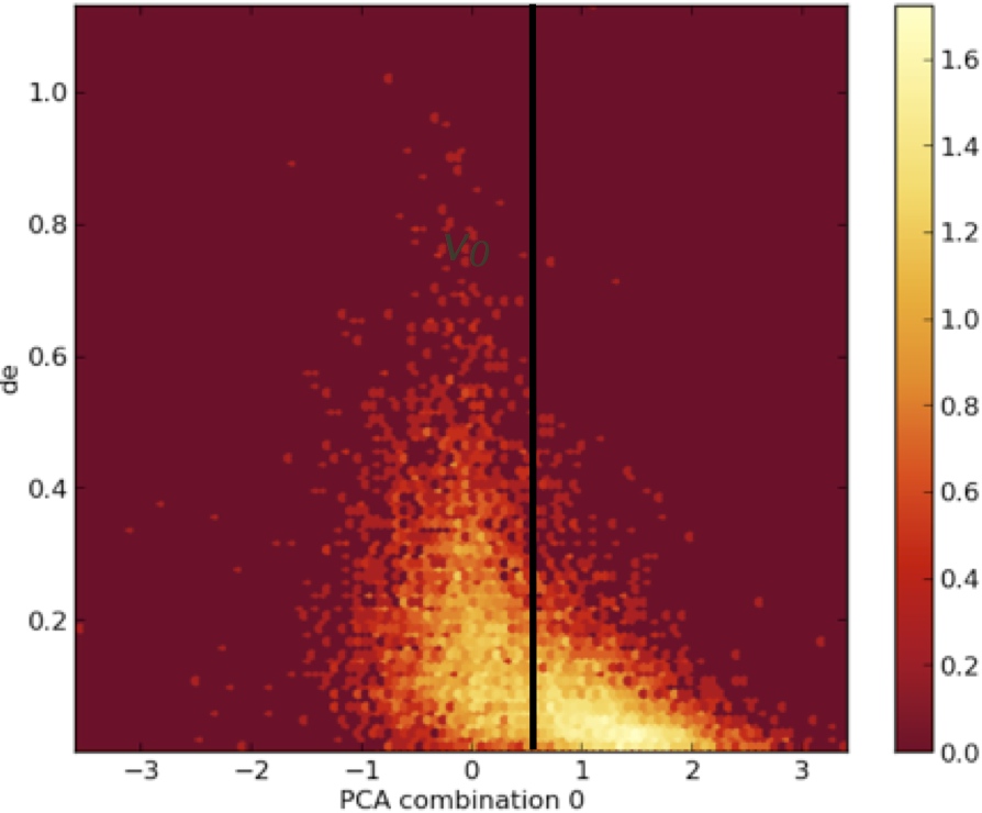
Figure 19: Log-density of objects as function of PCA component $v_{0}$ ($x$-axis) and ellipticity bias $|\Delta e|$ ($y$-axis). The horizontal line is the cut-off value $v_{\rm c}=0.6$.

.

The dependence of the parameters (linear, logarithmic or double-logarithmic) being most significant to quantify large residuals was established by trying out various variants.

The weights were determined by ploting $|\Delta e|$ versus various PCA components $v_{i}$ to select a cutoff value $v_{\rm c}$ that provided a good separation of objects with low and high bias $|\Delta e|$.

A density plot in $v_{0}$ (the $0^{\rm th}$ PCA component) and the ellipticity bias $|\Delta e|$ is show in Fig. 19. There is a clear tail of high-$|\Delta e|$ objects for small values of $v_{0}$, whereas there is a high density of objects with low $|\Delta e|$ at $v_{0}=1\ldots 2$. The cut-off value $v_{\rm c}=0.6$ is shown by the horizontal line. Thus, objects with PCA component $v_{0}<v_{\rm c}$ ($v_{0}>v_{\rm c}$) show generally a strong (weak) bias $|\Delta e|$. The first category was assigned the weight $w_{\rm low}=0.2$. Objects in the low-bias category kept their weight $w_{\rm high}=1$.

The $0^{\rm th}$ PCA component is

$$v_{0} =0.38\ln(\ln I_{0})+0.59r_{\rm disk}+0.44\ln r_{\rm bulge}-0.28f_{\rm disk}$$ (74)

$$=\ln\left[(\ln I_{0})^{0.38}\,r_{\rm disk}^{0.59}\,r_{\rm bulge}^{0.44}\,{\rm e}^{-0.28f_{\rm disk}}\right].$$

This means that the bias is smaller for objects with larger flux, disk and bulge radius, but smaller disk fraction. The improvement on the overall GREAT3 of this weighting scheme compared to uniform weights was around $15$ - $20\%$.

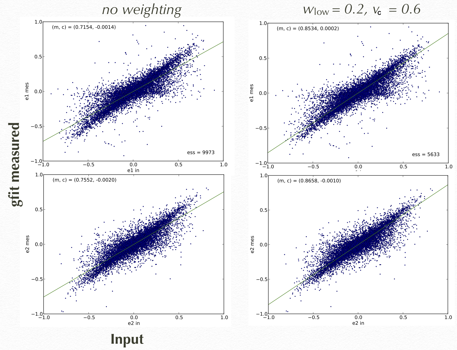
Figure 20: Input ($x$-axes) versus output ($y$-axes) ellipticity ellipticity bias. The upper row is $e_{1}$, the lower row $e_{2}$. Left panels show the no-weighting (uniform weighting) case, the left column is for case (a) with a weight $w_{\rm low}=0.2$ of high-bias objects whose $0^{\rm th}$ PCA component is smaller than $v_{\rm c}=0.6$. The lines are fits of multiplicative ($m$) and additive ($c$) bias with values indicated in the panels.

.

4.5 Redshift estimation

4.5.1 Photometric redshifts

Weak lensing observables, being integrals along the line of sight weighted by the source galaxy distribution $n(z)$ (23), require knowledge of the latter if they are to be interpreted cosmologically. To first order, the mean redshift $\bar{z}$ has to be determined, but also the shape of $n(z)$ plays an important role. 2006MNRAS.366..101H find a rough estimate of $P_{\kappa}(\ell\sim 1000)\propto\Omega_{\rm de}^{-3.5}\sigma_{8}^{2.9}{\bar{z}}^{1.6}|w|^{0.31}$. Clearly, for a desired accuracy on cosmological parameters, the mean redshift of sources has to be known to at least that accuracy, and to a much higher accuracy in the case of parameter on which the power spectrum has a weaker dependence such as $w$.

Spectroscopy of all the faint galaxies used for a typical weak-lensing survey is too costly, and redshifts have to be estimated from broad-band photometry, using the technique of photometric redshifts, or photo-$z$s. There are various methods to measure photometric redshifts, of which template-based approaches are one of the most popular. They perform $\chi^{2}$-type fits of (redshifted) template SEDs to the flux in the observed bands. Exemplary methods that have been used in a weak-lensing context include LePhare [2006A&A...457..841I] and Bayesian Photometric redshift estimation 2000ApJ…536..571BBPZ; . LePhare photo-$z$’s for CFHTLS were published in [CIK09]; BPZ was the method of choice for CFHTLenS [CFHTLenS-photoz]. Both methods do not only performe a point-estimate $\hat{z}$ but provide the full pdf of the redshift.

4.5.2 Clustering-based redshift estimation

To assess the quality of photometric redshifts and to recover the true redshift distribution, one can make use of the spatial clustering of galaxies. From the amount of cross-correlation of photometric samples between different redshift bins one can deduce the amount of redshift outliers. In BvWMK10 we introduced this method, and applied it to photometric clustering [CK11, MWCK15] and weak-lensing [CFHTLenS-2pt-tomo].

Fig. 21 is an example from CK11. For the full galaxy sample of the CFHTLS-Wide T0006 release, it shows the angular auto-correlation functions of redshift bin #1, $0.4<z<0.6$, and the two auto-correlation functions of that bin with galaxies at higher redshift bins #3 ($0.8<z<1$) and #4 ($1<z<1.2$), respectively. From these measurement we estimate the contamination $f_{ij}$ between redhift bin pairs $i$ and $j$ due to photometric mis-identification. We carry out the so-called global pair-wide analysis, considering only two bins at a time while in turn setting to zero contaminations of other bins, and also neglecting higher-order effects such as magnification bias. The resulting constraints of the contamination fractions, $f_{ij}$, $i,j=1,3,4$, are shown in the in the middle and right panels. Around three percent of galaxies in bin #3 are mis-identified into bin #1, which leads to the non-zero cross-correlation between the two bins (dotted line in the left panel). The mixing between bins #1 and #4 is consistent with zero, as is the cross-correlation function (dashed line in the left panel).

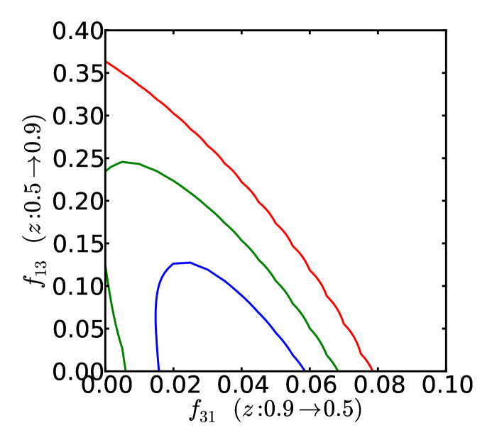
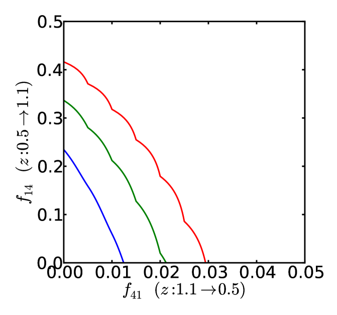
Figure 21: Cross correlation analysis between redshift bins for the full sample. Left: angular auto-correlation function in the redshift bin $0.4<z<0.6$ (straight line) and cross-correlation between the bins $0.4<z<0.6$ and $0.8<z<1.0$ (dotted line) and between $0.4<z<0.6$ and $1.0<z<1.2$ (dashed line). Middle and right: quantitative estimates of the contamination (percentage of galaxies scattered) from a pairwise analysis between redshift bins $0.4<z<0.6$ and $0.8<z<1.0$ (middle) and between $0.4<z<0.6$ and $1.0<z<1.2$ (right). The contours show the 68.3 (blue), 95.5 (green) and 99.7 (red) confidence regions. From CK11.

Similarly, the cross-correlation of the photometric with a spectroscopic sample can reveal the true redshift distribution [Newman08], although this reconstruction is hampered by a possible redshift-dependent bias of the photometric galaxy sample [2010ApJ...724.1305S]. In Scottez16 we applied the cross-correlation method to CFHTLS/VIPERS, and showed that it can yield redshifts for individual galaxies if color information is present.

5 Observational results and cosmological constraints

This section highlights some of the observational results for cosmological parameter constraints from cosmic shear to which I contributed.

5.1 Second-order statistics

In the following sub-sections I discuss the basic observational results from second-order cosmic shear statistics. The parameter combination that cosmic shear (including non-linear scales) is most sensitive to the parameter $\Sigma_{8}$, defined by

$$\Sigma_{8}=\sigma_{8}\left(\frac{\Omega_{\rm m}}{\Omega_{\rm m,0}}\right)^{\alpha},$$ (75)

with typical values of $\alpha\approx 0.5$ - $0.7$. The pivot value $\Omega_{{\rm m},0}$ can be chosen freely. Fig. 22 and Table LABEL:tab:Sigma shows this combination measured in recent years for $\Omega_{\rm m,0}=0.3$. If the original measurement (indicated in the table) corresponds to a different pivot value, I transform to $\Omega_{\rm m,0}=0.3$ including a simple error propagagtion computation.

5.1.1 CFHTLS-T0003, 2007

The third data release (T0003) of the wide part of the Canada-France-Hawaii Telescope Legacy Survey (CFHTLS) with an observed area of $53$ deg² provided 2D cosmic shear results out to very large, linear scales FSHK08$7.7$ degrees, corresponding to $170$ Mpc at the mean lens redshift of $0.5$; . This enabled us to infer cosmological constraints using large scales only, thereby reducing uncertainties from non-linear and baryonic physics on small scales. Using $\langle M_{\rm ap}^{2}\rangle(\theta)$ on scales $\theta>85^{\prime}$ we obtained $\sigma_{8}(\Omega_{\rm m}/0.25)^{0.53}=0.837\pm 0.084$. This study used the photometric redshifts from the 4 square degree deep part of CFHTLS [2006A&A...457..841I], taking into account sampling variance. The deep fields have an area of $4$ square degrees, an increase of nearly a factor $2500$ over the HDF. Constraints on neutrino masses were obtained using this data release in TSUK09.

By that time, ground-based surveys had become large enough to enable detailed residual systematics tests. For CFHTLS, KB09 as well as first multi-colour observations [FuPhD] revealed an anomalous shear amplitude scaling with source redshift and a variance between MegaCam pointings larger than expected. KB09 quantified their influence on cosmological parameters from a joint analysis. However, it took three more years of work by the CFHTLenS team (Sect. 5.1.3) of around 20 members and a complete re-analysis of CFHTLS images to finally obtain a robust shear catalogue. The origin of those systematics was never found, and the price to pay for a systematic-free data set was to reject $25\%$ of the MegaCam pointings that were plagued with PSF residuals.

5.1.2 Re-analysis of COSMOS, 2009

I contributed to a re-analysis of the weak-lensing data [SHJKS09], independent from the first series of papers from that survey [2007ApJS..172..219L, 2007ApJS..172..239M]. We obtained improved photo-$z$’s from twice the number of bands [2009ApJ...690.1236I]. Due to the low number of high-$S/N$ stars in ACS fields, and temporal instabilities of HST, the PSF model was obtained by PCA of the PSF pattern from dense stellar fields. In this work we presented a five-bin tomographic analysis, leading to constraints on the deceleration parameter $q_{0}=-\ddot{a}a/\dot{a}^{2}=\Omega_{\rm m}/2-\Omega_{\Lambda}$, with a detection of acceleration ($q_{0}<0$) at 94.3% confidence, including additional priors on $h$ and $\Omega_{\rm b}$.

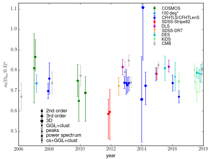
Figure 22: Mean and 68% error bars for the parameter $\sigma_{8}\left(\Omega_{\rm m}/0.3\right)^{\alpha}$, for various cosmic shear observations, plotted as function of their publication date (first arXiv submission). All parameter values are given in Table LABEL:tab:Sigma. Different surveys are distinguished by colour as indicated in the figure. Data points are shown for second-order statistics (circles), third-order (diamonds), 3D lensing (pentagons), galaxy-galaxy lensing (+ galaxy clustering; triangle), and CMB (squares). This plot is an updated version of Fig. 7 from K15.

Table 3: Parameter values of $\sigma_{8}\Omega_{\rm m}^{\alpha}$ used for Fig. 22. For different surveys (first column) the second column is the value rescaled to $\Omega_{\rm m}=0.3$ which is plotted in the figure, obtained from the original measurement (third column). The fourth column indicates the number of redshift bins, the column 5 is the reference. This table is an updated version of Table 1 from Kilbinger (2015). ^a 5 narrow photo-$z$ bins and one wide bin of faint galaxies. ^b 3D lensing, no $z$-binning. ^c The index $\alpha=0.5$ is adopted from the WMAP9 measurement, published on http://lambda.gsfc.nasa.gov. The resulting values and errors are therefore only illustrative.

Survey	$\sigma_{8}(\Omega_{\rm{m}}/0.3)^{\alpha}$	originalxmeasurement		$N_{z}$	Reference
COSMOS	$0.810\pm{0.17}$	$\sigma_{8}(\Omega_{\rm{m}}/0.3)^{0.48}$ =	$0.81\pm{0.17}$	1	2007ApJS..172..239M
COSMOS	$0.866^{+0.085}_{-0.068}$	$\sigma_{8}(\Omega_{\rm{m}}/0.3)^{0.44}$ =	$0.866^{+0.085}_{-0.068}$	3	2007ApJS..172..239M
100xdeg2	$0.736\pm{0.0438}$	$\sigma_{8}(\Omega_{\rm{m}}/0.24)^{0.59}$ =	$0.84\pm{0.05}$	1	JonBen07
CFHTLS	$0.699\pm{0.0383}$	$\sigma_{8}(\Omega_{\rm{m}}/0.25)^{0.64}$ =	$0.785\pm{0.043}$	1	FSHK08
CFHTLS	$0.760\pm{0.0763}$	$\sigma_{8}(\Omega_{\rm{m}}/0.25)^{0.53}$ =	$0.837\pm{0.084}$	1	FSHK08,xlargexscales
COSMOS	$0.750\pm{0.08}$	$\sigma_{8}(\Omega_{\rm{m}}/0.3)^{0.51}$ =	$0.75\pm{0.08}$	$5\!+\!1^{a}$	SHJKS09
COSMOS	$0.650\pm{0.1}$	$\sigma_{8}(\Omega_{\rm{m}}/0.3)^{0.62}$ =	$0.65\pm{0.1}$	1	SHJKS09
COSMOS	$0.69^{+0.08}_{-0.14}$	$\sigma_{8}(\Omega_{\rm{m}}/0.3)^{0.46}$ =	$0.69^{+0.08}_{-0.14}$	1	2011MNRAS.410..143S,x$+$IA
SDSS-Stripe82	$0.585^{+0.0743}_{-0.121}$	$\sigma_{8}(\Omega_{\rm{m}}/1.0)^{0.7}$ =	$0.252^{+0.032}_{-0.052}$	1	2012ApJ…761…15L
SDSS-Stripe82	$0.597^{+0.11}_{-0.138}$	$\sigma_{8}(\Omega_{\rm{m}}/0.264)^{0.67}$ =	$0.65^{+0.12}_{-0.15}$	1	2011arXiv1112.3143H
SDSS-DR7	$0.721\pm{0.0451}$	$\sigma_{8}(\Omega_{\rm{m}}/0.25)^{0.57}$ =	$0.8\pm{0.05}$	1	2013MNRAS.432.1544M
DLS	$0.816\pm{0.0385}$	$\sigma_{8}(\Omega_{\rm{m}}/0.265)^{0.5}$ =	$0.868\pm{0.041}$	1	2012arXiv1210.2732J,xpriv. comm.
CFHTLenS	$0.740\pm{0.0301}$	$\sigma_{8}(\Omega_{\rm{m}}/0.27)^{0.59}$ =	$0.787\pm{0.032}$	1	CFHTLenS-2pt-notomo
CFHTLenS	$0.738^{+0.0654}_{-0.056}$	$\sigma_{8}(\Omega_{\rm{m}}/0.27)^{0.65}$ =	$0.79^{+0.07}_{-0.06}$	1	CFHTLenS-2pt-notomo,xlargexscales
CFHTLenS	$0.728\pm{0.0377}$	$\sigma_{8}(\Omega_{\rm{m}}/0.27)^{0.55}$ =	$0.771\pm{0.04}$	2	CFHTLenS-2pt-tomo
CFHTLenS	$0.737^{+0.0305}_{-0.0391}$	$\sigma_{8}(\Omega_{\rm{m}}/0.27)^{0.46}$ =	$0.774^{+0.032}_{-0.041}$	6	CFHTLenS-IA,x$+$IA
CFHTLenS	$0.657\pm{0.21}$	$\sigma_{8}(\Omega_{\rm{m}}/0.27)^{0.46}$ =	$0.69\pm{0.22}$	$\infty^{b}$	CFHTLenS-3d,x$+$bary
CFHTLenS	$1.107\pm{0.258}$	$\sigma_{8}(\Omega_{\rm{m}}/0.27)^{0.44}$ =	$1.16\pm{0.27}$	$\infty^{b}$	CFHTLenS-3d,xlargexscales,$+$bary
CFHTLenS	$0.725^{+0.0659}_{-0.0942}$	$\sigma_{8}(\Omega_{\rm{m}}/0.27)^{0.57}$ =	$0.77^{+0.07}_{-0.1}$	1	CFHTLenS-2+3pt,x$+$IA
CFHTLenS	$0.785^{+0.028}_{-0.0374}$	$\sigma_{8}(\Omega_{\rm{m}}/0.27)^{0.64}$ =	$0.84^{+0.03}_{-0.04}$	1	2014arXiv1412.0757L
SDSS-Stripe82	$0.785\pm{0.0287}$	$\sigma_{8}(\Omega_{\rm{m}}/0.27)^{0.42}$ =	$0.82\pm{0.03}$	1	2014arXiv1412.3683L
DES-SV	$0.811^{+0.059}_{-0.06}$	$\sigma_{8}(\Omega_{\rm{m}}/0.3)^{0.478}$ =	$0.811^{+0.059}_{-0.06}$	3	2015arXiv150705552T
DLS	$0.818^{+0.034}_{-0.026}$	$\sigma_{8}(\Omega_{\rm{m}}/0.3)^{0.5}$ =	$0.818^{+0.034}_{-0.026}$	5	2015arXiv151003962J
CFHTLenS	$0.738\pm{0.0393}$	$\sigma_{8}(\Omega_{\rm{m}}/1.0)^{0.5}$ =	$0.404\pm{0.0215}$	7	2016arXiv160105786J,x$+$IA,bary,$z$-sys
DES-SV	$0.770\pm{0.07}$	$\sigma_{8}(\Omega_{\rm{m}}/0.3)^{0.6}$ =	$0.77\pm{0.07}$	1	2016arXiv160305040K
CFHTLenS	$0.670\pm{0.03}$	$\sigma_{8}(\Omega_{\rm{m}}/0.3)^{0.5}$ =	$0.67\pm{0.03}$	2	2016arXiv160700008A,x$z$-sys
KiDS	$0.745\pm{0.039}$	$\sigma_{8}(\Omega_{\rm{m}}/0.3)^{0.5}$ =	$0.745\pm{0.039}$	4	KiDS-450,x$+$IA,bary,$\Delta{n(z)}$
KiDS	$0.801\pm{0.032}$	$\sigma_{8}(\Omega_{\rm{m}}/0.3)^{0.5}$ =	$0.801\pm{0.032}$	4	2017arXiv170605004V,xcs+ggl+clust,band-power,$+$IA,bary,$\Delta{n(z)}$
KiDS	$0.742\pm{0.035}$	$\sigma_{8}(\Omega_{\rm{m}}/0.3)^{0.5}$ =	$0.742\pm{0.035}$	4	2017arXiv170706627J,xcs+ggl+RSD,$+$I-A,bary,$\Delta{n(z)}$
KiDS	$0.696^{+0.048}_{-0.05}$	$\sigma_{8}(\Omega_{\rm{m}}/0.3)^{0.38}$ =	$0.696^{+0.048}_{-0.05}$	1	2018MNRAS.474.1116S,xhigh-SNR-peaks
DES-Y1	$0.789^{+0.024}_{-0.026}$	$\sigma_{8}(\Omega_{\rm{m}}/0.3)^{0.5}$ =	$0.789^{+0.024}_{-0.026}$	4	2017arXiv170801538T
DES-Y1	$0.783^{+0.021}_{-0.025}$	$\sigma_{8}(\Omega_{\rm{m}}/0.3)^{0.5}$ =	$0.783^{+0.021}_{-0.025}$	4	2017arXiv170801530D
KiDS	$0.750\pm{0.059}$	$\sigma_{8}(\Omega_{\rm{m}}/0.3)^{0.5}$ =	$0.75\pm{0.059}$	1	2018MNRAS.474..712M,xlow-SNR-peaks
DES-Y1	$0.78^{+0.05}_{-0.04}$	$\sigma_{8}(\Omega_{\rm{m}}/0.3)^{0.5}$ =	$0.78^{+0.05}_{-0.04}$	4-5	2017arXiv171005045G,xdensity-split-statistic
WMAP3c	$0.671\pm{0.0669}$	$\sigma_{8}(\Omega_{\rm{m}}/0.234)^{0.5}$ =	$0.76\pm{0.05}$	-	2007ApJS..170..377S
WMAP5c	$0.738\pm{0.0544}$	$\sigma_{8}(\Omega_{\rm{m}}/0.258)^{0.5}$ =	$0.796\pm{0.036}$	-	WMAP5-Komatsu08
WMAP7c	$0.774^{+0.0512}_{-0.0518}$	$\sigma_{8}(\Omega_{\rm{m}}/0.273)^{0.5}$ =	$0.811^{+0.03}_{-0.031}$	-	2010arXiv1001.4538K
WMAP9	$0.792\pm{0.0529}$	$\sigma_{8}(\Omega_{\rm{m}}/1.0)^{0.5}$ =	$0.434\pm{0.029}$	-	2012arXiv1212.5226H
Planck2013	$0.848\pm{0.0286}$	$\sigma_{8}(\Omega_{\rm{m}}/0.27)^{0.46}$ =	$0.89\pm{0.03}$	-	2013arXiv1303.5076P,x$C(\ell)$
Planck2013	$0.740\pm{0.0242}$	$\sigma_{8}(\Omega_{\rm{m}}/0.27)^{0.3}$ =	$0.764\pm{0.025}$	-	2013arXiv1303.5080P,xSZ
Planck2015	$0.825\pm{0.0161}$	$\sigma_{8}(\Omega_{\rm{m}}/1.0)^{0.5}$ =	$0.4521\pm{0.0088}$	-	2015arXiv150201589P,x$C(\ell)$
Planck2015+SPT	$0.808\pm{0.0324}$	$\sigma_{8}(\Omega_{\rm{m}}/1.0)^{0.25}$ =	$0.598\pm{0.024}$	-	2017arXiv171207541S

5.1.3 CFHTLenS, 2012 - 2015

A milestone for cosmic shear represented the CFHT lensing survey CFHTLenS-dataCFHTLenS; . With CFHTLenS we provided measurements that relied on independently cross-checked photometric redshifts, and a robust estimate of residual systematics on weak-lensing shear correlations (Sect. 4.3). In these studies, the residual sytematics analysis was done completely independently from the cosmological parameters analysis, in order not to bias the cosmological results.

Flat $\Lambda$CDM

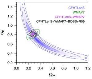
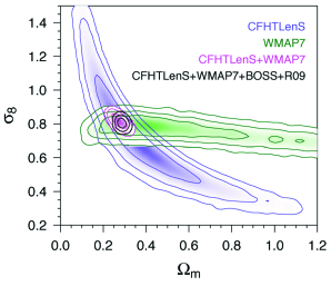
Figure 23: The 2D cosmic shear and CMB. CFHTLenS, WMAP7, BAO from BOSS [2012arXiv1203.6594A], and a HST $H_{0}$ prior [2009ApJ...699..539R, ‘R09’]. From CFHTLenS-2pt-notomo.

Photometric redshifts for each source galaxy were obtained in CFHTLenS-photoz, the robustness of which was verified using spectroscopic redshifts, COSMOS 30-band photo-$z$s, and a cross-correlation analysis [CFHTLenS-2pt-tomo]. Galaxy shapes were measured on individual exposures with lensfit and calibrated using two independent suites of image simulations [CFHTLenS-shapes]. An excess correlation between star and galaxy shapes (69) was found on $25\%$ of the observed fields, which in turn were discarded from the cosmological analysis [CFHTLenS-sys]. Two-dimensional cosmic shear correlation functions from CFHTLenS were presented in CFHTLenS-2pt-notomo. A two-bin tomographic analysis was performed by CFHTLenS-2pt-tomo. The same tomographic data were used to place constraints on modified gravity [CFHTLenS-mod-grav]. Further, a six-bin tomographic analysis was performed where cosmological and intrinsic-alignment parameters were constrained simultaneously [CFHTLenS-IA]. Late-type galaxies were found to not show any significant intrinsic alignment, while for early type galaxies IA was detected at about $2\sigma$.

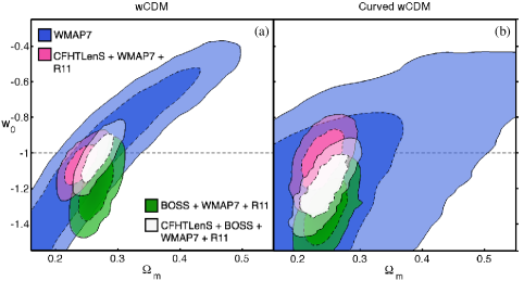
Figure 24: Combined constraints on $\Omega_{\rm m}$ and $w_{0}$ from cosmic shear, CMB, and BAO. The model is a $w$CDM universe with flat (free) curvature in panel a (b). Cosmic shear is six-bin tomography from CFHTLenS. The CMB and BAO data are the same as in Fig. 23. The HST $H_{0}$ prior is replaced with an updated version [2011ApJ...730..119R]. From CFHTLenS-IA.

For a $\Lambda$CDM cosmology, cosmic shear constrains a combination of $\Omega_{\rm m}$ and $\sigma_{8}$ that is perpendicular to the one obtained from CMB [Contaldi03]. Adding cosmic shear to WMAP (Wilkinson Microwave Anisotropy Probe) results in typical reduction of error bars on $\Omega_{\rm m}$ and $\sigma_{8}$ of up to $50\%$, similar to other low-$z$ cosmological probes such as Baryonic Acoustic Oscillations (BAO). For example, the WMAP7 constraints of $\Omega_{\rm m}=0.273\pm 0.03$ and $\sigma_{8}=0.811\pm 0.031$ [2010arXiv1001.4538K] get tightened when adding CFHTLenS, resulting in $\Omega_{\rm m}=0.274\pm 0.013$ and $\sigma_{8}=0.815\pm 0.016$ [CFHTLenS-2pt-notomo], see Fig. 23. Planck’s cosmological findings from temperature anisotropies (together with CMB lensing and WMAP polarization) correspond to a higher matter density and normalization compared to most previous pobes, with $\Omega_{\rm m}=0.315\pm 0.017$ and $\sigma_{8}=0.829\pm 0.012$, or $\sigma_{8}(\Omega_{\rm m}/0.27)^{0.46}=0.89\pm 0.03$ [2013arXiv1303.5076P]. This is consistent with CFHTLenS at the $2\sigma$ level, see Fig. 25. Further, Planck’s counts of Sunyaev-Zel’dovich (SZ) clusters results in a lower normalization of $\sigma_{8}(\Omega_{\rm m}/0.27)^{0.3}=0.78\pm 0.01$ [2013arXiv1303.5080P]. Sect. 5.1.4 discusses whether adding extra-parameters such as massive neutrinos are needed to reconcile recent high- and low-$z$ data.

A model with variable curvature does not change the cosmic-shear constraints on $\Omega_{\rm m}$ and $\sigma_{8}$ by a lot. Pre-Planck CMB data alone cannot constrain the curvature of the Universe, and adding other probes such as measurements of $H_{0}$ or weak lensing are required. Planck and high-resolution ground-based millimetre-wavelength radio telescopes of similar sensitivity and resolution such as SPT (South Pole Telescope) and ACT (Atacama Cosmology Telescope) have detected weak-lensing of the CMB by large-scale structures (CMB lensing), which helps to break the geometrical degeneracy. This results in tight constraints on $\Omega_{K}$ from CMB alone [2011PhRvL.107b1302S, 2012ApJ...756..142V, 2013arXiv1303.5076P]. Fig. 25 shows joint cosmic shear and CMB constraints for a free-curvature model.

Since the effect of dark energy on the supression of the growth of structure is relatively small, 2D weak lensing is not very sensitive to dark energy. Tomographic weak lensing can place interesting constraints on the dark-energy equation of state parameter. Fig. 24 shows how CMB constraints from WMAP7 — with an additional prior on $H_{0}$ from 2011ApJ…730..119R — are reduced by CFHTLenS six-bin tomography. The parameters $\Omega_{\rm m}$ and $w_{0}$ are measured to better than $10\%$ accuracy, for both a flat and free-curvature $w$CDM model. The improvement is similar to adding Baryonic Acoustic Oscillation (BAO) data from the SDSS-III Baryon Oscillation Spectroscopic Survey 2012arXiv1203.6594ABOSS; to CMB data.

Constraints on modified gravity using the parametrization in eqs. (6, 7) showed consistency with GR [CFHTLenS-mod-grav]. A simple model was considered where $\Sigma$ and $\mu$ did not vary spatially, and at early times tend towards GR, so that deviations of GR are allowed at late times where the accelerated expansion happens. The present-day values of those two parameters were measured to be $\Sigma_{0}=0.00\pm 0.14$, and $\mu_{0}=0.05\pm 0.25$, combining CFHTLenS weak-lensing tomographic data [CFHTLenS-2pt-tomo], redshift-space distortions from WiggleZ [2012MNRAS.425..405B] and 6dFGS [2012MNRAS.423.3430B], WMAP7 CMB anisotropies from small scales, $\ell\geq 100$ [2011ApJS..192...16L], and the 2011ApJ…730..119R $H_{0}$ prior (see Fig. 26).

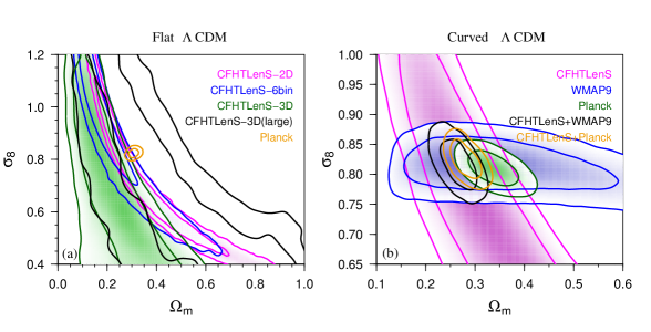
Figure 25: Cosmic shear and CMB $68.3\%$ and $95.5\%$ confidence levels for $\Omega_{\rm m}$ and $\sigma_{8}$ in a $\Lambda$CDM universe. (a) Assuming flatness. CFHTLenS 2D, 6-bin tomography, 3D, and 3D from large scales only are compared to Planck constraints. (b) With free curvature, showing CFHTLenS (joint second- and third-order), WMAP9, Planck, CFHTLenS $+$ WMAP9, and CFHTLenS $+$ Planck constraints, from CFHTLenS-2+3pt.

5.1.4 Further results from CFHTLenS

Other groups different from the CFHTLenS collaboration have used those data for further, extended analysis. The cosmological constraints from CMB temperature anisotropies measured by the Planck satellite [2013arXiv1303.5076P] seem to be in slight tension with other probes. In particular, Planck found a higher power-spectrum normalisation $\sigma_{8}$. Several works proposed massive neutrinos to alleviate the tension with low-$z$ probes such as weak lensing: Massive neutrinos are still relativistic at recombination and do not significantly influence the CMB anisotropies. They become however non-relativistic at late time, and dampen the growth of structure, therefore reducing the low-$z$ clustering power. Joint analyses including massive neutrinos from Planck and our CFHTLenS weak-lensing data of CFHTLenS-2pt-notomo were found to improve parameter constraints with the inclusion of non-zero neutrino masses [2014PhRvL.112e1303B, 2014arXiv1403.4599B], but the evidence still favors a $\Lambda$CDM model without additional parameters for massive neutrinos [2014arXiv1404.5950L].

Flat $\Lambda$CDM

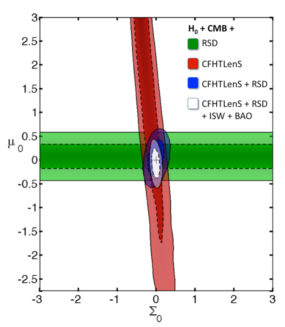
Figure 26: Combined constraints on the present-day modified-gravity parameters $\Sigma_{0}$ and $\mu_{0}$, from redshift-space distortions (RSD), cosmic shear (CFHTLenS), and their combination, including the case of additional BAO [2012arXiv1203.6594A] and large-scale WMAP7 (ISW) data. All data are combined with a $H_{0}$ prior and small-scale CMB data, see text. From CFHTLenS-mod-grav.

5.2 Higher-order correlations

The motivation behind higher-order shear statistics has been argued for in Sect. 2.3. Even though the measurement is challenging and the overall signal-to-noise ratio is low, several significant detections of third-order shear correlations have been made.

Several higher-order measurements resulted from CFHTLenS. First, CFHTLenS-kappa-maps measured the skewness of reconstructed convergence maps and found good agreement with WMAP7 predictions. After validating the data for shear residual third-order correlations, CFHTLenS-3pt performed a cosmological analysis of the aperture-mass skewness exploring a non-Gaussian likelihood. CFHTLenS-2+3pt combined the second- and third-order aperture-mass combined with WMAP9 and Planck to obtain cosmological results (see Fig. 25), including models of intrinsic alignment and source-lens clustering as astrophysical systematics.

Quite a few measurements of weak-lensing peak counts were obtained using data from the CFHT/MegaCam Stripe-82 survey (CS82), CFHTLenS, the Dark Energy Survey (DES), and the Kilo-Degree Survey (KiDS) [2013arXiv1311.1319S, 2014arXiv1412.0757L, 2014arXiv1412.3683L, 2016arXiv160305040K, 2018MNRAS.474..712M]. Preliminary measurements on the combination of DES (SVD; science verification data), KiDS data release DR1/2, and CFHTLenS, and comparison to our fast stochastic models are presented and discussed in Chieh-An Lin’s PhD thesis [2016arXiv161204041L].

5.3 Intrinsic alignment

In FSHK08 we tried to obtain constraints on intrinsic alignment. Since we had no redshift information and therefore one large redshift bin, the different contributions to the shape correlation function of cosmic shear ($GG$) and shear-shape intrinsic alignment ($GI$) are not easily separated. The shape-shape alignment ($II$) cannot be resolved with a wide redshift distribution. We therefore obtained a non-detection of $GI$, with $A=2.2^{+3.8}_{-4.6}\times 10^{-7}h/{\rm Mpc}$, using the simple model of Heymans06. No evidence pointed to the presence of $GI$ above the statistical and systematic error level.

A $2\sigma$ detection of intrinsic alignment from early-type galaxies was obtained by jointly fitting cosmology and the 2004MNRAS.353..529H linear IA model to CFHTLenS cosmic shear tomographic data [CFHTLenS-IA]. Fig. 27 shows a systematic lower amplitude of shear correlation for cross-redshift correlations compared to the cosmic-shear prediction, as expected from a negative $GI$ contribution. No detection was found for the late-type sample.

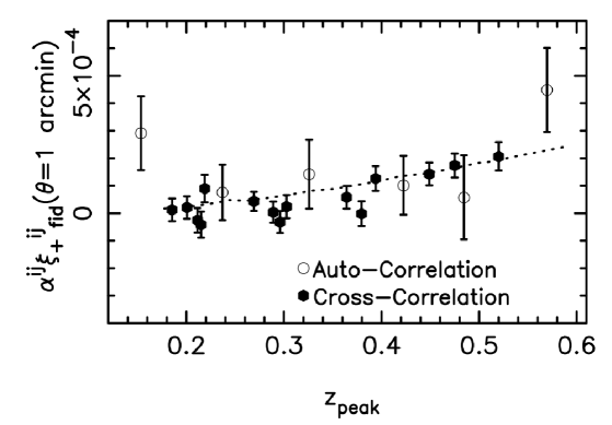
Figure 27: Amplitudes of tomographic measures of $\xi_{+}$ at $\theta=1$ arcmin for redshift bins $(ij)$, against peak lensing efficiency redshift $z_{\rm peak}$ for early-type galaxies, from CFHTLenS. The free parameters $\alpha^{ij}$ multiplied with a WMAP7 fiducial $GG$ model $\xi_{+\rm fid}$ were fitted to $\xi_{+}$ and $\xi_{-}$, simultaneous for all redshift bins and angular scales. At low $z$, the auto-correlations ($i=j$, open circles) lie above the fiducial dashed line ($a^{ij}=1$), as expected for a $II>0$ contribution. The cross-correlations ($i\neq j$, filled circles) lie systematically below the prediction, indicating a $GI<0$ contamination. From CFHTLenS-IA.

6 Future cosmic shear expectations and forecasts

6.1 Upcoming and future surveys

New instruments, either cameras, telescopes, or both, are being designed and built specifically for the purpose of weak-lensing observations. Their design is driven by the goal to provide superb image quality with very small, uniform, and well-understood image distortions. The pixel scale is chosen to sufficiently sample the PSF. In view of the enormous costs of new experiments, in particular space missions, the instruments have to be thoroughly and carefully designed to guarantee the desired scientific outcome, for example, the measurement of dark-energy properties with a given accuracy.

In early 2017, CFIS, the Canada-France Imaging Survey will start observations. CFIS is attributed around 200 nights over three years, to map the Northern sky in $u$ and $r$. The $u$-band part (CFIS-LUAU) will complement the on-going LUAU program, and cover at the end $10,000$ square degree, with a limiting magnitude of $u=24.4$. The $r$-band survey, CFIS-WIQD (for Wide + Image Quality + Deep) will obverse $4,800$ deg² north of $\delta>30\degree$ and galactic latitude $b>25\degree$, to a depth of $r=24.85$.

Despite only observing in two bands (with a rather shallow $u$ component), CFIS will be very interesting for weak lensing, in particular in combination with deep spectroscopic surveys such as eBOSS and DESI. Such deep data does not exist in the Southern hemisphere. CFIS will also contribute to DESI target selection and provide photometric bands for Euclid photo-$z$’s.

Going to space offers the two major advantages: Escaping atmospheric turbulence leads to a stable and small PSF, and infrared observations provide photo-$z$s to significantly higher redshifts than from the ground.

The accessible extra-galactic sky (the area outside the Milky Way and the ecliptic) of $15,000$ deg² will be observed from space with the ESA satellite mission Euclid [2011arXiv1110.3193L]. The two main science drivers for Euclid are cosmic shear and galaxy clustering, which will be observed using three instruments, an optical imager, a near-infrared imager, and a near-infrared slitless spectrograph. The optical imager on board Euclid is designed to have a very stable PSF, both spatially as well as in the time domain. To collect enough galaxy light from billions of high-redshift galaxies ($30\,\mbox{arcmin}^{-2}$), the transmission curve is very broad, corresponding to the combined $R+I+z$ filters, with a required depth of $R+I+z=24.5$. This poses new challenges to overcome, in particular galaxy colour gradients and PSF calibrations).

Further obstacles unique to space-based observations will have to be tackled [2013MNRAS.431.3103C]: For example, the very small PSF will be undersampled by the pixels of size $0.1$ arcsec. From these undersampled stellar images, a reliable, high-resolution PSF model has to be reconstructed. Furthermore, the detector degrades with time due to the bombardment with cosmic rays, and the shapes of objects get distorted by the so-called charge transfer inefficiency (CTI). Corrections as function of time, position on chip, and brightness of the objects have to be applied [2010MNRAS.401..371M, 2014MNRAS.439..887M].

The shear calibration of the huge data expected from Euclid to the required formidable accuracy will be another challenge. The necessary volume of image simulations for calibration is estimated to be huge, as well as the processing time of those simulations [2016arXiv160903281H]. It is not clear yet whether new, alternative methods such as meta-calibration, can be used: The undersampled galaxy images with very large wavelength range makes devonvolution with the correct PSF challenging, and will require the development of new methods. We are studying sparsity-approaches [2017A&A...601A..66F] that we plan to develop further for Euclid.

6.2 Outlook

In 2000, cosmic shear was first measured over a few square degrees of observed sky, from some ten thousand galaxies. Fifteen years later, surveys have increased these numbers by a factor of $100$, imaging a few million galaxies over ${\cal O}(100)$ square degrees. Many challenges were met to analyse these data, taking years of work. This resulted in constraints on cosmological parameters that are competitive compared to other cosmological probes.

In another ten years, upcoming and future experiments will cover a substantial fraction of the entire sky, measuring billions of galaxies. This signifies yet another data volume increase of a factor of $100$, not to mention the data quality improvement due to instruments dedicated to weak lensing. The formidable challenge here is reducing systematic errors to an acceptable level when analysing these large data sets. New, unprecedented difficulties have to be overcome, for example CTI for Euclid, and blended galaxy images for LSST. To fully exploit those surveys, large follow-up programs are needed to obtain the necessary large samples of photometric and spectroscopic redshifts. In addition, to interpret the results of those surveys, the accuracy of theoretical predictions of the non-linear power spectrum including baryonic physics need to be significantly improved.

If all these challenges can be overcome, weak cosmological lensing has the great potential to advance our understanding of fundamental physics. It can explore the origin of the recent accelerated expansion of the Universe, and distinguish between dark energy models and theories of modified gravity. Cosmic shear can measure initial conditions of the primordial Universe, constrain the mass of neutrinos, and measure properties of dark matter. Not only that, the study of intrinsic galaxy alignments has provided insights into the formation and evolution of high-redshift galaxies in their dark-matter environment, proving that cosmic shear does not only probe cosmology, but influences and enriches other areas of astrophysics. Thus, over the last fifteen years, weak cosmological lensing has established itself as a major tool in understanding our Universe, and with upcoming large surveys, it will continue to be of great value for astrophysics and cosmology.

References

References

- [1] \harvarditemAlbrecht et al.2006DETF Albrecht A, Bernstein G, Cahn R, Freedman W L, Hewitt J \harvardand al. 2006 arXiv 0609591.
- [2] \harvarditemAlsing et al.20172016arXiv160700008A Alsing J, Heavens A \harvardand Jaffe A H 2017 MNRAS 466, 3272–3292.
- [3] \harvarditemAmendola et al.20082008JCAP…04..013A Amendola L, Kunz M \harvardand Sapone D 2008 JCAP 4, 13.
- [4] \harvarditemAnderson et al.20122012arXiv1203.6594A Anderson L, Aubourg E, Bailey S, Bizyaev D, Blanton M \harvardand al. 2012 MNRAS 427, 3435–3467.
- [5] \harvarditemAnderson2003andersen03 Anderson T W 2003 An introduction to multivariate statistical analysis third edn Wiley-Interscience.
- [6] \harvarditemAsgari et al.20122012A&A…542A.122A Asgari M, Schneider P \harvardand Simon P 2012 A&A 542, A122.
- [7] \harvarditemBacon et al.20002000MNRAS.318..625B Bacon D J, Réfrégier A R \harvardand Ellis R S 2000 MNRAS 318, 625–640.
- [8] \harvarditemBartelmann20102010CQGra..27w3001B Bartelmann M 2010 Classical and Quantum Gravity 27(23), 233001–+.
- [9] \harvarditemBartelmann \harvardand Schneider2001BS01 Bartelmann M \harvardand Schneider P 2001 Phys. Rep. 340(4-5), 297–472.
- [10] \harvarditemBattye \harvardand Moss20142014PhRvL.112e1303B Battye R A \harvardand Moss A 2014 Physical Review Letters 112(5), 051303.
- [11] \harvarditemBenabed \harvardand Scoccimarro20062006A&A…456..421B Benabed K \harvardand Scoccimarro R 2006 A&A 456, 421–432.
- [12] \harvarditemBenítez20002000ApJ…536..571B Benítez N 2000 ApJ 536, 571–583.
- [13] \harvarditemBenjamin et al.2007JonBen07 Benjamin J, Heymans C, Semboloni E, Van Waerbeke L, Hoekstra H \harvardand al. 2007 MNRAS 381, 702–712.
- [14] \harvarditemBenjamin et al.2013CFHTLenS-2pt-tomo Benjamin J, van Waerbeke L, Heymans C, Kilbinger M, Erben T \harvardand al. 2013 MNRAS 431, 1547–1564.
- [15] \harvarditemBenjamin et al.2010BvWMK10 Benjamin J, van Waerbeke L, Ménard B \harvardand Kilbinger M 2010 MNRAS 408, 1168–1180.
- [16] \harvarditemBerger \harvardand Jeffreys1992berger:jefferys:1992 Berger J \harvardand Jeffreys W 1992 Amer. Statistician 80, 64–72.
- [17] \harvarditemBernardeau19981998A&A…338..375B Bernardeau F 1998 A&A 338, 375–382.
- [18] \harvarditemBernardeau et al.20122012PhRvD..86b3001B Bernardeau F, Bonvin C, Van de Rijt N \harvardand Vernizzi F 2012 Phys. Rev. D 86(2), 023001.
- [19] \harvarditemBernardeau et al.20102010PhRvD..81h3002B Bernardeau F, Bonvin C \harvardand Vernizzi F 2010 Phys. Rev. D 81(8), 083002.
- [20] \harvarditemBernardeau et al.19971997A&A…322….1B Bernardeau F, Van Waerbeke L \harvardand Mellier Y 1997 A&A 322, 1–18.
- [21] \harvarditemBernstein20092008arXiv0808.3400B Bernstein G M 2009 ApJ 695, 652–665.
- [22] \harvarditemBertin20092009MmSAI..80..422B Bertin E 2009 Mem. Soc. Astron. Italiana 80, 422.
- [23] \harvarditemBertin \harvardand Arnouts19961996A&AS..117..393B Bertin E \harvardand Arnouts S 1996 A&AS 117, 393–404.
- [24] \harvarditemBeutler et al.20122012MNRAS.423.3430B Beutler F, Blake C, Colless M, Jones D H, Staveley-Smith L \harvardand al. 2012 MNRAS 423, 3430–3444.
- [25] \harvarditemBeutler et al.20142014arXiv1403.4599B Beutler F, Saito S, Brownstein J R, Chuang C H, Cuesta A J \harvardand al. 2014 MNRAS 444, 3501–3516.
- [26] \harvarditemBlake et al.20122012MNRAS.425..405B Blake C, Brough S, Colless M, Contreras C, Couch W \harvardand al. 2012 MNRAS 425, 405–414.
- [27] \harvarditemBlandford \harvardand Narayan19861986ApJ…310..568B Blandford R \harvardand Narayan R 1986 ApJ 310, 568–582.
- [28] \harvarditemBridle et al.20102010MNRAS.405.2044B Bridle S, Balan S T, Bethge M, Gentile M, Harmeling S \harvardand al. 2010 MNRAS 405, 2044–2061.
- [29] \harvarditemBridle et al.20092009AnApS…3….6B Bridle S, Shawe-Taylor J, Amara A, Applegate D, Balan S T \harvardand al. 2009 Annals of Applied Statistics 3, 6–37.
- [30] \harvarditemCalabrese et al.20112011PhRvD..83b3011C Calabrese E, de Putter R, Huterer D, Linder E V \harvardand Melchiorri A 2011 Phys. Rev. D 83(2), 023011.
- [31] \harvarditemCameron \harvardand Pettitt20122012MNRAS.425…44C Cameron E \harvardand Pettitt A N 2012 MNRAS 425, 44–65.
- [32] \harvarditemCappé et al.2008cappe:douc:guillin:marin:robert:2007 Cappé O, Douc R, Guillin A, Marin J M \harvardand Robert C 2008 Statist. Comput. 18(4), 447–459.
- [33] \harvarditemCappé et al.2004CGMR03 Cappé O, Guillin A, Marin J M \harvardand Robert C 2004 J. Comput. Graph. Statist. 13(4), 907–929.
- [34] \harvarditemCapranico et al.20132013MNRAS.435..194C Capranico F, Merkel P M \harvardand Schäfer B M 2013 MNRAS 435, 194–206.
- [35] \harvarditemChevallier \harvardand Polarski20012001IJMPD..10..213C Chevallier M \harvardand Polarski D 2001 International Journal of Modern Physics D 10, 213–223.
- [36] \harvarditemClifton et al.20122012PhR…513….1C Clifton T, Ferreira P G, Padilla A \harvardand Skordis C 2012 Phys. Rep. 513, 1–189.
- [37] \harvarditemColes \harvardand Lucchin1996CL:96 Coles P \harvardand Lucchin F 1996 Cosmology: The Origin and Evolution of Cosmic Structure John Wiley & Sons.
- [38] \harvarditemContaldi et al.2003Contaldi03 Contaldi C R, Hoekstra H \harvardand Lewis A 2003 Physical Review Letters 90(22), 221303/1–4.
- [39] \harvarditemCooray \harvardand Hu20012001ApJ…548….7C Cooray A \harvardand Hu W 2001 ApJ 548, 7–18.
- [40] \harvarditemCooray \harvardand Sheth20022002PhR…372….1C Cooray A \harvardand Sheth R 2002 Phys. Rep. 372, 1–129.
- [41] \harvarditemCoupon et al.2009CIK09 Coupon J, Ilbert O, Kilbinger M, McCracken H J, Mellier Y \harvardand al. 2009 A&A 500, 981–998.
- [42] \harvarditemCoupon et al.2012CK11 Coupon J, Kilbinger M, McCracken H J, Ilbert O, Arnouts S \harvardand al. 2012 A&A 542, A5.
- [43] \harvarditemCovone et al.2014CSKC14 Covone G, Sereno M, Kilbinger M \harvardand Cardone V F 2014 ApJ 784, L25.
- [44] \harvarditemCrittenden et al.20022002ApJ…568…20C Crittenden R G, Natarajan P, Pen U L \harvardand Theuns T 2002 ApJ 568, 20–27.
- [45] \harvarditemCropper et al.20132013MNRAS.431.3103C Cropper M, Hoekstra H, Kitching T, Massey R, Amiaux J \harvardand al. 2013 MNRAS 431, 3103–3126.
- [46] \harvarditemde Felice \harvardand Tsujikawa20102010LRR….13….3D de Felice A \harvardand Tsujikawa S 2010 Living Reviews in Relativity 13, 3.
- [47] \harvarditemDES Coll. et al.20172017arXiv170801530D DES Coll., Abbott T M C, Abdalla F B, Alarcon A, Aleksić J \harvardand al. 2017 arXiv 1708.01530.
- [48] \harvarditemDietrich \harvardand Hartlap20102010MNRAS.402.1049D Dietrich J P \harvardand Hartlap J 2010 MNRAS 402, 1049–1058.
- [49] \harvarditemDodelson20032003moco.book…..D Dodelson S 2003 Modern cosmology Amsterdam (Netherlands): Academic Press.
- [50] \harvarditemDodelson \harvardand Schneider20132013PhRvD..88f3537D Dodelson S \harvardand Schneider M D 2013 Phys. Rev. D 88(6), 063537.
- [51] \harvarditemDodelson et al.20062006PhRvD..73b3009D Dodelson S, Shapiro C \harvardand White M 2006 Phys. Rev. D 73(2), 023009–+.
- [52] \harvarditemDodelson \harvardand Zhang20052005PhRvD..72h3001D Dodelson S \harvardand Zhang P 2005 Phys. Rev. D 72(8), 083001.
- [53] \harvarditemDvali et al.20002000PhLB..484..112D Dvali G, Gabadadze G \harvardand Porrati M 2000 Physics Letters B 484, 112–118.
- [54] \harvarditemDyson et al.19201920RSPTA.220..291D Dyson F W, Eddington A S \harvardand Davidson C 1920 Royal Soc. of London Philosoph. Transactions Series A 220, 291–333.
- [55] \harvarditemEfstathiou20082008MNRAS.388.1314E Efstathiou G 2008 MNRAS 388, 1314–1320.
- [56] \harvarditemEifler et al.2008EKS08 Eifler T, Kilbinger M \harvardand Schneider P 2008 A&A 482, 9–19.
- [57] \harvarditemEifler et al.20092009A&A…502..721E Eifler T, Schneider P \harvardand Hartlap J 2009 A&A 502, 721–731.
- [58] \harvarditemEifler et al.20102010A&A…510A…7E Eifler T, Schneider P \harvardand Krause E 2010 A&A 510, A7.
- [59] \harvarditemEinstein19161916AnP…354..769E Einstein A 1916 Annalen der Physik 354, 769–822.
- [60] \harvarditemEisenstein et al.20052005ApJ…633..560E Eisenstein D J, Zehavi I, Hogg D W, Scoccimarro R, Blanton M R \harvardand al. 2005 ApJ 633, 560–574.
- [61] \harvarditemErben et al.2013CFHTLenS-data Erben T, Hildebrandt H, Miller L, van Waerbeke L, Heymans C \harvardand al. 2013 MNRAS 433, 2545–2563.
- [62] \harvarditemEvrard19891989ApJ…341L..71E Evrard A E 1989 ApJ 341, L71–L74.
- [63] \harvarditemFan et al.20102010ApJ…719.1408F Fan Z, Shan H \harvardand Liu J 2010 ApJ 719, 1408–1420.
- [64] \harvarditemFarrens et al.20172017A&A…601A..66F Farrens S, Ngolè Mboula F M \harvardand Starck J L 2017 A&A 601, A66.
- [65] \harvarditemFeroz \harvardand Hobson20082008MNRAS.384..449F Feroz F \harvardand Hobson M P 2008 MNRAS 384, 449–463.
- [66] \harvarditemFosalba et al.20152015MNRAS.447.1319F Fosalba P, Gaztañaga E, Castander F J \harvardand Crocce M 2015 MNRAS 447, 1319–1332.
- [67] \harvarditemFu2008FuPhD Fu L 2008 Very weak lensing in the CFHTLS Wide: Cosmology from cosmic shear in the linear régime PhD thesis Université Pierre et Marie Curie (Paris VI).
- [68] \harvarditemFu \harvardand Kilbinger2010FK10 Fu L \harvardand Kilbinger M 2010 MNRAS 401, 1264–1274.
- [69] \harvarditemFu et al.2014CFHTLenS-2+3pt Fu L, Kilbinger M, Erben T, Heymans C, Hildebrandt H \harvardand al. 2014 MNRAS 441, 2725–2743.
- [70] \harvarditemFu et al.2008FSHK08 Fu L, Semboloni E, Hoekstra H, Kilbinger M, van Waerbeke L \harvardand al. 2008 A&A 479, 9–25.
- [71] \harvarditemFutamase20152015IJMPD..2430011F Futamase T 2015 International Journal of Modern Physics D 24, 1530011.
- [72] \harvarditemGentile et al.20122012arXiv1211.4847G Gentile M, Courbin F \harvardand Meylan G 2012 arXiv:1211.4847 .
- [73] \harvarditemGiannantonio et al.20122012MNRAS.422.2854G Giannantonio T, Porciani C, Carron J, Amara A \harvardand Pillepich A 2012 MNRAS 422, 2854–2877.
- [74] \harvarditemGruen et al.20172017arXiv171005045G Gruen D, Friedrich O, Krause E, DeRose J, Cawthon R \harvardand al. 2017 arXiv 1710.05045.
- [75] \harvarditemHamana20012001MNRAS.326..326H Hamana T 2001 MNRAS 326, 326–332.
- [76] \harvarditemHamana et al.2002H02 Hamana T, Colombi S T, Thion A, Devriendt J E G T, Mellier Y \harvardand al. 2002 MNRAS 330, 365–377.
- [77] \harvarditemHamilton20002000MNRAS.312..257H Hamilton A J S 2000 MNRAS 312, 257–284.
- [78] \harvarditemHamilton et al.20062006MNRAS.371.1188H Hamilton A J S, Rimes C D \harvardand Scoccimarro R 2006 MNRAS 371, 1188–1204.
- [79] \harvarditemHarnois-Déraps et al.2012CFHTLenS-Clone Harnois-Déraps J, Vafaei S \harvardand van Waerbeke L 2012 MNRAS 426, 1262–1279.
- [80] \harvarditemHartlap et al.20092009A&A…504..689H Hartlap J, Schrabback T, Simon P \harvardand Schneider P 2009 A&A 504, 689–703.
- [81] \harvarditemHartlap et al.2007HSS07 Hartlap J, Simon P \harvardand Schneider P 2007 A&A 464, 399–404.
- [82] \harvarditemHastings1970Hastings70 Hastings W K 1970 Biometrika 57, 97–109.
- [83] \harvarditemHeymans et al.2013CFHTLenS-IA Heymans C, Grocutt E, Heavens A, Kilbinger M, Kitching T D \harvardand al. 2013 MNRAS 432, 2433–2453.
- [84] \harvarditemHeymans \harvardand Heavens2003HH03 Heymans C \harvardand Heavens A 2003 A&A 339, 711.
- [85] \harvarditemHeymans et al.2006aSTEP1 Heymans C, Van Waerbeke L, Bacon D, Berge J, Bernstein G \harvardand al. 2006a MNRAS 368, 1323–1339.
- [86] \harvarditemHeymans et al.2012CFHTLenS-sys Heymans C, Van Waerbeke L, Miller L, Erben T, Hildebrandt H \harvardand al. 2012 MNRAS 427, 146–166.
- [87] \harvarditemHeymans et al.2006bHeymans06 Heymans C, White M, Heavens A, Vale C \harvardand van Waerbeke L 2006b MNRAS 371, 750–760.
- [88] \harvarditemHilbert et al.20122012MNRAS.426.2870H Hilbert S, Marian L, Smith R E \harvardand Desjacques V 2012 MNRAS 426, 2870–2888.
- [89] \harvarditemHildebrandt et al.2012CFHTLenS-photoz Hildebrandt H, Erben T, Kuijken K, van Waerbeke L, Heymans C \harvardand al. 2012 MNRAS 421, 2355–2367.
- [90] \harvarditemHildebrandt et al.2017KiDS-450 Hildebrandt H, Viola M, Heymans C, Joudaki S, Kuijken K \harvardand al. 2017 MNRAS 465, 1454–1498.
- [91] \harvarditemHinshaw et al.20132012arXiv1212.5226H Hinshaw G, Larson D, Komatsu E, Spergel D N, Bennett C L \harvardand al. 2013 ApJS 208, 19.
- [92] \harvarditemHinshaw et al.2009WMAP5-Hsinshaw08 Hinshaw G, Weiland J L, Hill R S, Odegard N, Larson D \harvardand al. 2009 ApJS 180, 225–245.
- [93] \harvarditemHirata et al.20042004MNRAS.353..529H Hirata C M, Mandelbaum R, Seljak U, Guzik J, Padmanabhan N \harvardand al. 2004 MNRAS 353, 529–549.
- [94] \harvarditemHoekstra \harvardand Jain20082008ARNPS..58…99H Hoekstra H \harvardand Jain B 2008 Annual Review of Nuclear and Particle Science 58, 99–123.
- [95] \harvarditemHoekstra et al.20172016arXiv160903281H Hoekstra H, Viola M \harvardand Herbonnet R 2017 MNRAS 468, 3295–3311.
- [96] \harvarditemHu19981998ApJ…506..485H Hu W 1998 ApJ 506, 485–494.
- [97] \harvarditemHu19991999ApJ…522L..21H Hu W 1999 ApJ 522, L21–L24.
- [98] \harvarditemHu \harvardand White20012001ApJ…554…67H Hu W \harvardand White M 2001 ApJ 554, 67–73.
- [99] \harvarditemHuff et al.20142011arXiv1112.3143H Huff E M, Eifler T, Hirata C M, Mandelbaum R, Schlegel D \harvardand al. 2014 MNRAS 440, 1322–1344.
- [100] \harvarditemHuff \harvardand Mandelbaum20172017arXiv170202600H Huff E \harvardand Mandelbaum R 2017 ArXiv e-prints .
- [101] \harvarditemHuterer et al.20062006MNRAS.366..101H Huterer D, Takada M, Bernstein G \harvardand Jain B 2006 MNRAS 366, 101–114.
- [102] \harvarditemIlbert et al.20062006A&A…457..841I Ilbert O, Arnouts S, McCracken H J, Bolzonella M, Bertin E \harvardand al. 2006 A&A 457, 841–856.
- [103] \harvarditemIlbert et al.20092009ApJ…690.1236I Ilbert O, Capak P, Salvato M, Aussel H, McCracken H J \harvardand al. 2009 ApJ 690, 1236–1249.
- [104] \harvarditemJain \harvardand Zhang20082008PhRvD..78f3503J Jain B \harvardand Zhang P 2008 Phys. Rev. D 78(6), 063503.
- [105] \harvarditemJarvis et al.2004JBJ04 Jarvis M, Bernstein G \harvardand Jain B 2004 MNRAS 352, 338–352.
- [106] \harvarditemJee et al.20162015arXiv151003962J Jee M J, Tyson J A, Hilbert S, Schneider M D, Schmidt S \harvardand al. 2016 ApJ 824, 77.
- [107] \harvarditemJee et al.20132012arXiv1210.2732J Jee M J, Tyson J A, Schneider M D, Wittman D, Schmidt S \harvardand al. 2013 ApJ 765, 74.
- [108] \harvarditemJeffreys1939jeffreys:1939 Jeffreys H 1939 Theory of Probability first edn The Clarendon Press Oxford.
- [109] \harvarditemJeffreys1961jeffreys:1961 Jeffreys H 1961 Theory of Probability Oxford Classic Texts in the Physical Sciences third edn Oxford University Press Oxford.
- [110] \harvarditemJenkins et al.20012001MNRAS.321..372J Jenkins A, Frenk C S, White S D M, Colberg J M, Cole S \harvardand al. 2001 MNRAS 321, 372–384.
- [111] \harvarditemJoachimi et al.20082008A&A…477…43J Joachimi B, Schneider P \harvardand Eifler T 2008 A&A 477, 43–54.
- [112] \harvarditemJoudaki et al.20172016arXiv160105786J Joudaki S, Blake C, Heymans C, Choi A, Harnois-Deraps J \harvardand al. 2017 MNRAS 465, 2033–2052.
- [113] \harvarditemJoudaki et al.20182017arXiv170706627J Joudaki S, Blake C, Johnson A, Amon A, Asgari M \harvardand al. 2018 MNRAS 474, 4894–4924.
- [114] \harvarditemKacprzak et al.20142014MNRAS.441.2528K Kacprzak T, Bridle S, Rowe B, Voigt L, Zuntz J \harvardand al. 2014 MNRAS 441, 2528–2538.
- [115] \harvarditemKacprzak et al.20162016arXiv160305040K Kacprzak T, Kirk D, Friedrich O, Amara A, Refregier A \harvardand al. 2016 MNRAS 463, 3653–3673.
- [116] \harvarditemKainulainen \harvardand Marra20092009PhRvD..80l3020K Kainulainen K \harvardand Marra V 2009 Phys. Rev. D 80(12), 123020.
- [117] \harvarditemKaiser19861986MNRAS.222..323K Kaiser N 1986 MNRAS 222, 323–345.
- [118] \harvarditemKaiser19921992ApJ…388..272K Kaiser N 1992 ApJ 388, 272–286.
- [119] \harvarditemKaiser19981998ApJ…498…26K Kaiser N 1998 ApJ 498, 26–42.
- [120] \harvarditemKaiser et al.19951995ApJ…449..460K Kaiser N, Squires G \harvardand Broadhurst T 1995 ApJ 449, 460.
- [121] \harvarditemKaiser et al.1994KSFW94 Kaiser N, Squires G, Fahlman G \harvardand Woods D 1994 in ‘Clusters of galaxies, Proceedings of the XIVth Moriond Astrophysics Meeting, Méribel, France’ p. 269.
- [122] \harvarditemKaiser et al.2000kaiser00 Kaiser N, Wilson G \harvardand Luppino G 2000 arXiv:astro-ph/0003338 .
- [123] \harvarditemKayo et al.20132013MNRAS.429..344K Kayo I, Takada M \harvardand Jain B 2013 MNRAS 429, 344–371.
- [124] \harvarditemKendall \harvardand Stuart1969KS69 Kendall M G \harvardand Stuart A 1969 The Advanced Theory of Statistics Vol. II London: Griffin.
- [125] \harvarditemKilbinger2005PhD Kilbinger M 2005 Cosmological Parameters from Second- and Third-Order Cosmic Shear Statistics PhD thesis Universität Bonn.
- [126] \harvarditemKilbinger2010K10 Kilbinger M 2010 A&A 519, A19+.
- [127] \harvarditemKilbinger2015K15 Kilbinger M 2015 Reports on Progress in Physics 78(8), 086901.
- [128] \harvarditemKilbinger et al.2012cosmo_pmc_ascl Kilbinger M, Benabed K, Cappé O, Coupon J, Cardoso J F \harvardand al. 2012 ‘CosmoPMC: Cosmology sampling with Population Monte Carlo’. Astrophysics Source Code Library.
- [129] \harvarditemKilbinger et al.2009KB09 Kilbinger M, Benabed K, Guy J, Astier P, Tereno I \harvardand al. 2009 A&A 497, 677–688.
- [130] \harvarditemKilbinger et al.2014athena_ascl Kilbinger M, Bonnett C \harvardand Coupon J 2014 ‘athena: Tree code for second-order correlation functions’. Astrophysics Source Code Library.
- [131] \harvarditemKilbinger et al.2013CFHTLenS-2pt-notomo Kilbinger M, Fu L, Heymans C, Simpson F, Benjamin J \harvardand al. 2013 MNRAS 430, 2200–2220.
- [132] \harvarditemKilbinger et al.2017KH17 Kilbinger M, Heymans C, Asgari M, Joudaki S, Schneider P \harvardand al. 2017 MNRAS 472, 2126–2141.
- [133] \harvarditemKilbinger \harvardand Munshi2006KM05 Kilbinger M \harvardand Munshi D 2006 MNRAS 366, 983–995.
- [134] \harvarditemKilbinger \harvardand Schneider2004KS04 Kilbinger M \harvardand Schneider P 2004 A&A 413, 465–476.
- [135] \harvarditemKilbinger \harvardand Schneider2005KS05 Kilbinger M \harvardand Schneider P 2005 A&A 442, 69–83.
- [136] \harvarditemKilbinger et al.2006KSE06 Kilbinger M, Schneider P \harvardand Eifler T 2006 A&A 457, 15–19.
- [137] \harvarditemKilbinger et al.2010KWR10 Kilbinger M, Wraith D, Robert C P, Benabed K, Cappé O \harvardand al. 2010 MNRAS 405, 2381–2390.
- [138] \harvarditemKing \harvardand Schneider2002KS02 King L J \harvardand Schneider P 2002 A&A 396, 411.
- [139] \harvarditemKing \harvardand Schneider2003KS03 King L J \harvardand Schneider P 2003 A&A 398, 23.
- [140] \harvarditemKitching et al.20112010arXiv1009.0779K Kitching T, Amara A, Gill M, Harmeling S, Heymans C \harvardand al. 2011 Annals of Applied Statistics 5, 2231–2263.
- [141] \harvarditemKitching et al.20172016arXiv161104954K Kitching T D, Alsing J, Heavens A F, Jimenez R, McEwen J D \harvardand al. 2017 MNRAS 469, 2737–2749.
- [142] \harvarditemKitching et al.20122012MNRAS.423.3163K Kitching T D, Balan S T, Bridle S, Cantale N, Courbin F \harvardand al. 2012 MNRAS 423, 3163–3208.
- [143] \harvarditemKitching et al.2014CFHTLenS-3d Kitching T D, Heavens A F, Alsing J, Erben T, Heymans C \harvardand al. 2014 MNRAS 442, 1326–1349.
- [144] \harvarditemKitching et al.20082008MNRAS.390..149K Kitching T D, Miller L, Heymans C E, van Waerbeke L \harvardand Heavens A F 2008 MNRAS 390, 149–167.
- [145] \harvarditemKitching et al.2013Kitching:2012fj Kitching T D, Rowe B, Gill M, Heymans C, Massey R \harvardand al. 2013 ApJS 205, 12.
- [146] \harvarditemKomatsu et al.2009WMAP5-Komatsu08 Komatsu E, Dunkley J, Nolta M R, Bennett C L, Gold B \harvardand al. 2009 ApJS 180, 330–376.
- [147] \harvarditemKomatsu et al.20112010arXiv1001.4538K Komatsu E, Smith K M, Dunkley J, Bennett C L, Gold B \harvardand al. 2011 ApJS 192, 18.
- [148] \harvarditemKowalski et al.2008kowalski-2008 Kowalski M, Rubin D, Aldering G, Agostinho R J, Amadon A \harvardand al. 2008 ApJ 686, 749–778.
- [149] \harvarditemKratochvil et al.20102010PhRvD..81d3519K Kratochvil J M, Haiman Z \harvardand May M 2010 Phys. Rev. D 81(4), 043519.
- [150] \harvarditemKrause \harvardand Hirata20102010A&A…523A..28K Krause E \harvardand Hirata C M 2010 A&A 523, A28.
- [151] \harvarditemLarson et al.20112011ApJS..192…16L Larson D, Dunkley J, Hinshaw G, Komatsu E, Nolta M R \harvardand al. 2011 ApJS 192, 16.
- [152] \harvarditemLaureijs et al.20112011arXiv1110.3193L Laureijs R, Amiaux J, Arduini S, Auguères J , Brinchmann J \harvardand al. 2011 arXiv:1110.3193 .
- [153] \harvarditemLeauthaud et al.20072007ApJS..172..219L Leauthaud A, Massey R, Kneib J P, Rhodes J, Johnston D E \harvardand al. 2007 ApJS 172, 219–238.
- [154] \harvarditemLeistedt et al.20142014arXiv1404.5950L Leistedt B, Peiris H V \harvardand Verde L 2014 Physical Review Letters 113(4), 041301.
- [155] \harvarditemLemos et al.20172017JCAP…05..014L Lemos P, Challinor A \harvardand Efstathiou G 2017 JCAP 5, 014.
- [156] \harvarditemLeonard et al.20122012MNRAS.423.3405L Leonard A, Pires S \harvardand Starck J L 2012 MNRAS 423, 3405–3412.
- [157] \harvarditemLewis \harvardand Bridle2002cosmomc Lewis A \harvardand Bridle S 2002 Physical Review D 66, 103511.
- [158] \harvarditemLimber19531953ApJ…117..134L Limber D N 1953 ApJ 117, 134–+.
- [159] \harvarditemLin20162016arXiv161204041L Lin C A 2016 arXiv 1612.04041.
- [160] \harvarditemLin \harvardand Kilbinger2015aLK15a Lin C A \harvardand Kilbinger M 2015a A&A 576, A24.
- [161] \harvarditemLin \harvardand Kilbinger2015bLK15b Lin C A \harvardand Kilbinger M 2015b A&A 583, A70.
- [162] \harvarditemLin \harvardand Kilbinger2015ccamelus_ascl Lin C A \harvardand Kilbinger M 2015c ‘Camelus: Counts of Amplified Mass Elevations from Lensing with Ultrafast Simulations’ Astrophysics Source Code Library.
- [163] \harvarditemLin \harvardand Kilbinger2018LK17 Lin C A \harvardand Kilbinger M 2018 A&A 614, A36.
- [164] \harvarditemLin et al.2016LKS16 Lin C A, Kilbinger M \harvardand Pires S 2016 A&A 593, A88.
- [165] \harvarditemLin et al.20122012ApJ…761…15L Lin H, Dodelson S, Seo H J, Soares-Santos M, Annis J \harvardand al. 2012 ApJ 761, 15.
- [166] \harvarditemLinder20032003PhRvL..90i1301L Linder E V 2003 Physical Review Letters 90(9), 091301.
- [167] \harvarditemLiu et al.2015a2014arXiv1412.0757L Liu J, Petri A, Haiman Z, Hui L, Kratochvil J M \harvardand al. 2015a Phys. Rev. D 91(6), 063507.
- [168] \harvarditemLiu et al.2015b2014arXiv1412.3683L Liu X, Pan C, Li R, Shan H, Wang Q \harvardand al. 2015b MNRAS 450, 2888–2902.
- [169] \harvarditemLoVerde \harvardand Afshordi20082008PhRvD..78l3506L LoVerde M \harvardand Afshordi N 2008 Phys. Rev. D 78(12), 123506.
- [170] \harvarditemMacKay2002mackay:2002 MacKay D J C 2002 Information Theory, Inference & Learning Algorithms Cambridge University Press Cambridge, UK.
- [171] \harvarditemMandelbaum20172017arXiv171003235M Mandelbaum R 2017 submitted to ARA&A, arXiv 1710.03235.
- [172] \harvarditemMandelbaum et al.2015great3-I Mandelbaum R, Rowe B, Armstrong R, Bard D, Bertin E \harvardand al. 2015 MNRAS 450, 2963–3007.
- [173] \harvarditemMandelbaum et al.20142013arXiv1308.4982M Mandelbaum R, Rowe B, Bosch J, Chang C, Courbin F \harvardand al. 2014 ApJS 212, 5.
- [174] \harvarditemMandelbaum et al.20132013MNRAS.432.1544M Mandelbaum R, Slosar A, Baldauf T, Seljak U, Hirata C M \harvardand al. 2013 MNRAS 432, 1544–1575.
- [175] \harvarditemMarian et al.20102010ApJ…709..286M Marian L, Smith R E \harvardand Bernstein G M 2010 ApJ 709, 286–300.
- [176] \harvarditemMarian et al.20122012MNRAS.423.1711M Marian L, Smith R E, Hilbert S \harvardand Schneider P 2012 MNRAS 423, 1711–1725.
- [177] \harvarditemMarian et al.20132013MNRAS.432.1338M Marian L, Smith R E, Hilbert S \harvardand Schneider P 2013 MNRAS 432, 1338–1350.
- [178] \harvarditemMarin et al.20112011arXiv1101.0955M Marin J M, Pudlo P, Robert C P \harvardand Ryder R 2011 ArXiv 1101.0955.
- [179] \harvarditemMartin \harvardand Ringeval20062006JCAP…08..009M Martin J \harvardand Ringeval C 2006 Journal of Cosmology and Astro-Particle Physics 8, 9–+.
- [180] \harvarditemMartinet et al.20182018MNRAS.474..712M Martinet N, Schneider P, Hildebrandt H, Shan H, Asgari M \harvardand al. 2018 MNRAS 474, 712–730.
- [181] \harvarditemMassey et al.2007aSTEP2 Massey R, Heymans C, Bergé J, Bernstein G, Bridle S \harvardand al. 2007a MNRAS 376, 13–38.
- [182] \harvarditemMassey et al.20132013MNRAS.429..661M Massey R, Hoekstra H, Kitching T, Rhodes J, Cropper M \harvardand al. 2013 MNRAS 429, 661–678.
- [183] \harvarditemMassey et al.2007b2007ApJS..172..239M Massey R, Rhodes J, Leauthaud A, Capak P, Ellis R \harvardand al. 2007b ApJS 172, 239–253.
- [184] \harvarditemMassey et al.20142014MNRAS.439..887M Massey R, Schrabback T, Cordes O, Marggraf O, Israel H \harvardand al. 2014 MNRAS 439, 887–907.
- [185] \harvarditemMassey et al.20102010MNRAS.401..371M Massey R, Stoughton C, Leauthaud A, Rhodes J, Koekemoer A \harvardand al. 2010 MNRAS 401, 371–384.
- [186] \harvarditemMaturi et al.20102010A&A…519A..23M Maturi M, Angrick C, Pace F \harvardand Bartelmann M 2010 A&A 519, A23.
- [187] \harvarditemMcCracken et al.2015MWCK15 McCracken H J, Wolk M, Colombi S, Kilbinger M, Ilbert O \harvardand al. 2015 MNRAS 449, 901–916.
- [188] \harvarditemMelchior et al.20112011MNRAS.412.1552M Melchior P, Viola M, Schäfer B M \harvardand Bartelmann M 2011 MNRAS 412, 1552–1558.
- [189] \harvarditemMetropolis et al.1953Metropolis53 Metropolis N, Rosenbluth A, Rosenbluth M, Teller A \harvardand Teller E 1953 J. Chem. Phys. 21(6), 1087–1092.
- [190] \harvarditemMiller et al.2013CFHTLenS-shapes Miller L, Heymans C, Kitching T D, van Waerbeke L, Erben T \harvardand al. 2013 MNRAS 429, 2858–2880.
- [191] \harvarditemMiller et al.20072007MNRAS.382..315M Miller L, Kitching T D, Heymans C, Heavens A F \harvardand van Waerbeke L 2007 MNRAS 382, 315–324.
- [192] \harvarditemMiralda-Escude19911991ApJ…380….1M Miralda-Escude J 1991 ApJ 380, 1–8.
- [193] \harvarditemMunshi \harvardand Kilbinger2006MK05 Munshi D \harvardand Kilbinger M 2006 A&A 452, 63–73.
- [194] \harvarditemMunshi et al.20082008PhR…462…67M Munshi D, Valageas P, Van Waerbeke L \harvardand Heavens A 2008 Phys. Rep. 462, 67–121.
- [195] \harvarditemNavarro et al.1997NFW Navarro J F, Frenk C S \harvardand White S D M 1997 ApJ 490, 493–+.
- [196] \harvarditemNewman2008Newman08 Newman J A 2008 ApJ 684, 88–101.
- [197] \harvarditemPace et al.20112011MNRAS.411..595P Pace F, Moscardini L, Bartelmann M, Branchini E, Dolag K \harvardand al. 2011 MNRAS 411, 595–606.
- [198] \harvarditemParkinson et al.20062006PhRvD..73l3523P Parkinson D, Mukherjee P \harvardand Liddle A R 2006 Phys. Rev. D 73(12), 123523–+.
- [199] \harvarditemPeebles1980pee80 Peebles P J E 1980 The Large-Scale Structure of the Universe Princeton University Press.
- [200] \harvarditemPeebles et al.19891989ApJ…347..563P Peebles P J E, Daly R A \harvardand Juszkiewicz R 1989 ApJ 347, 563–574.
- [201] \harvarditemPeel et al.2017PL17 Peel A, Lin C A, Lanusse F, Leonard A, Starck J L \harvardand al. 2017 A&A 599, A79.
- [202] \harvarditemPeiris \harvardand Easther20062006JCAP…07..002P Peiris H V \harvardand Easther R 2006 JCAP 7, 2–+.
- [203] \harvarditemPen et al.20032003ApJ…592..664P Pen U L, Zhang T, Van Waerbeke L, Mellier Y, Zhang P \harvardand al. 2003 ApJ 592, 664–673.
- [204] \harvarditemPires et al.20122012MNRAS.423..983P Pires S, Leonard A \harvardand Starck J L 2012 MNRAS 423, 983–992.
- [205] \harvarditemPires et al.2009a2009A&A…505..969P Pires S, Starck J L, Amara A, Réfrégier A \harvardand Teyssier R 2009a A&A 505, 969–979.
- [206] \harvarditemPires et al.2009b2009MNRAS.395.1265P Pires S, Starck J L, Amara A, Teyssier R, Réfrégier A \harvardand al. 2009b MNRAS 395, 1265–1279.
- [207] \harvarditemPlanck Coll.2014a2013arXiv1303.5076P Planck Coll. 2014a A&A 571, A16.
- [208] \harvarditemPlanck Coll.2014b2013arXiv1303.5080P Planck Coll. 2014b A&A 571, A20.
- [209] \harvarditemPlanck Collaboration et al.20142014A&A…566A..54P Planck Collaboration, Ade P A R, Aghanim N, Arnaud M, Ashdown M \harvardand al. 2014 A&A 566, A54.
- [210] \harvarditemPlanck Collaboration et al.20162015arXiv150201589P Planck Collaboration, Ade P A R, Aghanim N, Arnaud M, Ashdown M \harvardand al. 2016 A&A 594, A13.
- [211] \harvarditemPujol et al.2017pujol_shear_bias_17 Pujol A, Sureau F, Bobin J, Courbin F, Gentile M \harvardand al. 2017 submitted to A&A, arXiv 1707.01285.
- [212] \harvarditemRefregier et al.20122012MNRAS.425.1951R Refregier A, Kacprzak T, Amara A, Bridle S \harvardand Rowe B 2012 MNRAS 425, 1951–1957.
- [213] \harvarditemRhodes et al.20002000ApJ…536…79R Rhodes J, Refregier A \harvardand Groth E J 2000 ApJ 536, 79–100.
- [214] \harvarditemRiess et al.20112011ApJ…730..119R Riess A G, Macri L, Casertano S, Lampeitl H, Ferguson H C \harvardand al. 2011 ApJ 730, 119.
- [215] \harvarditemRiess et al.20092009ApJ…699..539R Riess A G, Macri L, Casertano S, Sosey M, Lampeitl H \harvardand al. 2009 ApJ 699, 539–563.
- [216] \harvarditemRowe20102010MNRAS.404..350R Rowe B 2010 MNRAS 404, 350–366.
- [217] \harvarditemSato et al.20092009ApJ…701..945S Sato M, Hamana T, Takahashi R, Takada M, Yoshida N \harvardand al. 2009 ApJ 701, 945–954.
- [218] \harvarditemSato et al.20112011PhRvD..83b3501S Sato M, Ichiki K \harvardand Takeuchi T T 2011 Phys. Rev. D 83(2), 023501.
- [219] \harvarditemSchirmer et al.20072007A&A…462..875S Schirmer M, Erben T, Hetterscheidt M \harvardand Schneider P 2007 A&A 462, 875–887.
- [220] \harvarditemSchmidt et al.2009a2009ApJ…702..593S Schmidt F, Rozo E, Dodelson S, Hui L \harvardand Sheldon E 2009a ApJ 702, 593–602.
- [221] \harvarditemSchmidt et al.2009b2009PhRvL.103e1301S Schmidt F, Rozo E, Dodelson S, Hui L \harvardand Sheldon E 2009b Physical Review Letters 103(5), 051301–+.
- [222] \harvarditemSchneider19851985A&A…143..413S Schneider P 1985 A&A 143, 413–420.
- [223] \harvarditemSchneider1996S96 Schneider P 1996 MNRAS 283, 837.
- [224] \harvarditemSchneider et al.19921992grle.book…..S Schneider P, Ehlers J \harvardand Falco E E 1992 Gravitational Lenses Springer.
- [225] \harvarditemSchneider et al.2010COSEBIs Schneider P, Eifler T \harvardand Krause E 2010 A&A 520, A116.
- [226] \harvarditemSchneider \harvardand Kilbinger2007SK07 Schneider P \harvardand Kilbinger M 2007 A&A 462, 841–849.
- [227] \harvarditemSchneider et al.2005SKL05 Schneider P, Kilbinger M \harvardand Lombardi M 2005 A&A 431, 9–25.
- [228] \harvarditemSchneider et al.2006SaasFee Schneider P, Kochanek C S \harvardand Wambsganss J 2006 Gravitational Lensing: Strong, Weak and Micro Springer Berlin Heidelberg.
- [229] \harvarditemSchneider \harvardand Lombardi2003tpcf1 Schneider P \harvardand Lombardi M 2003 A&A 397, 809–818.
- [230] \harvarditemSchneider \harvardand Seitz19951995A&A…294..411S Schneider P \harvardand Seitz C 1995 A&A 294, 411–431.
- [231] \harvarditemSchneider et al.19981998MNRAS.296..873S Schneider P, Van Waerbeke L, Jain B \harvardand Kruse G 1998 MNRAS 296, 873–892.
- [232] \harvarditemSchneider et al.2002aSvWKM02 Schneider P, Van Waerbeke L, Kilbinger M \harvardand Mellier Y 2002a A&A 396, 1–19.
- [233] \harvarditemSchneider et al.2002b2002A&A…389..729S Schneider P, Van Waerbeke L \harvardand Mellier Y 2002b A&A 389, 729–741.
- [234] \harvarditemSchrabback et al.2010SHJKS09 Schrabback T, Hartlap J, Joachimi B, Kilbinger M, Simon P \harvardand al. 2010 A&A 516, A63+.
- [235] \harvarditemSchrabback et al.2015CFHTLenS-halo-shapes Schrabback T, Hilbert S, Hoekstra H, Simon P, van Uitert E \harvardand al. 2015 MNRAS 454, 1432–1452.
- [236] \harvarditemSchulz20102010ApJ…724.1305S Schulz A E 2010 ApJ 724, 1305–1315.
- [237] \harvarditemScoccimarro et al.19991999ApJ…527….1S Scoccimarro R, Zaldarriaga M \harvardand Hui L 1999 ApJ 527, 1–15.
- [238] \harvarditemScottez et al.2016Scottez16 Scottez V, Mellier Y, Granett B R, Moutard T, Kilbinger M \harvardand al. 2016 MNRAS 462, 1683–1696.
- [239] \harvarditemSeitz \harvardand Schneider19971997A&A…318..687S Seitz C \harvardand Schneider P 1997 A&A 318, 687–699.
- [240] \harvarditemSeitz et al.19941994CQGra..11.2345S Seitz S, Schneider P \harvardand Ehlers J 1994 Classical and Quantum Gravity 11, 2345–2373.
- [241] \harvarditemSeljak19981998ApJ…506…64S Seljak U 1998 ApJ 506, 64–79.
- [242] \harvarditemSemboloni et al.20112011MNRAS.410..143S Semboloni E, Schrabback T, van Waerbeke L, Vafaei S, Hartlap J \harvardand al. 2011 MNRAS 410, 143–160.
- [243] \harvarditemSemboloni et al.20092009MNRAS.397..608S Semboloni E, Tereno I, van Waerbeke L \harvardand Heymans C 2009 MNRAS 397, 608–622.
- [244] \harvarditemShan et al.20182018MNRAS.474.1116S Shan H, Liu X, Hildebrandt H, Pan C, Martinet N \harvardand al. 2018 MNRAS 474, 1116–1134.
- [245] \harvarditemShan et al.20142013arXiv1311.1319S Shan H Y, Kneib J P, Comparat J, Jullo E, Charbonnier A \harvardand al. 2014 MNRAS 442, 2534–2542.
- [246] \harvarditemSheldon \harvardand Huff20172017ApJ…841…24S Sheldon E S \harvardand Huff E M 2017 ApJ 841, 24.
- [247] \harvarditemSherwin et al.20112011PhRvL.107b1302S Sherwin B D, Dunkley J, Das S, Appel J W, Bond J R \harvardand al. 2011 Physical Review Letters 107(2), 021302.
- [248] \harvarditemSimard et al.20182017arXiv171207541S Simard G, Omori Y, Aylor K, Baxter E J, Benson B A \harvardand al. 2018 ApJ 860, 137.
- [249] \harvarditemSimon20072007A&A…473..711S Simon P 2007 A&A 473, 711–714.
- [250] \harvarditemSimon et al.2015CFHTLenS-3pt Simon P, Semboloni E, van Waerbeke L, Hoekstra H, Erben T \harvardand al. 2015 MNRAS 449, 1505–1525.
- [251] \harvarditemSimpson20062006ApJ…647L..91S Simpson F 2006 ApJ 647, L91–L94.
- [252] \harvarditemSimpson et al.2013CFHTLenS-mod-grav Simpson F, Heymans C, Parkinson D, Blake C, Kilbinger M \harvardand al. 2013 MNRAS 429, 2249–2263.
- [253] \harvarditemSkordis20092009CQGra..26n3001S Skordis C 2009 Classical and Quantum Gravity 26(14), 143001.
- [254] \harvarditemSoucail et al.19871987A&A…172L..14S Soucail G, Fort B, Mellier Y \harvardand Picat J P 1987 A&A 172, L14–L16.
- [255] \harvarditemSpergel et al.20072007ApJS..170..377S Spergel D N, Bean R, Doré O, Nolta M R, Bennett C L \harvardand al. 2007 ApJS 170, 377–408.
- [256] \harvarditemStarck et al.20062006A&A…451.1139S Starck J L, Pires S \harvardand Réfrégier A 2006 A&A 451, 1139–1150.
- [257] \harvarditemTaffoni et al.20022002MNRAS.333..623T Taffoni G, Monaco P \harvardand Theuns T 2002 MNRAS 333, 623–632.
- [258] \harvarditemTakada \harvardand Hu20132013PhRvD..87l3504T Takada M \harvardand Hu W 2013 Phys. Rev. D 87(12), 123504.
- [259] \harvarditemTakada \harvardand Jain20022002MNRAS.337..875T Takada M \harvardand Jain B 2002 MNRAS 337, 875–894.
- [260] \harvarditemTakada \harvardand Jain20032003MNRAS.340..580T Takada M \harvardand Jain B 2003 MNRAS 340, 580–608.
- [261] \harvarditemTakada \harvardand Jain20042004MNRAS.348..897T Takada M \harvardand Jain B 2004 MNRAS 348, 897–915.
- [262] \harvarditemTakahashi et al.20112011ApJ…742…15T Takahashi R, Oguri M, Sato M \harvardand Hamana T 2011 ApJ 742, 15.
- [263] \harvarditemTakahashi et al.20122012ApJ…761..152T Takahashi R, Sato M, Nishimichi T, Taruya A \harvardand Oguri M 2012 ApJ 761, 152.
- [264] \harvarditemTaylor et al.20132013MNRAS.tmp.1312T Taylor A, Joachimi B \harvardand Kitching T 2013 MNRAS 432, 1928–1946.
- [265] \harvarditemTegmark et al.1997TTH97 Tegmark M, Taylor A \harvardand Heavens A 1997 ApJ 480, 22.
- [266] \harvarditemTereno et al.2009TSUK09 Tereno I, Schimd C, Uzan J P, Kilbinger M, Vincent F \harvardand al. 2009 A&A 712, 657–665.
- [267] \harvarditemThe Dark Energy Survey Collaboration et al.20162015arXiv150705552T The Dark Energy Survey Collaboration, Abbott T, Abdalla F B, Allam S, Amara A \harvardand al. 2016 Phys. Rev. D 94, 022001.
-
[268]
\harvarditemTrevelyan et al.2009McKinley09
Trevelyan M, R C A \harvardand Robert D 2009 The International Journal
of Biostatistics 5(1), 1–40.
\harvardurlhttps://EconPapers.repec.org/RePEc:bpj:ijbist:v:5:y:2009:i:1:n:24 - [269] \harvarditemTrotta20082008ConPh..49…71T Trotta R 2008 Contemporary Physics 49, 71–104.
- [270] \harvarditemTroxel et al.20172017arXiv170801538T Troxel M A, MacCrann N, Zuntz J, Eifler T F, Krause E \harvardand al. 2017 arXiv 1708.01538.
- [271] \harvarditemTyson et al.19901990ApJ…349L…1T Tyson J A, Wenk R A \harvardand Valdes F 1990 ApJ 349, L1–L4.
- [272] \harvarditemUzan20062006astro.ph..5313U Uzan J P 2006 arXiv 0605313.
- [273] \harvarditemUzan \harvardand Bernardeau20012001PhRvD..64h3004U Uzan J P \harvardand Bernardeau F 2001 Phys. Rev. D 64(8), 083004.
- [274] \harvarditemValageas20142013arXiv1306.6151V Valageas P 2014 A&A 561, A53.
- [275] \harvarditemvan Engelen et al.20122012ApJ…756..142V van Engelen A, Keisler R, Zahn O, Aird K A, Benson B A \harvardand al. 2012 ApJ 756, 142.
- [276] \harvarditemvan Uitert et al.20182017arXiv170605004V van Uitert E, Joachimi B, Joudaki S, Amon A, Heymans C \harvardand al. 2018 MNRAS 476, 4662–4689.
- [277] \harvarditemvan Waerbeke et al.2013CFHTLenS-kappa-maps van Waerbeke L, Benjamin J, Erben T, Heymans C, Hildebrandt H \harvardand al. 2013 MNRAS 433, 3373–3388.
- [278] \harvarditemVan Waerbeke et al.20002000A&A…358…30V Van Waerbeke L, Mellier Y, Erben T, Cuillandre J C, Bernardeau F \harvardand al. 2000 A&A 358, 30–44.
- [279] \harvarditemVelander et al.20142014MNRAS.437.2111V Velander M, van Uitert E, Hoekstra H, Coupon J, Erben T \harvardand al. 2014 MNRAS 437, 2111–2136.
- [280] \harvarditemVoigt \harvardand Bridle20102010MNRAS.404..458V Voigt L M \harvardand Bridle S L 2010 MNRAS 404, 458–467.
- [281] \harvarditemvon Soldner1804Soldner1804 von Soldner J G 1804 Berliner Astron. Jahrb. 29, 161 – 172.
- [282] \harvarditemWalsh et al.19791979Natur.279..381W Walsh D, Carswell R F \harvardand Weymann R J 1979 Nature 279, 381–384.
- [283] \harvarditemWittman et al.20002000Natur.405..143W Wittman D M, Tyson J A, Kirkman D, Dell’Antonio I \harvardand Bernstein G 2000 Nature 405, 143–148.
- [284] \harvarditemWolz et al.2012WKWG12 Wolz L, Kilbinger M, Weller J \harvardand Giannantonio T 2012 JCAP 9, 9.
- [285] \harvarditemWraith et al.2009WK09 Wraith D, Kilbinger M, Benabed K, Cappé O, Cardoso J F \harvardand al. 2009 Phys. Rev. D 80, 023507–023523.
- [286] \harvarditemWyithe et al.20032003ApJ…583…58W Wyithe J S B, Winn J N \harvardand Rusin D 2003 ApJ 583, 58–66.
- [287] \harvarditemYang et al.20112011PhRvD..84d3529Y Yang X, Kratochvil J M, Wang S, Lim E A, Haiman Z \harvardand al. 2011 Phys. Rev. D 84(4), 043529.
- [288] \harvarditemYoo \harvardand Watanabe20122012IJMPD..2130002Y Yoo J \harvardand Watanabe Y 2012 International Journal of Modern Physics D 21, 30002.
- [289] \harvarditemZaldarriaga \harvardand Scoccimarro20032003ApJ…584..559Z Zaldarriaga M \harvardand Scoccimarro R 2003 ApJ 584, 559–565.
- [290] \harvarditemZhang et al.20092009NewA…14..507Z Zhang T J, Yuan Q \harvardand Lan T 2009 New Astron. 14, 507–512.
- [291] \harvarditemZhytnikov \harvardand Nester19941994PhRvL..73.2950Z Zhytnikov V V \harvardand Nester J M 1994 Physical Review Letters 73, 2950–2953.
- [292]