Continuous transformation between ferro and antiferro circular structures in frustrated Heisenberg model
Abstract
Frustrated magnetic compounds, in particular low-dimensional, are topical research due to persistent uncover of novel nontrivial quantum states and potential applications. The problem of this field is that many important results are scattered over the localized parameter ranges, while areas in between still contain hidden interesting effects. We consider Heisenberg model on the square lattice and use the spherically symmetric self-consistent approach for spin-spin Green’s functions in “quasielastic” approximation. We have found a new local order in spin liquids: antiferromagnetic isotropical helices. On the structure factor we see circular concentric dispersionless structures, while on any radial direction the excitation spectrum has “roton” minima. That implies nontrivial magnetic excitations and consequences in magnetic susceptibility and thermodynamics. On the exchange parameters globe we discover a crossover between antiferromagnetic-like local order and ferromagnetic-like; we find stripe-like order in the middle. In fact, our “quasielastic” approach allows investigation of the whole globe.
1 Introduction
One of the key topical questions in the field of magnetism is how strong frustration coexists with ordering. [1, 2, 3, 4, 5, 6, 7, 8] Intense research today addresses systems with multiple frustrating mechanisms. The problems is how the number of frustrating mechanisms and the relations between them affect the order and the structure of the disordered state. The theoretical activity in the field is continuously fed by regular experimental achievements. New possibilities to construct and control quantum states of matter emerge this way including transport of skyrmions and antiskyrmions, [9, 10, 11, 12, 13] chiral spin liquids with robust edge modes, [14, 15] nontrivial quasiparticles like semions. [16]
Frustration mechanisms in magnetic systems have different nature, including magnetoelastic coupling, [17] spin-orbital interaction, [18, 19, 20, 21] geometrical constraints, [22, 23, 24] doping, competing interactions (both exchange [25, 26, 27, 28, 29, 30, 7, 6, 31] and long-range order — Dzyaloshinskii-Moriya [32, 33] and dipole-dipole [34] ones).
There is a wide class of magnetically frustrated systems that can be well enough described as a set of weakly interacting magnetic square lattice planes with strong multiexchange Heisengerg interaction within the plane. This concept is during decades widely used for the spin system of HTSC cuprates [35, 36] and for long known other layered compounds. [37, 38, 39, 40, 41] Later several other layered (quasi-two-dimensional) compounds were discovered covering a great variety of relationships between first and second exchange parameters. In particular, these are Pb2VO(PO4)2, [42, 43, 44, 45] (CuCl)LaNb2O7 [40], SrZnVO(PO4)2, [45, 46, 47, 48] BaCdVO(PO4)2, [44, 46, 49] K2CuF4, Cs2CuF4, Cs2AgF4, La2BaCuO5, Rb2CrCl4, [50, 51, 52, 53, 47, 44, 54] and others.
Today multi-exchange, in particular -- strongly frustrated low-dimensional Heisenberg systems are in the centre of attraction due to the progress of material science, development of new theoretical tools and new physics emerging from competition of -frustrating mechanisms. [55, 56, 57, 58, 4, 59, 5, 30, 6, 60, 33, Sapkot17_PRL, 61, 62, 63, 22, 34, 7, 31]
The problem of this field is that many important results are scattered over the localized parameter ranges, while areas in between still contain hidden new effects. We use the approach [64, 65, 66, 67, 68] which provides an opportunity to uncover “white spots” on -“globe”.
Conventionally, dealing with the phase diagram of the Heisenberg model at zero external magnetic field, we can fix the length of the vector thus referring to the globe picture.
We investigate how local order continuously evolves in spin liquids between antiferromagnetic [58, 59] and ferromagnetic [3] isotropical helices. On the structure factor we observe evolution of the circular concentric dispersionless structures originating from quantum fluctuations, while on any radial direction the excitation spectrum has “roton” minima. That implies nontrivial magnetic excitations and consequences in magnetic susceptibility and thermodynamics. On the exchanges globe we pay special attention to the crossover between antiferromagnetic-like (AFM) local order and ferromagnetic-like (FM); we find a stripe-like order in the middle of this crossover.
By now only the domain , (that is, half of the globe equator) can be considered as deeply investigated, see, e.g., Refs. [1, 69, 67, 68, 70, 20] and references therein. Briefly, the generally accepted picture is the following. At for there are two phase transitions in the system: from AFM long-range order to spin liquid and then to stripe-like long-range order. For there is a sequence of transitions: stripe – spin liquid – FM order [71, 72, 73, 74, 75, 76, 55, 77, 78, 67, 79, 80, 81]. At the nonzero temperature the same applies to the short-range order structure.
Still, there is no full clarity on the nature of successive quantum phase transitions, fine details of the disordered state, influence of finite temperature (at least in quasi-two-dimensional case) and nonzero .
The “quasielastic” approach adopted here allows to resolve or dampen the mentioned problems. In particular, it is possible to investigate the whole globe. We can find out spin-spin Green’s and correlation functions, structure factor, correlation length (also spin susceptibility and heat capacity) in the wide temperature and exchange parameters range. Our semianalytical calculation method is accurate enough; so, we reproduce quantitatively the results obtained numerically in Refs. [3, 58, 59] as discussed in detail below in Concussions.
2 Multi-exchange Heisenberg system: from simple frustration to quantum helices
2.1 Model Hamiltonian
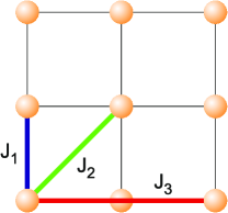
We address two-dimensional Heisenberg model with spin on the square lattice, see Fig. 2. The Hamiltonian of the model reads
| (1) |
where , denotes NN (nearest neighbor) bonds, denotes NNN (next-nearest neighbor) bonds and denotes NNNN (next-to-next-nearest neighbor) bonds of the square lattice sites .
Expression 1 provides the minimal possible model, since quantum (and classical in the limit ) helices appear starting from “”-level of multi-exchange Heisenberg Hamiltonian. In other words, yet does not lead to a helical state.
We first briefly remind the classical limit of the problem. For classical spins in 2D any order, commensurate or incommensurate, can be set by the simple ansatz (plane spiral), [82, 83, 84] see also symmetry analysis in Ref. [85].
| (2) |
where and are in-plane orthogonal unit vectors. For fixed values of exchanges the spin structure is determined by the energy minimization with respect to control point position.
First of all this means that only long-range order (LRO) is realized in the classical limit, no short-range order (SRO), that is no spin liquid. The relation 2 means -function-like spin-spin correlation functions.
In the quantum case under consideration (), we underline, average site spin is zero
| (3) |
and the spin order is defined by the structure factor which is usually a complicated continuous function of momentum in the Brillouin zone with more or less pronounced maximum.
2.2 The method
We use the so called spherically symmetric self-consistent approach for spin-spin Green’s functions (SSSA). [64, 65, 66, 67, 68, 20]
SSSA conserves all the symmetries of the problem: the -spin symmetry and the translational invariance and allows:
i. to hold the Marshall and Mermin–Wagner theorems (in our case it means in particular that average site spin is zero at any temperature, see Eq. 3).
ii. to analyse at the states with and without long-range order
iii. to find in the wide temperature range: the spin-excitation spectrum , the dynamic susceptibility and the structure factor .
Note that SSSA always leads to a singlet state. At and under Marshall’s theorem conditions the approach does not contradict the theorem. At and arbitrary exchange couplings , , the approach is consistent with Mermin-Wagner theorem. Note also we don’t know any descriptions of broken-symmetry states, e.g., box or columnar spin liquid states as well as fractionalized excitations by SSSA or related approaches. [86]
The core of the SSSA is comprised by the chain of equations for spin Green’s function
| (4) |
truncated at the second step.
The spherical symmetry is maintained , , average cite spin is zero , three branches of spin excitations are degenerate with respect to . The spin order (short- or long-range) is characterized by spin–spin correlation functions. The long-range order possible only for is featured by spin–spin correlation non-vanishing at infinity. Hereafter we focus on .
The -dependent Green’s function
| (5) |
acquires the form
| (6) |
see Ref. [87] for supplementary details and bulky expressions for -depending and the spin excitations spectrum . Here the damping of spin excitation is neglected (“quasielastic” approximation).
Lattice sums in (8) have the form:
here
| (9) |
where , are radius vectors of nearest, next-nearest or next-to-next-nearest neighbor sites; , and implies .
The coefficients in the expression for are:
| (10) |
In (7), (10) , where the sum is take over the cites of the -th coordination sphere and is the number that cites. For 2D square lattice . In eq. (9), are correlators with vertex corrections; we use here the one vertex approximation (see, e.g., [87],[88]).
In other words, SSSA truncates the equation-of-motion hierarchy for the spin-spin Green’s function after the second level, yielding ultimately lorentzian spin excitations, eq. 6, with self-consistently determined pole weights and positions .
For model the Green’s function depend on the correlators for eight coordination spheres (we use the definition the first coordination sphere as the manifold of the nearest neighbors, the second – as the manifold of next nearest neighbors and so on). Moreover, must satisfy the spin constraint, the on-site correlator . All the correlators can be evaluated self-consistently in terms of . So there are nine conditions
| (11) |
where , ) belongs to -th coordination spheres, the structure factor
| (12) |
The system of self-consistent equations 6–12 is analyzed numerically. Hereafter all the energy-related parameters are set in the units of .
The structure factor landscape saturates at . So all the foregoing results have been obtained at low temperature .
Indeed, Green’s-function method has its limitations. In the case of better investigated parent J1-J2 square-lattice model SSSA in its standard simple realization is known to overestimate the borders of the spin-liquid region (see Fig.1 from [27]) compared to results of exact diagonalization, density-matrix renormalization group [29], and functional renormalization group [58]. Here we use the variant of SSSA, where we neglect the spin-spin excitations damping and involve only one vertex correction. Note that in a number of previous works this limitation was partially eliminated and fine tuning of the approach was elaborated including damping, many vertices approximation, Zwanzig–Mori projection approach [68, 87, 89]. It was shown in particular that under the tuning of the SSSA spin-liquid area is close to that of modern numerical methods. Nevertheless, the quantitative picture remains stable.
2.3 Results and discussion
In the classical limit the structure factor is always -function like (see Eq. 2). This means that there is only one unique wave vector defining spin order (apart from symmetry equivalent points in the Brillouin zone).
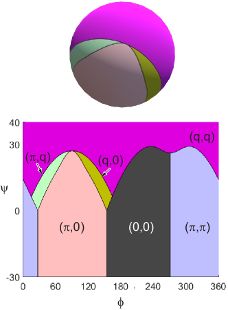
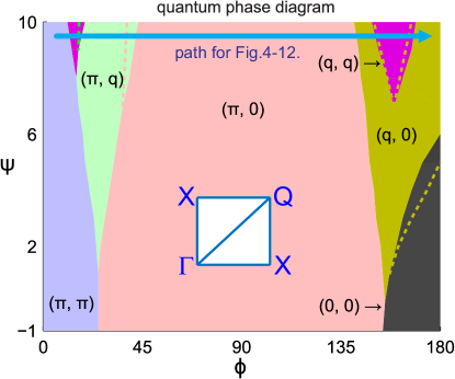
In the quantum case the structure factor is usually a smooth complicated continuous function of momentum . Nevertheless at not very high temperatures local spin order can be distinguished by the positions of the structure factor maxima (see Fig. 3).
The most interesting situation corresponds to continuous degeneracy of the structure factor maxima: in this case they merge into the curve in the -space (this is hardly possible in the classical limit). Sometimes this curve is topologically equivalent to a circle, then we can discuss the circular quantum structures.
We underline, that the last picture is natural only for the strongly frustrated model. For example such continuous degeneracy does not appear in the square lattice model: the third frustrating exchange is necessary.
Note that the adopted quantum approach treats the spin liquid rather coarsely, being based generally on two-site spin-spin correlators. There are numerous works, where at zero and extremely low temperatures phases of a more complex structure (e.g. columnar phase, spin nematic, vortex crystal, valence-bond crystal,…) are mentioned, determined by higher-order correlators (usually four-cite). The nomenclature of such states is extensive, and the related literature is vast (see e.g. [90, 91] for the review). Here we detect a noticeable maximum of the structural factor (and the corresponding minimum of the spin gap). Against this background, correlators of higher orders will only lead to the appearance of small ripples on the main structure. Moreover, as the temperature rises, the “fine structure” blurs much faster than the main peaks.
Basically, it is possible to get more complex structure (columnar, nematic, etc) in the SSSA-like approach. Then one should start from the states not of a single cite, but of a block like it was done, e.g. in Ref. [92]. This is the subject for the forthcoming investigations.
2.3.1 Phase diagram: general properties
In model the norm is irrelevant for short-range order and the phase diagram. So the kind of “globe” parametrisation is convenient
| (13) | |||||
Here , and is the standard spherical angle. This choice improves the observables readability.
The physics of the problem depends only on the relative magnitude of the coupling constants, so energy scale may be freely chosen. The standard choice in the field is . Nevertheless while passing the areas the euclidean norm of the vector is more convenient.
Like on the earth globe, there is a “no man’s land” at the “poles” (, that is , ), where there is almost nothing interesting and experimentally relevant on the phase diagram. The most intriguing are the “equatorial” latitudes of the “north” hemisphere, , . One can see, that this region, depicted in Fig. 3, is the most frustrated.
We choose the trajectory on the phase diagram, see thick blue arrow line (, that is ) in Fig. 3, that passes the following states:
-
•
AFM with structure factor maxima at ;
-
•
stripe — , in the classical limit it would be alternating stripes along a lattice with spins up and down;
-
•
FM ;
-
•
helicoid ;
-
•
helicoid ;
-
•
helicoid .
The last three in the classical limit would be spin helices rotating along one of the axis or along the diagonal of the square lattice. In Fig. 3 and hereafter we label the local orders with one of the equivalent points .
Below evolution of the structure factor and the spin excitations spectra along the trajectory is investigated. We focus on the transitions corresponding to local order changes. The borders of different local orders are well-defined and correspond to changes of structure factor maxima.
The situation in the “depth” of each phase is more or less clear, at least qualitatively. But the transitions between definite spin-liquid local orders is much more intriguing. Note that the physical picture here is some sense similar to liquid-liquid transitions. [93, 94, 95, 96, 97, 98]
We are to remind some general properties of the spectrum. [65, 66, 67, 68] The spin gap is always closed at trivial point at any temperature. At it might be closed at nontrivial points in the Brilloin zone with -peak of structure factor at the same point. These means the corresponding long-range order (AFM, FM, stripe or helical). At spin-liquid states are also possible.
We are interested in the case of , when the long-range order is always absent, but the short-range order remains pronounced and complicated. The local order is defined by the structure factor maximum and the spectrum minimum at nontrivial points.
2.3.2 From AFM via two helices to stripe
From via to .
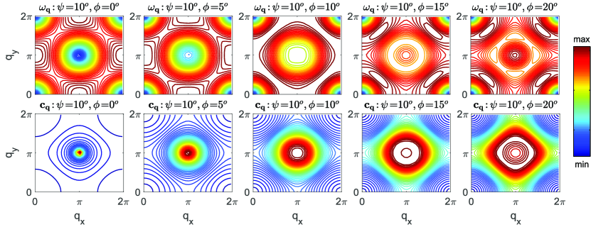
The spectrum and structure factor evolution in this domain is shown in Fig. 4. We have chosen the frame of reference for the Brillouin zone . In this case the AFM maxima are located in the centre of the Brillouin zone.
The first figure-column in Fig. 4 just corresponds to AFM with the sharp maximum of the structure factor and the local minimum of the spin excitations spectrum at the AFM point . For large enough () the short-range order becomes clearly stripe-like (see Fig. 6) with maximum and minimum at the stripe point and the equivalent ones. The half-width of the mentioned maxima in these limits defines the correlation length correspondingly for AFM and stripe order.
In between these limits evolves smoothly and its peak becomes much wider implying the correlation length’s diminishing, see the second figure-column in Fig. 4.
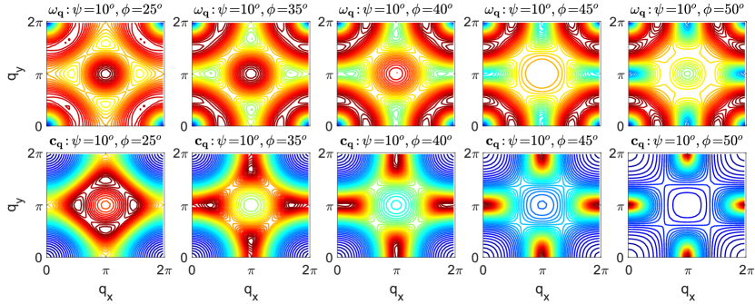

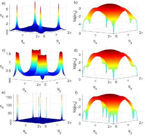
At higher (that is ) the top of the peak starts collapsing down and the peak acquires “volcanic” shape, see the evolution between second and fifth figure-columns in Fig. 4.
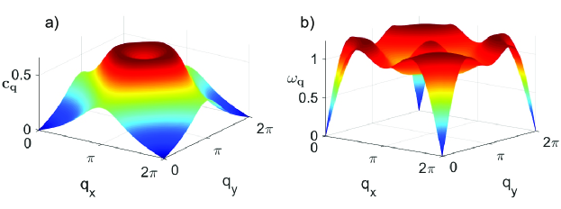
The form of the structure factor defines the symmetry and the structure of the underlying quantum state. Thus, we get the desired circular quantum states, with the maxima forming the circle structure centered at see Fig. 5. This indicates local order of the antiferromagnetic isotropical helix [58, 59]. The continuous circular degeneracy can be treated as the quantum superposition of incommensurate spiral states propagating in all directions.
The in Fig. 5 with the volcanic shape being imaginatively squeezed to the point acquires purely AFM local order. The nonzero diameter of the crater is the incommensurability parameter for the degenerate set of helices and the width of the walls of the crater defines the correlation length.
From to .
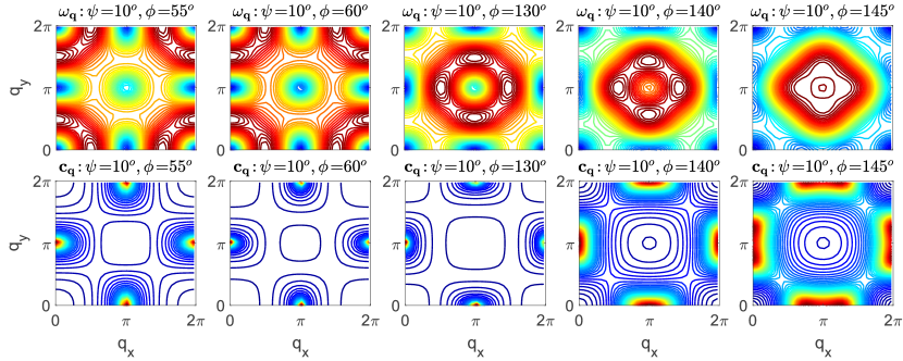
The spectrum and structure factor evolution in this domain is shown in Fig. 6. With the growth of (that is ) circular “volcanic” structure of acquires the four-fold modulation that finally transforms into four distinct peaks. The last is the quantum stripe state: the superposition of local stripes along perpendicular directions, see Fig. 7.
2.3.3 From stripe via two helices to FM
The spectrum and structure factor evolution in this domain is shown in Fig. 8-9. We remind that the frame of reference for the Brillouin zone here is .
In the range the local order is stripe-like. The correlation length is maximal for and decays on both sides. After leaving the stripe region () the peaks of split and the local order acquires helical structure.
Correspondingly, the excitation spectrum undergoes the splitting of local minima and transforms from “spider” to “squid” shape.
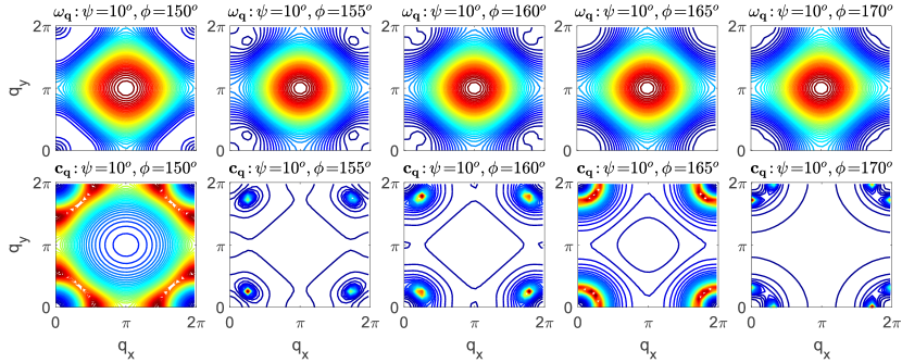
Structure factor maximum underdoes similar splitting, that can be interpreted as the crossover to the incommensurate helical state, more exactly, to the quantum superposition of several such states.
Reentrance from to .
From via towards .
In contrast to the classical limit, there exists the island of helical local order with the subsequent reentrance to helical local order.
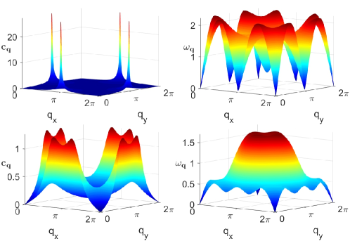
The complex helix state, that in contrast to AFM circular structure, see Fig. 5, is to be labeled as FM circular structure, appears in the borderland (see the fourth figure-column in Fig. 10). Similar observation have been made recently in Ref. [3] using purely numerical tools (quantum Monte-Carlo simulation).
The correlation length shows nontrivial nonmonotonic evolution while passing from purely to purely helix. It dramatically drops in the borderland being sufficiently large on both sides, as it is seen from the evolution of the structure factor peaks in Fig. 11.
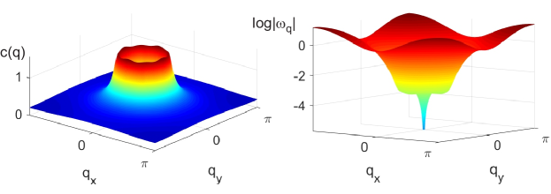
From the first glance, it is difficult to detect a circular state from Fig. 11. In the FM region returning to the standard frame of reference for the Brillouin zone is natural. This is done in Fig. 12, where FM circular shape of the structure factor becomes obvious.
The “flower” spectrum on the right in Fig. 12 requires additional explanation. The spectrum has two distinct parts — the flower itself and the stem. The stem is determined by the spin gap at the trivial zero point . This gap is closed at any temperature for any set of exchange parameters.
The structure factor has a peak at zero point only in the region of purely FM short-range order not discussed here. In all other cases, particularly for helix zero spin gap at trivial point does not generate corresponding peak. In the bottom row in Fig. 11 the side peaks near the trivial point are generated by spectrum narrow dips at points being the traces of quantum helical order.
Let us mention that the circle-like vanishing spin gap, or in other words, the circle-like maxima is the precursor of Brazovskii transition. [99]
Note in addition, that the correlation length of the FM circular state is much larger than the correlation length of the AFM circular state (compare Fig. 5 and Fig. 11).
3 Conclusions
To conclude, we have considered the topical case of the systems with multiple frustrating exchanges — two-dimensional Heisenberg model. Many important results for this problem are scattered over the localized islands of parameters, while areas in between still require investigation.
We use the spherically symmetric self-consistent approach for spin-spin Green’s functions. It conserves all the key symmetries of the problem (the -spin symmetry and the translational invariance) and strictly holds the characteristic limitation of low-dimensionality.
Note that purely analytical approaches (e.g. spin waves), in 2D should be used with caution (see [91] for a recent review). Generally accepted results here are still absent, and as a rule, analytical approach serves as a basis for further numerical studies. Let us underline that the problem at hand (detailed investigation of the large area of parameters) is resource consuming for direct numerical simulation: the frustration especially multi-exchange increases the well-known “sign problem” and there are also system size limitations. The method we use here allows to bypass these problems with the cost of some uncertainty related to the accuracy of multi-spin Greens-function approximation and to obtain in a reasonable time a physical picture in a very wide range of parameters for a moderate amount of processor-hours.
To be more specific, the evolution of a spin fluid between ferromagnetic and antiferromagnetic short-range order structures has been studied in the present work. We have found not only the structure factor but also the spin excitations spectra. It should be noted that recently circular structures have been detected by numerical methods for both ferromagnetic and antiferromagnetic signs of the first exchange [3, 58, 59]. We reproduce quantitatively most of the results from the mentioned papers. An isotropic FM helicoid was obtained in [3] for parameters , , (in our notations) and the SSSA approach reproduces this result. Similarly, SSSA reproduces Fig. 7 of [58] and Fig. 1(b-e) of [59].
The structure factor and the spin excitations spectra (in particular, the circular structures) were investigated here on the line (). However, our calculations show that in the entire range (), circular structures also appear.
We believe that our investigation in the framework of a physically transparent approach, combining a large number of limiting cases, complements and enriches this picture. The results obtained can be further refined in the most interesting areas by direct numerical methods.
It should be added that in the considered case of low but nonzero temperature, the spin state for any set of parameters is a singlet spin-liquid without long-range order. Our consideration refines the structures of a circular form — quantum helical isotropical states.
The circular state is a continuous quantum superposition of helical states; the manifold of helices directions fills the circle-like curve. The token of a circular state is a tube-like form of and the circle-like manifold of spectrum local minima. These key features enriched with traditional and parts lead to the zoo of peculiar spectra and structure factors.
Finally, we have investigated wide areas in the phase diagram when one local order state of spin-liquid transforms into another one. The nontrivial circular states are located just in the borderlands.
4 Acknowledgments
This work was supported by the Russian Foundation for Basic Research (project No. 19-02-00509). We express our gratitude to Russian Science Foundation (project No. 18-12-00438) for support of the numerical calculations. This work was carried out using supercomputers at Joint Supercomputer Center of the Russian Academy of Sciences (JSCC RAS), the Ural Branch of RAS, and the federal collective usage center Complex for Simulation and Data Processing for Mega-science Facilities at NRC “Kurchatov Institute”, http://ckp.nrcki.ru/.
References
References
- [1] Balents L 2010 Nature 464 199
- [2] Kawamura H 2011 J. Phys.: Conf. Ser. 320 012002 ISSN 1742-6596
- [3] Seabra L, Sindzingre P, Momoi T and Shannon N 2016 Phys. Rev. B 93 085132
- [4] Danu B, Nambiar G and Ganesh R 2016 Phys. Rev. B 94 094438
- [5] Hu A Y and Wang H Y 2017 Sci. Rep. 7 10477 ISSN 2045-2322
- [6] Ferrari F, Bieri S and Becca F 2017 Phys. Rev. B 96 104401
- [7] Buessen F L, Hering M, Reuther J and Trebst S 2018 Phys. Rev. Lett. 120 057201
- [8] Bishop R F and Li P H Y 2018 J. Phys.: Conf. Ser. 1041 012001 ISSN 1742-6596
- [9] McGrouther D, Lamb R J, Krajnak M, McFadzean S, McVitie S, Stamps R L, Leonov A O, Bogdanov A N and Togawa Y 2016 New J. Phys. 18 095004 ISSN 1367-2630
- [10] Zhang X, Xia J, Zhou Y, Liu X, Zhang H and Ezawa M 2017 Nat. Commun. 8 1717 ISSN 2041-1723
- [11] Sutcliffe P 2017 Phys. Rev. Lett. 118 247203
- [12] Leonov A O and Mostovoy M 2017 Nat. Commun. 8 14394 ISSN 2041-1723
- [13] Liang J J, Yu J H, Chen J, Qin M H, Zeng M, Lu X B, Gao X S and Liu J M 2018 New J. Phys. 20 053037 ISSN 1367-2630
- [14] Hickey C, Cincio L, Papić Z and Paramekanti A 2017 Phys. Rev. B 96 115115
- [15] Claassen M, Jiang H C, Moritz B and Devereaux T P 2017 Nat. Commun. 8 1192 ISSN 2041-1723
- [16] Yao N Y, Zaletel M P, Stamper-Kurn D M and Vishwanath A 2018 Nat. Phys. 14 405–410 ISSN 1745-2481
- [17] al Wahish A, O’Neal K R, Lee C, Fan S, Hughey K, Yokosuk M O, Clune A J, Li Z, Schlueter J A, Manson J L, Whangbo M H and Musfeldt J L 2017 Phys. Rev. B 95 104437
- [18] Belemuk A M, Chtchelkatchev N M and Mikheyenkov A V 2014 Phys. Rev. A 90 023625
- [19] Belemuk A M, Chtchelkatchev N M, Mikheyenkov A V and Kugel K I 2017 Phys. Rev. B 96 094435
- [20] Mikheenkov A V, Valiulin V E, Shvartsberg A V and Barabanov A F 2018 J. Exp. Theor. Phys. 126 404–416 ISSN 1090-6509
- [21] Belemuk A M, Chtchelkatchev N M, Mikheyenkov A V and Kugel K I 2018 New J. Phys. 20 063039
- [22] Wietek A and Läuchli A M 2017 Phys. Rev. B 95 035141
- [23] Ling C D, Allison M C, Schmid S, Avdeev M, Gardner J S, Wang C W, Ryan D H, Zbiri M and Söhnel T 2017 Phys. Rev. B 96 180410
- [24] Manson J L, Brambleby J, Goddard P A, Spurgeon P M, Villa J A, Liu J, Ghannadzadeh S, Foronda F, Singleton J, Lancaster T, Clark S J, Thomas I O, Xiao F, Williams R C, Pratt F L, Blundell S J, Topping C V, Baines C, Campana C and Noll B 2018 Sci. Rep. 8 4745 ISSN 2045-2322
- [25] Chandra P, Coleman P and Larkin A I 1990 Phys. Rev. Lett. 64(1) 88–91
- [26] Chubukov A 1991 Phys. Rev. B 44(1) 392–394
- [27] Siurakshina L, Ihle D and Hayn R 2001 Phys. Rev. B 64(10) 104406
- [28] Mambrini M, Läuchli A, Poilblanc D and Mila F 2006 Phys. Rev. B 74(14) 144422
- [29] Jiang H C, Yao H and Balents L 2012 Phys. Rev. B 86(2) 024424
- [30] Bauer D V and Fjærestad J O 2017 Phys. Rev. B 96 165141
- [31] Iqbal Y, Muller T, Ghosh P, Gingras M J P, Jeschke H O, Rachel S, Reuther J and Thomale R 2018 arXiv:1802.09546 [cond-mat]
- [32] Huang S X, Chen F, Kang J, Zang J, Shu G J, Chou F C and Chien C L 2016 New J. Phys. 18 065010 ISSN 1367-2630
- [33] Messio L, Bieri S, Lhuillier C and Bernu B 2017 Phys. Rev. Lett. 118 267201
- [34] Ye M and Chubukov A V 2017 Phys. Rev. B 96 140406
- [35] Tranquada J M 2007 Neutron scattering studies of antiferromagnetic correlations in cuprates Handbook of High-Temperature Superconductivity ed Schrieffer J R and Brooks J S (Springer New York) pp 257–298 ISBN 978-0-387-35071-4, 978-0-387-68734-6
- [36] Plakida P N 2010 Theoretical models of high-Tc superconductivity High-Temperature Cuprate Superconductors (Springer Series in Solid-State Sciences no 166) (Springer Berlin Heidelberg) pp 377–478 ISBN 978-3-642-12632-1, 978-3-642-12633-8
- [37] Melzi R, Carretta P, Lascialfari A, Mambrini M, Troyer M, Millet P and Mila F 2000 Phys. Rev. Lett. 85 1318–1321
- [38] Melzi R, Aldrovandi S, Tedoldi F, Carretta P, Millet P and Mila F 2001 Phys. Rev. B 64 024409
- [39] Rosner H, Singh R R P, Zheng W H, Oitmaa J and Pickett W E 2003 Phys. Rev. B 67 014416
- [40] Kageyama H, Kitano T, Oba N, Nishi M, Nagai S, Hirota K, Viciu L, Wiley J B, Yasuda J, Baba Y, Ajiro Y and Yoshimura K 2005 J. Phys. Soc. Jpn. 74 1702–1705
- [41] Vasala S, Avdeev M, Danilkin S, Chmaissem O and Karppinen M 2014 J. Phys.: Condens. Matter 26 496001 ISSN 1361-648X
- [42] Kaul E E, Rosner H, Shannon N, Shpanchenko R V and Geibel C 2004 J. Magn. Magn. Mater. 272–276, Part 2 922–923 ISSN 0304-8853
- [43] Skoulatos M, Goff J, Shannon N, Kaul E, Geibel C, Murani A, Enderle M and Wildes A 2007 J. Magn. Magn. Mater. 310 1257–1259 ISSN 0304-8853
- [44] Carretta P, Filibian M, Nath R, Geibel C and King P J C 2009 Phys. Rev. B 79 224432
- [45] Skoulatos M, Goff J P, Geibel C, Kaul E E, Nath R, Shannon N, Schmidt B, Murani A P, Deen P P, Enderle M and Wildes A R 2009 Europhys. Lett. 88 57005 ISSN 0295-5075, 1286-4854
- [46] Tsirlin A A and Rosner H 2009 Phys. Rev. B 79 214417
- [47] Tsirlin A A, Schmidt B, Skourski Y, Nath R, Geibel C and Rosner H 2009 Phys. Rev. B 80 132407
- [48] Bossoni L, Carretta P, Nath R, Moscardini M, Baenitz M and Geibel C 2010 Phys.Rev. B 83 014412
- [49] Nath R, Tsirlin A A, Rosner H and Geibel C 2008 Phys. Rev. B 78 064422
- [50] Feldkemper S, Weber W, Schulenburg J and Richter J 1995 Phys. Rev. B 52 313–323
- [51] Feldkemper S and Weber W 1998 Phys. Rev. B 57 7755–7766
- [52] Manaka H, Koide T, Shidara T and Yamada I 2003 Phys. Rev. B 68 184412
- [53] Kasinathan D, Kyker A B and Singh D J 2006 Phys. Rev. B 73 214420
- [54] Tsirlin A A, Janson O, Lebernegg S and Rosner H 2013 Phys. Rev. B 87
- [55] Sindzingre P, Seabra L, Shannon N and Momoi T 2009 J. Phys.: Conf. Ser. 145 012048 ISSN 1742-6596
- [56] Sindzingre P, Shannon N and Momoi T 2010 J. Phys.: Conf. Ser. 200 022058 ISSN 1742-6596 cal(ED) J1-J2-J3 AFM-AFM-AFM, FM-AFM-AFM
- [57] Feldner H, Cabra D C and Rossini G L 2011 Phys. Rev. B 84(21) 214406
- [58] Reuther J, Wölfle P, Darradi R, Brenig W, Arlego M and Richter J 2011 Phys. Rev. B 83(6) 064416
- [59] Iqbal Y, Ghosh P, Narayanan R, Kumar B, Reuther J and Thomale R 2016 Phys. Rev. B 94(22) 224403
- [60] Oitmaa J 2017 Phys. Rev. B 95 014427
- [61] Schecter M, Syljuåsen O F and Paaske J 2017 Phys. Rev. Lett. 119 157202
- [62] Tymoshenko Y, Onykiienko Y, Müller T, Thomale R, Rachel S, Cameron A, Portnichenko P, Efremov D, Tsurkan V, Abernathy D, Ollivier J, Schneidewind A, Piovano A, Felea V, Loidl A and Inosov D 2017 Phys. Rev. X 7 041049
- [63] Wang L and Sandvik A W 2017 arXiv:1702.08197 [cond-mat]
- [64] Kondo J and Yamaji K 1972 Prog. Theor. Phys. 47 807–818 ISSN 0033-068X, 1347-4081
- [65] Shimahara H and Takada S 1991 J. Phys. Soc. Jpn. 60 2394–2405
- [66] Barabanov A F and Beresovsky V M 1994 J. Phys. Soc. Jpn. 63 3974–3982
- [67] Härtel M, Richter J, Götze O, Ihle D and Drechsler S L 2013 Phys. Rev. B 87 054412
- [68] Mikheyenkov A V, Shvartsberg A V, Valiulin V E and Barabanov A F 2016 J. Magn. Magn. Mater. 419 131–139 ISSN 0304-8853
- [69] Li T, Becca F, Hu W and Sorella S 2012 Phys. Rev. B 86 075111 the J1-J2 RVB Schwinger bosons
- [70] Wang L and Sandvik A W 2018 Phys. Rev. Lett. 121 107202
- [71] Shannon N, Schmidt B, Penc K and Thalmeier P 2004 Eur. Phys. J. B 38 599–616 ISSN 1434-6028, 1434-6036
- [72] Shannon N, Momoi T and Sindzingre P 2006 Phys. Rev. Lett. 96 027213
- [73] Sindzingre P, Shannon N and Momoi T 2007 J. Magn. Magn. Mater. 310 1340–1342 ISSN 0304-8853
- [74] Schmidt B, Shannon N and Thalmeier P 2007 J. Phys.: Condens. Matter 19 145211 ISSN 0953-8984, 1361-648X
- [75] Schmidt B, Shannon N and Thalmeier P 2007 J. Magn. Magn. Mater. 310 1231–1233 ISSN 0304-8853
- [76] Viana J R and de Sousa J R 2007 Phys. Rev. B 75 052403
- [77] Shindou R and Momoi T 2009 Phys. Rev. B 80 064410
- [78] Härtel M, Richter J, Ihle D and Drechsler S L 2010 Phys. Rev. B 81 174421
- [79] Dmitriev D V, Krivnov V Y and Ovchinnikov A A 1997 Phys. Rev. B 55 3620–3626
- [80] Richter J, Lohmann A, Schmidt H J and Johnston D C 2014 J. Phys.: Conf. Ser. 529 012023 ISSN 1742-6596
- [81] Ren Y Z, Tong N H and Xie X C 2014 J. Phys.: Condens. Matter 26 115601 ISSN 0953-8984, 1361-648X
- [82] Luttinger J M and Tisza L 1946 Phys. Rev. 70 954–964
- [83] Villain J 1977 Journal de Physique 38 385–391 ISSN 0302-0738
- [84] Misguich G and Lhuillier C 2005 Two-dimensional quantum antiferromagnets Frustrated Spin Systems (World Scientific) pp 229–306 ISBN 978-981-256-091-9
- [85] Messio L, Lhuillier C and Misguich G 2011 Phys. Rev. B 83 184401
- [86] Hermele M, Senthil T and Fisher M P A 2005 Phys. Rev. B 72(10) 104404
- [87] Barabanov A F, Mikheyenkov A V and Shvartsberg A V 2011 Theor. Math. Phys. 168 1192–1215 ISSN 0040-5779, 1573-9333
- [88] Barabanov A F, Maksimov L A and Mikheyenkov A V 2003 Spin polaron in the cuprate superconductors: Interpretation of the ARPES results Spectroscopy of High-Tc Superconductors ed Plakida N M (London: Taylor & Francis) pp 1–96 ISBN 9780415288088
- [89] Barabanov A F, Mikheyenkov A V and Kozlov N A 2015 JETP Lett. 102 301–306 ISSN 0021-3640, 1090-6487
- [90] Diep H T (ed) 2013 Frustrated Spin Systems 2nd ed (Singapore: World Scientific, Singapore)
- [91] Schmidt B and Thalmeier P 2017 Phys. Rep. 703 1–59
- [92] Barabanov A F, Maksimov L A and Mikheyenkov A V 1989 J. Phys.: Condens. Matter 1 10143–10151 ISSN 0953-8984 URL http://iopscience.iop.org/0953-8984/1/50/015
- [93] Katayama Y, Mizutani T, Utsumi W, Shimomura O, Yamakata M and Funakoshi K i 2000 Nature 403 170
- [94] Brazhkin V V 2002 New kinds of phase transitions: transformation in disordered substances vol 81 (Springer Science & Business Media)
- [95] Ryltsev R E and Chtchelkatchev N M 2013 Phys. Rev. E 88(5) 052101
- [96] Ryltsev R E and Chtchelkatchev N M 2017 Soft Matter 13(29) 5076–5082
- [97] Mitrea D M, Cika J A, Stanley C B, Nourse A, Onuchic P L, Banerjee P R, Phillips A H, Park C G, Deniz A A and Kriwacki R W 2018 Nat Commun 9 842
- [98] Woutersen S, Ensing B, Hilbers M, Zhao Z and Angell C A 2018 Science 359 1127–1131
- [99] Brazovskii S 1975 Soviet Journal of Experimental and Theoretical Physics 41 85