Tree-structured multi-stage principal component analysis (TMPCA): theory and applications

Abstract

A PCA based sequence-to-vector (seq2vec) dimension reduction method for the text classification problem, called the tree-structured multi-stage principal component analysis (TMPCA) is presented in this paper. Theoretical analysis and applicability of TMPCA are demonstrated as an extension to our previous work (Su ., ). Unlike conventional word-to-vector embedding methods, the TMPCA method conducts dimension reduction at the sequence level without labeled training data. Furthermore, it can preserve the sequential structure of input sequences. We show that TMPCA is computationally efficient and able to facilitate sequence-based text classification tasks by preserving strong mutual information between its input and output mathematically. It is also demonstrated by experimental results that a dense (fully connected) network trained on the TMPCA preprocessed data achieves better performance than state-of-the-art fastText and other neural-network-based solutions.

1 Introduction

In natural language processing (NLP), dimension reduction is often required to alleviate the so-called “curse of dimensionality” problem. This occurs when the numericalized input data are in a sparse high-dimensional space (Bengio ., 2003). Such a problem partly arises from the large size of vocabulary and partly comes from the sentence variations with similar meanings. Both contribute to high-degree data pattern diversity, and a high dimensional space is required to represent the data in a numerical form adequately. Due to the ever-increasing data in the Internet nowadays, the language data become even more diverse. As a result, previously well-solved problems such as text classification (TC) face new challenges (Zhang ., 2015; Mirńczuk  Protasiewicz, 2018). An effective dimension reduction technique remains to play a critical role in tackling these challenges. The new dimension reduction solution should satisfy the following criteria:

• Reduce the input dimension

• Retain the input information

More specifically, dimension reduction technique should maximally preserve the input information given the limited dimension available for representing the input data. Different classifiers will perform differently given the same input data. Our objective is not to find such best performing classifiers, but to propose a dimension reduction technique that can facilitate the following classification process.

There are many ways to reduce the language data to a compact form. The most popular ones are the neural network (NN) based techniques (Zhang ., 2015; Moraes ., 2013; Ghiassi ., 2013; Araque ., 2017; T. Chen ., 2017; Joulin ., 2017). In Bengio . (2003), each element in an input sequence is first numericalized/vectorized as a vocabulary-sized one-hot vector with bit “1” occupying the position corresponding to the index of that word in the vocabulary. This vector is then fed into a trainable dense network called the embedding layer. The output of the embedding layer is another vector of a reduced size. In Mikolov . (2013), the embedding layer is integrated into a recurrent NN (RNN) used for language modeling so that the trained embedding layer can be applied to more generic language tasks. Both Bengio . (2003) and Mikolov . (2013) conduct dimension reduction at the word level. Hence, they are called word embedding methods. These methods are limited in modeling “sequences of words”, which is called the sequence-to-vector (seq2vec) problem, for two reasons. First, word embedding is trained on some particular dataset using the stochastic gradient descent method, which could lead to overfitting (Lai ., 2016) easily. Second, the vector space obtained by word embedding is still too large, it is desired to convert a sequence of words to an even more compact form.

Among non-neural-network dimension reduction methods (Deerwester ., 1990; Kontopoulos ., 2013; Wei ., 2015; Ye ., 2009; Uysal, 2016; K. Chen ., 2016), the principal component analysis (PCA) is a popular one. In Deerwester . (1990), sentences are first represented by vocabulary-sized vectors, where each entry holds the frequency of a particular word in the vocabulary. Each sentence vector forms a column in the input data matrix. Then, the PCA is used to generate a transform matrix for dimension reduction on each sentence. Although the PCA has some nice properties such as maximum information preservation (Linsker, 1988) between its input and output under certain constraints, we will show later that its computational complexity is exceptionally high as the dataset size becomes large. Furthermore, most non-RNN-based dimension reduction methods, such as Deerwester . (1990); Uysal (2016); K. Chen . (2016), do not consider the positional correlation between elements in a sequence but adopt the “bag-of-word” (BoW) representation. The sequential information is lost in such a dimension reduction procedure.

To address the above-mentioned shortcomings, a novel technique, called the tree-structured multi-stage PCA (TMPCA), was proposed in Su . (). The TMPCA method has several interesting properties as summarized below.

1. High efficiency. Reduce the input data dimension with a small model size at low computational complexity.

2. Low information loss. Maintain high mutual information between an input and its dimension-reduced output.

3. Sequential preservation. Preserve the positional relationship between input elements.

4. Unsupervised learning. Do not demand labeled training data.

5. Transparent mathematical properties. Like PCA, TMPCA is linear and orthonormal, which makes the mathematical analysis of the system easier.

These properties are beneficial to classification tasks that demand low-dimensional yet highly informative data. It also relaxes the burden of data labeling in the training stage. So TMPCA can be used as a preprocessing stage for classification problems, a complete classification framework using TMPCA is shown in figure below where the training TMPCA does not demand labels:

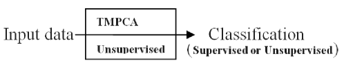
Figure 1: Integration of TMPCA to classification problems.

In this work, we present the TMPCA method and apply it to several text classification problems such as spam email detection, sentiment analysis, news topic identification, etc. This work is an extended version of Su . (). As compared with Su . (), most material in Sec. 3 and Sec. 4 is new. We present more thorough mathematical treatment in Sec. 3 by deriving the function of the TMPCA method and analyzing its properties. Specifically, the information preserving property of the TMPCA method is demonstrated by examining the mutual information between its input and output. Also, we provide more extensive experimental results on large text classification datasets to substantiate our claims in Sec. 4.

The rest of this paper is organized as follows. Research on text classification problems is reviewed in Sec. 2. The TMPCA method and its properties are presented in Sec. 3. Experimental results are given in Sec. 4, where we compare the performance of the TMPCA method and that of state-of-the-art NN-based methods on text classification, including fastText (Joulin ., 2017) and the convolutional-neural-network (CNN) based method (Zhang ., 2015). Finally, concluding remarks are drawn in Sec. 5.

2 Review of Previous Work on Text Classification

Text classification has been an active research topic for two decades. Its applications such as spam email detection, age/gender identification and sentiment analysis are omnipresent in our daily lives. Traditional text classification solutions are mostly linear and based on the BoW representation. One example is the naive Bayes (NB) method (Friedman ., 1997), where the predicted class is the one that maximizes the posterior probability of the class given an input text. The NB method offers reasonable performance on easy text classification tasks, where the dataset size is small. However, when the dataset size becomes larger, the conditional independence assumption used in likelihood calculation required by the NB method limits its applicability to complicated text classification tasks.

Other methods such as the support vector machine (SVM) (Moraes ., 2013; Ye ., 2009; Joachims, 1998) fit the decision boundary in a hand-crafted feature space of input texts. Finding representative features of input texts is actually a dimension reduction problem. Commonly used features include the frequency that a word occurs in a document, the inverse-document-frequency (IDF), the information gain (Uysal, 2016; K. Chen ., 2016; Salton  Buckley, 1988; Yang  Pedersen, 1997), etc. Most SVM models exploit BoW features, and they do not consider the position information of words in sentences.

The word position in a sequence can be better handled by the CNN solutions since they process the input data in sequential order. One example is the character level CNN (char-CNN) as proposed in Zhang . (2015). It represents an input character sequence as a two-dimensional data matrix with the sequence of characters along one dimension and the one-hot embedded characters along the other one. Any character exceeding the maximum allowable sequence length is truncated. The char-CNN has 6 convolutional (conv) layers and 3 fully-connected (dense) layers. In the conv layer, one dimensional convolution is carried out on each entry of the embedding vector.

RNNs offer another NN-based solution for text classification (Mirńczuk  Protasiewicz, 2018; T. Chen ., 2017). An RNN generates a compact yet rich representation of the input sequence and stores it in form of hidden states of the memory cell. It is the basic computing unit in an RNN. There are two popular cell designs: the long short-term memory (LSTM) (Hochreiter  Schmidhuber, 1997) and the gate recurrent unit (GRU) (Cho ., 2014). Each cell takes each element from a sequence sequentially as its input, computes an intermediate value, and updates it dynamically. Such a value is called the constant error carousal (CEC) in the LSTM and simply a hidden state in the GRU. Multiple cells are connected to form a complete RNN. The intermediate value from each cell forms a vector called the hidden state. It was observed in Elman (1990) that, if a hidden state is properly trained, it can represent the desired text patterns compactly, and similar semantic word level features can be grouped into clusters. This property was further analyzed in Su . (Unpublished). Generally speaking, for a well designed representational vector (i.e. the hidden state), the computing unit (or the memory cell) can exploit the word-level dependency to facilitate the final classification task.

Another NN-based model is the fastText (Joulin ., 2017). As shown in Fig. 2, it is a multi-layer perceptron composed by a trainable embedding layer, a hidden mean layer and a softmax dense layer. The hidden vector is generated by averaging the embedded word, which makes the fastText a BoW model. The fastText offers a very fast solution to text classification. It typically takes less than a minute in training a large data corpus with millions of samples. It gives the state-of-the-art performance. We would like to use it as the primary benchmarking algorithm in Sec. 4. All NN-based text classification solutions demand labeled data in training. We will present the TMPCA method, which does not need labeled training data, in the next section.

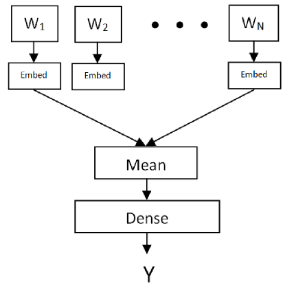
Figure 2: Illustration of the fastText model.

3 Proposed TMPCA Method

In essence, TMPCA is a tree-structured multi-stage PCA method whose input at every stage is two adjacent elements in an input sequence without overlap. The reason for every two elements rather than other number of elements is due to the computational efficiency of such an arrangement. This will be elaborated in Sec. 3.2. The block diagram of TMPCA with a single sequence $\{w_{1},...,w_{N}\}$ as its input is illustrated in Fig. 3. The input sequence length is $N$, where $N$ is assumed to be a number of the power of 2 for ease of discussion below. We will relax such a constraint for practical implementation in Sec. 4. We use $z^{s}_{j}$ to denote the $j$th element in the output sequence of stage $s$ (or equivalently, the input sequence of stage $s+1$ if such a stage exists). It is obvious that the final output $Y$ is also $z^{\text{log}_{2}N}_{1}$.

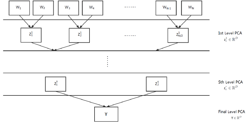
Figure 3: The Block diagram of the TMPCA method.

3.1 Training of TMPCA

To illustrate how TMPCA is trained, we use an example of a training dataset with two sequences, each of which has four numericalized elements. Each element is a column vector of size $D$, denoted as $w^{i}_{j}$, where $i$ indicates the corresponding sequence and $j$ is the position of the element in that sequence. At each stage of the TMPCA tree, every two adjacent elements without overlap are concatenated to form one vector of dimension $2D$. It serves as a sample for PCA training at that stage. Thus, the training data matrix for PCA at the first stage can be written as

$$\begin{bmatrix}(w^{1}_{1})^{T}&(w^{1}_{2})^{T}\\ (w^{1}_{3})^{T}&(w^{1}_{4})^{T}\\ (w^{2}_{1})^{T}&(w^{2}_{2})^{T}\\ (w^{2}_{3})^{T}&(w^{2}_{4})^{T}\end{bmatrix}.$$

The trained PCA transform matrix at stage $s$ is denoted as $U^{s}$. It reduces the dimension of the input vector from $2D$ to $D$. That is, $U^{s}\in\mathbb{R}^{D\times 2D}$. The training matrix at the first stage is then transformed by $U^{1}$ to

$$\begin{bmatrix}(z^{1}_{1})^{T}\\ (z^{1}_{2})^{T}\\ (z^{1}_{3})^{T}\\ (z^{1}_{4})\end{bmatrix},\quad z^{1}_{1}=U^{1}(\begin{bmatrix}w^{1}_{1}\\ w^{1}_{2}\end{bmatrix}),\quad z^{1}_{2}=U^{1}(\begin{bmatrix}w^{1}_{3}\\ w^{1}_{4}\end{bmatrix}),\quad z^{1}_{3}=U^{1}(\begin{bmatrix}w^{2}_{1}\\ w^{2}_{2}\end{bmatrix}),\quad z^{1}_{4}=U^{1}(\begin{bmatrix}w^{2}_{3}\\ w^{2}_{4}\end{bmatrix}),$$

After that, we rearrange the elements on the transformed training matrix to form

$$\begin{bmatrix}(z^{1}_{1})^{T}&(z^{1}_{2})^{T}\\ (z^{1}_{3})^{T}&(z^{1}_{4})^{T}\end{bmatrix}.$$

It serves as the training matrix for the PCA at the second stage. We repeat the training data matrix formation, the PCA kernel determination and the PCA transform steps recursively at each stage until the length of the training samples becomes 1. It is apparent that, after one-stage TMPCA, the sample length is halved while the element vector size keeps the same as $D$. The dimension evolution from the initial input data to the ultimate transformed data is shown in Table 1. Once the TMPCA is trained, we can use it to transform test data by following the same steps except that we do not need to compute the PCA transform kernels at each stage.

Table 1: Dimension evolution from the input to the output in the TMPCA method.

	Sequence length	Element vector size
Input sequence	N	D
Output sequence	1	D

3.2 Computational Complexity

We analyze the time complexity of TMPCA training in this section. Consider a training dataset of $M$ samples, where each sample is of length $N$ with element vectors of dimension $D$. To determine the PCA model for this training matrix of dimension $\mathbb{R}^{M\times ND}$, it requires $\text{O}(MN^{2}D^{2})$ to compute the covariance matrix, and $\text{O}(N^{3}D^{3})$ to compute the eigenvalues of the covariance matrix. Thus, the complexity of PCA can be written as

$$\text{O}(f_{\text{PCA}})=\text{O}\Big{(}N^{3}D^{3}+MN^{2}D^{2}\Big{)}.$$ (1)

The above equation can be simplified by comparing the value of $M$ with $ND$. We do not pursue along this direction furthermore since it is problem dependent.

Suppose that we concatenate non-overlapping $P$ adjacent elements at each stage of TMPCA. The dimension of the training matrix at stage $s$ is $M\frac{N}{P^{s}}\times PD$. Then, the total computational complexity of TMPCA can be written as

$$\text{O}(f_{\text{TMPCA}}) =\text{O}\Big{(}\sum^{\log_{P}N}_{s=1}\big{(}(PD)^{3}+M\frac{N}{P^{s}}(PD)^{2}\big{)}\Big{)},$$

$$=\text{O}\Big{(}(P^{3}\text{log}_{P}N)D^{3}+M\frac{P^{2}}{P-1}(N-1)D^{2}\Big{)}.$$ (2)

The complexity of TMPCA is an increasing function in $P$. This can be verified by non-negativity of its derivative with respect to $P$. Thus, the worst case is $P=N$, which is simply the traditional PCA applied to the entire samples in a single stage. When $P=2$, the TMPCA achieves its optimal efficiency. Its complexity is

$$\text{O}(f_{\text{TMPCA}}) =\text{O}\Big{(}8(\text{log}_{2}N)D^{3}+4M(N-1)D^{2}\Big{)},$$

$$=\text{O}\Big{(}2(\text{log}_{2}N)D^{3}+M(N-1)D^{2}\Big{)}.$$ (3)

By comparing Eqs. (3.2) and (1), we see that the time complexity of the traditional PCA grows at least quadratically with sentence length $N$ (since $P=N$) while that of TMPCA grows at most linearly with $N$.

3.3 System Function

To analyze the properties of TMPCA, we derive its system function in closed form in this section. In particular, we will show that, similar to PCA, TMPCA is a linear transform and its transformation matrix has orthonormal rows. For the rest of this paper, we assume that the length of the input sequence is $N$ $N=2^{L}$, where $L$ is the total stage number of TMPCA. The input is mean-removed so that its mean is $\bm{0}$.

We denote the element of the input sequence by $w_{j}$, where $w_{j}\in\mathbb{R}^{D}$ and $j\in\{1,...,N\}$. Then, the input sequence $X$ to TMPCA is a column vector in form of

$$X^{T}=[w^{T}_{1},\cdots,w^{T}_{N}].$$ (4)

We decompose PCA transform matrices, $U^{s}$, at stage $s$ into two equal-sized block matrices as

$$U^{s}=[U^{s}_{1},U^{s}_{2}],$$ (5)

where $U^{s}_{j}\in\mathbb{R}^{D\times D}$, and where $j\in\{1,2\}$. The output of TMPCA is $Y\in\mathbb{R}^{D}$

With notations inherited from Sections 3.1 and 3.2, we can derive the closed-form expression of TMPCA by induction (see Appendix A). That is, we have

$$Y =UX,$$ (6)

$$U =[U_{1},...,U_{N}],$$ (7)

$$U_{j} =\prod^{L}_{s=1}U^{s}_{f_{j,s}},\forall j\in\{1,...,N\}$$ (8)

$$f_{j,s} =\text{b}_{L}(j-1)_{s}+1,\forall j,s.$$ (9)

where $\text{b}_{L}(x)_{s}$ is the $s$th digit of $L$-binarized form of $x$. TMPCA is a linear transform as shown in Eq. 6. Also, since there always exist real valued eigenvectors to form the PCA transform matrix, $U$, $U_{j}$ and $\{U^{s}_{j}\}^{2}_{j=1}$ are all real valued matrices.

To show that $U$ has orthonormal rows, we first examine the properties of matrix $K=[U_{1},U_{2}]$. By setting

$$A=\prod^{L}_{s=2}U^{s}_{f_{1,s}}=\prod^{L}_{s=2}U^{s}_{f_{2,s}},$$

we obtain $K=[AU^{1}_{1},AU^{1}_{2}]$. Since matrix $[U^{1}_{1},U^{1}_{2}]$ is a PCA transform matrix, it has orthonormal rows. Denote $<\cdot>_{ij}$ as the inner product between the $i$th row and $j$th row of matrix $\cdot$, we conclude that the $<K>_{ij}=<A>_{ij}$ using the following property.

Lemma 1.

Given $K=[AB_{1},AB_{2}]$, where $[B_{1},B_{2}]$ has orthonormal rows, then $<K>_{ij}=<A>_{ij}$.

We then let

$$K^{s}_{m}=[A^{s}_{m}U^{s}_{1},A^{s}_{m}U^{s}_{2}],$$ (10)

where $s\in\{1,...,L\}$ indicates the stage, and $m\in\{1,...,\frac{N}{2^{s}}\}$, and

$$A^{s}_{m}=\prod^{L}_{k=s+1}U^{k}_{f_{m,k-s}},\mbox{ and }A^{L}_{1}=\bm{I},$$ (11)

where $\bm{I}$ is the identity matrix. At stage 1, $K^{1}_{m}=[U_{2m-1},U_{2m}]$, so $U=[K^{1}_{1},...,K^{1}_{N/2}]$. Since $<U>_{ij}=\sum^{N/2}_{m=1}<K^{1}_{m}>_{ij}$, according to 1, Eqs. (10)-(11) we have

$$<U>_{ij} =\sum^{N/2}_{m=1}<A^{1}_{m}>_{ij},$$

$$=\sum^{N/4}_{m=1}<K^{2}_{m}>_{ij}=\sum^{N/4}_{m=1}<A^{2}_{m}>_{ij},$$

$$\ldots$$

$$=<K^{L}_{1}>_{ij}=<[U^{L}_{1},U^{L}_{2}]>_{ij},$$ (12)

Thus, $U$ has orthonormal rows.

3.4 Information Preservation Property

Besides its low computation complexity, linearity and orthonormality, TMPCA can preserve the information of its input effectively so as to facilitate the following classification process. To show this point, we investigate the mutual information (Linsker, 1988; Bennasar ., 2015) between the input and the output of TMPCA.

Here, the input to the TMPCA system is modeled as

$$X=G+n,$$ (13)

where $G$ and $n$ are used to model the ground truth semantic signal and the noise component in the input, respectively. In other words, $G$ carries the essential information for the text classification task while $n$ is irrelevant to (or weakly correlated) the task. We are interested in finding the mutual information between output $Y$ and ground truth $G$.

By following the framework in Linsker (1988), we make the following assumptions:

1. $Y\sim\mathbb{N}(\bar{y},\bm{V})$;

2. $n\sim\mathbb{N}(\bm{0},\bm{B})$, where $\bm{B}=\sigma^{2}\bm{I}$;

3. $n$ is uncorrelated with $G$.

In above, $\mathbb{N}$ denotes the multivariant Gaussian density function. Then, the mutual information between $Y$ and $G$ can be computed as

$$I(Y,G)= \text{E}_{Y,G}\left(\text{ln}\frac{P(Y|G)}{P(Y)}\right),$$

$$= \text{E}_{Y,G}\left(\text{ln}\frac{\mathbb{N}(Ug,U\bm{B}U^{T})}{\mathbb{N}(\bar{y},\bm{V})}\right),$$

$$= \frac{1}{2}\text{ln}\frac{|V|}{|U\bm{B}U^{T}|}-\frac{1}{2}\text{E}_{Y,G}\left[(y-Ug)^{T}(UBU^{T})^{-1}(y-Ug)\right]$$

$$+\frac{1}{2}\text{E}_{Y,G}\left[(y-\bar{y})^{T}V^{-1}(y-\bar{y})\right],$$ (14)

where $y\in Y$, $g\in G$, and $P(\cdot)$, $|\cdot|$ and $E_{X}$ denote the probability density function, the determinant and the expectation of random variable $X$, respectively. It is straightforward to prove the following lemma,

Lemma 2.

For any random vector $X\in\mathbb{R}^{D}$ with covariance matrix $K_{x}$, the following equality holds

$$E_{X}\{(x-\bar{x})^{T}(K_{x})^{-1}(x-\bar{x})\}=D.$$

Then, based on this lemma, we can derive that

$$I(Y,G)=\frac{1}{2}\text{ln}\frac{|V|}{\sigma^{2D}}.$$ (15)

The above equation can be interpreted below. Given input signal noise $\sigma$, the mutual information can be maximized by maximizing the determinant of the output covariance matrix. Since TMPCA maximizes the covariance of its output at each stage, TMPCA will deliver an output with the largest mutual information at the corresponding stage. We will show experimentally in Section 4 that the mutual information of TMPCA is significantly larger than that of the mean operation and close to that of PCA.

4 Experiments

4.1 Datasets

We tested the performance of the TMPCA method on twelve datasets of various text classification tasks as shown in Table 2. Four of them are smaller datasets with at most 10,000 training samples. The other eight are large-scale datasets (Zhang ., 2015) with training samples ranging from 120 thousands to 3.6 millions.

Table 2: Selected text classification datasets.

	# of Class	Train Samples	Test Samples	# of Tokens
spam	2	5,574	558	14,657
sst	2	8409	1803	18,519
semeval	2	5098	2034	25,167
imdb	2	10162	500	20,892
agnews	4	120,000	7,600	188,111
sogou	5	450,000	60,000	800,057
dbpedia	14	560,000	70,000	1,215,996
yelpp	2	560,000	38,000	1,446,643
yelpf	5	650,000	50,000	1,622,077
yahoo	10	1,400,000	60,000	4,702,763
amzp	2	3,600,000	400,000	4,955,322
amzf	5	3,000,000	650,000	4,379,154

These datasets are briefly introduced below.

1. SMS Spam (spam) (Almeida ., 2011). It is a dataset collected for mobile Spam email detection. It has two target classes: “Spam” and “Ham”.

2. Stanford Sentiment Treebank (sst) (Socher ., 2013). It is a dataset for sentiment analysis. The labels are generated using the Stanford CoreNLP toolkit (Stanford, 2018). The sentences labeled as very negative or negative are grouped into one negative class. Sentences labeled as very positive or positive are grouped into one positive class. We keep only positive and negative sentences for training and testing.

3. Semantic evaluation 2013 (semeval) (Wilson ., 2013). It is a dataset for sentiment analysis. We focus on Sentiment task-A with positive/negative two target classes. Sentences labeled as “neutral” are removed.

4. Cornell Movie review (imdb) (Bo  Lee, 2005). It is a dataset for sentiment analysis for movie reviews. It contains a collection of movie review documents with their sentiment polarity (i.e., positive or negative).

5. AG’s news (agnews) (Zhang  Zhao, 2005). It is a dataset for news categorization. Each sample contains the news title and description. We combine the title and description into one sentence by inserting a colon in between.

6. Sougou news (sogou) (Zhang  Zhao, 2005). It is a Chinese news categorization dataset. Its corpus uses a phonetic romanization of Chinese.

7. DBPedia (dbpedia) (Zhang  Zhao, 2005). It is an ontology categorization dataset with its samples extracted from the Wikipedia. Each training sample is a combination of its title and abstract.

8. Yelp reviews (yelpp and yelpf) (Zhang  Zhao, 2005). They are sentiment analysis datasets. The Yelp review full (yelpf) has target classes ranging from one to five stars. The one star is the worst while five stars the best. The Yelp review polarity (yelpp) has positive/negative polarity labels by treating stars 1 and 2 as negative, stars 4 and 5 positive and omitting star 3 in the polarity dataset.

9. Yahoo! answers (yahoo) (Zhang  Zhao, 2005). It is a topic classification dataset for Yahoo’s question and answering corpus.

10. Amazon reviews (amzp and amzf) (Zhang  Zhao, 2005). These two datasets are similar to Yelp reviews but of much larger sizes. They are about Amazon product reviews.

4.2 Experimental Setup

We compare the performance of the following three methods on the four small datasets:

1. TMPCA-preprocessed data followed by the dense network (TMPCA+Dense);

2. fastText;

3. PCA-preprocessed data followed by the dense network (PCA+Dense).

For the eight larger datasets, we compare the performance of six methods. They are:

1. TMPCA-preprocessed data followed by the dense network (TMPCA+Dense);

2. fastText;

3. PCA-preprocessed data followed by the dense network (PCA+Dense);

4. char-CNN (Zhang ., 2015);

5. LSTM (an RNN based method) (Zhang ., 2015);

6. BoW (Zhang ., 2015).

Besides training time, classification accuracy and F1 macro score, we compute the mutual information between the input and the output of the TMPCA method, the mean operation (used by fastText for hidden vector computation) and the PCA method, respectively. Note that the mean operation can be expressed as a linear transform in form of

$$Y=\frac{1}{N}[\bm{I},...,\bm{I}]X,$$ (16)

where $\bm{I}\in\mathbb{R}^{D\times D}$ is the identity matrix and the mean transform matrix has $N$ $\bm{I}$’s. The mutual information between the input and the output of the mean operation can be calculated as

$$I(Y,G)=\frac{1}{2}\text{ln}\frac{|V|N^{D}}{\sigma^{2D}}.$$ (17)

For fixed noise variance $\sigma^{2}$, we can compare the mutual information of the input and the output of different operations by comparing their associated $|V|$, $|V|N^{D}$.

To illustrate the information preservation property of TMPCA across multiple stages, we compute the output energy, which is the sum of squared elements in a vector/tensor, as a percentage of its input energy, and see how the energy values decrease as the stage number becomes bigger. Such investigation is meaningful since the energy indicates signal’s variance in a TMPCA system. The variance is a good indicator of information richness. The energy percentage is an indicator of the amount of input information that is preserved after one TMPCA stage. We compute the total energy of multiple sentences by adding them together.

To numericalize the input data, we first remove the stop words from sentences according to the stop-word list, tokenize sentences and, then, stem tokens using the python natural language toolkit (NLTK). Afterwards, we use the fastText-trained embedding layer to embed the tokens into vectors of size 10. The tokens are then concatenated to form a single long vector.

In TMPCA, to ensure that the input sequence is of the same length and equal to a power of 2, we assign a fixed input length, $N=2^{L}$, to all sentences of length $N^{\prime}$. If $N^{\prime}<N$, we preprocess the input sequence by padding it to be of length $N$ with a special symbol. If $N^{\prime}>N$, we shorten the input sequence by dividing it into $N$ segments and calculating the mean of numericalized elements in each segment. The new sequence is then formed by the calculated means. The reason of dividing a sequence into segments is to ensure consecutive elements as close as possible. Then, the segmentation of an input sequence can be conducted as follows.

1. Calculate the least number of elements that each segment should have: $d=\text{floor}(N^{\prime}/N)$, where floor denotes flooring operation.

2. Then we allocate the remaining $r=N^{\prime}-dN$ elements by adding one more element to every other floor$(N/r)$ segments until there are no more elements left.

To give an example, to partition the sequence $\{w_{1},\cdots,w_{10}\}$ into four segments, we have 3, 2, 3, 2 elements in these four segments, respectively. That is, they are: $\{w_{1},w_{2},w_{3}\}$, $\{w_{4},w_{5}\}$, $\{w_{6},w_{7},w_{8}\}$, $\{w_{9},w_{10}\}$.

For large-scale datasets, we calculate the training data covariance matrix for TMPCA incrementally by calculating the covariance matrix on each smaller non-overlapping chunk of the data and, then, adding the calculated matrices together. The parameters used in dense network training are shown in Table 3. For TMPCA and PCA, the numericalized input data are first preprocessed to a fixed length and, then, have their means removed. TMPCA, fastText and PCA were trained on Intel Core i7-5930K CPU. The dense network was trained on the GeForce GTX TITAN X GPU. TMPCA and PCA were not optimized for multi-threading whereas fastText was run on 12 threads in parallel.

Table 3: Parameters in dense network training.

Input size	10
Output size	# of target class
Training steps	5 epochs
Learning rate	0.5
Training optimizer	Adam (Kingma  Ba, 2015)

4.3 Results

4.3.1 Performance Benchmarking with State-of-the-Art Methods

We report the results of using the TMPCA method for feature extraction and the dense network for decision making in terms of test accuracy, F1 macro score, training time and number of model parameters for text classification with respect to the eight large datasets. Furthermore, we conduct performance benchmarking between the proposed TMPCA model against several state-of-the-art models.

The bigram training data for the dense network are generated by concatenating the bigram representation of the samples to their original. For example, for sample of $\{w_{1},w_{2},w_{3}\}$, after the bigram process, it becomes $\{w_{1},w_{2},w_{3},w_{1}w_{2},w_{2}w_{3}\}$. The accuracy and training time for models other than TMPCA are from their original reports in Zhang . (2015) and Joulin . (2017). There are two char-CNN models. We report the test accuracy of the better model in Table 4 and the time and model complexity of the smaller model in Tables 5 and 6. The time reported for char-CNN and fastText in Table 5 is for one epoch only. We only report the F1 macro score of TMPCA+Dense against the fastText since firstly fastText has the best performance among the other models and secondly it takes very long time to generate the results for other models (see Table 5)

It is obvious that the TMPCA+Dense method is much faster. Besides, it achieves better or commensurate performance as compared with other state-of-the-art methods. In addition, the number of parameters of TMPCA is also much less than other models as shown in Table 6.

Table 4: Performance comparison (accuracy (%)/F1 macro) of different TC models.

	BoW	LSTM	char-CNN	fastText	TMPCA+Dense (bigram, $N=8$)
agnews	88.8	86.1	87.2	91.5/0.921	92.1/0.930
sogou	92.9	95.2	95.1	93.9/0.970	97.0/0.982
dbpedia	96.6	98.6	98.3	98.1/0.986	98.6/0.981
yelpp	92.2	94.7	94.7	93.8/0.950	95.1/0.958
yelpf	58.0	58.2	62.0	60.4/0.578	64.1/0.594
yahoo	68.9	70.8	71.2	72.0/0.695	72.0/0.688
amzp	90.4	93.9	94.5	91.2/0.934	94.2/0.962
amzf	54.6	59.4	59.5	55.8/0.533	59.0/0.587

Table 5: Comparison of training time for different models.

	small char-CNN/epoch	fastText/epoch	TMPCA+Dense (bigram, $N=8$)
agnews	1h	1s	0.025s
sogou	-	7s	0.081s
dbpedia	2h	2s	0.101s
yelpp	-	3s	0.106s
yelpf	-	4s	0.116s
yahoo	8h	5s	0.229s
amzp	2d	10s	0.633s
amzf	2d	9s	0.481s

Table 6: Comparison of model parameter numbers in different models.

	small char-CNN/epoch	fastText/epoch	TMPCA+Dense (bigram, $N=8$)
agnews	2.7e+06	1.9e+06	600
sogou		8e+06
dbpedia		1.2e+07
yelpp		1.4e+07
yelpf		1.6e+07
yahoo		4.7e+07
amzp		5e+07
amzf		4.4e+07

4.3.2 Comparison between TMPCA and PCA

We compare the performance between TMPCA+Dense and PCA+Dense to shed light on the property of TMPCA. Their input are unigram data in each original dataset. We compare their training time in Table 7. It clearly shows the advantage of TMPCA in terms of computational efficiency. TMPCA takes less than one second for training in most datasets. As the length of the input sequence is longer, the training time of TMPCA grows linearly. In contrast, it grows much faster in the PCA case.

To show the information preservation property of TMPCA, we include fastText in the comparison. Since the difference between these three models is the way to compute the hidden vector, we compare TMPCA, mean operation (used by fastText), and PCA. We show the accuracy for input sequences of length 2, 4, 8, 16 ad 32 in Fig. 4. They correspond to the 1-, 2-, 3-, 4- and 5-stage TMPCA, respectively. We show two relative mutual information values in Table 8 and Table 9. Table 8 provides the mutual information ratio between TMPCA and mean. Table 9 offers the mutual information ratio between PCA and TMPCA. We see that TMPCA is much more capable than mean and is comparable with PCA in preserving the mutual information. Although higher mutual information does not always translate into better classification performance, there is a strong correlation between them. This substantiates our mutual information discussion. We should point out that the mutual information on different inputs (in our case, different $N$ values) is not directly comparable. Thus, a higher relative mutual information value on longer inputs cannot be interpreted as containing richer information and, consequently, higher accuracy. We observe that the dense network achieves its best performance when $N=4$ or $8$.

To understand information loss at each TMPCA, we plot their energy percentages in Fig. 5 where the input has a length of $N=32$. For TMPCA, the energy drops as the number of stage increases, and the sharp drop usually happens after 2 or 3 stages. This observation is confirmed by the results in Fig. 4. For performance benchmarking, we provide the energy percentage of PCA in the same figure. Since the PCA has only one stage, we use a horizontal line to represent the percentage level. Its value is equal or slightly higher than the energy percentage at the final stage of TMPCA. This is collaborated by the closeness of their mutual information values in Table 9. The information preserving and the low computational complexity properties make TMPCA an excellent dimension reduction pre-processing tool for text classification.

Table 7: Comparison of training time in seconds (TMPCA/PCA).

	$N=4$	$N=8$	$N=16$	$N=32$
spam	0.007/0.023	0.006/0.090	0.007/0.525	0.011/7.389
sst	0.007/0.023	0.006/0.090	0.008/0.900	0.009/5.751
semeval	0.005/0.017	0.007/0.111	0.021/2.564	0.009/5.751
imdb	0.006/0.019	0.008/0.114	0.009/0.781	0.009/6.562
agnews	0.014/0.053	0.017/0.325	0.033/4.100	0.061/47.538
sogou	0.029/0.111	0.053/1.093	0.134/17.028	0.214/173.687
dbpedia	0.039/0.145	0.092/1.886	0.125/15.505	0.348/279.405
yelpp	0.037/0.145	0.072/1.517	0.163/20.740	0.272/222.011
yelpf	0.035/0.137	0.072/1.517	0.157/19.849	0.328/268.698
yahoo	0.068/0.269	0.129/2.714	0.322/40.845	0.787/642.278
amzp	0.184/0.723	0.379/8.009	0.880/112.021	1.842/1504.912
amzf	0.167/0.665	0.351/7.469	0.778/99.337	1.513/1237.017

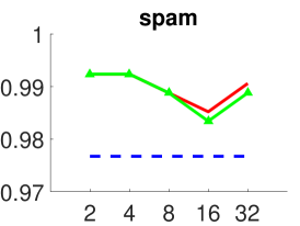
(a)

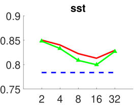
(b)

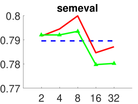
(c)

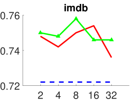
(d)

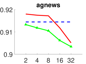
(e)

(f)

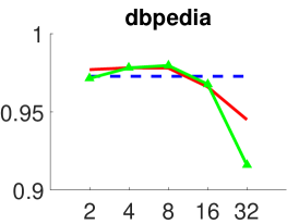
(g)

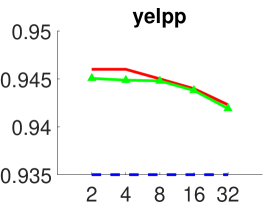
(h)

(i)

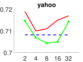
(j)

(k)

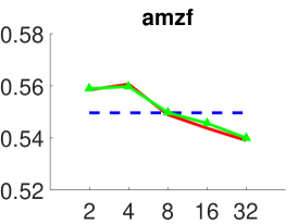
(l)

Figure 4: Comparison of testing accuracy (%) of fastText (dotted blue), TMPCA+Dense (red solid), and PCA+Dense (green head dotted), where the horizontal axis is the input length $N$.

Table 8: The relative mutual information ratio (TMPCA versus Mean).

	$N=2$	$N=4$	$N=8$	$N=16$	$N=32$
spam	1.32e+02	7.48e+05	2.60e+12	5.05e+14	9.93e+12
sst	8.48e+03	1.22e+10	1.28e+15	8.89e+15	9.17e+13
semeval	5.52e+03	1.13e+09	3.30e+14	4.78e+15	1.67e+13
imdb	1.34e+04	3.49e+09	1.89e+14	8.73e+14	1.05e+13
agnews	4.10e+05	5.30e+10	7.09e+11	3.56e+12	6.11e+12
sogou	5.53e+08	1.37e+13	6.74e+13	5.40e+13	4.21e+13
dbpedia	20.2	111	227	814	306
yelpp	8.42e+04	2.79e+11	3.85e+15	5.65e+16	1.46e+16
yelpf	2.29e+07	1.90e+11	5.92e+12	5.42e+12	1.58e+12
yahoo	6.7	9.1	9.9	5.8	1.5
amzp	7.34e+05	4.48e+11	1.24e+16	1.15e+18	2.75e+18
amzf	3.09e+06	1.47e+10	3.38e+11	1.48e+12	2.37e+12

Table 9: The relative mutual information ratio (PCA versus TMPCA).

	$N=4$	$N=8$	$N=16$	$N=32$
spam	1.04	1.00	1.00	1.49
sst	1.00	1.00	1.00	1.36
semeval	0.99	1.00	1.00	1.09
imdb	1.02	1.00	1.00	1.29
agnews	1.00	1.01	1.40	2.92
sogou	1.00	1.20	1.66	5.17
dbpedia	1.16	1.63	1.65	1.75
yelpp	1.00	1.00	1.00	1.13
yelpf	1.00	1.01	1.01	1.10
yahoo	1.01	1.30	1.94	8.78
amzp	1.00	1.00	1.00	1.10
amzf	1.00	1.00	1.03	1.41

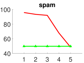
(a)

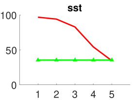
(b)

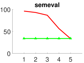
(c)

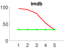
(d)

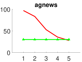
(e)

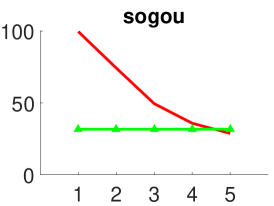
(f)

(g)

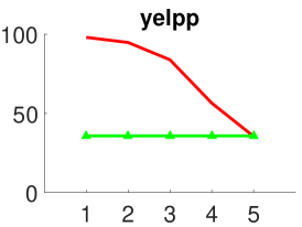
(h)

(i)

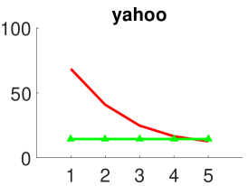
(j)

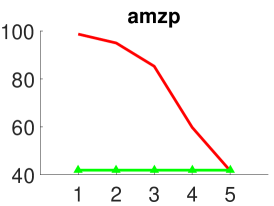
(k)

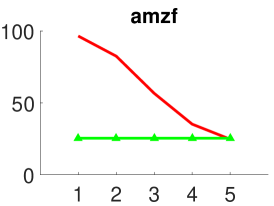
(l)

Figure 5: The energy of TMPCA (red solid) and PCA (green head dotted) coefficients is expressed as percentages of the energy of input sequences of length $N=32$, where the horizontal axis indicates the TMPCA stage number while PCA has only one stage.

5 Conclusion

An efficient language data dimension reduction technique, called the TMPCA method, was proposed for TC problems in this work. TMPCA is a multi-stage PCA in special form, and it can be described by a transform matrix with orthonormal rows. It can retain the input information by maximizing the mutual information between its input and output, which is beneficial to TC problems. It was shown by experimental results that a dense network trained on the TMPCA preprocessed data outperforms state-of-the-art fastText, char-CNN and LSTM in quite a few TC datasets. Furthermore, the number of parameters used by TMPCA is an order of magnitude smaller than other NN-based models. Typically, TMPCA takes less than one second training time on a large-scale dataset that has millions of samples. To conclude, TMPCA is a powerful dimension reduction pre-processing tool for text classification for its low computational complexity, low storage requirement for model parameters and high information preserving capability.

6 Declarations of interest

Declarations of interest: none

7 Acknowledgements

This research did not receive any specific grant from funding agencies in the public, commercial, or not-for-profit sectors.

Appendix A: Detailed Derivation of TMPCA System Function

We use the same notations in Sec. 3. For stage $s>1$, we have:

$$z^{s}_{j}=U^{s}\begin{bmatrix}z^{s-1}_{2j-1}\\ z^{s-1}_{2j}\end{bmatrix}=U^{s}_{1}z^{s-1}_{2j-1}+U^{s}_{2}z^{s-1}_{2j},$$ (18)

where $j=1,\cdots,\frac{N}{2^{s}}$. When $s=1$, we have

$$z^{1}_{j}=U^{1}_{1}w_{2j-1}+U^{1}_{2}w_{2j}$$ (19)

From Eqs. (18) and (19), we get

$$Y =z^{L}_{1}=\sum^{N}_{j=1}\Big{(}\prod^{L}_{s=1}U^{s}_{f_{j,s}}\Big{)}w_{j},$$ (20)

$$f_{j,s} =b_{L}(j-1)_{s}+1,$$ (21)

where $b_{L}(x)_{s}$ is the $s$th digit of the binarization of $x$ of length $L$. Eq. (20) can be further simplified to Eq. (6). For example, if $N=8$, we obtain

$$Y= U^{3}_{1}U^{2}_{1}U^{1}_{1}w_{1}+U^{3}_{1}U^{2}_{1}U^{1}_{2}w_{2}+U^{3}_{1}U^{2}_{2}U^{1}_{1}w_{3}+U^{3}_{1}U^{2}_{2}U^{1}_{2}w_{4}+$$

$$U^{3}_{2}U^{2}_{1}U^{1}_{1}w_{5}+U^{3}_{2}U^{2}_{1}U^{1}_{2}w_{6}+U^{3}_{2}U^{2}_{2}U^{1}_{1}w_{7}+U^{3}_{2}U^{2}_{2}U^{1}_{2}w_{8}.$$ (22)

The superscripts of $U^{s}_{j}$ are arranged in the stage order of $L,L-1,...,1$. The subscripts are shown in Table 10. This is the reason that binarization is required to express the subscripts in Eqs. (6) and (20).

Table 10: Subscripts of $U^{s}_{j}$

$w_{1}$	$w_{2}$	$w_{3}$	$w_{4}$	$w_{5}$	$w_{6}$	$w_{7}$	$w_{8}$
1,1,1	1,1,2	1,2,1	1,2,2	2,1,1	2,1,2	2,2,1	2,2,2

References

- Almeida \BOthers. (\APACyear2011) \APACinsertmetastardata_SMS_SPAM[dataset] {APACrefauthors}Almeida, T\BPBIA., Hidalgo, J\BPBIM\BPBIG.\BCBL \BBA Yamakami, J\BPBIM. \APACrefYearMonthDay2011. \APACrefbtitleContributions to the Study of SMS Spam Filtering: New Collection and Results. Contributions to the study of sms spam filtering: New collection and results. \APAChowpublishedhttps://archive.ics.uci.edu/ml/datasets/sms+spam+collection. \PrintBackRefs\CurrentBib
- Araque \BOthers. (\APACyear2017) \APACinsertmetastarsentiment_deep{APACrefauthors}Araque, O., Corcuera-Platas, I., Sánchez-Rada, J\BPBIF.\BCBL \BBA Iglesias, C\BPBIA. \APACrefYearMonthDay2017Jul. \BBOQ\APACrefatitleEnhancing deep learning sentiment analysis with ensemble techniques in social applications Enhancing deep learning sentiment analysis with ensemble techniques in social applications.\BBCQ \APACjournalVolNumPagesExpert Systems with Applications77236–246. \PrintBackRefs\CurrentBib
- Bengio \BOthers. (\APACyear2003) \APACinsertmetastarSparsity{APACrefauthors}Bengio, Y., Ducharme, R., Vincent, P.\BCBL \BBA Jauvin, C. \APACrefYearMonthDay2003Feb. \BBOQ\APACrefatitleA Neural Probabilistic Language Model A neural probabilistic language model.\BBCQ \APACjournalVolNumPagesJournal of Machine Learning Research321137–1155. \PrintBackRefs\CurrentBib
- Bennasar \BOthers. (\APACyear2015) \APACinsertmetastarJMIM{APACrefauthors}Bennasar, M., Hicks, Y.\BCBL \BBA Setchi, R. \APACrefYearMonthDay2015. \BBOQ\APACrefatitleFeature selection using joint mutual information maximisation Feature selection using joint mutual information maximisation.\BBCQ \APACjournalVolNumPagesExpert Systems with Applications42228520–8532. \PrintBackRefs\CurrentBib
- Bo \BBA Lee (\APACyear2005) \APACinsertmetastardata_IMDB[dataset] {APACrefauthors}Bo, P.\BCBT \BBA Lee, L. \APACrefYearMonthDay2005. \APACrefbtitlesentence polarity dataset. sentence polarity dataset. \APAChowpublishedhttp://www.cs.cornell.edu/people/pabo/movie-review-data/. \PrintBackRefs\CurrentBib
- K. Chen \BOthers. (\APACyear2016) \APACinsertmetastarTFIGM_TC{APACrefauthors}Chen, K., Zhang, Z., Long, J.\BCBL \BBA Zhang, H. \APACrefYearMonthDay2016Dec. \BBOQ\APACrefatitleTurning from TF-IDF to TF-IGM for term weighting in text classification Turning from tf-idf to tf-igm for term weighting in text classification.\BBCQ \APACjournalVolNumPagesExpert Systems with Applications66245–260. \PrintBackRefs\CurrentBib
- T. Chen \BOthers. (\APACyear2017) \APACinsertmetastarsentiment_NN{APACrefauthors}Chen, T., Xu, R., He, Y.\BCBL \BBA Wang, X. \APACrefYearMonthDay2017Apr. \BBOQ\APACrefatitleImproving sentiment analysis via sentence type classification using BiLSTM-CRF and CNN Improving sentiment analysis via sentence type classification using bilstm-crf and cnn.\BBCQ \APACjournalVolNumPagesExpert Systems with Applications72221–230. \PrintBackRefs\CurrentBib
- Cho \BOthers. (\APACyear2014) \APACinsertmetastarGRU{APACrefauthors}Cho, K., Merrienboer, B\BPBIv., Gulcehre, C., Bahdanau, D., Bougares, F., Schwenk, H.\BCBL \BBA Bengio, Y. \APACrefYearMonthDay2014. \BBOQ\APACrefatitleLearning Phrase Representations Using RNN Encoder-Decoder for Statistical Machine Translation Learning phrase representations using rnn encoder-decoder for statistical machine translation.\BBCQ \BIn \APACrefbtitleProceedings of the 2014 Conference on Empirical Methods in Natural Language Processing Proceedings of the 2014 conference on empirical methods in natural language processing (\BPGS 1724–1734). \APACaddressPublisherDoha, QatarAssociation for Computational Linguistics. \PrintBackRefs\CurrentBib
- Deerwester \BOthers. (\APACyear1990) \APACinsertmetastarLSA{APACrefauthors}Deerwester, S., Dumais, T\BPBIS., Furnas, W\BPBIG., Landauer, K\BPBIT.\BCBL \BBA Harshman, R. \APACrefYearMonthDay1990. \BBOQ\APACrefatitleIndexing by latent semantic analysis Indexing by latent semantic analysis.\BBCQ \APACjournalVolNumPagesJournal of the American society for information science416391–407. \PrintBackRefs\CurrentBib
- Elman (\APACyear1990) \APACinsertmetastarTime{APACrefauthors}Elman, J. \APACrefYearMonthDay1990. \BBOQ\APACrefatitleFinding Structure in Time Finding structure in time.\BBCQ \APACjournalVolNumPagesCognitive Science142179-211. \PrintBackRefs\CurrentBib
- Friedman \BOthers. (\APACyear1997) \APACinsertmetastarNB{APACrefauthors}Friedman, N., Dan, G.\BCBL \BBA Moises, G. \APACrefYearMonthDay1997. \BBOQ\APACrefatitleBayesian network classifiers Bayesian network classifiers.\BBCQ \APACjournalVolNumPagesMachine learning292-3131–163. \PrintBackRefs\CurrentBib
- Ghiassi \BOthers. (\APACyear2013) \APACinsertmetastarTwitter_ngram_ANN{APACrefauthors}Ghiassi, M., Skinner, J.\BCBL \BBA Zimbra, D. \APACrefYearMonthDay2013. \BBOQ\APACrefatitleTwitter brand sentiment analysis: A hybrid system using n-gram analysis and dynamic artificial neural network Twitter brand sentiment analysis: A hybrid system using n-gram analysis and dynamic artificial neural network.\BBCQ \APACjournalVolNumPagesExpert Systems with Applications40166266–6282. \PrintBackRefs\CurrentBib
- Hochreiter \BBA Schmidhuber (\APACyear1997) \APACinsertmetastarLSTM{APACrefauthors}Hochreiter, S.\BCBT \BBA Schmidhuber, J. \APACrefYearMonthDay1997. \BBOQ\APACrefatitleLong Short-term Memory Long short-term memory.\BBCQ \APACjournalVolNumPagesNeural Computation981735–1780. \PrintBackRefs\CurrentBib
- Joachims (\APACyear1998) \APACinsertmetastarTC_SVM{APACrefauthors}Joachims, T. \APACrefYearMonthDay1998Apr. \BBOQ\APACrefatitleText categorization with support vector machines: Learning with many relevant features Text categorization with support vector machines: Learning with many relevant features.\BBCQ \BIn \APACrefbtitleProceedings of the 10th European Conference on machine learning Proceedings of the 10th european conference on machine learning (\BPGS 137–142). \APACaddressPublisherBerlin, GermanySpringer. \PrintBackRefs\CurrentBib
- Joulin \BOthers. (\APACyear2017) \APACinsertmetastarfastText{APACrefauthors}Joulin, A., Grave, E., Bojanowski, P.\BCBL \BBA Mikolov, T. \APACrefYearMonthDay2017. \BBOQ\APACrefatitleBag of tricks for efficient text classification Bag of tricks for efficient text classification.\BBCQ \BIn \APACrefbtitleProceedings of the 15th Conference of European Chapter of the Association for Computational Linguistics Proceedings of the 15th conference of european chapter of the association for computational linguistics (\BPGS 427–431). \APACaddressPublisherValencia, SpainAssociation for Computational Linguistics. \PrintBackRefs\CurrentBib
- Kingma \BBA Ba (\APACyear2015) \APACinsertmetastarADAM{APACrefauthors}Kingma, D\BPBIP.\BCBT \BBA Ba, J. \APACrefYearMonthDay2015. \BBOQ\APACrefatitleAdam: a method for stochastic optimization Adam: a method for stochastic optimization.\BBCQ \BIn \APACrefbtitleProceedings of the 3th International Conference on Learning Representations. Proceedings of the 3th international conference on learning representations. \APACaddressPublisherSan Diego, USAICLR. \PrintBackRefs\CurrentBib
- Kontopoulos \BOthers. (\APACyear2013) \APACinsertmetastarTwitter_ontology{APACrefauthors}Kontopoulos, E., Berberidis, C., Dergiades, T.\BCBL \BBA Bassiliades, N. \APACrefYearMonthDay2013. \BBOQ\APACrefatitleOntology-based sentiment analysis of twitter posts Ontology-based sentiment analysis of twitter posts.\BBCQ \APACjournalVolNumPagesExpert Systems with Applications40104065–4074. \PrintBackRefs\CurrentBib
- Lai \BOthers. (\APACyear2016) \APACinsertmetastarGoodEmbedding{APACrefauthors}Lai, S., Liu, K., Xu, L.\BCBL \BBA Zhao, J. \APACrefYearMonthDay2016. \BBOQ\APACrefatitleHow to generate a good word embedding How to generate a good word embedding.\BBCQ \APACjournalVolNumPagesIEEE Intelligent Systems3165–14. \PrintBackRefs\CurrentBib
- Linsker (\APACyear1988) \APACinsertmetastarPCA_MI{APACrefauthors}Linsker, R. \APACrefYearMonthDay1988Mar. \BBOQ\APACrefatitleSelf-organization in a perceptual network Self-organization in a perceptual network.\BBCQ \APACjournalVolNumPagesComputer213105–117. \PrintBackRefs\CurrentBib
- Mikolov \BOthers. (\APACyear2013) \APACinsertmetastarWord2vec{APACrefauthors}Mikolov, T., Sutskever, I., Chen, K., Corrado, G.\BCBL \BBA Dean, J. \APACrefYearMonthDay2013. \BBOQ\APACrefatitleDistributed Representations of Words and Phrases and their Compositionality Distributed representations of words and phrases and their compositionality.\BBCQ \BIn \APACrefbtitleProceedings of the 27th International Conference on Advances in Neural Information Processing Systems Proceedings of the 27th international conference on advances in neural information processing systems (\BPGS 3111–3119). \APACaddressPublisherLake Tahoe, USACurran Associates. \PrintBackRefs\CurrentBib
- Mirńczuk \BBA Protasiewicz (\APACyear2018) \APACinsertmetastaroverview_TC{APACrefauthors}Mirńczuk, M\BPBIM.\BCBT \BBA Protasiewicz, J. \APACrefYearMonthDay2018Sep. \BBOQ\APACrefatitleA Recent Overview of the State-of-the-Art Elements of Text Classification A recent overview of the state-of-the-art elements of text classification.\BBCQ \APACjournalVolNumPagesExpert Systems with Applications10636–54. \PrintBackRefs\CurrentBib
- Moraes \BOthers. (\APACyear2013) \APACinsertmetastarSVM_ANN{APACrefauthors}Moraes, R., Valiati, F., JoāO\BCBL \BBA Neto, W\BPBIP\BPBIG. \APACrefYearMonthDay2013. \BBOQ\APACrefatitleDocument-level sentiment classification: An empirical comparison between SVM and ANN Document-level sentiment classification: An empirical comparison between svm and ann.\BBCQ \APACjournalVolNumPagesExpert Systems with Applications402621–633. \PrintBackRefs\CurrentBib
- Salton \BBA Buckley (\APACyear1988) \APACinsertmetastarIDF{APACrefauthors}Salton, G.\BCBT \BBA Buckley, C. \APACrefYearMonthDay1988Jan. \BBOQ\APACrefatitleTerm-weighting approaches in automatic text retrieval Term-weighting approaches in automatic text retrieval.\BBCQ \APACjournalVolNumPagesInformation processing & management245513–523. \PrintBackRefs\CurrentBib
- Socher \BOthers. (\APACyear2013) \APACinsertmetastardata_SST[dataset] {APACrefauthors}Socher, R., Perelygin, A., Wu, J., Chuang, J., Manning, C., Ng, A.\BCBL \BBA Potts, C. \APACrefYearMonthDay2013. \APACrefbtitleRecursive Deep Models for Semantic Compositionality Over a Sentiment Treebank. Recursive deep models for semantic compositionality over a sentiment treebank. \APAChowpublishedhttps://nlp.stanford.edu/sentiment/. \PrintBackRefs\CurrentBib
- Stanford (\APACyear2018) \APACinsertmetastarSST_NLP_tool{APACrefauthors}Stanford. \APACrefYearMonthDay20181,May. \APACrefbtitleCoreNLP. Corenlp. \APAChowpublishedhttps://stanfordnlp.github.io/CoreNLP/. Accessed 26 July 2018 \PrintBackRefs\CurrentBib
- Su \BOthers. (\APACyearUnpublished) \APACinsertmetastarDBRNN_ELSTM{APACrefauthors}Su, Y., Huang, Y.\BCBL \BBA Kuo, C\BHBIC\BPBIJ. \APACrefYearMonthDayUnpublished. \BBOQ\APACrefatitleOn Extended Long Short-term Memory and Dependent Bidirectional Recurrent Neural Network On extended long short-term memory and dependent bidirectional recurrent neural network.\BBCQ \APACjournalVolNumPagesarXiv:1803.01686. \PrintBackRefs\CurrentBib
- Su \BOthers. (\APACyear\BIP) \APACinsertmetastarTMPCA_ICPR{APACrefauthors}Su, Y., Huang, Y.\BCBL \BBA Kuo, J\BPBIC\BHBIC. \APACrefYearMonthDay\BIP. \BBOQ\APACrefatitleEfficient text classification using tree-structured multi-linear principal component analysis Efficient text classification using tree-structured multi-linear principal component analysis.\BBCQ \BIn \APACrefbtitleProceedings of the 24th International conference on Pattern recognition. Proceedings of the 24th international conference on pattern recognition. \APACaddressPublisherBeijing, ChinaIEEE. \PrintBackRefs\CurrentBib
- Uysal (\APACyear2016) \APACinsertmetastarfeature_TC{APACrefauthors}Uysal, A\BPBIK. \APACrefYearMonthDay2016Jan. \BBOQ\APACrefatitleAn improved global feature selection scheme for text classification An improved global feature selection scheme for text classification.\BBCQ \APACjournalVolNumPagesExpert Systems with Applications4382–92. \PrintBackRefs\CurrentBib
- Wei \BOthers. (\APACyear2015) \APACinsertmetastarwordnet_chains{APACrefauthors}Wei, T., Lu, Y., Chang, H., Zhou, Q.\BCBL \BBA Bao, X. \APACrefYearMonthDay2015. \BBOQ\APACrefatitleA semantic approach for text clustering using WordNet and lexical chains A semantic approach for text clustering using wordnet and lexical chains.\BBCQ \APACjournalVolNumPagesExpert Systems with Applications4242264–2275. \PrintBackRefs\CurrentBib
- Wilson \BOthers. (\APACyear2013) \APACinsertmetastardata_SEMEVAL[dataset] {APACrefauthors}Wilson, T., Kozareva, Z., Nakov, P., Rosenthal, S., Stoyanov, V.\BCBL \BBA Ritter, A. \APACrefYearMonthDay2013. \APACrefbtitleInternational Workshop on Semantic Evaluation 2013: Sentiment Analysis in Twitter. International workshop on semantic evaluation 2013: Sentiment analysis in twitter. \APAChowpublishedhttps://www.cs.york.ac.uk/semeval-2013/task2.html. \PrintBackRefs\CurrentBib
- Yang \BBA Pedersen (\APACyear1997) \APACinsertmetastarTC_COMP{APACrefauthors}Yang, Y.\BCBT \BBA Pedersen, J. \APACrefYearMonthDay1997Jul. \BBOQ\APACrefatitleA comparative study on feature selection in text categorization A comparative study on feature selection in text categorization.\BBCQ \BIn \APACrefbtitleProceedings of the 14th International Conference on Machine Learning Proceedings of the 14th international conference on machine learning (\BPGS 412–420). \APACaddressPublisherNashville, USAMorgan Kaufmann. \PrintBackRefs\CurrentBib
- Ye \BOthers. (\APACyear2009) \APACinsertmetastarsentiment_travel{APACrefauthors}Ye, Q., Zhang, Z.\BCBL \BBA Law, R. \APACrefYearMonthDay2009. \BBOQ\APACrefatitleSentiment classification of online reviews to travel destinations by supervised machine learning approaches Sentiment classification of online reviews to travel destinations by supervised machine learning approaches.\BBCQ \APACjournalVolNumPagesExpert Systems with Applications3636527–6535. \PrintBackRefs\CurrentBib
- Zhang \BOthers. (\APACyear2015) \APACinsertmetastarConv_text{APACrefauthors}Zhang, X., Junbo, Z.\BCBL \BBA LeCun, Y. \APACrefYearMonthDay2015. \BBOQ\APACrefatitleCharacter-level convolutional networks for text classification Character-level convolutional networks for text classification.\BBCQ \BIn \APACrefbtitleProceedings of the 29th International Conference on Advances in Neural Information Processing Systems Proceedings of the 29th international conference on advances in neural information processing systems (\BPGS 649–657). \APACaddressPublisherMontréal, CanadaCurran Associates. \PrintBackRefs\CurrentBib
- Zhang \BBA Zhao (\APACyear2005) \APACinsertmetastardata_convtext[dataset] {APACrefauthors}Zhang, X.\BCBT \BBA Zhao, J. \APACrefYearMonthDay2005. \APACrefbtitleCharacter-level convolutional networks for text classification. Character-level convolutional networks for text classification. \APAChowpublishedhttp://goo.gl/JyCnZq. \PrintBackRefs\CurrentBib