Choreographies in the $n$-vortex problem

Abstract

We consider the equations of motion of $n$ vortices of equal circulation in the plane, in a disk and on a sphere. The vortices form a polygonal equilibrium in a rotating frame of reference. We use numerical continuation in a boundary value setting to determine the Lyapunov families of periodic orbits that arise from the polygonal relative equilibrium. When the frequency of a Lyapunov orbit and the frequency of the rotating frame have a rational relationship then the orbit is also periodic in the inertial frame. A dense set of Lyapunov orbits, with frequencies satisfying a diophantine equation, corresponds to choreographies of the $n$ vortices. We include numerical results for all cases, for various values of $n$, and we provide key details on the computational approach.

1 Introduction

A vortex point in an inviscid and incompressible two-dimensional fluid corresponds to a singular vorticity concentrated at a point with constant circulation, by using the Dirac delta function for the vorticity in the Euler equation. This vorticity induces a singular velocity field in the azimuthal component around the vortex point. A mathematical model for the interaction of such vortex points in the plane was derived by Helmholtz (1858) and Kirchhoff (1876). In bounded domains the equations for $n$ point vortices are derived using the Kirchhoff-Routh functions; see [25]. The first reference to the model of vortices on a sphere can be found in [18]. Recent applications of the point vortices model include Bose-Einstein condensates and semiconductors; see [5] and references therein. A relatively recent exposition of topics related to the $n$-vortex problem can be found in [30], and the references therein.

The study of equal point vortices located at the vertices of a polygon, which rotates around its center, originates in the work of Lord Kelvin (1878) and Thomson (1883). They determined the linear stability properties of this configuration in the plane. The linear stability of the polygonal relative equilibrium for the case of a disk was studied much later [22]. The nonlinear stability properties of the polygon in the plane were determined in [9], and for the case of the sphere in [8]. When the stability of the $n$-polygon of vortices with a central vortex changes, then there is a bifurcation of relative equilibria consisting of nested polygons in the plane [20], and on the sphere [24].

A choreography of the $n$-vortex problem is a solution where the $n$ vortices follow the same path. The principal aim of our article is to determine such solutions in a systematic fashion, by making use of robust boundary value continuation techniques in the presence of symmetries. The term choreography was adopted for the case of the $n$-body problem of celestial mechanics after the work of Simó [31]. The first non-circular choreography was discovered numerically for $3$ bodies in [28], and its existence was verified analytically in [14], using the direct method of calculus of variations. The results in [14] mark the beginning of the development of variational methods for this purpose, where the existence of choreographies is associated with the problem of finding critical points of the classical action of Newton’s equations of motion. However, in the case of the $n$-vortex problem it is more difficult to establish the existence of choreographies using the direct method of calculus of variations. The reason is that the action is strongly indefinite and integrable at orbits with collisions, since $\ln r$ is integrable at $r=0$.

Vortex choreographies can be constructed explicitly for $3$ vortices in the plane, using the fact that the system is integrable in that case. Similarly, choreographies for $4$ vortices in the plane have been found in [6] and on the sphere in [7], using the fact that the system can be reduced to a system with few degrees of freedom. While the $3$-vortex problem in the plane is integrable, the $n$-vortex problem for $n\geq 4$ is only integrable in special cases [3]. The absence of integrals of motion makes it difficult to find explicit choreographies for $n\geq 4$. For the case of a disk, even the $3$-vortex problem is not integrable. Surprisingly, choreographies have been constructed recently for $n$-vortices in general bounded domains, using blow-up techniques. They are located close to a stagnation point of a vortex in the domain [4] and close to the boundary of the domain [15].

Choreographies for the $n$-body problem exist along Lyapunov families that arise from the $n$-polygon of bodies in a rotating frame [10, 13]. Related results on choreographies in the discrete nonlinear Schrödinger equations can be found in [11]. These results depend only on the symmetries of the equations, and can be extended to the case of the $n$-vortex problem in radially symmetric domains. The global existence of Lyapunov families that arise from the $n$-polygon of vortices is established in the plane in [21], and on the sphere in [19]. In our current paper we determine choreographies along Lyapunov families of the $n$-vortex problem in the plane, in a disk, and on a sphere. The families emanate from the polygonal equilibrium of the vortices, with starting frequencies $\nu_{k}$ that are equal to the normal modes of oscillation of the equilibrium, and they constitute continuous families in the space of renormalized periodic functions. The global property means that the Sobolev norm or the period of the orbits along the family tends to infinity, or that the family ends in a collision or at another equilibrium.

Specifically, let $\omega$ be the frequency of rotation of the polygonal configuration in the plane, in a disk, or on a sphere, and let $\nu$ be the frequency of the Lyapunov orbit in the rotating frame. A solution of the $n$-vortex problem in a radially symmetric domain is given by $q_{j}(t)=e^{i\omega t}x_{j}(\nu t)$, where $x_{j}$ is a $2\pi$-periodic renormalized Lyapunov orbit satisfying the symmetries

$$x_{j}(t)=e^{ij\zeta}x_{n}(t+jk\zeta),\qquad\zeta=2\pi/n~{},$$ (1)

for some $k$, with $1\leq k\leq n$. A Lyapunov orbit is $\ell:m$ resonant when $\ell$ and $m$ are relatively prime such that

$$\frac{\omega}{\nu}=\frac{\ell}{m}~{},\qquad k\ell-m\in n\mathbb{Z}~{}.$$

These conditions on the frequency are satisfied for a dense set of parameter values. An $\ell:m$ resonant Lyapunov orbit is a choreography in the inertial frame and each of the integers $k$, $\ell$, and $m$ is of distinct significance for the properties of the choreographies: the choreography has winding number $\ell$ around a center, is symmetric with respect to rotations by $2\pi/m$, and the $n$ vortices form groups of $d$-polygons, where $d$ is the greatest common divisor of $k$ and $n$. For the numerical determination of the choreographies we use boundary value continuation methods, as implemented in the most recent version [16] of the AUTO software [17].

The $n$-vortex problem is not homogeneous in the case of a disk and in the case of a sphere. In these cases we can determine continuous families of choreographies that correspond to $\ell:m$-resonant Lyapunov orbits, and that are not related by a homogeneous scaling. This statement does not hold for the case of vortices in the plane. We also consider partial choreographies, in which an additional vortex of variable circulation is located at the center of the polygon. The results of our paper can be extended to the case of $n$ vortices rotating in any radially symmetric manifold. We have also observed choreographies where the vortices are arranged along a line. This phenomenon may be related to the fact that a row of evenly arranged vortices of equal vorticity is stable, according to [1] and [2].

In Section 2 we recall how a dense set of orbits along the Lyapunov families corresponds to choreographies. In Section 3 we describe in some detail the numerical continuation procedure used to determine the periodic solution families that arise from the polygonal relative equilibrium in the plane. Later sections include complementary details on the specific numerical procedure used there. In Section 4 we consider the $n$-vortex problem in a disk. Section 5 concerns the $\left(n+1\right)$-vortex problem, with $n$ vortices of unit circulation, and with an additional vortex of circulation $\mu$ at the center of the polygon. Section 6 concerns choreographies along Lyapunov families for the case of the $n$-vortex problem on a sphere, for which we present somewhat more extensive numerical results.

2 The $n$-polygon of vortices in the plane

Let $q_{j}(t)\in\mathbb{C}$ be the position of the $j$th vortex in the plane. Assume that the $n$ vortices have equal circulation for $j=1,\ldots,n$. The Hamiltonian of $n$ vortices in the plane is

$$H(q)=-\frac{1}{2}\sum_{1\leq k<j\leq n}\ln\left|q_{j}-q_{k}\right|^{2}~{},$$

and the symplectic form is $\omega=\sum_{j=1}^{n}dx_{j}\wedge dy_{j}$. Since the Hamiltonian is invariant under the group of transformations $SO(2)$, which acts as $e^{i\theta}u$, the equations also have the conserved quantity

$$G(q)=\frac{1}{2}\sum_{j=1}^{n}\left|q_{j}\right|^{2}.$$ (2)

The equations for the vortices in rotating coordinates, $q_{j}(t)=e^{i\omega t}u_{j}(t)$, are then given by

$$i\dot{u}_{j}=\omega u_{j}-\sum_{k=1~{}(k\neq j)}^{n}\frac{u_{j}-u_{k}}{\left|u_{j}-u_{k}\right|^{2}}~{},\qquad u_{j}(t)\in\mathbb{C}~{}\text{.}$$ (3)

The $n$-polygon of vortices $u_{j}=e^{ij\zeta}$, $\zeta=2\pi/n$ , for $j=1,\ldots,n$, is an equilibrium [21] when

$$\omega=\frac{n-1}{2}~{}.$$ (4)

In [21], equivariant degree theory is used to prove that the polygonal relative equilibrium has a global family of periodic solutions of the form $u_{j}(t)=x_{j}(\nu t)$, with symmetries (1), for each positive frequency

$$\nu_{k}=\left(s_{k}\left(2\omega-s_{k}\right)\right)^{1/2}~{},$$

with $k=1,\ldots,n-1$, where $s_{k}=k(n-k)/2$.

Due to rotational invariance there is always a zero frequency, $\nu_{0}=0$. Since the frequencies have $1:1$ resonances ($\nu_{k}=\nu_{n-k}$), straightforward application of the Lyapunov center theorem is not possible, except for some cases with $k=n/2$ for $n=2,4,6$, see [12]. For example, for $n=6$ we have

$$\nu_{1}=\nu_{5}=\frac{5}{2}~{},\qquad\nu_{2}=\nu_{4}=2~{},\qquad\nu_{3}=\frac{3}{2}~{}.$$

According to [10], we define a Lyapunov orbit as being $\ell:m$ resonant  if its frequency satisfies the relation

$$\frac{\omega}{\nu}=\frac{\ell}{m}~{}\text{,}$$

where $\ell$ and $m$ are relatively prime such that $k\ell-m\in n\mathbb{Z}$ . The explicit period of an $\ell:m$ resonant Lyapunov orbit is

$$T_{\ell:m}~{}=~{}\frac{2\pi}{\nu}~{}=~{}\frac{4\pi}{n-1}~{}\frac{\ell}{m}~{}.$$

Theorem 1

In the inertial frame an $\ell:m$ resonant Lyapunov orbit is a choreography, satisfying

$$q_{j}(t)=q_{n}(t+j\tilde{k}\zeta)~{}\text{,}$$

where $\tilde{k}=k-(k\ell-m)\ell^{\ast}$, with $\ell^{\ast}$ the $m$-modular inverse of $\ell$. The period of the choreography is $m~{}T_{\ell:m}$. The choreography is symmetric with respect to rotations by the angle $2\pi/m$, and it winds around a center $\ell$ times.

For a proof of this result see [10] and [19].

3 Numerical continuation of Lyapunov families

For the numerical continuation of the Lyapunov families it is necessary to take the rotational symmetries into account, i.e., to continue the Lyapunov orbits numerically, we use the augmented equations

$$\dot{u}=(-i\omega+\lambda_{1})\nabla G-(i-\lambda_{2})\nabla H~{}.$$ (5)

The solutions of Equation (5) are solutions of the original equations of motion when the unfolding parameters $\lambda_{1}$ and $\lambda_{2}$ are zero. The converse of this statement is also true, as long as the fields $\nabla G$ and $\nabla H$ are linearly independent. The unfolding parameters and the corresponding unfolding terms in Equation 5 are needed to regularize the continuation of periodic solutions in this conservative system with rotational invariance; see [29] for a general treatment of continuation of periodic orbits in conservative systems.

Below we provide key details on our computational approach, so that it can also be applied to related problems, or be implemented in other computational environments. Moreover, a directory with python scripts that make the AUTO software carry out all computations reported in this paper, as well as much more extensive computations, will be made freely available.

Due to the symmetries, most eigenvalues corresponding to the polygonal equilibrium have multiplicity $2$. In order to compute emanating families of periodic solutions, while avoiding lengthy mathematical derivations, we use a simple perturbation approach. For the stationary solutions we use the equations

$$\left(\lambda_{1}-i\right)\omega u_{j}+i\sum_{k\neq j}\kappa_{k}\frac{u_{j}-u_{k}}{\left|u_{j}-u_{k}\right|^{2}}=0,\quad j=1,\ldots n~{},$$ (6)

where $\omega=(n-1)/2$, and where $\lambda_{1}$ is an unfolding parameter that is used to regularize the initial continuation of stationary solutions. Note that for stationary solutions only one such unfolding parameter is needed, while two unfolding parameters are required for the continuation of periodic solutions. Also note that we have introduced parameters $\kappa_{j}$, $j=1,...,n$, where $\kappa_{j}=1$ for $j=1,...,n-1$, but where we treat $\kappa_{n}$ as a perturbation parameter that is allowed to take on values different from $1$. More specifically, the parameter $\kappa_{n}$ is used to perturb the circulation of the $n$-th vortex temporarily in the first few steps of the algorithm that leads to choreographies. We also add a simple constraint on the location of the $n$th vortex, which removes the rotational invariance, namely,

$$\operatorname{Im}u_{n}=0~{}.$$ (7)

Considered as real equations with real variables, Equations (6) and (7) together define a system of $2n+1$ equations. Conceptionally we may consider the $u_{j}$ and $\lambda_{1}$ as $2n+1$ real variables, and $\kappa_{n}$ as the continuation parameter, even though the continuation algorithm does not make this distinction. The perturbation procedure carries out this continuation, namely until $\kappa_{n}$ reaches a target value different from $1$, for which we have used, for example, $\kappa_{n}=1.2$. For the case $n=5$ that we consider in this section, the eigenvalues of the linearized equations for the unperturbed equations are $\pm i\nu_{1}=\pm 2i$ and $\pm i\nu_{2}=\pm i\sqrt{3}$, where each of these conjugate, purely imaginary pairs has algebraic multiplicity $2$. In addition there is a zero eigenvalue of multiplicity $2$. By contrast, the eigenvalues of the perturbed equations, with $\kappa_{n}=1.2$, are found to be $\pm 2i$, $\pm 1.99717i$, $\pm 1.74814i$, and $\pm 1.72256i$, as well as two real eigenvalues of opposite sign that are very close to zero. These four purely imaginary eigenvalues are simple, and each gives rise to a family of periodic solutions.

Each bifurcating family of periodic orbits is computed in three stages. The first stage is to follow the Lyapunov family starting from the perturbed equilibrium (with $\kappa_{n}$ close to, but different from $1$), and until the amplitude of the periodic orbit reaches a small target value. Here the “amplitude” is defined as

$$A=\sum_{j=1}^{n}\int_{0}^{1}|u_{j}(t)-u_{j}^{0}|^{2}~{}dt~{},$$ (8)

where $u_{j}^{0}$ denotes the equilibrium position of the $j$th component. Thus the amplitude is zero at the perturbed equilibrium. In the second stage this small amplitude orbit is followed keeping the amplitude fixed, while allowing $\kappa_{n}$ to vary until it returns to the value $1$. This nontrivial periodic orbit is then a solution of the unperturbed equations. In the third stage this orbit is followed, keeping $\kappa_{n}$ fixed at $1$ and allowing the amplitude to vary again, thereby generating the desired solution family of the unperturbed problem.

Each of the three stages referred to above utilizes a boundary value formulation for the continuation of periodic solutions. The differential equation is here written as

$$\dot{u}_{j}=T(\lambda_{1}-i)\omega u_{j}-T(\lambda_{2}-i)\sum_{k\neq j}\kappa_{k}\frac{u_{j}-u_{k}}{\left|u_{j}-u_{k}\right|^{2}},\quad j=1,\ldots n~{},$$ (9)

where time has been rescaled to the unit interval $[0,1]$, so that the actual period $T$ appears explicitly in the differential equations. The periodicity boundary constraints are then given by

$$u_{j}(1)-u_{j}(0)=0~{},\qquad j=1,\ldots,n~{}.$$ (10)

The boundary value formulation also contains integral constraints. One of these is the usual integral phase condition, here applied to the $n$th vortex only, namely,

$$\operatorname{Re}\int_{0}^{1}u_{n}(t)~{}\dot{\tilde{u}}_{n}(t)~{}dt=0~{},$$ (11)

where $\dot{\tilde{u}}_{n}(t)$ represents the time derivative of a reference solution, namely the preceding solution in the numerical continuation process. Another integral constraint sets the average of the imaginary part of the $n$th vortex to zero, namely,

$$\operatorname{Im}\int_{0}^{1}u_{n}(t)~{}dt=0~{}.$$ (12)

This second integral constraint removes the rotational invariance of periodic orbits. There are more general integral constraints for fixing the phase and for removing invariances. However the ones listed above are simple, and appropriate in the current context. Furthermore, one can keep track of the “amplitude” (8) of the orbits. More importantly, one can also choose to keep this amplitude fixed, by adding it as an integral constraint.

As outlined above, the determination of each bifurcating family of periodic solutions is done in three stages. In the first stage, with perturbed circulation $\kappa_{n}$, the free scalar parameters are the amplitude $A$, the period $T$, and the unfolding parameters $\lambda_{1}$ and $\lambda_{2}$. In the second stage, where the perturbation is being undone, the free parameters are the circulation of the $n$th vortex, namely, $\kappa_{n}$, the period $T$, and $\lambda_{1}$ and $\lambda_{2}$, while the amplitude $A$ remains fixed at a small, nonzero value. In the third stage, where the actual family of interest is computed, the free parameters are again those used in stage 1, namely, $A$, $T$, $\lambda_{1}$, and $\lambda_{2}$. Figure 1 shows a representation of one of the four periodic solution families that arise from the polygonal equilibrium for the case of $5$ vortices in the plane. More specifically, this family is one of the two families that arise from the complex conjugate purely imaginary eigenvalue $\pm i\sqrt{3}$, which has algebraic multiplicity $2$. Three representative periodic solutions along this family can be seen in Figure 2; each shown in the rotating frame, as well as in the inertial frame, where they correspond to choreographies.

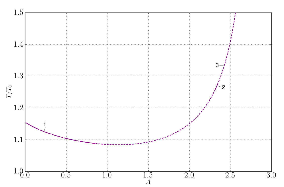
Figure 1: A representation of one of the four families of periodic solutions for the case of 5 vortices in the plane, showing the resonance ratio versus the amplitude parameter $A$. Solid curve sections correspond to stable or almost stable solutions, and dashed sections correspond to unstable solutions. The solutions labeled $1$, $2$, and $3$ correspond to the choreographies shown in Figure 2. Solutions $1$ and $2$ are stable, with resonance ratio $9:8$, and $33:26$, repectively. Solution $3$ is unstable, with resonance ratio $4:3$. Further data on these orbits can be found in Table 1.

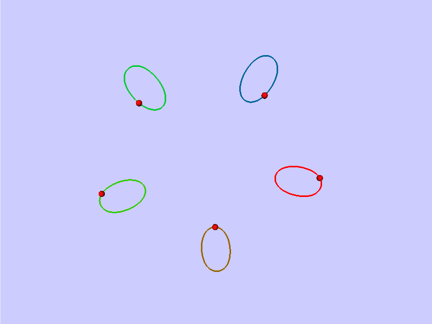
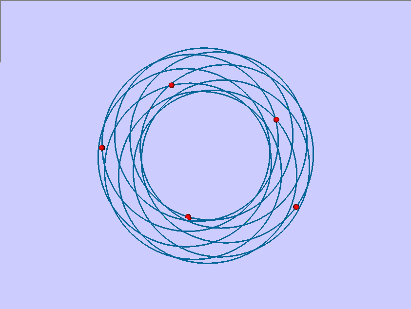
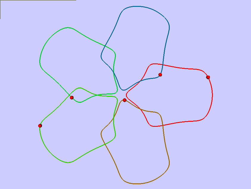
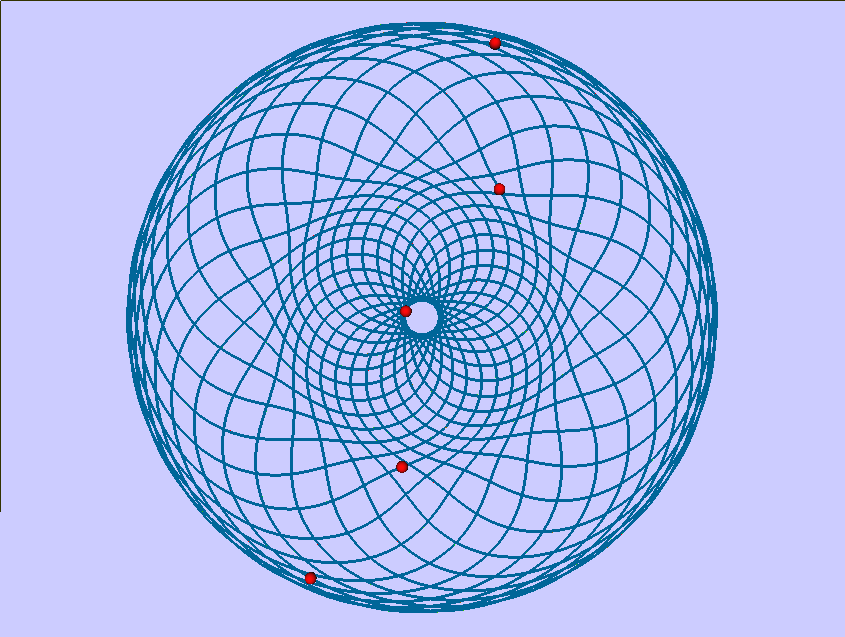
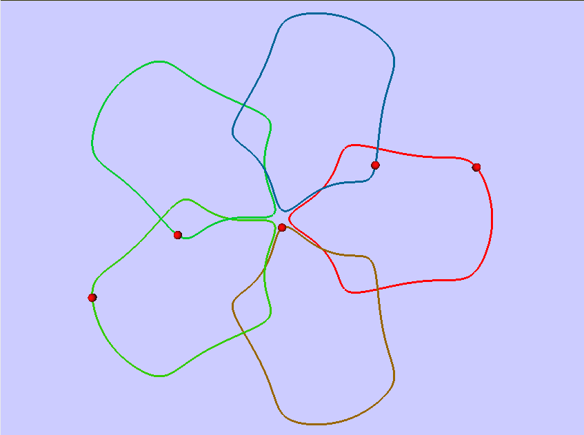
Figure 2: The case of 5 vortices in the plane, for which a bifurcation diagram is shown in Figure 1. Numerical data can be found in Table 1. The panels on the left show periodic solutions in the rotating frame. The panels on the right show the corresponding periodic solutions in the inertial frame, where they correspond to choreographies.

4 The vortex polygon in a disk

Let $B_{R}\subset\mathbb{C}$ be the disk of radius $R$, and let $q_{j}(t)\in B_{R}$ be the position of the $j$th vortex. Assume that the $n$ vortices have equal circulation for $j\in\{1,\ldots,n\}$. According to [26], the Hamiltonian of $n$ vortices in the disk $B_{R}$ is given by

$$H(q)=-\frac{1}{2}\sum_{k<j}\ln\left|q_{j}-q_{k}\right|^{2}+\frac{1}{4}\sum_{j,k=1}^{n}\ln\left|R^{2}-q_{j}\bar{q}_{k}\right|^{2}~{}.$$

The symplectic form and the conserved quantity $G(q)$ are the same as in the case of the plane. The equations of motion are given by

$$i\dot{q}_{j}=-\sum_{k\neq j}\frac{q_{j}-q_{k}}{\left|q_{j}-q_{k}\right|^{2}}+\sum_{k=1}^{n}\frac{q_{j}-\hat{q}_{k}}{\left|q_{j}-\hat{q}_{k}\right|^{2}}~{},\qquad q_{j}(t)\in B_{R}~{},$$

where the second sum represents the interaction with the boundary, with

$$\hat{q}_{k}=R^{2}/\bar{q}_{k}~{}.$$

Since $\hat{q}_{k}=e^{i\omega t}\hat{u}_{k}$, with $\hat{u}_{k}=R^{2}/\bar{u}_{k}$, the equations of the $n$ vortices in rotating coordinates, $q_{j}(t)=e^{i\omega t}u_{j}(t)$, are given by

$$i\dot{u}_{j}=\omega u_{j}-\sum_{k\neq j}\frac{u_{j}-u_{k}}{\left|u_{j}-u_{k}\right|^{2}}+\sum_{k=1}^{n}\frac{u_{j}-\hat{u}_{k}}{\left|u_{j}-\hat{u}_{k}\right|^{2}}~{},\qquad u_{j}(t)\in B_{R}~{}.$$ (13)

For a proper choice of $\omega$, there is always an equilibrium of the form $u_{j}=R_{0}e^{ij\zeta}$ with $\zeta=2\pi/n$. Without loss of generality we can assume, after a rescaling if necessary, that $R_{0}=1$. We use the radius $R$ of the disk as the problem parameter. The frequency of rotation of the polygonal equilibrium $u_{j}=e^{ij\zeta}$, with $R>1$ [22], is given by

$$\omega=\frac{n}{1-R^{-2n}}-\frac{n+1}{2}~{}.$$ (14)

The theorem in [21] can also be applied to the polygonal relative equilibrium in the disk. It implies that the polygon has a global family of periodic solutions of the form $u_{j}(t)=x_{j}(\nu t)$ with symmetries (1) for each normal mode of oscillation. These normal modes are the purely imaginary eigenvalues of the linearization, which correspond to the linearly stable eigenvalues analyzed in [22]. Theorem 1 and its numerical implementation in the plane are applicable in the disk as well, i.e., the $\ell:m$ resonant Lyapunov orbits in the disk, with period $T_{\ell:m}=2\pi\frac{\ell}{\omega m}$, correspond to choreographies in the inertial frame.

The augmented equations for the numerical determination of the families of periodic solutions for the case of a disk are given by

$$\dot{u}_{j}=T(\lambda_{1}-i)~{}\omega u_{j}+T(\lambda_{2}-i)\left(\sum_{k\neq j}\frac{u_{j}-u_{k}}{\left|u_{j}-u_{k}\right|^{2}}-\sum_{k=1}^{n}\frac{u_{j}-\hat{u}_{k}}{\left|u_{j}-\hat{u}_{k}\right|^{2}}\right)~{},$$

which include two unfolding terms, multiplied by their respective unfolding parameters $\lambda_{1}$ and $\lambda_{2}$.

For the case of vortices in a disk, the numerical determination of the families of periodic orbits that arise from the polygonal equilibrium is easier than for the case of the plane. The reason is that the purely imaginary eigenvalues are now simple, although they approach higher multiplicity when the radius parameter $R$ gets large. We also observe that for small values of $R$ there can be unstable eigenvalues. One of the several cases that we have considered in detail is that of $5$ vortices in a disk. When $R=6$ then the purely imaginary eigenvalues for the case $n=5$ are given by $\{1.99999i,~{}1.86111i,~{}1.73111i,~{}1.72371i\}$. Thus the perturbation approach used for the case of vortices in the plane is not needed now. Apart from that, the formulation of the boundary value problem for computing the families of periodic solutions is similar to that for the case of the plane. In particular, the same periodicity boundary conditions and integral constraints can be used.

The presence of a problem parameter, namely $R$, allows for additional continuation schemes; for example, where a solution quantity such as the period $T$ or the resonance ratio $T/T_{0}$ is fixed, while $R$ is free to vary. As a variation on this, we have found it useful here to implement a continuation scheme where the $n$th vortex at time zero, i.e., $u_{n}(0)$, is constrained to be located on the $x$-axis and near the origin; see, for example, the panels on the left in Figure 4. To this end we add the following two boundary conditions to the periodicity Equations (10):

$$\operatorname{Im}u_{n}(0)~{}=~{}0\quad\mbox{and}\quad\operatorname{Re}u_{n}(0)~{}-~{}r_{n}~{}=~{}0~{},$$ (15)

which also introduces a parameter $r_{n}$, which can be chosen to remain fixed or be free to vary. The condition $\operatorname{Im}u_{n}(0)=0$ replaces the integral phase condition (11), while the integral constraint (12) that inhibits rotation remains included. As a result, the parameter $r_{n}$ then corresponds to the closest approach of the $n$th vortex to the origen. By symmetry, the value of $r_{n}$ also corresponds to the closest approach to the origen of the other vortices. Furthermore, the integral constraint (8) that keeps track of the amplitude of the orbits, also remains included. Effectively, the continuation system then includes $2n+2$ real boundary constraints and $2$ real integral constraints. Since the system of differential equations corresponds to $2n$ real equations, there must be $5$ free scalar parameters to compute a 1-dimensional continuum of periodic orbits. Periodic orbits are first continued with $r_{n}$, $A$, $T$, $\lambda_{1}$, and $\lambda_{2}$ as the five free parameters, namely until $r_{n}$ reaches a desired target value. Subsequently this target orbit is continued keeping $r_{n}$ fixed, while allowing the problem parameter $R$ to vary. The five free continuation parameters in this step are therefore $R$, $A$, $T$, $\lambda_{1}$, and $\lambda_{2}$.

A representative bifurcation diagram for the case $n=5$, with $r_{n}=0.2$, is shown in Figure 3. The family that is shown there arises indirectly from the purely imaginary eigenvalue $1.72371i$ of the polygonal equilibrium. The family that emanates directly from this equilibrium is followed until it reaches the target orbit having $r_{n}=0.2$. Subsequently the target orbit is followed keeping $r_{n}$ fixed, while allowing the problem parameter $R$ to vary. Also varying in this secondary continuation is the period $T$, while the base period $T_{0}$ of the rotating frame is a direct function of $R$, namely $T_{0}=2\pi/\omega$, with $\omega=\omega(R)$ defined in Equation 14. Figure 3 provides a representation of the solution family that is generated in the secondary continuation, by showing the value of the resonance ratio $T/T_{0}$ versus the parameter $R$.

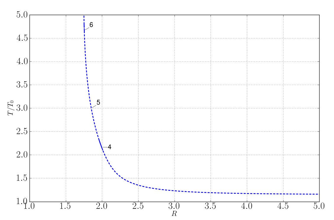
Figure 3: One of the four families of periodic solutions that bifurcate from the polygonal equilibrium for the case of 5 vortices in a disk. Solid curve sections represent stable or almost stable solutions. In particular, solutions 4 and 6 are seen to be stable, while solution 5 is unstable. The solutions labeled $4$, $5$, and $6$ correspond to choreographies, with the actual orbits shown in Figure 4. As explained in the text, all orbits along this family share the property that their closest approach to the origin is equal to $r_{n}=0.2$. Further data on the labeled solutions can be found in Table 1.

Along the solution path in Figure 3 there exists a countably infinite number of resonant orbits that correspond to choreographies in the inertial frame. Numerically we can in principle locate an unlimited number of these. Three such choreographic solutions are indicated by the labeled points in Figure 3. The resonance ratio of these solutions is $13:6$ (label 4), $3:1$ (label 5), and $14:3$ (label 6), respectively. The actual orbits of the three labeled solutions in Figure 3 are shown in Figure 4. The panels on the left in Figure 4 show these resonant orbits in the rotating frame, and the panels on the right show the corresponding orbits in the inertial frame, where they correspond to choreographies. Observe that in Figure 4 the path of the $n$th vortex, where $n=5$, is the one that is symmetric with respect to the real axis. The closest approach to the origen occurs at time $t=0$, as a result of the boundary and integral constraints described above.

Data on the solutions labeled 4, 5, and 6 in Figure 3 is given in Table 1. In particular, solutions 4 and 6 are seen to be stable, while solution 5 is unstable, as can also be inferred from Figure 3. The magnitude of the largest Floquet multiplier of the unstable solution 5 is found to be $7.39340$. The particular manner by which these solutions were obtained, as described above, represents one of various computational schemes that we have used in the quest to locate stable solutions. As illustrated in Figure 3, regions of stability along solution families can be relatively small, and therefore require a systematic approach for their determination.

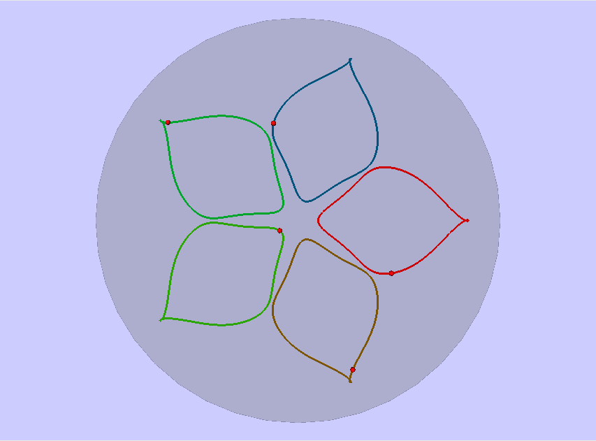
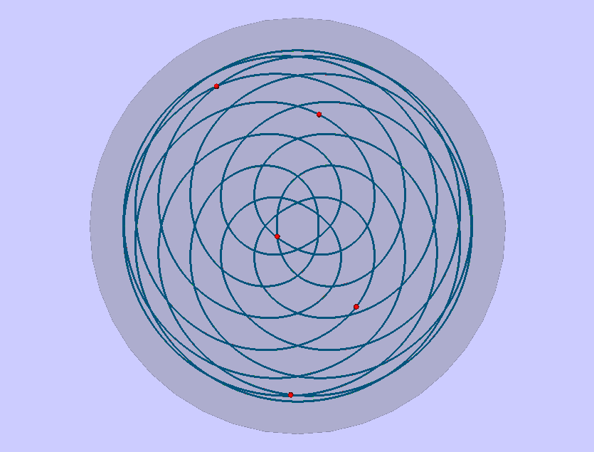
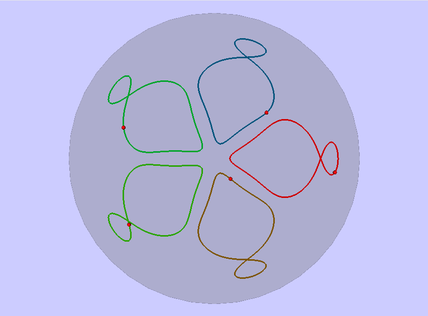
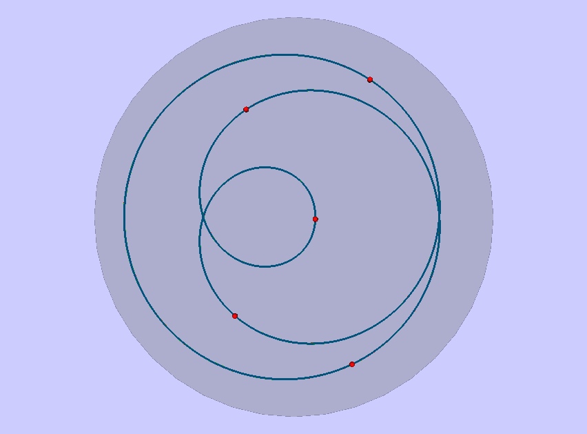
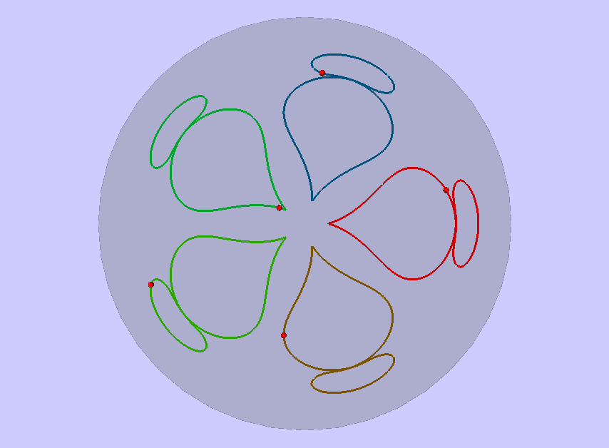
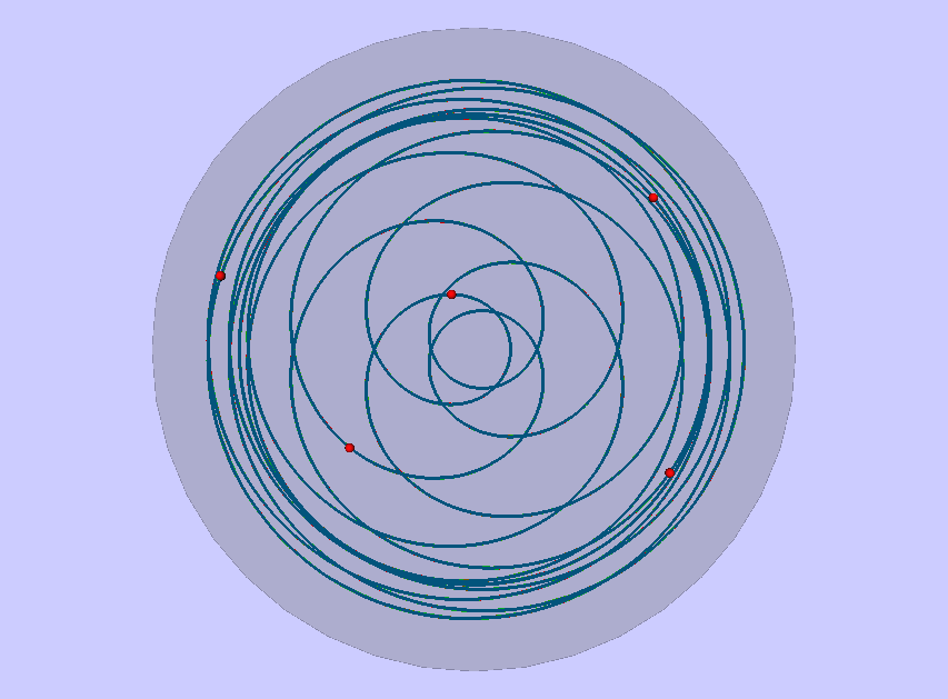
Figure 4: The case of $n$ vortices in a disk, where $n=5$, for which a bifurcation diagram is shown in Figure 3. Numerical data can be found in Table 1. The three rows of two panels correspond to the solutions labeled $4$, $5$, and $6$, respectively, in Figure 3. The panels on the left show periodic solutions in the rotating frame. Here the path of the $n$th vortex is symmetric with respect to the real axis, and its closest approach to the origen occurs at time $t=0$, as a result of the boundary and integral constraints described in the text. The panels on the right show the corresponding periodic solutions in the inertial frame, where they correspond to choreographies.

5 The vortex polygon with a center vortex

Let $q_{j}(t)\in\mathbb{C}$ be the position of the $j$th vortex in the plane, for $j=0,1,\ldots,n$. Assume the $n$ vortices with $j=1,\ldots,n$ have circulation $1$, and the vortex with $j=0$ has circulation $\mu$. The Hamiltonian is

$$H(q)=-\frac{1}{2}\sum_{1\leq k<j\leq n}\ln\left|q_{j}-q_{k}\right|^{2}-\frac{1}{2}\mu\sum_{k=1}^{n}\ln\left|q_{0}-q_{j}\right|^{2}~{},$$

with symplectic form

$$\omega=\mu\left(dx_{0}\wedge dy_{0}\right)+\sum_{j=1}^{n}dx_{j}\wedge dy_{j}~{},$$

and conserved quantity

$$G(q)=\mu\frac{1}{2}\left|q_{0}\right|^{2}+\frac{1}{2}\sum_{j=1}^{n}\left|q_{j}\right|^{2}~{}.$$

The equations of motion of the $n$ vortices in rotating coordinates, $q_{j}(t)=e^{i\omega t}u_{j}(t)$, are given by

$$i\dot{u}_{j}=\omega u_{j}-\mu\frac{u_{j}-u_{0}}{\left|u_{j}-u_{0}\right|^{2}}-\sum_{k\neq j}\frac{u_{j}-u_{k}}{\left|u_{j}-u_{k}\right|^{2}}~{},\quad j=1,\ldots,n~{},$$ (16)

$$i\dot{u}_{0}=\omega u_{0}-\sum_{k=1}^{n}\frac{u_{0}-u_{k}}{\left|u_{0}-u_{k}\right|^{2}}~{}.$$

The vortex ring with a center corresponds to the positions $u_{0}=0$, and $u_{j}=e^{ij\zeta}$, $j=1,\ldots,n$. This configuration is an equilibrium when

$$\omega=\mu+s_{1}=\mu+\frac{n-1}{2}~{}.$$ (17)

The configuration has a global family of periodic solutions of the form $u_{j}(t)=x_{j}(\nu t)$, with symmetries (1) for each positive frequency $\nu_{k}=\left(s_{k}(2\omega-s_{k})\right)^{1/2}$, where $s_{k}=k(n-k)/2$ [21]. Theorem 1, and the numerical algorithms for $n$ equal vortices, are also applicable to the current case of $n+1$ vortices. Here an $\ell:m$ resonant Lyapunov orbit has period

$$T_{\ell:m}=\frac{2\pi}{\omega}\frac{\ell}{m}~{}.$$

For these resonant orbits, $n$ vortices move in a choreographic fashion in the inertial frame, while the central vortex follows a separate closed curve.

The augmented system of equations used for numerical continuation of periodic orbits is now

$$\dot{u}_{j}=T\left(\lambda_{1}-i\right)\omega u_{j}-T\left(\lambda_{2}-i\right)\left(\mu\frac{u_{j}-u_{0}}{\left|u_{j}-u_{0}\right|^{2}}+\sum_{k\neq j}\frac{u_{j}-u_{k}}{\left|u_{j}-u_{k}\right|^{2}}\right)~{},\quad j=1,\ldots,n~{},$$ (18)

$$\dot{u}_{0}=T\left(\lambda_{1}-i\right)\omega u_{0}-T\left(\lambda_{2}-i\right)\sum_{k=1}^{n}\frac{u_{0}-u_{k}}{\left|u_{0}-u_{k}\right|^{2}}~{}.$$

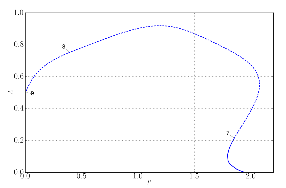
Figure 5: A continuum of choreographies of fixed resonance $T/T_{0}=11:4$, with varying circulation $\mu$ of the central vortex, for the case of 5 vortices with a 6th vortex at the center. The solutions labeled $7$, $8$, and $9$ correspond to the partial choreographies shown in Figure 6. All have the same resonance ratio, namely $11:4$, and only solution $7$ is stable.

As in Section 2 for vortices in the plane, we use a perturbation approach to deal with the purely imaginary eigenvalues of multiplicity 2, which also arise here. As in Section 4 for vortices in a disk, the presence of a problem parameter allows for additional continuation schemes. Here it was found useful to continue periodic orbits with fixed resonance ratio $T/T_{0}$, allowing the circulation $\mu$ of the center vortex to vary. To be more precise, via the perturbation approach we can compute all families that arise from the purely imaginary eigenvalues. Along these families we accurately detect selected resonances of interest; in particular those that correspond to choreographies in the inertial frame. In follow-up computations, such resonant orbits can be continued with fixed resonance ratio $T/T_{0}$, allowing the circulation parameter $\mu$ to vary. With the constraint that $T/T_{0}$ remain fixed, the standard periodicity boundary conditions, and with three integral constraints, namely the integral phase constraint applied to the $n$th vortex, the integral that sets the average $y$-coordinate of the $n$th vortex to zero, and the integral that defines the amplitude measure $A$, the full list of free continuation parameters is then given by $\mu$, $A$, $T$, $\lambda_{1}$, and $\lambda_{2}$. Note that the period $T_{0}$ of the rotating frame is taken to be a function of $\mu$, namely $T_{0}=2\pi/\omega$, with $\omega=\omega(\mu)$ defined in Equation 17. In this way we can generate a continuum of choreographies, which is useful in the search for stable ones.

Figure 5 shows such a continuum, i.e., a family of choreographies along which the resonance ratio remains constant, namely $T/T_{0}=11:4$. A selection of three choreographies along this family is indicated in Figure 5, with the actual orbits shown in Figure 6, both in the rotating and in the inertial frame. The orbit labeled 7 in Figure 5 is stable, or almost stable, with all multipliers on the unit circle in the complex plane, to at least five decimal digits accuracy. Orbit 8 is highly unstable, with two real multipliers outside the unit circle, one having magnitude $1.3205~{}10^{4}$. Orbit 9 is for a very small value of $\mu$, namely $\mu=0.005$, and is also unstable, with a complex conjugate pair of multipliers of magnitude $38.1319$. A posteriori numerical integration shows that this periodic orbit is followed for a relatively short time, after which the weak central vortex is ejected to the outside.

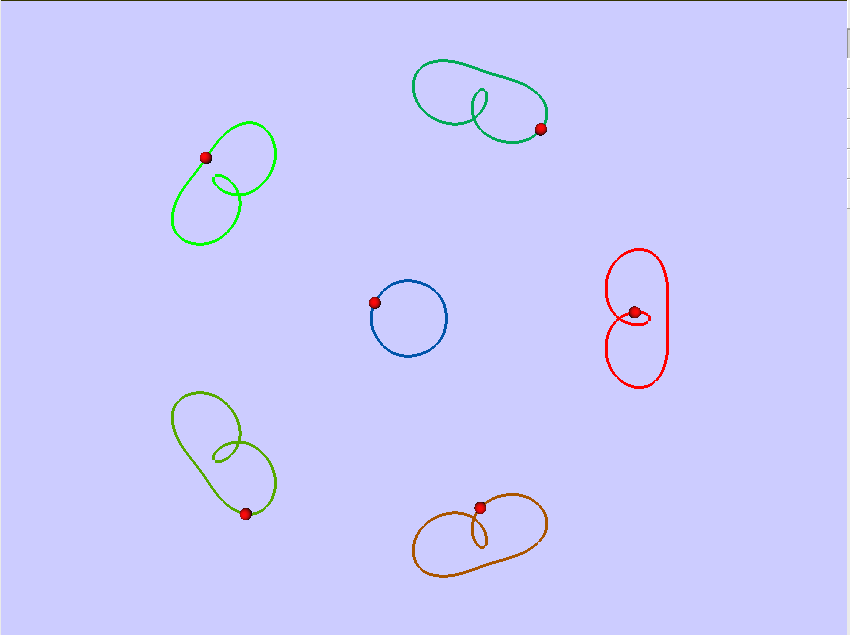
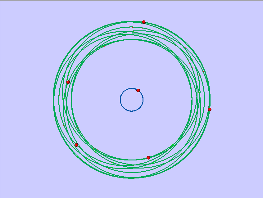
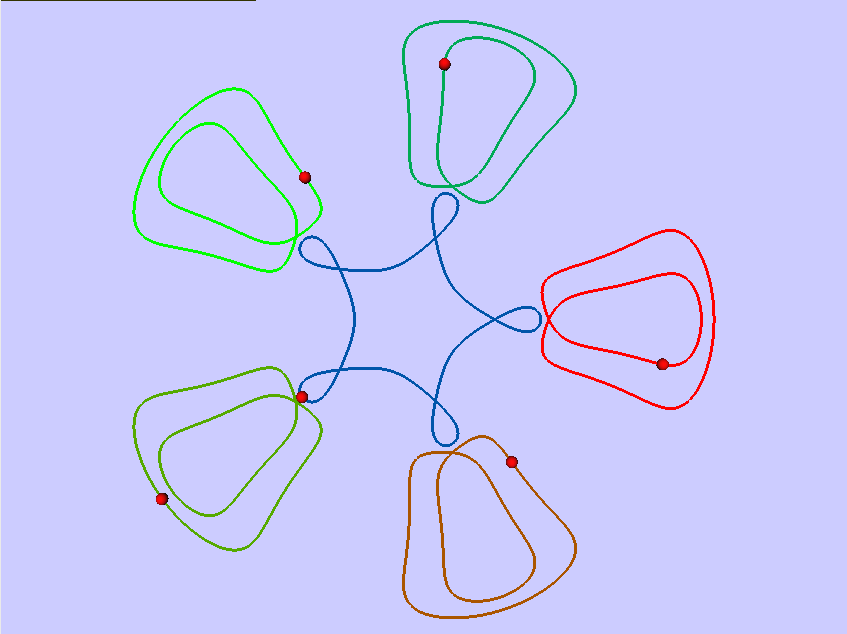
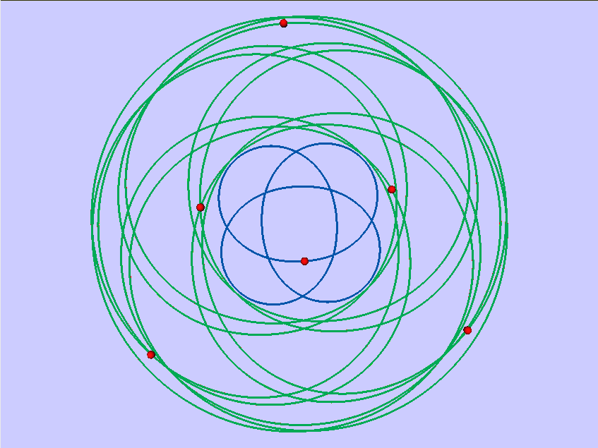
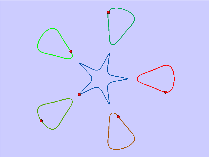
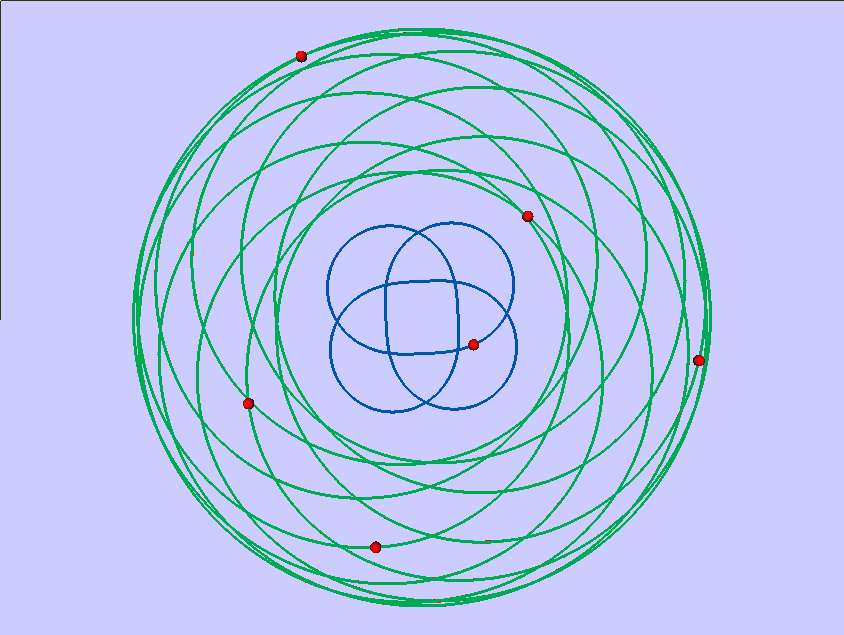
Figure 6: The case of 5 vortices of unit circulation in the plane, with a 6th vortex of variable circulation at the center. A bifurcation diagram is shown in Figure 5. Numerical data can be found in Table 1. The panels on the left show periodic solutions in the rotating frame. The panels on the right show the corresponding periodic solutions in the inertial frame, where they are seen to correspond to partial choreographies.

6 Vortices on a sphere

According to [30], the motion of $n$ vortices on the sphere $S^{2}=\{X\in\mathbb{R}^{3}:\left\|v\right\|=R\}$ is described by vectors $v_{j}(t)\in S^{2}$ that satisfy

$$\dot{v}_{j}=\frac{1}{R}\sum_{k\neq j}\frac{v_{k}\times v_{j}}{\left\|v_{j}-v_{k}\right\|^{2}}~{}.$$

Letting $v_{j}=(X_{j},Y_{j},Z_{j})$, the stereographic projection of the sphere $S^{2}$ with $R=1$ onto the complex plane is

$$q_{j}=\frac{X_{j}+iY_{j}}{1-Z_{j}}\in\mathbb{C}~{}\text{.}$$

According to [27], the Hamiltonian of the $n$ vortices on the sphere, parameterized by the stereographic projection, is given by

$$H(q)=-\frac{1}{2}\sum_{k\neq j}\ln\frac{\left|q_{j}-q_{k}\right|^{2}}{\left(1+\left|q_{j}\right|^{2}\right)\left(1+\left|q_{k}\right|^{2}\right)}~{},$$

where the simplectic form is

$$\omega=\sum_{j=1}^{n}\frac{4}{\left(1+\left|q_{j}\right|^{2}\right)^{2}}~{}dx_{j}\wedge dy_{j}~{},\qquad q_{j}=x_{j}+iy_{j}\text{~{}.}$$

Here the conserved quantity is

$$G(q)=\sum_{j=1}^{n}\frac{\left|q_{j}\right|^{2}}{1+\left|q_{j}\right|^{2}}~{}.$$ (19)

The equations of the $n$ vortices on the sphere, parameterized by the stereographic projection, are then given by

$$i\dot{q}_{j}=-\frac{1}{4}\left(1+\left|q_{j}\right|^{2}\right)^{2}\sum_{k\neq j}\left(\frac{q_{j}-q_{k}}{\left|q_{j}-q_{k}\right|^{2}}-\frac{q_{j}}{1+\left|q_{j}\right|^{2}}\right)\text{.}$$ (20)

In rotating coordinates, with $q_{j}(t)=e^{i\omega t}u_{j}(t)$, we have

$$i\dot{u}_{j}=\omega u_{j}-\frac{1}{4}\left(1+\left|u_{j}\right|^{2}\right)^{2}\sum_{k\neq j}\left(\frac{u_{j}-u_{k}}{\left|u_{j}-u_{k}\right|^{2}}-\frac{u_{j}}{1+\left|u_{j}\right|^{2}}\right)\text{.}$$ (21)

The $n$ vortices on the sphere have a polygonal equilibrium

$$u_{j}=re^{ij\zeta}~{},\qquad\zeta=2\pi/n~{},\quad j=1,\ldots,n~{},$$

for each $r\in[0,1]$, with

$$\omega=\frac{n-1}{2}\left(\frac{1-r^{4}}{4r^{2}}\right)~{}.$$ (22)

A theorem in [19] establishes the existence of Lyapunov families of periodic orbits that arise from polygonal relative equilibria on the sphere. Specifically, each polygon has a global family of periodic solutions of the form $u_{j}(t)=x_{j}(\nu t)$, with symmetries (1), for each normal mode of oscillation. These normal modes of oscillation are the purely imaginary complex eigenvalues of the linearization.

Theorem 1 and the numerical continuation algorithms for the case of the plane are applicable to the sphere as well; i.e., there are $\ell:m$ resonant Lyapunov orbits with period $T_{\ell:m}=\frac{2\pi}{\omega}\frac{\ell}{m}$ that correspond to choreographies in the inertial frame. The actual solutions $q_{j}(t)=e^{i\omega t}u_{j}(t)$ on the sphere can be obtained a posteriori by the following inverse transformation:

$$v_{j}(t)=\frac{1}{1+\left|q_{j}\right|^{2}}\left(2q_{j},\left|q_{j}\right|^{2}-1\right)\in\mathbb{C\times R}\text{.}$$

To continue the numerical solutions in the plane, we use the augmented system of equations

$$\dot{u}_{j}=T\left(\lambda_{1}-i\right)\omega u_{j}-T\left(\lambda_{2}-i\right){\frac{\left(1+\left|u_{j}\right|^{2}\right)^{2}}{4}}\sum_{k\neq j}\left(\frac{u_{j}-u_{k}}{\left|u_{j}-u_{k}\right|^{2}}-\frac{u_{j}}{1+\left|u_{j}\right|^{2}}\right)~{}\text{.}$$ (23)

The purely imaginary eigenvalues of the polygonal equilibrium can have multiplicity 2, as was the case for vortices in the plane with or without central vortex. The corresponding primary families of periodic orbits are then determined via the perturbation scheme used in Section 2 and in Section 5. When transformed back onto the sphere, the stationary solutions of these equations in a rotating frame correspond to polygonal equilibria at varying latitude, i.e., at varying value of the spatial coordinate $Z$. The radius of such equilibria, after stereographic projection onto the plane, equals $r=\cot(\theta/2)$, which introduces the angle $\theta$ as a parameter of the problem. Note that $r\rightarrow\infty$ when $\theta\rightarrow 0$, which on the sphere corresponds to the polygonal equilibrium approaching the North pole. When $\theta\rightarrow{\frac{\pi}{2}}$ then $r\rightarrow 1$ (the equator on the sphere), and when $\theta\rightarrow\pi$ then $r\rightarrow 0$ (the South pole). In particular, when periodic solutions approach the North pole then $r\rightarrow\infty$, which limits their numerical continuation. A simple way to continue the family through the North pole is to change the chart of the stereographic projection to the South pole, so that the North pole then corresponds to $r=0$.

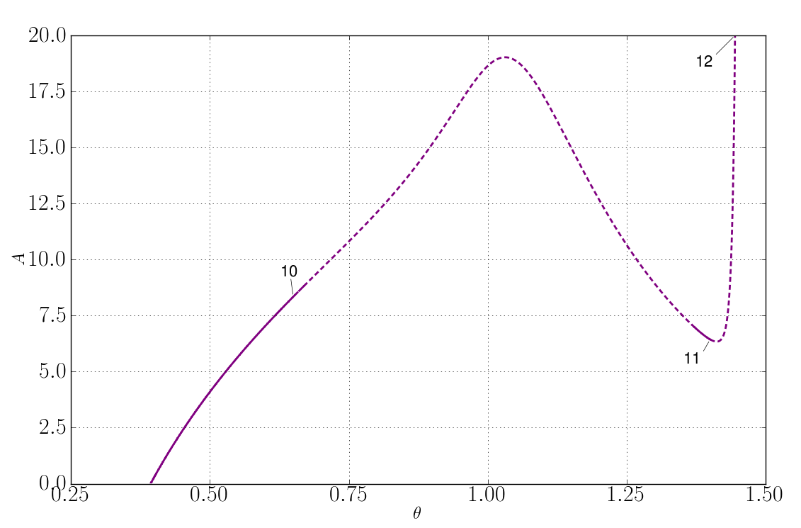
Figure 7: A continuum family of choreographies, for the case of 5 vortices on a sphere. Solid curve sections represent stable or almost stable choreographies. The solutions labeled $10$, $11$, and $12$ are shown in Figures 8 and 9. Further data can be found in Table 1.

The presence of the problem parameter $\theta$ allows for additional continuation schemes, as was the case in Section 4 for the disk, and in Section 5 for the case with a central vortex. For the sphere we have found it useful to continue resonant orbits found along primary families, keeping the resonance ratio fixed, as also done in Section 5. In particular, such secondary continuation can be used to determine a continuum of choreographies, as represented in Figure 7 for the case of $5$ vortices. The particular family shown there is obtained by first following one of the four families that bifurcate from the relative equilibrium when $\theta=\pi/5$, namely one of the two families that arise from the purely imaginary eigenvalue $2.78686i$ of multiplicity 2. Along this primary family we can detect an unlimited number of resonances that correspond to choreographies. Secondary continuation of one such a resonant orbit, namely one with $T/T_{0}=-33:26$, keeping the resonance fixed and allowing $\theta$ to vary, generates the family represented in Figure 7.

The base period $T_{0}$ of the rotating frame is taken to be a function of $\theta$, namely $T_{0}=2\pi/\omega$, where $\omega=\omega(r)$, and $r=\cot(\theta/2)$, with $\omega(r)$ defined in Equation 22. We also note that the sign of $T_{0}$, and correspondingly the sign of a resonance ratio, relates to the direction of rotation of the rotating frame. The orbits labeled $10$, $11$, and $12$ in Figure 7, of which the first two are stable, are shown in Figure 8 (the planar representation), and in Figure 9 (mapped onto the sphere); on the left in the rotating frame, and on the right in the inertial frame. As follows from the discussion above, all three have the same resonance ratio, namely, $T/T_{0}=-33:26$. We note that the path to the family of choreographies in Figure 7 could equally well have started from another polygonal equilibrium for another value of $\theta$.

The three panels on the left in Figure 10 show a selection of orbits along each of the three primary families that exist for the case of $n=4$ vortices. The families shown there arise from a polygonal equilibrium along the northern hemisphere, namely for $\theta=\pi/5$, which has purely imaginary eigenvalues $3.51246i$ (multiplicity $2$), and $2.84115i$ (multiplicity $1$), as well as two zero eigenvalues. We note that a corresponding polygonal equilibrium along the southern hemisphere, namely for $\theta=4\pi/5$, has the same eigenvalues, but with period of the rotating frame of opposite sign, namely $T_{0}=1.78883$ for the southern equilibrium, as opposed to $T_{0}=-1.78883$ for the corresponding northern equilibrium.

The primary family shown in the top-left panel of Figure 10 is one of the two families that arise from the double eigenvalue $3.51246i$. The orbits along this family are degenerate, in the sense that the period $T$ remains constant, with constant resonance ratio $T/T_{0}=-1$. In fact, all orbits of this family correspond to choreographies, albeit trivial ones, as they correspond to sliding a planar circular orbit along the sphere. Three such circular choreographies are shown in the top-right column of Figure 10. The primary family shown in the center-left panel of Figure 10 is the second family that arises from the double eigenvalues $3.51246i$. Both families from this eigenvalue were determined via the perturbation approach that was used earlier in this paper. One of the countably infinite number of choreographies that exist along this second family is shown in the center-right panel. The bottom-left panel of Figure 10 shows orbits along the third family that arises from the polygonal equilibrium, namely the family that arises from the multiplicity-1 eigenvalue $2.84115i$. This family can be computed directly, i.e., without use of the perturbation technique. Here also, one of the countably infinite number of choreographies along this family is shown in the bottom-right panel.

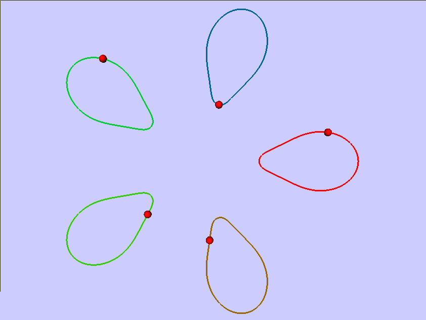
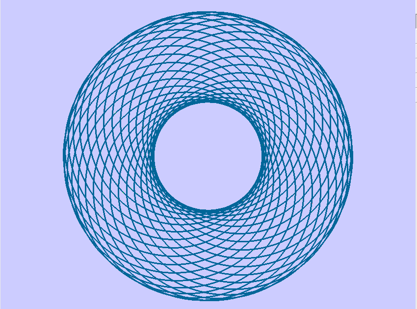
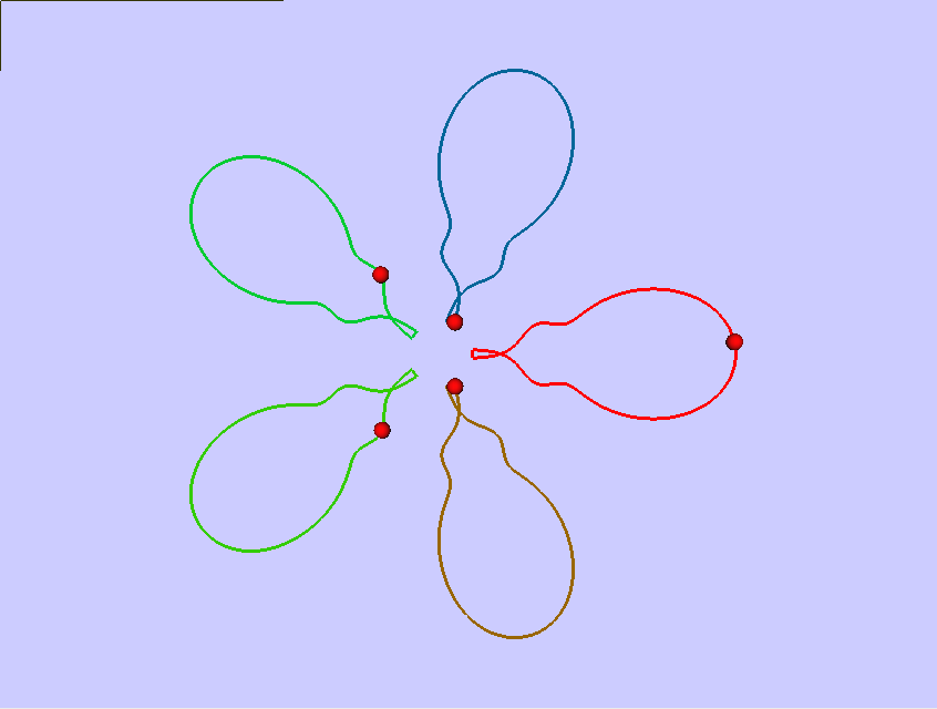
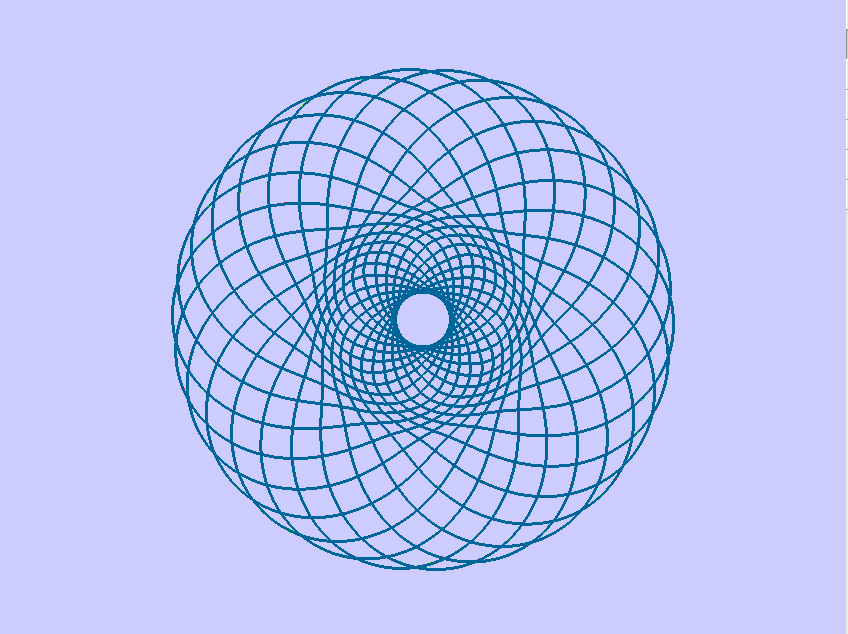
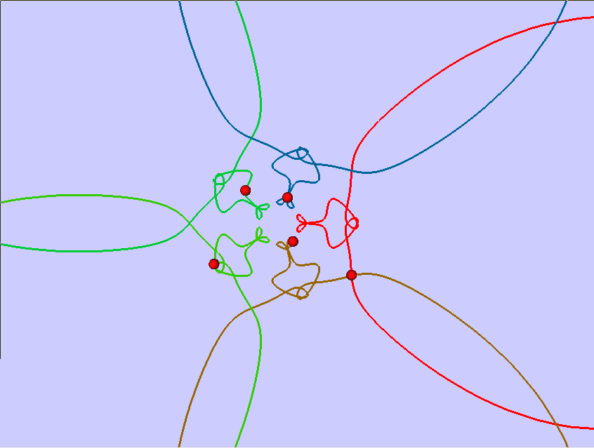
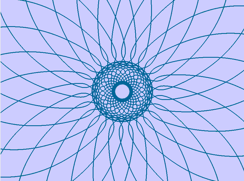
Figure 8: Row-wise: Solutions $10$, $11$ and $12$ from the continuum family of choreographies in Figure 7, for 5 vortices on a sphere, when stereographically projected onto the plane. The choreographies are shown on the left in the rotating frame, and on the right in the inertial frame. The orbits are drawn on a fixed scale, as a result of which the orbits in the third row are shown only partially. Numerical data can be found in Table 1.

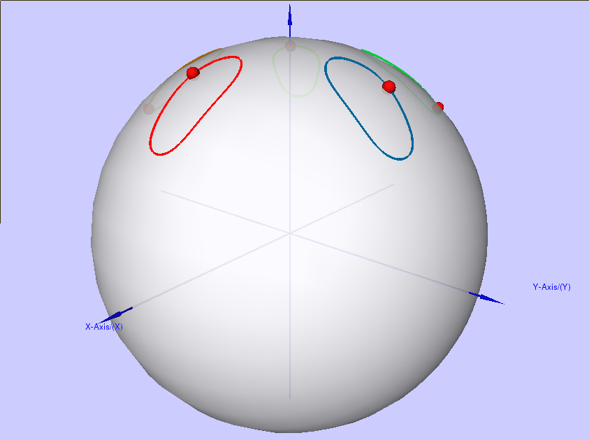
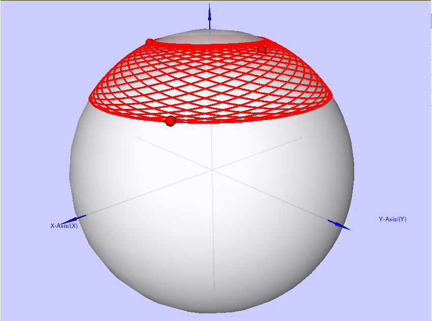
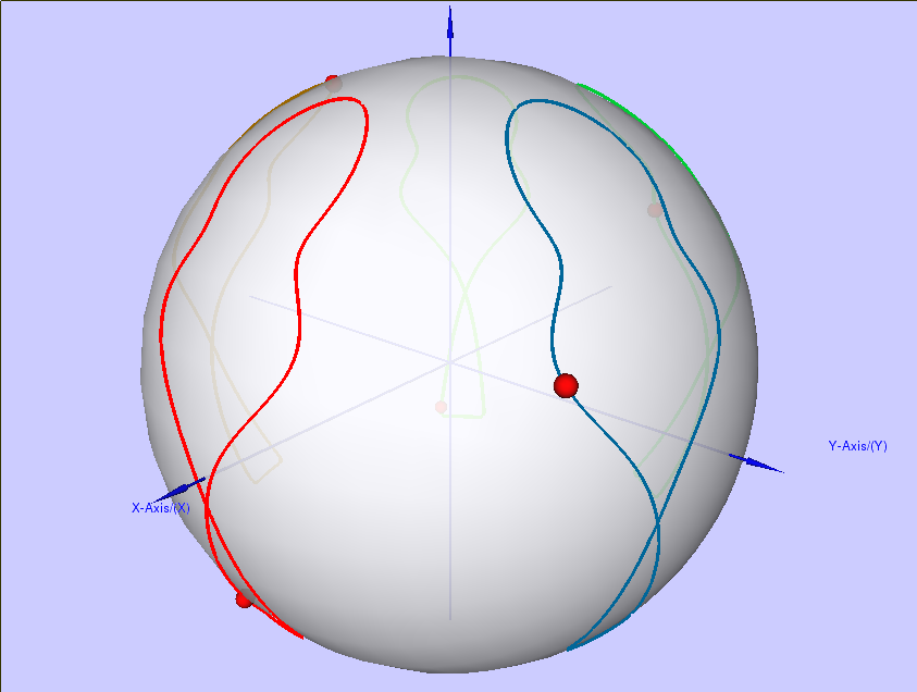
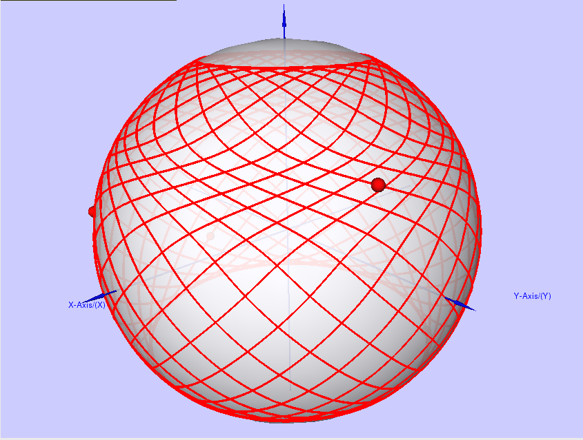
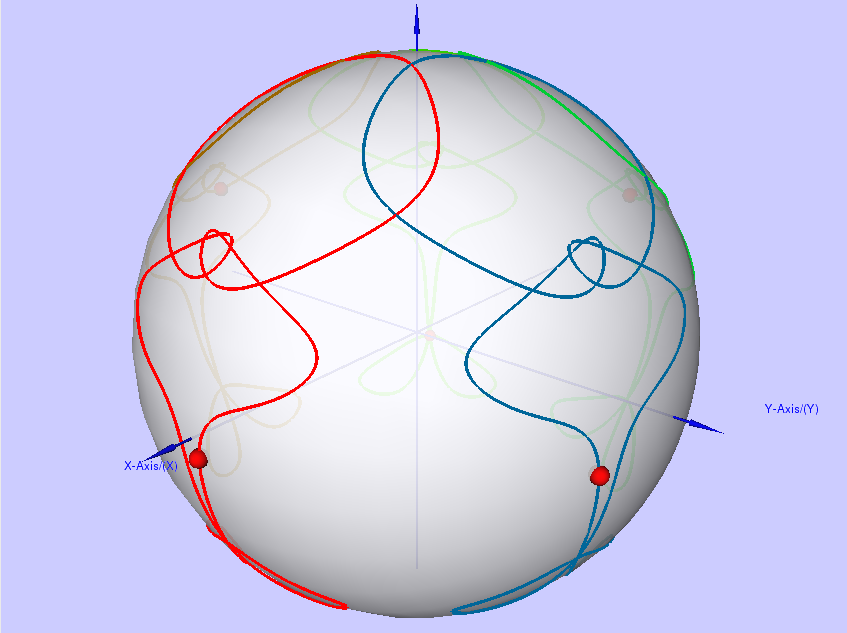
Figure 9: Row-wise: Solutions $10$, $11$ and $12$ from the continuum family of choreographies in Figure 7, as shown in their planar representation in Figure 8. Here these orbits are shown after being transformed back onto the sphere. The choreographies are shown on the left in the rotating frame, and on the right in the inertial frame. Numerical data can be found in Table 1.

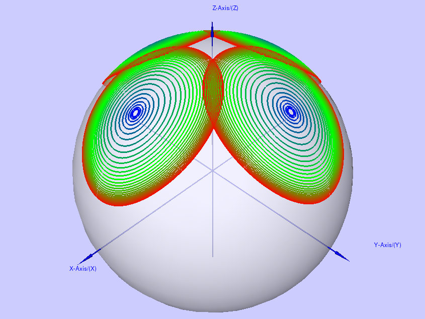
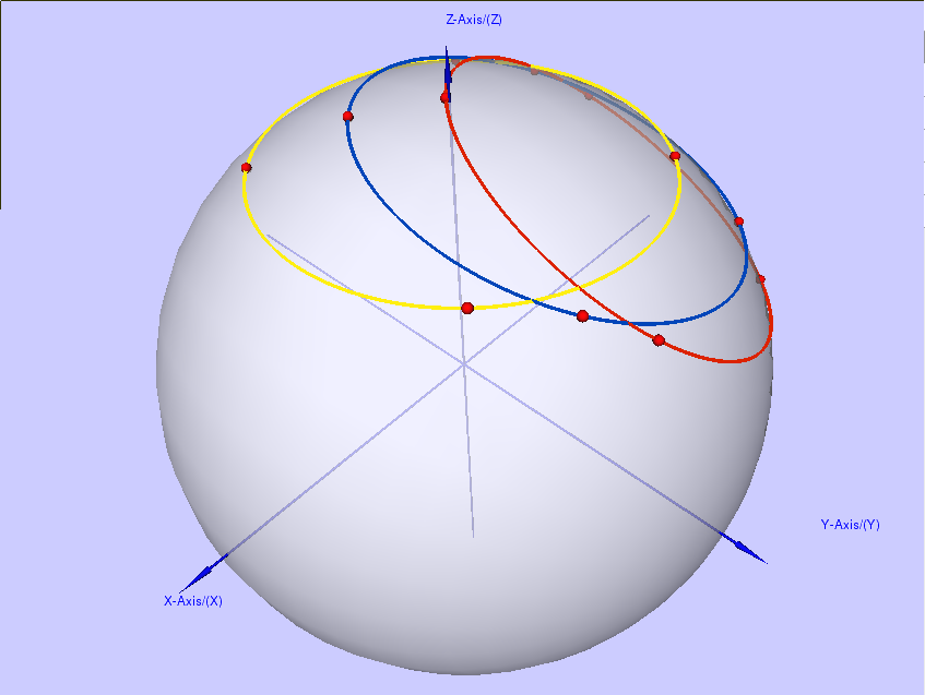
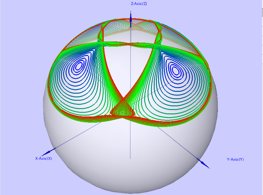
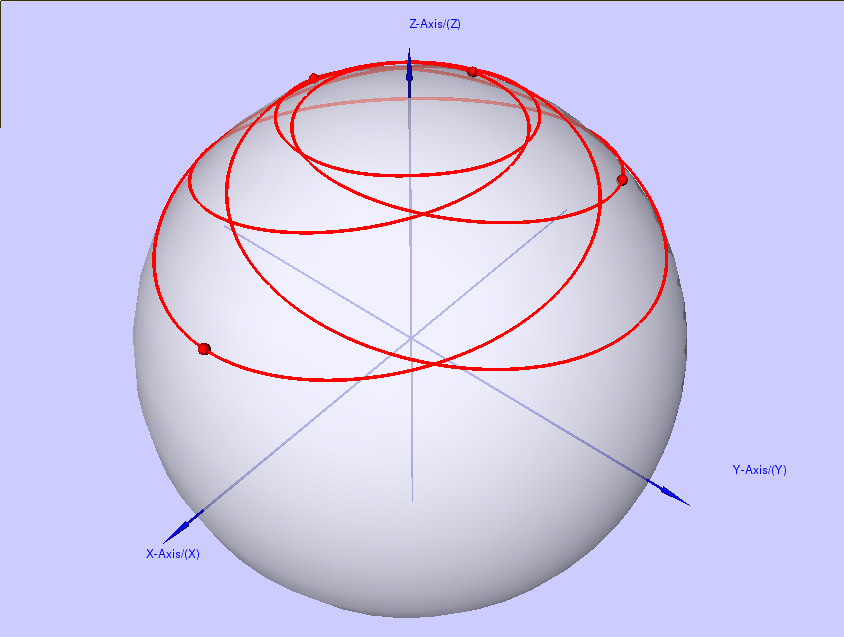
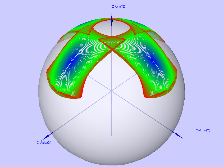
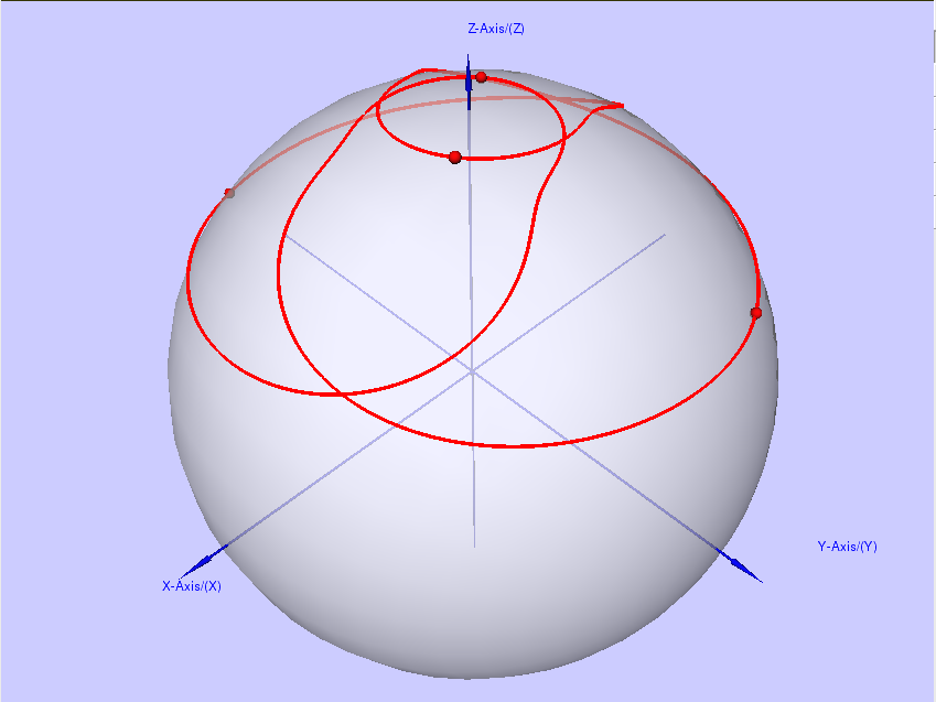
Figure 10: Left columns: The three primary families that bifurcate from the polygonal equilibrium for the case of $4$ vortices, with $\theta=\pi/5$. Right columns: Selected choreographies that occur along the primary families in the left column.

Figure	Row	Label	$n$	$T/T_{0}$	Parameter	$T$	$T_{0}$	Stable/
								Unstable
2	1	1	5	9:8		3.53429	3.14159	S
(plane)	2	2	5	33:26	(none)	3.98741	3.14159	S
	3	3	5	4:3		4.18879	3.14159	U
4	1	4	5	13:6	$R=1.99442$	6.78972	3.13372	S
(disk)	2	5	5	3:1	$R=1.85172$	9.37522	3.12507	U
	3	6	5	14:3	$R=1.75556$	14.5297	3.11350	S
6	1	7	5+1	11:4	$\mu=1.85436$	4.48291	1.63015	S
(with	2	8	5+1	11:4	$\mu=0.39014$	7.22918	2.62879	U
center
vortex)	3	9	5+1	11:4	$\mu=0.00500$	8.61784	3.13376	U
8	1	10	5	-33:26	$\theta=0.65$	1.83447	-1.44534	S
(sphere)	2	11	5	-33:26	$\theta=1.40$	22.7821	-17.9496	S
	3	12	5	-33:26	$\theta=1.44466$	31.1935	-24.5767	U

Table 1: Data for the orbits in Figures 1-8, where $n$ is the number of vortices, $T$ is the period of the orbit in the rotating frame, and $T_{0}$ the period of the rotating frame. The ”parameter” column shows the value of a physical parameter, which is absent in the case of vortices in the plane. Orbits are designated as “Stable” (S) when the largest Floquet multiplier is very close to the unit circle in the complex plane; otherwise they are listed as “Unstable” (U).

7 Conclusions

We have presented a systematic approach to the determination of choreographies of the $n$-vortex problem in the plane, in a disk and on a sphere. Our approach is based on the symmetries of the Lyapunov families of periodic orbits that bifurcate from the polygonal relative equilibrium in a rotating frame. The approach is similar to the one that we have used to find choreographies for the $n$-body problem [10]. We use highly accurate boundary value continuation techniques with adaptive meshes to compute the Lyapunov orbits, and we presented a small, but representative selection of the infinite number of choreographies that exists along the Lyapunov families. A choreography of the $n$-polygon in the plane is invariant under scaling, because the equations are homogeneous in that case. However, for a disk and a sphere, the $n$-vortex problem is not homogeneous. One of the interesting features of our results is therefore that in these cases we can determine a continuum of choreographies with fixed resonance ratio, where the choreographies are not related by scaling. Representative orbits from such continua are included in our presentation.

References

- [1] H. Aref, On the equilibrium and stability of a row of point vortices, J. Fluid Mech, 290 (1995), pp. 167-18l.
- [2] H. Aref, P. Newton, M. Stremler, T. Tokieda, D. Vainchtein. Vortex Crystals, Department of Theoretical and Applied Mechanics (UIUC), TAM Reports 2002.
- [3] H. Aref, N. Pomphrey, Integrable and chaotic motions of four vortices. I – The case of identical vortices, Proc. Roy. Soc. London Ser. A., 380 (1982), pp. 359–387.
- [4] T. Bartsch, Q. Dai, Periodic solutions of the N-vortex Hamiltonian system in planar domains, J. Differential Equations, 260(3) (2016), pp. 2275-2295.
- [5] T. Bartsch, B. Gebhard, Global continua of periodic solutions of singular first-order Hamiltonian systems of N-vortex type, Math. Ann., 369 (2017), pp. 627–651.
- [6] A. V. Borisov, I. S. Mamaev, A. A. Kilin, Absolute and relative choreographies in the problem of point vortices moving on a plane, Regular and Chaotic Dynamics, 9(2) (2004), pp. 101-11.
- [7] Borisov A. V., Mamaev I. S., Kilin A. A., New periodic solutions for three or four identical vortices on a plane and a sphere, Discrete and Continuous Dynamical Systems - Series B (Supplement Volume devoted to the 5th AIMS International Conference on Dynamical Systems and Differential Equations (Pomona, California, USA, June 2004)), 2005, pp. 110-120
- [8] Borisov A. V., Kilin A. A., Stability of Thomson’s Configurations of Vortices on a Sphere, Regular and Chaotic Dynamics, 2000, vol. 5, no. 2, pp. 189-200
- [9] H. E. Cabral and D. S. Schmidt, Stability of relative equilibria in the problem of N+1 vortices, SIAM J. Math. Anal., 31 (1999), pp. 231-250.
- [10] Calleja, R., Doedel, E. & García-Azpeitia, C. Symmetries and choreographies in families bifurcating from the polygonal relative equilibrium of the n-body problem. Celest Mech Dyn Astr 130: 48 (2018). https://doi.org/10.1007/s10569-018-9841-9
- [11] R. Calleja, E. Doedel, C. García-Azpeitia, Carlos L. Pando L., Choreographies in the discrete nonlinear Schrödinger equations, Eur. Phys. J. Special Topics, Special Issue on Nonlinear Phenomena in Physics: New Techniques and Applications (2018), in press.
- [12] A. C. Carvalho, H. E. Cabral. Lyapunov Orbits in the n-Vortex Problem. Regular and Chaotic Dynamics. 19(3) (2014) 348–362.
- [13] A. Chenciner, J. Fejoz, Unchained polygons and the n-body problem. Regular and chaotic dynamics, 14(1) (2009), pp. 64–115.
- [14] A. Chenciner, R. Montgomery, A remarkable periodic solution of the three-body problem in the case of equal masses, Ann. of Math., 152(2) (2000), pp. 881–901.
- [15] Q. Dai, B. Gebhard, T. Bartsch, Periodic Solutions of N-Vortex Type Hamiltonian Systems near the Domain Boundary, SIAM Journal on Applied Mathematics 78(2) (2018), pp. 977-995.
- [16] E. J. Doedel et al., AUTO-07p: Continuation and bifurcation software for ordinary differential equations. Concordia Univ. (2012) (http://sourceforge.net/projects/auto-07p/files/auto07p/).
- [17] E. J. Doedel, AUTO: A program for the automatic bifurcation analysis of autonomous systems. Cong. Num. 30 (1981), pp. 265-284, (Proc. 10th Manitoba Conf. on Num. Math. and Comp., Univ. of Manitoba, Winnipeg, Canada.)
- [18] H.-D. Ebbinghaus, A. Kanamori (Eds.), Ernst Zermelo - Collected Works/Gesammelte Werke II, Springer-Verlag, Berlin Heidelberg 2013, pp. 300-463.
- [19] C. García-Azpeitia, Relative periodic solutions of the -vortex problem on the sphere, Preprint arXiv:1805.10417.
- [20] C. García-Azpeitia, J. Ize, Global bifurcation of polygonal relative equilibria for masses, vortices and dNLS oscillators, J. Differential Equations, 251 (2011), pp. 3202–3227.
- [21] C. García-Azpeitia, J. Ize, Bifurcation of periodic solutions from a ring configuration in the vortex and filament problems, J. Differential Equations 252 (2012), pp. 5662-5678.
- [22] T.H. Havelock F.R.S. LII, The stability of motion of rectilinear vortices in ring formation, Philosophical Magazine Series 7, 11:70 (1931), pp. 617-633.
- [23] J. Ize, A. Vignoli, Equivariant degree theory. De Gruyter Series in Nonlinear Analysis and Applications 8, Walter de Gruyter, Berlin, 2003.
- [24] C. Lim, J. Montaldi and R.M. Roberts, Relative equilibria of point vortices on the sphere, Physica D, 148 (2001), pp. 97-135.
- [25] C. C. Lin, On the motion of vortices in 2D I. Existence of the Kirchhoff-Routh function, Proc. Nat. Acad. Sc., 27 (1941), pp. 570–575.
- [26] L. Kurakin. Point vortices in a circular domain: stability, resonances, and instability of stationary rotation of a regular vortex polygon. Congrès Français de Mécanique Grenoble, 27-31, 2007.
- [27] J. Montaldi, T. Tokieda, Deformation of Geometry and Bifurcations of Vortex Rings, Recent Trends in Dynamical Systems 335-370, Springer Basel 2013.
- [28] C. Moore, Braids in Classical Gravity. Physical Review Letters, 70 (1993), pp. 3675–3679.
- [29] F. Muñoz-Almaraz, E. Freire, J. Galán, E. Doedel, A. Vanderbauwhede. Continuation of periodic orbits in conservative and Hamiltonian systems. Phys. D 181 (2003), pp. 1–38.
- [30] P. K. Newton, The -vortex problem. Analytical techniques. Applied Mathematical Sciences, 145, Springer-Verlag, New York, 2001.
- [31] C. Simó, New Families of Solutions in N-Body Problems. European Congress of Mathematics 101–115, Springer Nature, 2001.