Towards Neural Theorem Proving at Scale

Abstract

Neural models combining representation learning and reasoning in an end-to-end trainable manner are receiving increasing interest. However, their use is severely limited by their computational complexity, which renders them unusable on real world datasets. We focus on the Neural Theorem Prover (NTP) model proposed by Rocktäschel and Riedel (2017), a continuous relaxation of the Prolog backward chaining algorithm where unification between terms is replaced by the similarity between their embedding representations. For answering a given query, this model needs to consider all possible proof paths, and then aggregate results – this quickly becomes infeasible even for small Knowledge Bases (KBs). We observe that we can accurately approximate the inference process in this model by considering only proof paths associated with the highest proof scores. This enables inference and learning on previously impracticable KBs.

1 Introduction

Recent advancements in deep learning intensified the long-standing interests in integrating symbolic reasoning with connectionist models (Shen, 1988; Ding et al., 1996; Garcez et al., 2012; Marcus, 2018). The attraction of said integration stems from the complementing properties of these systems. Symbolic reasoning models offer interpretability, efficient generalisation from a small number of examples, and the ability to leverage knowledge provided by an expert. However, these systems are unable to handle ambiguous and noisy high-dimensional data such as sensory inputs (Raedt and Kersting, 2008). On the other hand, representation learning models exhibit robustness to noise and ambiguity, can learn task-specific representations, and achieve state-of-the-art results on a wide variety of tasks (Bengio et al., 2013). However, being universal function approximators, these models require vast amounts of training data and are treated as non-interpretable black boxes.

One way of integrating the symbolic and sub-symbolic models is by continuously relaxing discrete operations and implementing them in a connectionist framework. Recent approaches in this direction focused on learning algorithmic behaviour without the explicit symbolic representations of a program (Graves et al., 2014, 2016; Kaiser and Sutskever, 2016; Neelakantan et al., 2016; Andrychowicz and Kurach, 2016), and consequently with it (Reed and de Freitas, 2016; Bosnjak et al., 2017; Gaunt et al., 2016; Parisotto et al., 2016). In the inductive logic programming setting, two new models, NTPs (Rocktäschel and Riedel, 2017) and Differentiable Inductive Logic Programming ($\partial$ILP) (Evans and Grefenstette, 2018) successfully combined the interpretability and data efficiency of a logic programming system with the expressiveness and robustness of neural networks.

In this paper, we focus on the NTP model proposed by Rocktäschel and Riedel (2017). Akin to recent neural-symbolic models, NTPs rely on a continuous relaxation of a discrete algorithm, operating over the sub-symbolic representations. In this case, the algorithm is an analogue to Prolog’s backward chaining with a relaxed unification operator. The backward chaining algorithm constructs neural networks, which model continuously relaxed proof paths using sub-symbolic representations. These representations are learned end-to-end by maximising the proof scores of facts in the KB, while minimising the score of facts not in the KB, in a link prediction setting (Nickel et al., 2016). However, while the symbolic unification checks whether two terms can represent the same structure, the relaxed unification measures the similarity between their sub-symbolic representations.

grandpaOf

abebart $\varnothing$ 1. $\varnothing$ 2. X/abe Y/bart 3. 3.1 ${\color[rgb]{0.4482421875,0.228515625,0.48046875}\verb~fatherOf~}({\color[rgb]{0.75,0.3720703125,0}\textsc{X}},{\color[rgb]{0.75,0.3720703125,0}\textsc{Z}})$ 3.2 ${\color[rgb]{0.4482421875,0.228515625,0.48046875}\verb~parentOf~}({\color[rgb]{0.75,0.3720703125,0}\textsc{Z}},{\color[rgb]{0.75,0.3720703125,0}\textsc{Y}})$

fatherOf

abeZ X/abe Y/bart Z/homer 3.2 ${\color[rgb]{0.4482421875,0.228515625,0.48046875}\verb~parentOf~}({\color[rgb]{0.75,0.3720703125,0}\textsc{Z}},{\color[rgb]{0.75,0.3720703125,0}\textsc{Y}})$1. X/abe Y/bart Z/bart 3.2 ${\color[rgb]{0.4482421875,0.228515625,0.48046875}\verb~parentOf~}({\color[rgb]{0.75,0.3720703125,0}\textsc{Z}},{\color[rgb]{0.75,0.3720703125,0}\textsc{Y}})$2.

FAIL

3.

parentOf

homerbart X/abe Y/bart Z/homer X/abe Y/bart Z/homer

FAIL

1.3.2.

parentOf

bartbart X/abe Y/bart Z/bart X/abe Y/bart Z/bart

FAIL

1.3.2.

Figure 1: A visual depiction of the NTP’ recursive computation graph construction, applied to a toy KB (top left). Dash-separated rectangles denote proof states (left: substitutions, right: proof score -generating neural network). All the non-FAIL proof states are aggregated to obtain the final proof success (depicted in Figure 2). Colours and indices on arrows correspond to the respective KB rule application.

This continuous relaxation is at the crux of NTPs’ inability to scale to large datasets. During both training and inference, NTPs need to compute all possible proof trees needed for proving a query, relying on the continuous unification of the query with all the rules and facts in the KB. This procedure quickly becomes infeasible for large datasets, as the number of nodes of the resulting computation graph grows exponentially.

Our insight is that we can radically reduce the computational complexity of inference and learning by generating only the most promising proof paths. In particular, we show that the problem of finding the facts in the KB that best explain a query can be reduced to a $k$-nearest neighbour problem, for which efficient exact and approximate solutions exist (Li et al., 2016). This enables us to apply NTPs to previously unreachable real-world datasets, such as WordNet.

2 Background

In NTPs, the neural network structure is built recursively, and its construction is defined in terms of modules similarly to dynamic neural module networks (Andreas et al., 2016). Each module, given a goal, a KB, and a current proof state as inputs, produces a list of new proof states, where the proof states are neural networks representing partial proof success scores.

Unification Module. In backward chaining, unification between two atoms is used for checking whether they can represent the same structure. In discrete unification, non-variable symbols are checked for equality, and the proof fails if the symbols differ. In NTPs, rather than comparing symbols, their embedding representations are compared by means of a Radial Basis Function (RBF) kernel. This allows matching different symbols with similar semantics, such as matching relations like ${\color[rgb]{0.4482421875,0.228515625,0.48046875}\verb~grandFatherOf~}$ and ${\color[rgb]{0.4482421875,0.228515625,0.48046875}\verb~grandpaOf~}$. Given a proof state $S=(S_{\psi},S_{\rho})$, where $S_{\psi}$ and $S_{\rho}$ denote a substitution set and a proof score, respectively, unification is computed as follows:

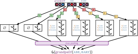
Figure 2: Depiction of the proof aggregation for the computation graph presented in Figure 1. Proof states resulting from the computation graph construction are all aggregated to obtain the final success score of proving a query.

$$1. \ \ {\color[rgb]{0.4482421875,0.228515625,0.48046875}\verb~unify~}_{{\bm{\theta}}}(\bm{[}\ \bm{]},\bm{[}\ \bm{]},S)=S$$

$$2. \ \ {\color[rgb]{0.4482421875,0.228515625,0.48046875}\verb~unify~}_{{\bm{\theta}}}(\bm{[}\ \bm{]},\textsc{G},S)=\verb~FAIL~$$

$$3. \ \ {\color[rgb]{0.4482421875,0.228515625,0.48046875}\verb~unify~}_{{\bm{\theta}}}(\textsc{H},\bm{[}\ \bm{]},S)=\verb~FAIL~$$

$$4. \ \ {\color[rgb]{0.4482421875,0.228515625,0.48046875}\verb~unify~}_{{\bm{\theta}}}(h::\textsc{H},g::\textsc{G},S)={\color[rgb]{0.4482421875,0.228515625,0.48046875}\verb~unify~}_{{\bm{\theta}}}(\textsc{H},\textsc{G},S^{\prime})$$

$$\ \ \ \ \text{with}\ \ S^{\prime}=(S^{\prime}_{\psi},S^{\prime}_{\rho})\ \ \text{where:}$$

$$S^{\prime}_{\psi}= S_{\psi}\cup\left\{\begin{array}[]{ll}\{h/g\}&\text{if }h\in\mathcal{V}\\ \{g/h\}&\text{if }g\in\mathcal{V},h\not\in\mathcal{V}\\ \varnothing&\text{otherwise}\end{array}\right\}$$

$$S^{\prime}_{\rho}= \min\left(S_{\rho},\left\{\begin{array}[]{ll}\operatorname{k}\left({{\bm{\theta}}}_{h:},{{\bm{\theta}}}_{g:}\right)&\text{if }h\not\in\mathcal{V},g\not\in\mathcal{V}\\ 1&\text{otherwise}\end{array}\right\}\right)$$

where ${{\bm{\theta}}}_{h:}$ and ${{\bm{\theta}}}_{g:}$ denote the embedding representations of $h$ and $g$, respectively.

OR Module. This module attempts to apply rules in a KB. The name of this module stems from the fact that a KB can be seen as a large disjunction of rules and facts. In backward chaining reasoning systems, the OR module is used for unifying a goal with all facts and rules in a KB: if the goal unifies with the head of the rule, then a series of goals is derived from the body of such a rule. In NTPs, we calculate the similarity between the rule and the facts via the unify operator. Upon calculating the continuous unification scores, OR calls AND to prove all sub-goals in the body of the rule.

$${\color[rgb]{0.4482421875,0.228515625,0.48046875}\verb~or~}^{\mathcal{K}}_{{\bm{\theta}}}(\textsc{G},d,S)=\bm{[}S^{\prime}\ |\ S^{\prime}\in{\color[rgb]{0.4482421875,0.228515625,0.48046875}\verb~and~}^{\mathcal{K}}_{{\bm{\theta}}}(\textsc{B},d,{\color[rgb]{0.4482421875,0.228515625,0.48046875}\verb~unify~}_{{\bm{\theta}}}(\textsc{H},\textsc{G},S)),$$

$$\textsc{H}\ {\color[rgb]{0.6708984375,0.076171875,0.08203125}\text{:--}}\ \textsc{B}\in\mathcal{K}\bm{]}$$

AND Module. This module is used for proving a conjunction of sub-goals derived from a rule body. It first applies substitutions to the first atom, which is afterwards proven by calling the OR module. Remaining sub-goals are proven by recursively calling the AND module.

$$1. \ \ {\color[rgb]{0.4482421875,0.228515625,0.48046875}\verb~and~}^{\mathcal{K}}_{{\bm{\theta}}}(\_,\_,\verb~FAIL~)=\verb~FAIL~$$

$$2. \ \ {\color[rgb]{0.4482421875,0.228515625,0.48046875}\verb~and~}^{\mathcal{K}}_{{\bm{\theta}}}(\_,0,\_)=\verb~FAIL~$$

$$3. \ \ {\color[rgb]{0.4482421875,0.228515625,0.48046875}\verb~and~}^{\mathcal{K}}_{{\bm{\theta}}}(\bm{[}\ \bm{]},\_,S)=S$$

$$4. \ \ {\color[rgb]{0.4482421875,0.228515625,0.48046875}\verb~and~}^{\mathcal{K}}_{{\bm{\theta}}}(\textsc{G}:\mathbb{G},d,S)=\bm{[}S^{\prime\prime}\ |\ S^{\prime\prime}\in{\color[rgb]{0.4482421875,0.228515625,0.48046875}\verb~and~}^{\mathcal{K}}_{{\bm{\theta}}}(\mathbb{G},d,S^{\prime}),$$

$$\ \ \ \ S^{\prime}\in{\color[rgb]{0.4482421875,0.228515625,0.48046875}\verb~or~}^{\mathcal{K}}_{{\bm{\theta}}}(\text{substitute}(\textsc{G},S_{\psi}),d-1,S)\bm{]}$$

For further details on NTPs and the particular implementation of these modules, see Rocktäschel and Riedel (2017)

After building all the proof states, NTPs define the final success score of proving a query as an $\operatorname*{arg\,max}$ over all the generated valid proof scores (neural networks).

Example 2.1.

Assume a KBs $\mathcal{K}$, composed of $|\mathcal{K}|$ facts and no rules, for brevity. Note that $|\mathcal{K}|$ can be impractical within the scope of NTP. For instance, Freebase (Bollacker et al., 2008) is composed of approximately 637 million facts, while YAGO3 (Mahdisoltani et al., 2015) is composed by approximately 9 million facts. Given a query $g\triangleq[{\color[rgb]{0.4482421875,0.228515625,0.48046875}\verb~grandpaOf~},{\color[rgb]{0.1611328125,0.369140625,0.5419921875}\textsc{abe}},{\color[rgb]{0.1611328125,0.369140625,0.5419921875}\textsc{bart}}]$, NTP compares its embedding representation – given by the embedding vectors of ${\color[rgb]{0.4482421875,0.228515625,0.48046875}\verb~grandpaOf~}$, abe, and bart – with the representation of each of the $|\mathcal{K}|$ facts.

The resulting proof score of $g$ is given by:

$$\max_{f\in\mathcal{K}} \;{\color[rgb]{0.4482421875,0.228515625,0.48046875}\verb~unify~}_{{\bm{\theta}}}(g,[f_{p},f_{s},f_{o}],(\varnothing,\rho))$$ (1)

$$=\max_{f\in\mathcal{K}}\;\min\big{\{}\rho,\operatorname{k}({{\bm{\theta}}}_{\scriptsize{\color[rgb]{0.4482421875,0.228515625,0.48046875}\verb~grandpaOf~}:},{{\bm{\theta}}}_{f_{p}:}),$$

$$\qquad\qquad\qquad\operatorname{k}({{\bm{\theta}}}_{{\color[rgb]{0.1611328125,0.369140625,0.5419921875}\textsc{abe}}:},{{\bm{\theta}}}_{f_{s}:}),\operatorname{k}({{\bm{\theta}}}_{{\color[rgb]{0.1611328125,0.369140625,0.5419921875}\textsc{bart}}:},{{\bm{\theta}}}_{f_{o}:})\big{\}},$$

where $f\triangleq[f_{p},f_{s},f_{o}]$ is a fact in $\mathcal{K}$ denoting a relationship of type $f_{p}$ between $f_{s}$ and $f_{o}$, ${{\bm{\theta}}}_{s:}$ is the embedding representation of a symbol $s$, $\rho$ denotes the initial proof score, and $\operatorname{k}({}\cdot{},{}\cdot{})$ denotes the RBF kernel. Note that the maximum proof score is given by the fact $f\in\mathcal{K}$ that maximises the similarity between its components and the goal $g$: solving the maximisation problem in Equation 1 can be equivalently stated as a nearest neighbour search problem. In this work, we use Approximate Nearest Neighbour Search (ANNS) during the forward pass for considering only the most promising proof paths during the construction of the neural network.

3 Nearest Neighbourhood Search

From Example 2.1, we can see that the inference problem can be reduced to a nearest neighbour search problem. Given a query $g$, the problem is finding the fact(s) in $\mathcal{K}$ that maximise the unification score. This represents a computational bottleneck, since it is very costly to find the exact nearest neighbour in high-dimensional Euclidean spaces, due to the curse of dimensionality (Indyk and Motwani, 1998). Exact methods are rarely more efficient than brute-force linear scan methods when the dimensionality is high (Ge et al., 2014; Malkov and Yashunin, 2016). A practical solution consists in ANNS algorithms, which relax the condition of the exact search by allowing a small number of mistakes. Several families of ANNS algorithms exist, such as Locality-Sensitive Hashing (LSH) (Andoni et al., 2015), Product Quantization (PQ) (Jégou et al., 2011), and Proximity Graphs (PGs) (Malkov et al., 2014). In this work we use Hierarchical Navigable Small World (HNSW) (Malkov and Yashunin, 2016; Boytsov and Naidan, 2013), a graph-based incremental ANNS structure which can offer much better logarithmic complexity scaling in comparison with other approaches.

4 Related Work

Many machine learning methods rely on efficient nearest neighbour search for solving specific sub-problems. Given the computational complexity of nearest neighbour search, approximate methods, driven by advanced index structures, hash or even graph-based approaches are used to speed up the bottleneck of costly comparison. ANNS algorithms have been used to speed up various sorts of machine learning models, including mixture model clustering (Moore, 1999), case-based reasoning (Wess et al., 1993) to Gaussian process regression (Shen et al., 2006), among others. Similarly to this work, Rae et al. (2016) also rely on approximate nearest neighbours to speed up Memory-Augmented neural networks. Similarly to our work, they apply ANNS to query the external memory (in our case the KB memory) for $k$ closest words. They present drastic savings in speed and memory usage. Though as of this moment, our speed savings are not as drastic, the memory savings we achieve are sufficient so that we can train on WordNet, a dataset previously considered out of reach of NTPs.

Table 1: AUC-PR results on Countries and MRR and HITS@$m$ on Kinship, Nations, and UMLS.

Dataset		Metric	Model
			NTP	NTP 2.0 ($k$ = 1)
Countries	S1	AUC-PR	$90.83\pm 15.4$	$\bm{97.04}\pm 4.47$
	S2	AUC-PR	$87.40\pm 11.7$	$\bm{90.92}\pm 4.44$
	S3	AUC-PR	$56.68\pm 17.6$	$\bm{85.55}\pm 7.10$
Kinship		MRR	$0.60$	$\bm{0.65}$
		HITS@1	$0.48$	$\bm{0.57}$
		HITS@3	$\bm{0.70}$	$0.69$
		HITS@10	$0.78$	$\bm{0.81}$
Nations		MRR	$0.75$	$\bm{0.81}$
		HITS@1	$0.62$	$\bm{0.73}$
		HITS@3	$\bm{0.86}$	$0.83$
		HITS@10	$\bm{0.99}$	$\bm{0.99}$
UMLS		MRR	$\bm{0.88}$	$0.76$
		HITS@1	$\bm{0.82}$	$0.68$
		HITS@3	$\bm{0.92}$	$0.81$
		HITS@10	$\bm{0.97}$	$0.88$

Table 2: Rules induced on WordNet, with a confidence above $0.5$.

Confidence	Rule
0.584	_domain_topic(X, Y)  :– _domain_topic(Y, X)
0.786	_part_of(X, Y)  :– _domain_region(Y, X)
0.929	_similar_to(X, Y)  :– _domain_topic(Y, X)
0.943	_synset_domain_topic(X, Y)  :– _domain_topic(Y, X)
0.998	_has_part(X, Y)  :– _similar_to(Y, X)
0.995	_member_meronym(X, Y)  :– _member_holonym(Y, X)
0.904	_domain_topic(X, Y)  :– _has_part(Y, X)
0.814	_member_meronym(X, Y)  :– _member_holonym(Y, X)
0.888	_part_of(X, Y)  :– _domain_topic(Y, X)
0.996	_member_holonym(X, Y)  :– _member_meronym(Y, X)
0.877	_part_of(X, Y)  :– _domain_topic(Y, X)
0.945	_synset_domain_topic(X, Y)  :– _domain_region(Y, X)
0.879	_part_of(X, Y)  :– _domain_topic(Y, X)
0.926	_domain_topic(X, Y)  :– _domain_topic(Y, X)
0.995	_has_instance(X, Y)  :– _type_of(Y, X)
0.996	_type_of(X, Y)  :– _has_instance(Y, X)

5 Experiments

We compared results obtained by our model, which we refer to as NTP 2.0, with those obtained by the original NTP proposed by Rocktäschel and Riedel (2017). Results on several smaller datasets – namely Countries, Nations, Kinship, and UMLS – are shown in Table 1. When unifying goals with facts in the KB, for each goal, we use ANNS for retrieving the $k$ most similar (in embedding space) facts, and use those for computing the final proof scores. We report results for $k=1$, as we did not notice sensible differences for $k\in\{2,5,10\}$. However, we noticed sensible improvements in the case of Countries, and an overall decrease in performance in UMLS. A possible explanation is that ANNS (with $k=1$), due to its inherently approximate nature, does not always retrieve the closest fact(s) exactly. This behaviour may be a problem in some datasets where exact nearest neighbour search is crucial for correctly answering queries. We also evaluated NTP 2.0 on WordNet (Miller, 1995), a KB encoding lexical knowledge about the English language. In particular, we use the WordNet used by Socher et al. (2013) for their experiments. This dataset is significantly larger than the other datasets used by Rocktäschel and Riedel (2017) – it is composed by 38.696 entities, 11 relations, and the training set is composed by 112,581 facts. In WordNet, the accuracies on the validation and test sets were 65.29% and 65.72%, respectively – which is on par with the Distance Model, a Neural Link Predictor discussed by Socher et al. (2013), which achieves a test accuracy of 68.3%. However, we did not consider a full hyper-parameter sweep, and did not regularise the model using Neural Link Predictors, which sensibly improves NTPs’ predictive accuracy (Rocktäschel and Riedel, 2017). A subset of the induced rules is shown in Table 2.

6 Conclusions

We proposed a way to sensibly scale up NTPs by reducing parts of their inference steps to ANNS problems, for which very efficient and scalable solutions exist in the literature.

References

- Rocktäschel and Riedel [2017] Tim Rocktäschel and Sebastian Riedel. End-to-end differentiable proving. In Advances in Neural Information Processing Systems 30, pages 3788–3800. 2017.
- Shen [1988] ZL Shen. A theoretical framework of fuzzy prolog machine. Fuzzy Computing-Theory, Hardware and Applications, 1988.
- Ding et al. [1996] Liya Ding, Hoon Heng Teh, Peizhuang Wang, and Ho Chung Lui. A prolog-like inference system based on neural logic—an attempt towards fuzzy neural logic programming. Fuzzy Sets and Systems, 82(2):235–251, 1996.
- Garcez et al. [2012] Artur S d’Avila Garcez, Krysia B Broda, and Dov M Gabbay. Neural-symbolic learning systems: foundations and applications. Springer Science & Business Media, 2012.
- Marcus [2018] Gary Marcus. Deep learning: A critical appraisal. CoRR, abs/1801.00631, 2018.
- Raedt and Kersting [2008] Luc De Raedt and Kristian Kersting. Probabilistic inductive logic programming. In Probabilistic Inductive Logic Programming - Theory and Applications, volume 4911 of Lecture Notes in Artificial Intelligence, pages 1–27. Springer, 2008.
- Bengio et al. [2013] Yoshua Bengio, Aaron C. Courville, and Pascal Vincent. Representation learning: A review and new perspectives. IEEE Trans. Pattern Anal. Mach. Intell., 35(8):1798–1828, 2013.
- Graves et al. [2014] Alex Graves, Greg Wayne, and Ivo Danihelka. Neural turing machines. CoRR, abs/1410.5401, 2014.
- Graves et al. [2016] Alex Graves, Greg Wayne, Malcolm Reynolds, Tim Harley, Ivo Danihelka, Agnieszka Grabska-Barwinska, Sergio Gomez Colmenarejo, Edward Grefenstette, Tiago Ramalho, John Agapiou, Adrià Puigdomènech Badia, Karl Moritz Hermann, Yori Zwols, Georg Ostrovski, Adam Cain, Helen King, Christopher Summerfield, Phil Blunsom, Koray Kavukcuoglu, and Demis Hassabis. Hybrid computing using a neural network with dynamic external memory. Nature, 538(7626):471–476, 2016.
- Kaiser and Sutskever [2016] Lukasz Kaiser and Ilya Sutskever. Neural gpus learn algorithms. In Proceedings of the International Conference on Learning Representations, 2016.
- Neelakantan et al. [2016] Arvind Neelakantan, Quoc V. Le, and Ilya Sutskever. Neural programmer: Inducing latent programs with gradient descent. In Proceedings of the International Conference on Learning Representations, 2016.
- Andrychowicz and Kurach [2016] Marcin Andrychowicz and Karol Kurach. Learning efficient algorithms with hierarchical attentive memory. CoRR, abs/1602.03218, 2016.
- Reed and de Freitas [2016] Scott E. Reed and Nando de Freitas. Neural programmer-interpreters. In Proceedings of the International Conference on Learning Representations (ICLR), 2016.
- Bosnjak et al. [2017] Matko Bosnjak, Tim Rocktäschel, Jason Naradowsky, and Sebastian Riedel. Programming with a differentiable forth interpreter. In Proceedings of the 34th International Conference on Machine Learning, ICML, volume 70, pages 547–556. PMLR, 2017.
- Gaunt et al. [2016] Alexander L Gaunt, Marc Brockschmidt, Rishabh Singh, Nate Kushman, Pushmeet Kohli, Jonathan Taylor, and Daniel Tarlow. Terpret: A probabilistic programming language for program induction. arXiv preprint arXiv:1608.04428, 2016.
- Parisotto et al. [2016] Emilio Parisotto, Abdel-rahman Mohamed, Rishabh Singh, Lihong Li, Dengyong Zhou, and Pushmeet Kohli. Neuro-symbolic program synthesis. arXiv preprint arXiv:1611.01855, 2016.
- Evans and Grefenstette [2018] Richard Evans and Edward Grefenstette. Learning explanatory rules from noisy data. Journal of Artificial Intelligence Research, 61:1–64, 2018.
- Nickel et al. [2016] Maximilian Nickel, Kevin Murphy, Volker Tresp, and Evgeniy Gabrilovich. A review of relational machine learning for knowledge graphs. Proceedings of the IEEE, 104(1):11–33, 2016.
- Li et al. [2016] Wen Li, Ying Zhang, Yifang Sun, Wei Wang, Wenjie Zhang, and Xuemin Lin. Approximate nearest neighbor search on high dimensional data - experiments, analyses, and improvement (v1.0). CoRR, abs/1610.02455, 2016.
- Andreas et al. [2016] Jacob Andreas, Marcus Rohrbach, Trevor Darrell, and Dan Klein. Learning to compose neural networks for question answering. In Kevin Knight et al., editors, NAACL HLT 2016, The 2016 Conference of the North American Chapter of the Association for Computational Linguistics: Human Language Technologies, pages 1545–1554. The Association for Computational Linguistics, 2016.
- Bollacker et al. [2008] Kurt D. Bollacker, Colin Evans, Praveen Paritosh, Tim Sturge, and Jamie Taylor. Freebase: a collaboratively created graph database for structuring human knowledge. In Proceedings of the ACM SIGMOD International Conference on Management of Data, SIGMOD, pages 1247–1250. ACM, 2008.
- Mahdisoltani et al. [2015] Farzaneh Mahdisoltani, Joanna Biega, and Fabian M. Suchanek. YAGO3: A knowledge base from multilingual wikipedias. In CIDR 2015, Seventh Biennial Conference on Innovative Data Systems Research, 2015.
- Indyk and Motwani [1998] Piotr Indyk and Rajeev Motwani. Approximate nearest neighbors: Towards removing the curse of dimensionality. In Jeffrey Scott Vitter, editor, Proceedings of the Thirtieth Annual ACM Symposium on the Theory of Computing, pages 604–613. ACM, 1998.
- Ge et al. [2014] Tiezheng Ge, Kaiming He, Qifa Ke, and Jian Sun. Optimized product quantization. IEEE Transactions on Pattern Analysis and Machine Intelligence, 36(4):744–755, 2014.
- Malkov and Yashunin [2016] Yury A. Malkov and D. A. Yashunin. Efficient and robust approximate nearest neighbor search using hierarchical navigable small world graphs. CoRR, abs/1603.09320, 2016.
- Andoni et al. [2015] Alexandr Andoni, Piotr Indyk, Thijs Laarhoven, Ilya P. Razenshteyn, and Ludwig Schmidt. Practical and optimal LSH for angular distance. In Corinna Cortes et al., editors, Advances in Neural Information Processing Systems 28: Annual Conference on Neural Information Processing Systems, pages 1225–1233, 2015.
- Jégou et al. [2011] Hervé Jégou, Matthijs Douze, and Cordelia Schmid. Product quantization for nearest neighbor search. IEEE Trans. Pattern Anal. Mach. Intell., 33(1):117–128, 2011.
- Malkov et al. [2014] Yury Malkov, Alexander Ponomarenko, Andrey Logvinov, and Vladimir Krylov. Approximate nearest neighbor algorithm based on navigable small world graphs. Inf. Syst., 45:61–68, 2014.
- Boytsov and Naidan [2013] Leonid Boytsov and Bilegsaikhan Naidan. Engineering efficient and effective non-metric space library. In Similarity Search and Applications - 6th International Conference, SISAP 2013, Proceedings, pages 280–293, 2013.
- Moore [1999] Andrew W Moore. Very fast em-based mixture model clustering using multiresolution kd-trees. In Advances in Neural information processing systems, pages 543–549, 1999.
- Wess et al. [1993] Stefan Wess, Klaus-Dieter Althoff, and Guido Derwand. Using kd trees to improve the retrieval step in case-based reasoning. In European Workshop on Case-Based Reasoning, pages 167–181. Springer, 1993.
- Shen et al. [2006] Yirong Shen, Matthias Seeger, and Andrew Y Ng. Fast gaussian process regression using kd-trees. In Advances in neural information processing systems, pages 1225–1232, 2006.
- Rae et al. [2016] Jack Rae, Jonathan J Hunt, Ivo Danihelka, Timothy Harley, Andrew W Senior, Gregory Wayne, Alex Graves, and Tim Lillicrap. Scaling memory-augmented neural networks with sparse reads and writes. In Advances in Neural Information Processing Systems, pages 3621–3629, 2016.
- Miller [1995] George A. Miller. Wordnet: A lexical database for english. Commun. ACM, 38(11):39–41, 1995.
- Socher et al. [2013] Richard Socher, Danqi Chen, Christopher D. Manning, and Andrew Y. Ng. Reasoning with neural tensor networks for knowledge base completion. In Christopher J. C. Burges et al., editors, Advances in Neural Information Processing Systems 26: 27th Annual Conference on Neural Information Processing Systems, pages 926–934, 2013.