Randomness quantification of coherent detection

Abstract

Continuous-variable quantum cryptographic systems, including random number generation and key distribution, are often based on coherent detection. The essence of the security analysis lies in the randomness quantification. Previous analyses employ a semi-quantum picture, where the strong local oscillator limit is assumed. Here, we investigate the randomness of homodyne detection in a full quantum scenario by accounting for the shot noise in the local oscillator, which requires us to develop randomness measures in the infinite-dimensional scenario. Similar to the finite-dimensional case, our introduced measure of randomness corresponds to the relative entropy of coherence defined for an infinite-dimensional system. Our results are applicable to general coherent detection systems, in which the local oscillator is inevitably of finite power. As an application example, we employ the analysis method to a practical vacuum-fluctuation quantum random number generator and explore the limits of generation rate given a continuous-wave laser.

I Introduction

Quantum cryptography, the most practical field in quantum information science, has two major tasks — key distribution and randomness generation. Quantum key distribution (QKD) allows communication partners to share private keys in the presence of an eavesdropper, Eve, whose power is only limited by quantum mechanics Bennett and Brassard (1984); Ekert (1991). Quantum random number generation (QRNG) aims at providing unpredictable random numbers Ma et al. (2016); Herrero-Collantes and Garcia-Escartin (2017). The main theoretical focus of both cryptographic tasks lies in the security analysis, which ensures that Eve cannot predict the key or random numbers. Mathematically, the definitions of privacy in the key bits and unpredictability in the random numbers are the same. Thus, it is expected that security analyses in QKD can also be applied to QRNG and vice versa.

There are mainly two categories of schemes for quantum cryptographic systems, namely, discrete variable and continuous variable. Continuous-variable cryptography Grosshans and Grangier (2002); Grosshans et al. (2003) employs Gaussian modulation and coherent detection, e.g., homodyne detection and heterodyne detection. These are standard techniques in classical telecommunications, which could make continuous-variable optical components robust and economic. From the theoretical point of view, it is crucial to study the mechanism of coherent detection for the security analysis of continuous-variable cryptography. Without loss of generality, we will focus on continuous-variable QRNG systems below. Similar results should also be applicable to QKD systems.

Continuous-variable QRNG schemes Gabriel et al. (2010); Shen et al. (2010); Symul et al. (2011); Jofre et al. (2011); Shi et al. (2016); Marangon et al. (2017); Xu et al. (2017); Haylock et al. (2018); Guo et al. (2018); Avesani et al. (2018); Zheng et al. (2018); Fürst et al. (2010); Yan et al. (2014); Qi et al. (2010); Xu et al. (2012); Nie et al. (2014, 2015); Zhang et al. (2016a); Yang et al. (2016); Sun and Xu (2017) offer some advantage over conventional discrete-variable ones Jennewein et al. (2000); Stefanov et al. (2000); Cao et al. (2015, 2016) in both performance and practicality, especially the ones exploiting quadrature fluctuations of optical fields Gabriel et al. (2010); Shen et al. (2010); Symul et al. (2011); Jofre et al. (2011); Shi et al. (2016); Marangon et al. (2017); Xu et al. (2017); Haylock et al. (2018); Guo et al. (2018); Avesani et al. (2018); Zheng et al. (2018) or laser phase fluctuations Qi et al. (2010); Xu et al. (2012); Nie et al. (2014, 2015); Zhang et al. (2016a); Yang et al. (2016); Sun and Xu (2017), pushing the generation rate from Mbps to the Gbps regime. The substantial improvement in randomness generation performance is mainly attributed to the coherent detection technique, which replaces single-photon detectors with high-performance photodetectors, gets rid of the restriction of detector dead time, and yields a higher sampling rate.

For these continuous-variable QRNG schemes based on coherent detection, a physical model from the first principle along with rigorous randomness quantification is still missing. Former models of coherent detection QRNGs assumed that the local oscillator in use behaves classically Gabriel et al. (2010); Shen et al. (2010); Symul et al. (2011); Jofre et al. (2011); Shi et al. (2016); Marangon et al. (2017); Xu et al. (2017); Haylock et al. (2018); Guo et al. (2018); Avesani et al. (2018); Zheng et al. (2018); Ma et al. (2013); Zhou et al. (2015). In that case, by controlling the phase of the local oscillator $\phi$, different quadratures $\hat{x}(\phi)=1/2(\hat{a}e^{-i\phi}+\hat{a}^{{\dagger}}e^{i\phi})$ of the incoming mode of light, with annihilation operator $\hat{a}$, can then be measured. This leads to a continuum of measurement outcomes implying that the amount of randomness extracted from single round of detection is divergent with high detection resolution, which is rather counter-intuitive. Another issue lies in randomness quantification, where conventional approaches are based on classical min-entropy function Gabriel et al. (2010); Shen et al. (2010); Qi et al. (2010); Xu et al. (2012); Nie et al. (2015); Zhang et al. (2016a). Such quantifiers may suffer from side information in the measurement outcomes, i.e., the quantum state before measurement may be entangled with some ancillary systems held by the adversary. Though the nominal output randomness can be calculated by the measurement statistics, the intrinsic randomness that comes from quantum measurement stays unknown.

In this work, we properly model the coherent detection and provide a rigorous analysis of the randomness origin, quantification, and fundamental limits. By modelling the local oscillator quantum mechanically with a pure coherent state, we can look more closely at the mechanism of the coherent detection. What a coherent detection would effectively measure is the photon number difference between different legs. In this case, we can argue that the randomness in the outcome is a result of the shot-noise effect in the photodetection. For that reason, we refer to the continuous-variable QRNG scheme with coherent detection by shot-noise driven QRNG, whose measurement outcomes form a discrete, rather than continuous, infinite-dimensional space.

Meanwhile, in order to accurately calculate the intrinsic randomness in such a QRNG, we apply the rigorous and powerful tool of quantum coherence Baumgratz et al. (2014), which has been related to quantum randomness in Yuan et al. (2015). For instance, in the quantum information context, the $Z$-basis measurement on the qubit $(|0\rangle+|1\rangle)/\sqrt{2}$ would result in either basis states with equal probability. The result of such a measurement is unpredictable. A simple implementation of this idea is based on measuring the relative phase or polarization of a single photon Stefanov et al. (2000). One can get a similar result if, instead of a superposed state, a mixed state $(\mbox{$\left|0\right\rangle$}\mbox{$\left\langle 0\right|$}+\mbox{$\left|1\right\rangle$}\mbox{$\left\langle 1\right|$})/2$ is measured. In the latter case, however, we cannot rule out the possibility of the input state being entangled with another external system. In fact, we can purify our mixed state into a Bell state, in which case, an adversary party, who may hold the other part of the Bell state, can fully predict the outcome of the measurement. There is, in fact, no intrinsic (unpredictable) quantum randomness in this mixed-state case, and it only represents sheer classical randomness. The transition from fully random in the case of the superposition state to no quantum randomness for the mixed state indicates a correspondence between coherence of a state and how much quantum randomness can be extracted from it. In fact, it has been shown that, for finite-dimensional states, the relative entropy of coherence is an intrinsic randomness quantifier Yuan et al. (2016). In this paper, we extend this result to the infinite dimensional case and quantify the randomness in shot-noise driven QRNG with the help of infinite dimensional coherence Zhang et al. (2016b). We believe such an analysis should be a standard approach for randomness quantification of QRNGs based on coherent detection, and be further widely employed in other continuous-variable cryptography systems.

The rest of this paper is organised as follows. In Sec. II.1, we review the shot-noise driven QRNG structure and show that to properly quantify its generated randomness, we need to employ relevant measures for discrete infinite dimensional variables. Such measures are derived in Sec. II.2 and their correspondence with infinite dimensional coherence on Fock basis is shown. We then quantify the randomness in shot-noise driven QRNGs and find practical rate bounds for its realistic implementations in Sec. III before concluding the paper in Sec. IV.

II Shot-Noise Driven QRNG

II.1 Physical model of homodyne detection

Here we first focus on a shot-noise driven QRNG model which is based on homodyne detection of a vacuum state. A slightly modified version of this model can also be applied to other coherent detections, such as heterodyne detection. A schematic diagram of homodyne detection is shown in Fig. 1(a). A local oscillator (LO) in coherent state $|\alpha_{\rm LO}\rangle$ is coupled to a vacuum state at a 50:50 beam splitter (BS). The two output modes are then measured by two identical photodetectors. The resulting currents are subtracted from each other and converted to bits by an analogue-to-digital converter (ADC).

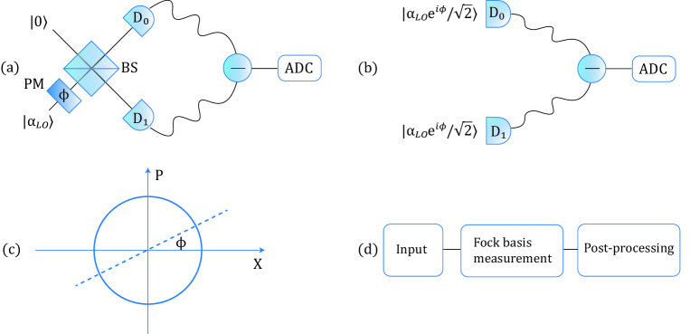
Figure 1: (a) Schematic diagram of a shot-noise driven QRNG. A homodyne receiver measures a certain quadrature $x(\phi)$ of the vacuum state, which is controlled by the phase modulator. (b) Equivalent setting of (a). The two input coherent states $\left|\alpha_{LO}e^{i\phi}/\sqrt{2}\right\rangle$ have the same phase, but their intensities are independent. The output is proportional to the photon-number difference measured by the two detectors. Here, the randomness originates from the shot-noise effect. (c) Phase space presentation of classical modelled homodyne detection measuring $x(\phi)$ quadrature of a vacuum state. (d) Generalized flow chart of a shot-noise driven QRNG. The whole process can be divided into a quantum phase performing Fock basis measurement on certain input states and a classical phase performing a post-processing on the Fock basis measurement outcomes. LO: local oscillator; PM: phase modulator; BS: beam splitter; $D_{0,1}$: photo detector; ADC: analogue-to-digital converter.

Such a process is expected to introduce random numbers. In previous analyses Gabriel et al. (2010); Symul et al. (2011); Shen et al. (2010); Shi et al. (2016), the LO is modelled classically as a plane wave (in the limit of strong LOs). We show the detailed classical description in Appendix A. This device practically measures $\hat{x}(\phi)$ quadrature of the vacuum state following Gaussian distribution, where $\phi$ is the modulated phase of the LO. In phase space, such a measurement is a cross-section of the Wigner function of the vacuum state (Fig. 1(c)).

Now, more precisely, we quantum mechanically characterize the LO as a pure coherent state

$$\mbox{$\left|\alpha_{\rm LO}\right\rangle$}=e^{-\frac{|\alpha_{\rm LO}|^{2}}{2}}\sum_{n}\frac{\alpha_{\rm LO}^{n}}{\sqrt{n!}}\mbox{$\left|n\right\rangle$},$$ (1)

where $\alpha_{\rm LO}$ is a complex number and $\left|n\right\rangle$ is a Fock state with $n$ photons. Then we can model the module in Fig. 1(a) by that of Fig. 1(b). Each photodetector performs a Fock basis measurement on $\left|\alpha_{\rm LO}e^{i\phi}/\sqrt{2}\right\rangle$. Because of the shot-noise effect, the output of both Fock basis measurements would follow a Poisson distribution

$$p^{\mathcal{P}}_{j}(\mu) =|\langle j|\alpha_{\rm LO}e^{i\phi}/\sqrt{2}\rangle|^{2}$$ (2)

$$=e^{-\mu}\frac{\mu^{j}}{j!},$$

with a mean of $\mu=|\alpha_{\rm LO}|^{2}/2$ and independent of the modulated phase $\phi$. If we denote the measured photon number by detector $D_{i}$, $i=0,1$, by $N_{i}$, the input to the ADC would then be proportional to the photon number difference $N_{d}=N_{0}-N_{1}$. It can be shown that $N_{d}$, as a difference of two independent Poisson distributions, follows Skellam distribution Skellam (1945) given by

$$p^{\mathcal{S}}_{j}(\mu) =\Pr(N_{d}=j)$$ (3)

$$=\left\{\begin{aligned} e^{-2\mu}I_{j}(2\mu)&\quad j>0\\ e^{-2\mu}I_{-j}(2\mu)&\quad j<0\end{aligned}\right.$$

where $I_{j}(2\mu)$ is the modified Bessel function given by Abramowitz et al. (1966)

$$I_{j}(2\mu)=\sum_{m=0}^{\infty}\frac{1}{m!\Gamma(m+j+1)}{\mu}^{2m+j}.$$ (4)

Figure 2 shows the Skellam distribution at $\mu=50$. It can be seen that it has a symmetric form getting its maximum value at $j=0$. For sufficiently large values of $\mu$, the Skellam distribution can be well approximated by a Gaussian distribution.

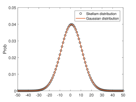
Figure 2: Comparison of a Skellam distribution, given in Eq. (3), and a Gaussian distribution, with the same mean $0$ and variance $2\mu=100$.

Our physical model of shot-noise driven QRNG can be easily generalized into coherent states input and general coherent detections (homodyne detection and heterodyne detection). For example, in homodyne detection, an $X$ quadrature measurement on the coherent state input $\left|\beta\right\rangle$ leads to a Skellam distribution of

$$p_{j}(\mu_{1},\mu_{2})=e^{-(\mu_{1}+\mu_{2})}\left(\frac{\mu_{1}}{\mu_{2}}\right)^{j/2}I_{j}(2\sqrt{\mu_{1}\mu_{2}}).$$ (5)

where $\mu_{1}$ and $\mu_{2}$, where

$$\mu_{1} =\frac{|\beta+\alpha_{LO}|^{2}}{2},$$ (6)

$$\mu_{2} =\frac{|\beta-\alpha_{LO}|^{2}}{2}.$$

and if we replace homodyne detection with heterodyne detection, there are two output Skellam distributions $p_{j}(\mu_{3},\mu_{4})$ and $p_{j}(\mu_{5},\mu_{6})$ where

$$\mu_{3,4} =|\frac{\beta}{2}\pm\frac{\alpha_{LO1}}{\sqrt{2}}|^{2}$$ (7)

$$\mu_{5,6} =|\frac{\beta}{2}\pm\frac{\alpha_{LO2}}{\sqrt{2}}|^{2}$$

Here $\left|\alpha_{LO1}\right\rangle$ and $\left|\alpha_{LO2}\right\rangle$ are local oscillators in heterodyne detection. For simplicity, we analyse the vacuum input and homodyne detection in the following text, but the methods for other cases are the same.

To fundamentally study the quantum randomness generated by the shot-noise driven QRNG, we have to separate classical sources of randomness from the underlying quantum phenomena. In our case, the electric noise of the receiver, for instance, would contribute to classically generated randomness and needs to be extracted out using distillation techniques. True intrinsic randomness comes from the photon number difference explained above. We then deal with an infinite dimensional, but discrete, random variable. In the next section, we derive a proper measure of randomness for such cases.

II.2 Randomness origin and quantification: infinite dimensional coherence

Now we consider the randomness origin and quantification in the shot-noise driven QRNG based on coherent detection. Figure. 1(d) schematically shows its mechanism, including a quantum phase performing Fock basis measurement on certain input states and a classical phase performing a post-processing on the Fock basis measurement outcomes. Same as finite dimensional case, the true randomness origins from the Fock basis measurement breaking the infinite dimensional coherence, which cannot be directly detected as raw data since the classical noises dominates. The post-processing, subtracting the two measurement results, is able to mitigate the classical noises and let the proportion of quantum signals high enough to be detected.

We begin the randomness quantification with the quantum version of min entropy function and show that, in the asymptotic limit, when an experiment is repeated infinitely many times, the average randomness per round approaches the Shannon entropy function. Consider an arbitrary state $\rho_{A}$, after a projective measurement $\left|i\right\rangle$$\left\langle i\right|$ on A, $\rho_{A}$ is dephased to $\rho_{A}^{\prime}=\sum_{i}p_{i}\mbox{$\left|i\right\rangle$}\mbox{$\left\langle i\right|$}$ in the measurement basis. In the worst case, the adversary is access to the most side information of the measurement outcomes by holding a purification of $\rho_{AE}=\mbox{$\left|\Psi\right\rangle$}_{AE}\mbox{$\left\langle\Psi\right|$}_{AE}$. And the state after measurement is $\rho_{A^{\prime}E}=\sum_{i}p_{i}\mbox{$\left|i\right\rangle$}\mbox{$\left\langle i\right|$}\otimes\rho_{E}^{i}$. The one-shot randomness in the measurement outcome against such an adversary is given by conditional min-entropy Tomamichel (2012)

$$S_{min}(A^{\prime}|E)=\max_{\sigma_{E}}\sup\{\lambda\in\mathcal{R}:\rho_{A^{\prime}E}\leq 2^{-\lambda}I_{A}\otimes\sigma_{E}\},$$ (8)

where the dimension of $\sigma_{E}$ is not higher than that of $\rho_{E}=\mathrm{tr}_{E}(\rho_{AE})$. In Appendix B, we prove that when $\rho_{A}$ is pure, this formula will reduce to the classical min-entropy function $H_{min}=-\log_{2}(\max_{i}p_{i})$. The $\epsilon$-smooth version of Eq. (8), removing extreme events, is also a one-shot randomness quantifier,

$$S^{\epsilon}_{min}(A^{\prime}|E)=\max_{\tilde{\rho_{AE}}}S_{min}(A^{\prime}|E)$$ (9)

satisfying $\sqrt{1-F^{2}(\tilde{\rho}_{AE},\rho_{AE})}\leq\epsilon$, where fidelity function is defined as $F(\tilde{\rho}_{AE},\rho_{AE})=\mathrm{tr}(\tilde{\rho}_{AE}\rho_{AE})$.

If the measurement is conducted $n$ times, in an independent and identical way, then the outputs are also independent and identically distributed (i.i.d) variables whose randomness is given by $S^{\epsilon}_{min}(A^{\prime n}|E^{n})$. In the limit of $n\rightarrow\infty$, for any $0<\epsilon<1$

$$\lim_{n\rightarrow\infty}\frac{1}{n}S^{\epsilon}_{min}(A^{\prime n}|E^{n})=S(A^{\prime}|E)=S(A^{\prime})-S(A)$$ (10)

where the first equation is the asymptotic equipartition property Tomamichel (2012), the second equation is referred to Ref. Yuan et al. (2016) for finite dimensional cases, but it still holds for infinite dimensional cases since the relative entropy of coherence is a well-defined coherence measure for infinite dimensional states Zhang et al. (2016b). Therefore, we can conclude that the randomness after the Fock basis measurement can be quantified with relative entropy of coherence. Fortunately, in our shot-noise driven QRNG, the state $\rho_{A}$ is a pure coherent state, the relative entropy of coherence reduce to Shannon entropy of the probability distribution of the measurement results,

$$R_{0} =C(\rho_{A})=H(\{p^{\mathcal{P}}_{j}(\mu)\})$$ (11)

$$=-\sum_{j=-\infty}^{\infty}p^{\mathcal{P}}_{j}(\mu)\log_{2}{p^{\mathcal{P}}_{j}(\mu)},$$

where $p^{\mathcal{P}}_{j}(\mu)$ is given by Eq. (2). After the post-processing of subtraction, the final randomness becomes

$$R_{1} =H(\{p^{\mathcal{S}}_{j}(\mu)\})$$ (12)

$$=-\sum_{j=-\infty}^{\infty}p^{\mathcal{S}}_{j}(\mu)\log_{2}{p^{\mathcal{S}}_{j}(\mu)},$$

which is less than the total randomness $2R_{0}$ and $p^{\mathcal{S}}_{j}(\mu)$ is given by Eq. (3). We compare the randomness before and after the subtraction, i.e., $2R_{0}$ and $R_{1}$ respectively, with respect to the intensity of the local oscillator in Fig. 3.

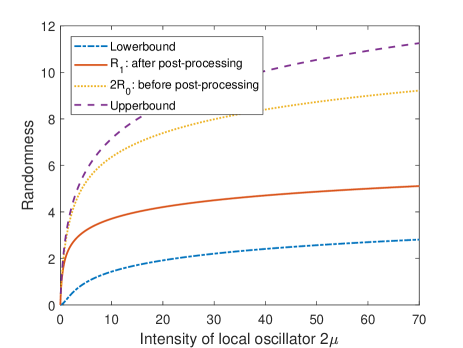
Figure 3: Dependence of the randomness before and after the post-processing of subtraction on the intensity of LO. In the legend “$R_{1}$: after post-processing” refers to Eq. (12) and “$2R_{0}$: before post-processing” refers to Eq. (11). The dashed line and dot-dashed line are practical upper and lower bound of randomness per sample given in Sec. III, respectively.

III Practical bounds for realistic implementations

In the last section, we obtained the random number generation rate for the shot-noise driven QRNG in Eq. (12). In this section, we try to find an upper bound $R^{U}$ and a lower bound $R^{L}$ on Eq. (12) for practical cases. The upper bound $R^{U}$ provides a limit on the output randomness per sample, while the lower bound $R^{L}$ is just randomness quantification in previous works Gabriel et al. (2010); Shen et al. (2010). In the following analysis, we model some experimental parameters relevant to realistic setups. In what follows, the power of the local oscillator, which is assumed to be generated by a continuous-wave laser, by $P$, central and max frequency of the laser by $\nu$ and $\nu_{m}$, the response time of the photodetectors by $\tau$, the sampling frequency of ADC by $f$, and the quantization interval of ADC by $a$.

III.1 Upper bound

The photon number of the LO within the response time follows Poisson distribution $p^{\mathcal{P}}_{j}(2\mu)$, where $2\mu=P\tau/(h\nu)$ is the mean photon number. The total randomness comes from two aspects, the randomness in the detection outcomes and the randomness in the Poisson distribution, i.e., $H(AB)=H(A|B)+H(B)$, where $A$ and $B$ stand for the two aspects above respectively. The maximum possible randomness for $n$-photon input is that the photon number difference $\{-n,-n+2,\cdots,n-2,n\}$ follows a uniform distribution, which corresponds to the max-entropy $\log_{2}(n+1)$. Then $H(A|B)<\sum_{n}p_{n}\log_{2}(n+1)\leq\log_{2}[(\sum_{n}p_{n}n)+1]$, where the second inequality is due to the concavity of logarithm function. Therefore we obtain an upper bound of randomness per sample,

$$R^{U}=\log_{2}\left(2\mu+1\right)+H(\{p^{\mathcal{P}}_{j}(2\mu)\}),$$ (13)

The upper bound of randomness generation rate is proportional to $R^{U}$, while the sampling frequency is constrained by the response time and Nyquist-Shannon sampling theorem Nyquist (1928); Shannon (1949). When the sampling frequency exceeds $1/\tau$ or $2\nu_{m}$, the information becomes redundant due to high autocorrelation. Therefore, the upper bound of randomness generation rate is given by

$$R_{\rm tot}^{\rm(max)}=\min\{\frac{1}{\tau},2\nu_{m}\}R^{U}.$$ (14)

Considering some specific photodetectors, we list the corresponding upper bounds in Table.

III.2 Lower bound

In order to find a lower bound on $R_{1}$, we can use the relationship $H(\{p^{\mathcal{S}}_{j}(\mu)\})\geq H_{min}(\{p^{\mathcal{S}}_{j}(\mu)\})=-\log_{2}(p^{\mathcal{S}}_{0}(\mu))$. However, in practice, instead of measuring $N_{d}$ directly, we typically measure $kN_{d}$, which represents the voltage/current corresponding to the photon count, where $k$ is a proportionality factor. We also need to account for the effect of quantization in the employed ADC that follows the homodyne receiver. For an ADC with a quantization interval $a$, we can only tell if the output voltage/current lies in a certain interval with width $a$. The probability, $P_{J}$, that the corresponding output voltage/current to the homodyne receiver will lie in the interval $[J,J+a]$ is given by

$$P_{J}=\sum_{\lceil{J/k}{}\rceil\leq j\leq\lfloor{(J+a)/k}{}\rfloor}p^{\mathcal{S}}_{j}(\mu).$$ (15)

Considering the symmetric form of the Skellam distribution, shown in Fig. 2, we can then show that the min entropy for the ADC output is given by $-\log_{2}(P_{J})$ at $J=-a/2$. Given that, at $J=-a/2$, $P_{J}\geq p_{0}$, the lower bound on $R_{0}$ is given by

$$R^{L}=-\log_{2}{\sum_{\lceil{-a/(2k)}{}\rceil\leq j\leq\lfloor{a/(2k)}{}\rfloor}p^{\mathcal{S}}_{j}}(\mu).$$ (16)

Similarly, the lower bound on the total random number generation rate is given by

$$R_{\rm tot}^{\rm(min)}=\min\{\frac{1}{\tau},2\nu_{m}\}R^{L}$$ (17)

Such a lower bound is actually applied as the randomness generation rate in experiment since it is easy to calculate. We make a comparison between the randomness upper bound Eq. (13), the lower bound Eq. (16), and the actual randomness Eq. (12) in Fig. 3 with the ADC resolution $a/k=1$. We further simulate the randomness generation rate lower bound based on Eq. (17) for different resolutions of the ADC and different local oscillator intensities in Fig. 4. Here we neglect the constraint of Nyquist-Shannon sampling theorem and assume the optimal sampling frequency is equal to reciprocal value of the response time of the photo detector $1/\tau$. The simulation result shows the lower bound of random number generation rate has a peak value and becomes convergent when the sampling frequency goes to infinity. This is because when $\tau\rightarrow 0$, the variance per sample also goes to zero, and the measurement result will always fall in a certain interval of the ADC, which leads to a fixed sequence with a min-entropy of zero. For practical photodetectors, the response time is at the order of $10^{-10}$ s which is much larger than the optimal value. Therefore the sampling frequency can be increased to $1/\tau\sim 10^{10}$ Hz in practical implementations.

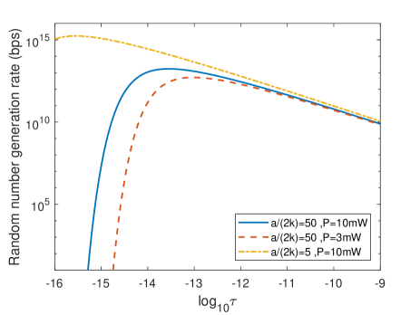
Figure 4: The lower bound of random number generation rate with different resolutions of the ADC and different local oscillator intensities.

IV Conclusion and Outlook

In this work, we investigate the randomness quantification in shot-noise driven QRNG based on coherent detection. By characterizing the local oscillator in a quantum way, we find the outcome of homodyne detection is actually an infinite dimensional discrete variable rather than a continuous one, whose randomness is quantified by infinite-dimensional coherence. Considering experimental parameters, we calculate practical upper and lower bounds of the randomness generation rate.

As a beginning, our work provides a new point of view on the coherent detection. For future work, we may take more practical issues into consideration, such as electronic noises, bandwidth of photodetectors, and more important, intensity fluctuations of the local oscillator and input state. These intensity fluctuations will make the coherent states in our model become mixed, which will be exploited by the adversary to extract side information. The randomness quantification in this case is quite challenging.

Moreover, our technique for randomness quantification in coherent detection is applicable to other scenarios that a similar setup is used. One example is phase fluctuation extracting randomness from spontaneous emission. The bottleneck lies in how to characterize the entropy source, i.e., a coherent light carrying a random phase introduced by spontaneous emission.

Another key example is the continuous-variable quantum key distribution (CV-QKD) systems where a Gaussian-modulated coherent state by Alice is measured by a homodyne receiver at Bob’s end Grosshans and Grangier (2002). The key rate calculations will then involve estimating the mutual information between Alice and Bob and upper bounding the Holevo information between Alice/Bob and Eve (depending on whether direct/reverse reconciliation is in use) Devetak and Winter (2005). The common assumption in such calculations is that of treating the local oscillator classically, or, equivalently, assuming that the local oscillator is of infinitely large intensity. If one wants to account for the effect of having a finite-power oscillator, then one can use the techniques we developed in this work, and the security analysis may fall in to the same framework of discrete variable quantum key distribution (DV-QKD).

Appendix A Classical model of homodyne detection

Homodyne detection settings, made up of a beam splitter and two photodetectors, have two inputs: a local oscillator (LO), which can be described as a strong coherent state $\left|\alpha_{LO}\right\rangle$, and a signal state $\rho$. After a transformation from photon intensity to current by the photodetector, a subtraction of current is performed to mitigate the classical electronic noise.

The output in the homodyne detection is given by the operator,

$$\delta\hat{i}=\hat{i}_{1}-\hat{i}_{2}=k(\hat{a}^{\dagger}_{LO}\hat{a}+\hat{a}^{{\dagger}}\hat{a}_{LO}).$$ (18)

where $\hat{a}$ and $\hat{a}_{LO}$ are annihilation operators of the input optical modes. And for a photodetector, we make an assumption that the current is proportional to photon number and the coefficient is $k$. Note that all the calculation above is in the Heisenberg picture. Hence the expectation value of $\delta\hat{i}$ is $Tr(\delta\hat{i}\rho\otimes\mbox{$\left|\alpha_{LO}\right\rangle$}\mbox{$\left\langle\alpha_{LO}\right|$})$ and the variance is $Tr(\delta\hat{i}^{2}\rho\otimes\mbox{$\left|\alpha_{LO}\right\rangle$}\mbox{$\left\langle\alpha_{LO}\right|$})-(Tr(\delta\hat{i}\rho\otimes\mbox{$\left|\alpha_{LO}\right\rangle$}\mbox{$\left\langle\alpha_{LO}\right|$}))^{2}$. When the intensity of the LO is strong enough, the homodyne detection can be regarded as a measurement of quadratures as an approximation. Considering the phase of the LO, $\alpha_{LO}=|\alpha_{LO}|e^{i\phi}$, the expectation and variance can be rewritten as

$$\langle\delta\hat{i}\rangle=2k|\alpha_{LO}|\mathrm{tr}(\hat{x}(\phi)\rho)$$ (19)

$$\langle\delta\hat{i}^{2}\rangle-\langle\delta\hat{i}\rangle^{2}$$

$$=4k^{2}|\alpha_{LO}|^{2}[\mathrm{tr}(\hat{x}^{2}(\phi)\rho)-(\mathrm{tr}(\hat{x}(\phi)\rho))^{2}]+k^{2}\mathrm{tr}(\hat{a}^{\dagger}\hat{a}\rho),$$

where $\hat{x}(\phi)=(\hat{a}e^{-i\phi}+\hat{a}^{{\dagger}}e^{i\phi})/2$ is a quadrature of the signal state depending on $\phi$. When $\phi=0$ or $\pi/2$, it corresponds to $\hat{x}=(\hat{a}+\hat{a}^{\dagger})/2$ or $\hat{p}=(\hat{a}-\hat{a}^{\dagger})/2$ quadrature respectively, that is, the quantity measured by the homodyne detection depends on the phase $\phi$ of the LO.

Appendix B Quantum min-entropy can reduce to its classical counterpart

In this section we prove the quantum min-entropy will reduce to the classical min-entropy function when the adversary has no side information of the measurement outcomes, i.e, $\rho_{A}$ is a pure state. We begin with Eq. (8)

$$S_{min}(A^{\prime}|E) =\max_{\sigma_{E}}\sup\{\lambda\in\mathcal{R}:\rho_{A^{\prime}E}\leq 2^{-\lambda}I_{A}\otimes\sigma_{E}\}$$ (20)

$$=\min_{\sigma_{E}}\inf\{p\in\mathcal{R}:pI_{A}\otimes\sigma_{E}\geq\rho_{A^{\prime}E}\}$$

$$=\min_{\sigma_{E}}\inf\{p\in\mathcal{R}:pI_{A}\otimes\sigma_{E}\geq\rho_{A^{\prime}}\otimes\rho_{E}\}$$

where $p=2^{-\lambda}$, the last equation is because $\rho_{A}$ is pure and after the measurement on $A$, $\rho_{A^{\prime}E}$ is also a product state. Now we need to let $p$ as small as possible such that $pI_{A}\otimes\sigma_{E}\geq\rho_{A^{\prime}}\otimes\rho_{E}$ which can be rewritten as

$$\sum_{i}\mbox{$\left|i\right\rangle$}\mbox{$\left\langle i\right|$}\otimes(p\sigma_{E}-p_{i}\rho_{E})$$ (21)

We only need to consider $p\sigma_{E}-p_{i}\rho_{E}\geq 0$. Note that $\rho_{E}$ is a pure state with only one non-zero eigenvalue $\eta=1$ in its spectrum. In order to let $p$ as small as possible, the best choice is to let $\sigma_{E}$ also be a pure state $\sigma_{E}=\rho_{E}$ and $p\geq p_{i}$. Consider all decomposition components in Eq. (21), $p=\max_{i}p_{i}$ and $\lambda=-\log_{2}(\max_{i}p_{i})$ which is just the classical min-entropy function.

References

- Bennett and Brassard (1984) C. H. Bennett and G. Brassard, in Proceedings of the IEEE International Conference on Computers, Systems and Signal Processing (IEEE Press, New York, 1984) pp. 175–179.
- Ekert (1991) A. K. Ekert, Phys. Rev. Lett. 67, 661 (1991).
- Ma et al. (2016) X. Ma, X. Yuan, Z. Cao, B. Qi, and Z. Zhang, npj Quantum Information 2, 16021 (2016), review Article.
- Herrero-Collantes and Garcia-Escartin (2017) M. Herrero-Collantes and J. C. Garcia-Escartin, Rev. Mod. Phys. 89, 015004 (2017).
- Grosshans and Grangier (2002) F. Grosshans and P. Grangier, Phys. Rev. Lett. 88, 057902 (2002).
- Grosshans et al. (2003) F. Grosshans, G. Van Assche, J. Wenger, R. Brouri, N. J. Cerf, and P. Grangier, Nature 421, 238 (2003).
- Gabriel et al. (2010) C. Gabriel, C. Wittmann, D. Sych, R. Dong, W. Mauerer, U. L. Andersen, C. Marquardt, and G. Leuchs, Nature Photonics 4, 711 (2010).
- Shen et al. (2010) Y. Shen, L. Tian, and H. Zou, Physical Review A 81, 063814 (2010).
- Symul et al. (2011) T. Symul, S. Assad, and P. K. Lam, Applied Physics Letters 98, 231103 (2011).
- Jofre et al. (2011) M. Jofre, M. Curty, F. Steinlechner, G. Anzolin, J. Torres, M. Mitchell, and V. Pruneri, Optics express 19, 20665 (2011).
- Shi et al. (2016) Y. Shi, B. Chng, and C. Kurtsiefer, Applied Physics Letters 109 (2016), http://dx.doi.org/10.1063/1.4959887.
- Marangon et al. (2017) D. G. Marangon, G. Vallone, and P. Villoresi, Phys. Rev. Lett. 118, 060503 (2017).
- Xu et al. (2017) B. Xu, Z. Li, J. Yang, S. Wei, Q. Su, W. Huang, Y. Zhang, and H. Guo, arXiv preprint arXiv:1709.00685 (2017).
- Haylock et al. (2018) B. Haylock, D. Peace, F. Lenzini, C. Weedbrook, and M. Lobino, arXiv preprint arXiv:1801.06926 (2018).
- Guo et al. (2018) X. Guo, R. Liu, P. Li, C. Cheng, M. Wu, and Y. Guo, arXiv preprint arXiv:1805.10506 (2018).
- Avesani et al. (2018) M. Avesani, D. G. Marangon, G. Vallone, and P. Villoresi, arXiv preprint arXiv:1801.04139 (2018).
- Zheng et al. (2018) Z. Zheng, Y.-C. Zhang, W. Huang, S. Yu, and H. Guo, arXiv preprint arXiv:1805.08935 (2018).
- Fürst et al. (2010) H. Fürst, H. Weier, S. Nauerth, D. G. Marangon, C. Kurtsiefer, and H. Weinfurter, Optics express 18, 13029 (2010).
- Yan et al. (2014) Q. Yan, B. Zhao, Q. Liao, and N. Zhou, Review of Scientific Instruments 85, 103116 (2014).
- Qi et al. (2010) B. Qi, Y.-M. Chi, H.-K. Lo, and L. Qian, Optics letters 35, 312 (2010).
- Xu et al. (2012) F. Xu, B. Qi, X. Ma, H. Xu, H. Zheng, and H.-K. Lo, Optics express 20, 12366 (2012).
- Nie et al. (2014) Y.-Q. Nie, H.-F. Zhang, Z. Zhang, J. Wang, X. Ma, J. Zhang, and J.-W. Pan, Applied Physics Letters 104, 051110 (2014).
- Nie et al. (2015) Y.-Q. Nie, L. Huang, Y. Liu, F. Payne, J. Zhang, and J.-W. Pan, Review of Scientific Instruments 86, 063105 (2015).
- Zhang et al. (2016a) X.-G. Zhang, Y.-Q. Nie, H. Zhou, H. Liang, X. Ma, J. Zhang, and J.-W. Pan, Review of Scientific Instruments 87, 076102 (2016a).
- Yang et al. (2016) J. Yang, J. Liu, Q. Su, Z. Li, F. Fan, B. Xu, and H. Guo, Optics Express 24, 27475 (2016).
- Sun and Xu (2017) S.-H. Sun and F. Xu, Phys. Rev. A 96, 062314 (2017).
- Jennewein et al. (2000) T. Jennewein, U. Achleitner, G. Weihs, H. Weinfurter, and A. Zeilinger, Review of Scientific Instruments 71, 1675 (2000).
- Stefanov et al. (2000) A. Stefanov, N. Gisin, O. Guinnard, L. Guinnard, and H. Zbinden, Journal of Modern Optics 47, 595 (2000).
- Cao et al. (2015) Z. Cao, H. Zhou, and X. Ma, New Journal of Physics 17, 125011 (2015).
- Cao et al. (2016) Z. Cao, H. Zhou, X. Yuan, and X. Ma, Phys. Rev. X 6, 011020 (2016).
- Ma et al. (2013) X. Ma, F. Xu, H. Xu, X. Tan, B. Qi, and H.-K. Lo, Phys. Rev. A 87, 062327 (2013).
- Zhou et al. (2015) H. Zhou, X. Yuan, and X. Ma, Phys. Rev. A 91, 062316 (2015).
- Baumgratz et al. (2014) T. Baumgratz, M. Cramer, and M. Plenio, Physical review letters 113, 140401 (2014).
- Yuan et al. (2015) X. Yuan, H. Zhou, Z. Cao, and X. Ma, Physical Review A 92, 022124 (2015).
- Yuan et al. (2016) X. Yuan, Q. Zhao, D. Girolami, and X. Ma, arXiv preprint arXiv:1605.07818 (2016).
- Zhang et al. (2016b) Y.-R. Zhang, L.-H. Shao, Y. Li, and H. Fan, Physical Review A 93, 012334 (2016b).
- Skellam (1945) J. G. Skellam, Journal of the Royal Statistical Society. Series A (General) 109, 296 (1945).
- Abramowitz et al. (1966) M. Abramowitz, I. A. Stegun, et al., Applied mathematics series 55, 62 (1966).
- Tomamichel (2012) M. Tomamichel, arXiv preprint arXiv:1203.2142 (2012).
- Nyquist (1928) H. Nyquist, Transactions of the American Institute of Electrical Engineers 47, 617 (1928).
- Shannon (1949) C. E. Shannon, Bell Labs Technical Journal 28, 656 (1949).
- Devetak and Winter (2005) I. Devetak and A. Winter, Proceedings of the Royal Society of London A: Mathematical, Physical and Engineering Sciences 461, 207 (2005).