Many-body effects in twisted bilayer graphene at low twist angles

Abstract

We study the zero-temperature many-body properties of twisted bilayer graphene with a twist angle equal to the so-called ‘first magic angle’. The system low-energy single-electron spectrum consists of four (eight, if spin label is accounted) weakly-dispersing partially degenerate bands, each band accommodating one electron per Moiré cell per spin projection. This weak dispersion makes electrons particularly susceptible to the effects of interactions. Introducing several excitonic order parameters with spin-density-wave-like structure, we demonstrate that (i) the band degeneracy is partially lifted by the interaction, and (ii) the details of the low-energy spectrum becomes doping-dependent. For example, at or near the undoped state, interactions separate the eight bands into two quartets (one quartet is almost filled, the other is almost empty), while for two electrons per Moiré cell, the quartets are pulled apart, and doublets emerge. When the doping is equal to one or three electrons per cell, the doublets split into singlets. Hole doping produces similar effects. As a result, electronic properties (e.g., the density of states at the Fermi energy) demonstrate oscillating dependence on the doping concentration. This allows us to reproduce qualitatively the behavior of the conductance observed recently in experiments [Cao et al., Nature 556, 80 (2018)]. Near half-filling, the electronic spectrum loses hexagonal symmetry indicating the appearance of a many-body nematic state.

I Introduction

The search for broken-symmetry phases in graphene bilayer systems remains an active research area Rozhkov et al. (2016). Theorists have studied a variety of possibilities, such as antiferromagnetism Kharitonov (2012); Akzyanov et al. (2014); de la Peña et al. (2014); Lemonik et al. (2012); Nilsson et al. (2006); Sboychakov et al. (2013a, b); Lang et al. (2012); Rakhmanov et al. (2012), superconductivity McChesney et al. (2010); Kagan et al. (2015, 2014); González et al. (2001); Alidoust et al. (2019), excitons Lozovik and Sokolik (2008, 2009); Akzyanov et al. (2014); Sboychakov et al. (2018), as well as more exotic states Lemonik et al. (2012); Zhang and MacDonald (2012). Unfortunately, experimentally, the broken symmetry phases are rare celebrities in graphene systems, except, perhaps, AB bilayer graphene, for which numerous experiments Freitag et al. (2013); Maher et al. (2013); Bao et al. (2012); van Elferen et al. (2012); Freitag et al. (2012); Velasco Jr. et al. (2012) provide evidence of low-temperature non-superconducting order. It appears, however, that the situation in this field has changed: in recent experiments Cao et al. (2018a, b) both superconductivity and many-body insulating states were detected in doped samples of twisted bilayer graphene (TBLG) whose twist angles $\theta$ are close to the so-called ‘first magic angle’ $\theta_{c}\approx 1.1^{\circ}$. The dependence of the conductance $\sigma$, as a function of doping $n$, showed several pronounced minima: at $n=0$ (undoped state), at $n=\pm n_{s}/2$, and at $n=\pm n_{s}$ (the doping level $n=n_{s}$ corresponds to one electron per spin projection per layer per supercell, or, equivalently, four electrons per supercell). In some samples, additional minima were observed at ext (a) $n=\pm 3n_{s}/4$, and at wea $n=n_{s}/4$. The purpose of this paper is to offer a theoretical explanation to these remarkable findings.

Our reasoning relies on the peculiar band structure of TBLG at small twist angles: for $\theta\leq\theta_{c}$, the low-energy single-electron spectrum is dominated by four (eight, if spin degeneracy is accounted) bands with almost no dispersion ext (b), and the Fermi surface is present even at zero doping Sboychakov et al. (2015) (provided that the interaction effects are neglected). The single-electron density of states (DOS) of these bands offers a simple explanation Cao et al. (2018a) for the conductance minima at $n=\pm n_{s}$. As for the minima in the interval $-n_{s}<n<n_{s}$, such single-body reasoning fails to explain them, and a many-body formalism is necessary. Indeed, the flatness and degeneracy of the low-energy bands make them particularly susceptible to the interaction effects. To account for the latter, we use a mean-field approach. A simple single-site spin-density wave (SDW) order parameter is sufficient to reproduce the minimum at $n=0$: in energy space, such an order parameter splits the eight bands into two quartets, one quartet is almost filled, the other is almost empty, with drastically reduced DOS at the Fermi level. To explain the behavior of $\sigma(n)$ at other $n$’s, the quartets must be split further (into doublets and singlets), which requires more complex SDW order parameters. The resultant formalism captures qualitatively the dependence of $\sigma$ versus doping reported in Ref. Cao et al., 2018a. In addition, our calculations demonstrate that for sufficiently large doping the so-called electronic nematicity may be stabilized.

The paper is organized as follows. The basic facts about the TBLG geometry are outlined in Sec. II. The studied model is formulated in Sec. III. The mean field approximation is applied to the model in Sec. IV. Section V is dedicated to the discussions of the presented results, while the conclusions are formulated in Sec. VI.

II Geometry of twisted bilayer graphene

To introduce the notation, let us start with a brief review of basic TBLG geometrical facts. More details can be found in Refs. Lopes dos Santos et al., 2012; Mele, 2012; Rozhkov et al., 2016. A graphene monolayer has a hexagonal crystal structure consisting of two triangular sublattices ${\cal A}$ and ${\cal B}$. The coordinates of atoms in layer $1$ on sublattice ${\cal A}$ are

$$\mathbf{r}_{\mathbf{n}}^{1{\cal A}}=\mathbf{r}_{\mathbf{n}}^{1}\equiv n\mathbf{a}_{1}+m\mathbf{a}_{2},$$ (1)

where $\mathbf{n}=(n,\,m)$ is an integer-valued vector,

$$\mathbf{a}_{1,2}=a(\sqrt{3},\mp 1)/2$$ (2)

are the primitive vectors, $a=2.46$ Å is the lattice constant of graphene. The coordinates of atoms on sublattice ${\cal B}$ are

$$\mathbf{r}_{\mathbf{n}}^{1{\cal B}}=\mathbf{r}_{\mathbf{n}}^{1}+\bm{\delta},$$ (3)

where

$$\bm{\delta}=a(1/\sqrt{3},0).$$ (4)

Atoms in layer $2$ are located at

$$\mathbf{r}_{\mathbf{n}}^{2{\cal B}}=\mathbf{r}_{\mathbf{n}}^{2}\equiv d\mathbf{e}_{z}+n\mathbf{a}_{1}^{\prime}+m\mathbf{a}_{2}^{\prime},\quad\mathbf{r}_{\mathbf{n}}^{2{\cal A}}=\mathbf{r}_{\mathbf{n}}^{2}-\bm{\delta}^{\prime},$$ (5)

where $\mathbf{a}_{1,2}^{\prime}$ and $\bm{\delta}^{\prime}$ are the vectors $\mathbf{a}_{1,2}$ and $\bm{\delta}$, rotated by an angle $\theta$. The unit vector along the $z$-axis is $\mathbf{e}_{z}$, the inter-layer distance is $d=3.35$ Å. The limiting case $\theta=0$ corresponds to the AB stacking.

If the twist angle satisfies

$$\cos\theta=\frac{3m_{0}^{2}+3m_{0}r+r^{2}/2}{3m_{0}^{2}+3m_{0}r+r^{2}},$$ (6)

where $m_{0}$ and $r$ are co-prime positive integers, a superstructure emerges, and a TBLG sample splits into a periodic lattice of finite supercells. The number of graphene unit cells inside a supercell is

$$N_{\rm sc}=(3m_{0}^{2}+3m_{0}r+r^{2})/g$$ (7)

per layer, where $g=1$ if $r\neq 3n$, or $g=3$ otherwise.

The reciprocal lattice primitive vectors for the layer 1 are denoted by $\mathbf{b}_{1,2}$, for layer 2 they are $\mathbf{b}_{1,2}^{\prime}$. In layer 1 we have

$$\mathbf{b}_{1,2}=(2\pi/\sqrt{3},\mp 2\pi)/a,$$ (8)

while $\mathbf{b}_{1,2}^{\prime}$ are connected to $\mathbf{b}_{1,2}$ by rotating on angle $\theta$.

When the superlattice is present, the primitive reciprocal vectors for the superlattice can be defined. We denote them as $\bm{{\cal G}}_{1,2}$. For these vectors, the following identities in the reciprocal space are valid:

$$\mathbf{b}_{1}^{\prime}=\mathbf{b}_{1}+r(\bm{{\cal G}}_{1}+\bm{{\cal G}}_{2}),\quad\mathbf{b}_{2}^{\prime}=\mathbf{b}_{2}-r\bm{{\cal G}}_{1},$$ (9)

if $r\neq 3n$, or

$$\mathbf{b}_{1}^{\prime}=\mathbf{b}_{1}+r(\bm{{\cal G}}_{1}+2\bm{{\cal G}}_{2})/3,$$ (10)

$$\mathbf{b}_{2}^{\prime}=\mathbf{b}_{2}-r(2\bm{{\cal G}}_{1}+\bm{{\cal G}}_{2})/3,$$ (11)

otherwise. The Brillouin zone of the superlattice is hexagonal-shaped. It can be obtained by $N_{\rm sc}$-times folding of the Brillouin zone of the layer $1$ or $2$. Two non-equivalent corners of the reduced Brillouin zone, $\mathbf{K}_{1}$ and $\mathbf{K}_{2}$, can be expressed via vectors $\bm{{\cal G}}_{1,2}$ as

$$\mathbf{K}_{1}=(\bm{{\cal G}}_{1}+2\bm{{\cal G}}_{2})/3,\quad\mathbf{K}_{2}=(2\bm{{\cal G}}_{1}+\bm{{\cal G}}_{2})/3.$$ (12)

III Model Hamiltonian

III.1 Single-electron term

We investigate the tight-binding model for $p_{z}$ electrons in the TBLG at small doping $n$. The Hamiltonian is

$${\hat{H}}={\hat{H}}_{0}+{\hat{H}}_{\rm int},$$ (13)

where ${\hat{H}}_{\rm int}$ is the electron-electron interaction, and a single-electron term equals to

$${\hat{H}}_{0}\!=\!\sum_{{i\mathbf{n}j\mathbf{m}\atop ss^{\prime}\sigma}}\!t(\mathbf{r}_{\mathbf{n}}^{is};\mathbf{r}_{\mathbf{m}}^{js^{\prime}}){\hat{d}}^{{\dagger}}_{\mathbf{n}is\sigma}{\hat{d}}^{\phantom{{\dagger}}}_{\mathbf{m}js^{\prime}\sigma}.$$ (14)

In this expression ${\hat{d}}^{{\dagger}}_{\mathbf{n}is\sigma}$ (${\hat{d}}^{\phantom{{\dagger}}}_{\mathbf{n}is\sigma}$) are the creation (annihilation) operators of the electron with spin $\sigma$ at the unit cell $\mathbf{n}$ in the layer $i$ ($=1,2$) in the sublattice $s$ ($={\cal A,B}$). For intra-layer hopping, only the nearest-neighbor term is included. Its value is $t=-2.57$ eV. The inter-layer hoppings are parameterized as described in Refs. Trambly de Laissardière et al., 2012, 2010, with the largest inter-layer hopping amplitude being equal to $t_{0}=0.4$ eV.

Switching to the momentum representation, one can introduce new single-particle operators

$${\hat{d}}^{\phantom{{\dagger}}}_{\mathbf{pG}is\sigma}={\cal N}^{-1/2}\sum_{\mathbf{n}}e^{-i(\mathbf{p}+\mathbf{G})\mathbf{r}_{\mathbf{n}}^{i}}{\hat{d}}_{\mathbf{n}is\sigma}.$$ (15)

Here ${\cal N}$ is the number of graphene unit cells in the sample in one layer, the momentum $\mathbf{p}$ lies in the first Brillouin zone of the superlattice, while $\mathbf{G}=m_{1}\bm{{\cal G}}_{1}+m_{2}\bm{{\cal G}}_{2}$ is the reciprocal vector of the superlattice lying in the first Brillouin zone of the $i$th layer. The number of such vectors $\mathbf{G}$ is equal to $N_{\rm sc}$ for each graphene layer. Thus, ${\hat{H}}_{0}$ becomes

$${\hat{H}}_{0}\!=\!\!\!\sum_{\mathbf{p}\mathbf{G}_{1,2}}\sum_{ijss^{\prime}\sigma}\!\tilde{t}_{ij}^{ss^{\prime}}(\mathbf{p}\!+\!\mathbf{G}_{1};\mathbf{G}_{1}\!-\!\mathbf{G}_{2}){\hat{d}}^{{\dagger}}_{\mathbf{pG}_{1}is\sigma}{\hat{d}}^{\phantom{{\dagger}}}_{\mathbf{pG}_{2}js^{\prime}\sigma},\$$ (16)

where the hopping amplitudes in momentum space are

$$\tilde{t}_{ij}^{ss^{\prime}}(\mathbf{k};\mathbf{G})\!=\!\frac{1}{N_{\rm sc}}\!\mathop{{\sum}^{\prime}}_{\mathbf{nm}}\!e^{-i\mathbf{k}(\mathbf{r}_{\mathbf{n}}^{i}-\mathbf{r}_{\mathbf{m}}^{j})}e^{-i\mathbf{G}\mathbf{r}_{\mathbf{m}}^{j}}\,\,t(\mathbf{r}_{\mathbf{n}}^{is};\mathbf{r}_{\mathbf{m}}^{js^{\prime}})\,.$$ (17)

The summation symbol with prime $\sum^{\prime}_{\bf nm}$ implies that $\mathbf{m}$ runs over sites inside the zeroth supercell, while $\mathbf{n}$ runs over all sites in the sample.

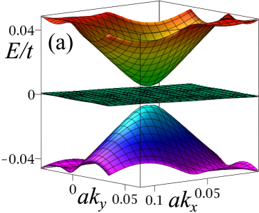
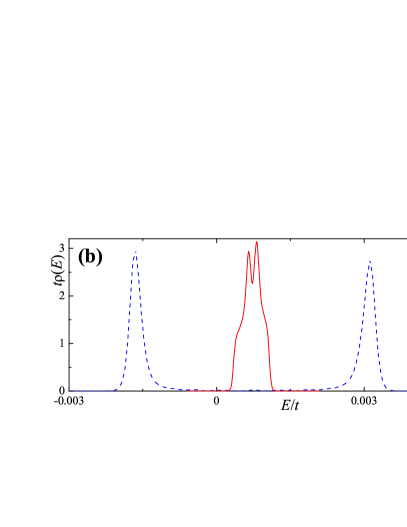
Figure 1: (a) Single-particle low-energy band structure (interaction effects are neglected here) inside the superlattice Brillouin zone calculated for the first magic angle $\theta=\theta_{c}$. (b) Low-energy DOS $\rho(E)$ corresponding to the band structure shown above (solid curve) and for the band structure modified by interaction (dashed curve), see Fig. 2(a) and text below.

Single-electron energies $E_{\mathbf{p}}^{S}$ and corresponding eigenvectors $\Phi^{S}_{\mathbf{pG}is}$ (here $S=1,\,2,\,\dots,\,4N_{\rm sc}$ enumerates all $4N_{\rm sc}$ spin-degenerate bands of the TBLG) are found by numerical diagonalization of Eq. (16). The spectrum of (16) is well-studied. Its properties at small and large $\theta$ differ qualitatively. When $\theta>\theta_{c}$ (for the hopping parameters used here $\theta_{c}\approx 1.08^{\circ}$), the low-energy spectrum is Dirac-like. If $\theta\leq\theta_{c}$, the system acquires a Fermi surface, which is formed by four (eight, if spin degeneracy is accounted) almost-flat partially degenerate bands at low energy ext (b). In Fig. 1 (a) the spectrum of this type is plotted for ‘the first magic angle’ $\theta=\theta_{c}$. We see that higher-energy electron and hole bands with pronounced dispersion are separated from each other by sheets of almost-flat bands. This peculiar spectrum structure is the origin of the many-body physics discussed below.

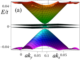
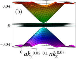
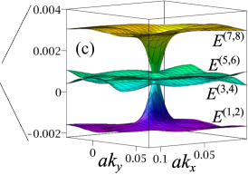
Figure 2: (a) Charge neutrality band structure modified by the interaction (20). The eight bands are split into two quartets (individual bands are indiscernible due to small energy separations between the bands of the same quartet). (b) When $n=n_{s}/2$, the order parameters $A$ split the two-quartet structure [panel (a)] into the doublet-quartet-doublet structure. (c) Fine structure of the low-energy bands shown in panel (b). The energy bands are labeled by $E^{(\alpha)}$, $\alpha=1\ldots 8$.

To characterize this non-interacting spectrum more thoroughly, it is instructive to calculate the low-energy DOS

$$\rho(E)=2\sum_{S}\int\frac{d^{2}{\bf p}}{v_{\rm SBZ}}\delta(E^{S}_{\bf p}-E),$$ (18)

where the integral is taken over the superlattice Brillouin zone, whose area is denoted by $v_{\rm SBZ}$. The DOS is plotted in Fig. 1 (b). It has a double peak structure, with the total spectral weight corresponding to eight electrons per a Moiré cell. The DOS remains non-zero for any doping in the interval $|n|<n_{s}$, as expected for a system with a Fermi surface Sboychakov et al. (2015). The Fermi energy for the undoped state $n=0$ corresponds to the minimum on the DOS plot. The overall structure of the DOS plot and its width

$$W\sim 2\,{\rm meV}$$ (19)

are consistent with Fig. 1d of Ref. Cao et al., 2018b.

Numerical calculations demonstrate that the flat bands are separated from the rest of the spectrum by two gaps, both of the order of 15 meV, in qualitative agreement with other computational and experimental Cao et al. (2018b); Carr et al. (2019) results.

III.2 Interactions term

To model experimental conditions Cao et al. (2018a, b), we study the many-body effects for $\theta=\theta_{c}$. As a starting point of our analysis, we model ${\hat{H}}_{\rm int}$ using the Hubbard interaction

$${\hat{H}}_{\rm int}\!=\!\frac{U}{2}\!\!\sum_{{\mathbf{n}is\sigma}}\!\!{\hat{d}}^{{\dagger}}_{\mathbf{n}is\sigma}{\hat{d}}^{\phantom{{\dagger}}}_{\mathbf{n}is\sigma}{\hat{d}}^{{\dagger}}_{\mathbf{n}is\bar{\sigma}}{\hat{d}}^{\phantom{{\dagger}}}_{\mathbf{n}is\bar{\sigma}},$$ (20)

$$U=2t<U_{c}^{\rm MF}\,.$$ (21)

Here the notation $\bar{\sigma}$ means ‘not $\sigma$’, and

$$U_{c}^{\rm MF}\approx 2.23t$$ (22)

is the critical strength for a single-layer graphene transition into a mean-field antiferromagnetic state Sorella and Tosatti (1992). The choice (21) implies that the interaction in our model is strong; yet, not strong enough to cause a single-layer many-body instability, at least in the mean-field framework. In other words, the presence of the second layer is a necessary prerequisite for a mean-field transition.

IV Mean-field calculations

IV.1 Single-site order parameter

To account for the interaction (20) at the mean-field level, we must choose a suitable order parameter. First, let us define Gonzalez-Arraga et al. (2017); Rakhmanov et al. (2012); Sboychakov et al. (2013a, b); Akzyanov et al. (2014) the single-site magnetization

$$\eta_{\mathbf{m}is\sigma}=\langle{\hat{d}}^{{\dagger}}_{\mathbf{m}is\sigma}{\hat{d}}^{\phantom{{\dagger}}}_{\mathbf{m}is\bar{\sigma}}\rangle,$$ (23)

where $\langle\ldots\rangle$ denotes the averaging with respect to the mean-field ground state. We will assume that the anomalous average $\eta_{\mathbf{m}is\sigma}$, as a function of position $\mathbf{m}$, has the same period as the superlattice. That is, only the spin-rotational symmetry is broken, while the superlattice translation symmetry is preserved (the spin texture has the same periodicity as the superlattice). Using the $\eta$’s we decouple $H_{\rm int}$, to obtain the mean-field interaction

$${\hat{H}}_{\rm int}^{\rm MF}\!=\!\sum_{\mathbf{n}is\sigma}\left[-\Delta_{\mathbf{n}is\sigma}^{\vphantom{\dagger}}{\hat{d}}^{{\dagger}}_{\mathbf{n}is\bar{\sigma}}{\hat{d}}^{\phantom{{\dagger}}}_{\mathbf{n}is\sigma}+\frac{\left|\Delta_{\mathbf{n}is\sigma}\right|^{2}}{2U}\right].$$ (24)

Here

$$\Delta_{\mathbf{n}is\sigma}=U\eta_{\mathbf{n}is\sigma}$$ (25)

is the order parameter. Finding the self-consistent value of $\Delta_{\mathbf{n}is\sigma}$, we can determine the low-energy band structure of our model, modified by the interaction (20). Figure 2 (a) presents the results of such calculations for $n=0$. The order parameter $\Delta_{\mathbf{n}is\sigma}$ lifts the degeneracy of the low-energy spectrum, splitting the eight energy bands into two quartets: four bands are pushed above the Fermi level $\varepsilon_{\rm F}$, and four other bands sink below $\varepsilon_{\rm F}$. Each quartet appears as a peak in the DOS plot in Fig. 1(b). The peaks are separated by

$$E_{g}\approx 4.5\times 10^{-3}t\approx 12\,{\rm meV}.$$ (26)

Although most of the electronic states are pushed away from the Fermi energy $\varepsilon_{\rm F}$, near the $\Gamma$ point the quartets cross the Fermi energy level, forming a Fermi surface, and generating a small but finite $\rho(\varepsilon_{\rm F})$. Thus, consistent with experiments Cao et al. (2018a), the undoped state is metallic.

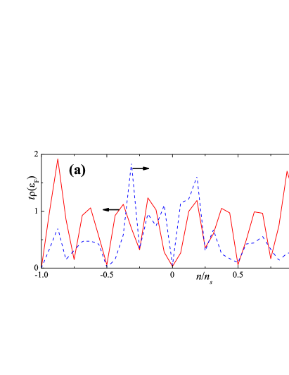
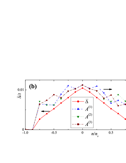
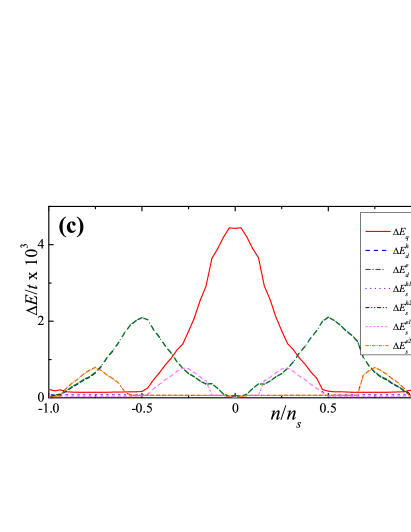
Figure 3: (a) The DOS at Fermi energy $\rho(\varepsilon_{\rm F})$, shown by solid curve, and the conductance $\sigma$, shown by dashed curve, as functions of doping. (b) Dependence of $\bar{\Delta}$ and $A^{(\ell)}$, defined by Eqs. (43-46), on doping $n$. For $|n|\leq n_{s}/8$, we find $A^{(1)}=A^{(2)}=A^{(3)}$. When $|n|>n_{s}/8$, the latter identity is violated, indicating the emergence of the so-called electronic nematicity. (c) The dependence of band separation parameters as functions of $n$. The curves for $\Delta E_{\rm d}^{\rm e}$ and $\Delta E_{\rm d}^{\rm h}$ coincide. The same is true for $\Delta E_{\rm s}^{\rm h1}$ and $\Delta E_{\rm s}^{\rm e1}$, as well as for $\Delta E_{\rm s}^{\rm h2}$ and $\Delta E_{\rm s}^{\rm e2}$.

IV.2 Two-site order parameter

However, our mean-field calculations show that the order parameter (24) is sufficient to describe the conductivity suppression near the charge neutrality point only. Yet, in the range $0<|n|<n_{s}$ the mean-field theory based on purely single-site order parameter, Eq. (23), predicts quite featureless evolution of the system properties. For our goals, the most important shortcoming of the purely single-site order parameter is its inability to split the quartets of the bands further, into doublets, and single bands.

To appreciate the importance of the latter prerequisite, consider the following reasoning. Experimentally, doping levels $n=\pm n_{s}/2$ are special for the system demonstrates drastic depletion of the conductivity. On the theory side, doping $n=n_{s}/2$ (doping $n=-n_{s}/2$) corresponds to two additional electrons (two additional holes) per supercell, or, equivalently, it requires complete filling (complete draining) of exactly two bands of the upper (lower) quartet. Therefore, an insulating or poorly conducting state at $n=\pm n_{s}/2$ requires the separation of the quartet of bands into two doublets, one of which is filled, the other is empty.

Our numerical study shows that, to generate the desired splitting, the interaction Hamiltonian, besides the Hubbard term (20), must include the term describing the (Coulomb) interaction of electrons on neighboring sites:

$$H^{C}_{\rm int}=\frac{1}{2}\!\!\!\sum_{{\bf nm}ij\atop ss^{\prime}\sigma\sigma^{\prime}}\!\!\!V(\mathbf{r}^{is}_{\mathbf{n}}-\mathbf{r}^{js^{\prime}}_{\mathbf{m}}){\hat{d}}^{{\dagger}}_{\mathbf{n}is\sigma}{\hat{d}}^{\phantom{{\dagger}}}_{\mathbf{n}is\sigma}{\hat{d}}^{{\dagger}}_{\mathbf{m}js^{\prime}\sigma^{\prime}}{\hat{d}}^{\phantom{{\dagger}}}_{\mathbf{m}js^{\prime}\sigma^{\prime}}.\quad$$ (27)

This interaction can be decoupled by the following excitonic order parameter:

$$A^{\mathbf{n}is}_{\mathbf{m}js^{\prime};\sigma}=V(\mathbf{r}^{is}_{\mathbf{n}}-\mathbf{r}^{js^{\prime}}_{\mathbf{m}})\langle{\hat{d}}^{{\dagger}}_{\mathbf{n}is\sigma}{\hat{d}}^{\phantom{{\dagger}}}_{\mathbf{m}js^{\prime}\bar{\sigma}}\rangle.$$ (28)

The mean-field version of the interaction (27) is

$${\hat{H}}_{\rm int}^{C,\,{\rm MF}}=-\frac{1}{2}\sum_{\mathbf{nm}ij\atop ss^{\prime}\sigma}\!\!\left[A^{\mathbf{n}is}_{\mathbf{m}js^{\prime};\sigma}{\hat{d}}^{{\dagger}}_{\mathbf{m}js^{\prime}\bar{\sigma}}{\hat{d}}^{\vphantom{{\dagger}}}_{\mathbf{n}is\sigma}+{\rm H.c.}\right]$$

$$+\frac{1}{2}\sum_{\mathbf{nm}ij\atop ss^{\prime}\sigma}\!\frac{\left|A^{\mathbf{n}is}_{\mathbf{m}js^{\prime};\sigma}\right|^{2}}{V(\mathbf{r}^{is}_{\mathbf{n}}-\mathbf{r}^{js^{\prime}}_{\mathbf{m}})}\,.$$ (29)

For calculations we assume that order parameter $A^{\mathbf{n}is}_{\mathbf{m}js^{\prime};\sigma}$ is non-zero only when sites $\mathbf{r}_{\mathbf{n}}^{is}$ and $\mathbf{r}_{\mathbf{m}}^{js^{\prime}}$ are sufficiently close. Namely, if the hopping amplitude connecting $\mathbf{r}_{\mathbf{n}}^{is}$ and $\mathbf{r}_{\mathbf{m}}^{js^{\prime}}$ vanishes, parameter $A^{\mathbf{n}is}_{\mathbf{m}js^{\prime};\sigma}$ is zero:

$$t(\mathbf{r}_{\mathbf{n}}^{is};\mathbf{r}_{\mathbf{m}}^{js^{\prime}})=0\Rightarrow A^{\mathbf{n}is}_{\mathbf{m}js^{\prime};\sigma}=0.$$ (30)

The latter condition implies that for a given site three intra-layer order parameters $A^{\mathbf{n}is}_{\mathbf{m}is^{\prime};\sigma}$, each associated with a single nearest neighbor, enter the formalism. For a site on sublattice ${\cal B}$ within a unit cell ${\bf n}=(n,m)$ they are

$$A_{\mathbf{n}i{\cal B};\sigma}^{\mathbf{n}i{\cal A}} = V_{\rm nn}\langle{\hat{d}}^{{\dagger}}_{\mathbf{n}i{\cal A}\sigma}{\hat{d}}^{\phantom{{\dagger}}}_{\mathbf{n}i{\cal B}\bar{\sigma}}\rangle,$$ (31)

$$A_{\mathbf{n}i{\cal B};\sigma}^{\mathbf{n}_{1}i{\cal A}} = V_{\rm nn}\langle{\hat{d}}^{{\dagger}}_{\mathbf{n}_{1}i{\cal A}\sigma}{\hat{d}}^{\phantom{{\dagger}}}_{\mathbf{n}i{\cal B}\bar{\sigma}}\rangle,$$ (32)

$$A_{\mathbf{n}i{\cal B};\sigma}^{\mathbf{n}_{2}i{\cal A}} = V_{\rm nn}\langle{\hat{d}}^{{\dagger}}_{\mathbf{n}_{2}i{\cal A}\sigma}{\hat{d}}^{\phantom{{\dagger}}}_{\mathbf{n}i{\cal B}\bar{\sigma}}\rangle.$$ (33)

Here ${\bf n}_{1}=(n+1,m)$, and ${\bf n}_{2}=(n,m+1)$. The nearest-neighbor interaction strength $V_{\rm nn}$ is equal to $V_{\rm nn}=V(|\bm{\delta}|)$, where we take $V(|\bm{\delta}|)/U=0.59$, according to Ref. Wehling et al., 2011. The quantities defined by Eqs. (31,32,33) satisfy the following relations

$$\left(A_{\mathbf{n}i{\cal B};\sigma}^{\mathbf{n}i{\cal A}}\right)^{*}=A^{\mathbf{n}i{\cal B}}_{\mathbf{n}i{\cal A};\bar{\sigma}},$$ (34)

$$\left(A_{\mathbf{n}i{\cal B};\sigma}^{\mathbf{n}_{1}i{\cal A}}\right)^{*}=A^{\mathbf{n}i{\cal B}}_{\mathbf{n}_{1}i{\cal A};\bar{\sigma}},$$ (35)

$$\left(A_{\mathbf{n}i{\cal B};\sigma}^{\mathbf{n}_{2}i{\cal A}}\right)^{*}=A^{\mathbf{n}i{\cal B}}_{\mathbf{n}_{2}i{\cal A};\bar{\sigma}},$$ (36)

which can be verified with the help of Eq. (28).

When $i\neq j$, quantities $A^{\mathbf{n}is}_{\mathbf{m}js^{\prime};\sigma}$ represent inter-layer order parameters. Unlike intra-layer order parameters, condition (30) does not allow for simple description of non-zero $A^{\mathbf{n}is}_{\mathbf{m}js^{\prime};\sigma}$ if $i\neq j$. Depending on location of ${\bf r}_{\mathbf{n}}^{is}$ within a supercell, Eq. (30) may allow for as many as $9$ non-vanishing $A^{\mathbf{n}is}_{\mathbf{m}js^{\prime};\sigma}$. Our numerical calculations demonstrate that the inter-layer order parameters are small, and we will not discuss them in much detail.

The resultant mean-field Hamiltonian equals to

$$H^{\rm MF}=H_{0}+H_{\rm int}^{\rm MF}+H_{\rm int}^{C,{\rm MF}}.$$ (37)

It depends on $\Delta$ and $A$. Diagonalizing $H^{\rm MF}$, one finds mean-field eigenenergies $\tilde{E}^{S}_{\bf p}$, and total mean-field energy

$$E^{\rm MF}[A,\Delta]=\sum_{S{\bf p}}\Theta(\varepsilon_{\rm F}-\tilde{E}^{S}_{\bf p})\tilde{E}^{S}_{\bf p}+\sum_{\mathbf{n}is\sigma}\frac{\left|\Delta_{\mathbf{n}is\sigma}\right|^{2}}{2U}$$ (38)

$$+\frac{1}{V_{\rm nn}}\sum_{\mathbf{n}i\sigma}\left({|A_{\mathbf{n}i{\cal B};\sigma}^{\mathbf{n}i{\cal A}}|^{2}}+{|A_{\mathbf{n}i{\cal B};\sigma}^{\mathbf{n}_{1}i{\cal A}}|^{2}}+{|A_{\mathbf{n}i{\cal B};\sigma}^{\mathbf{n}_{2}i{\cal A}}|^{2}}\right),$$

where the chemical potential $\varepsilon_{\rm F}$ is chosen such that

$$\frac{4n}{n_{s}}=\frac{N_{sc}}{{\cal N}}\sum_{S{\bf p}}\Theta(\varepsilon_{\rm F}-\tilde{E}^{S}_{\bf p})-4N_{sc}.$$ (39)

In principle, both $\Delta$’s and $A$’s can be found executing numerical minimization of $E^{\rm MF}[A,\Delta]$ at fixed $n$. Yet, due to large number of sites in a single supercell ($4N_{\rm sc}=11164$), straightforward minimization incurs prohibitively high computational costs, and we have to resort to a simplification. As we will see below, the order parameter is more than two orders of magnitude smaller than the graphene band width. Therefore, of all the electronic states of the TBLG, only a fraction affects significantly the ordering transition: the relevant states are those whose eigenenergies are close to the Fermi level. All other states may be accounted perturbatively. To implement this approach, we project our mean-field Hamiltonian on the subspace spanned by the eigenvectors $\Phi^{S}_{\mathbf{pG}is}$ satisfying the relation:

$$-0.25t<\tilde{E}_{\mathbf{p}}^{S}<0.25t\,.$$ (40)

We then assume that

$$E^{\rm MF}[A,\Delta]\approx E^{\rm MF}_{\rm proj}[A,\Delta]+\delta E[A,\Delta]+{\rm const.},$$ (41)

where the constant term is independent of $A$ and $\Delta$. The mean-field energy of the projected Hamiltonian $E^{\rm MF}_{\rm proj}[A,\Delta]$ is evaluated using the expression identical to Eq. (38) in which the summation over index $S$ is restricted by Eq. (40). The contribution from the bands outside window (40) is accounted for by the term

$$\delta E[A,\Delta]=-\frac{\chi_{\rm s}}{2}\sum_{\mathbf{n}is\sigma}\left|\Delta_{\mathbf{n}is\sigma}\right|^{2}$$ (42)

$$-\chi_{\rm is}\!\!\sum_{\mathbf{n}i\sigma}\left({|A_{\mathbf{n}i{\cal B};\sigma}^{\mathbf{n}i{\cal A}}|^{2}}+{|A_{\mathbf{n}i{\cal B};\sigma}^{\mathbf{n}_{1}i{\cal A}}|^{2}}+{|A_{\mathbf{n}i{\cal B};\sigma}^{\mathbf{n}_{2}i{\cal A}}|^{2}}\right).$$

In this equation $\chi_{\rm s}$ is the susceptibility of a single-layer graphene to the single-site order parameter $\Delta$. The susceptibility to the two-site order parameter $A$ is $\chi_{\rm is}$. In the limit of the spatially homogeneous antiferromagnetic $\Delta$, it is known Sorella and Tosatti (1992) that $\chi_{\rm s}=1/U_{c}^{\rm MF}$, see Eq. (22). While $\chi_{\rm is}$ is not known exactly, we approximate $\chi_{\rm is}\approx 1/U_{c}^{\rm MF}$. Since the value of $A$ is very small, the precise value of $\chi_{\rm is}$ is not crucial.

Applying the described numerical approach, we determined both $A$ and $\Delta$ for doping in the range $-n_{s}<n<n_{s}$. To characterize the dependence of the single-site order parameter as a function of doping, we define

$$\bar{\Delta}=\max(|\Delta_{\mathbf{n}is\sigma}|),$$ (43)

where maximum is taken over a supercell. Similar to Eq. (43), the evolution of the two-site order parameters with doping $n$ can be characterized by the three quantities defined as follows

$$A^{(1)} = \max(|A_{\mathbf{n}i{\cal B};\sigma}^{\mathbf{n}i{\cal A}}|),$$ (44)

$$A^{(2)} = \max(|A_{\mathbf{n}i{\cal B};\sigma}^{\mathbf{n}_{1}i{\cal A}}|),$$ (45)

$$A^{(3)} = \max(|A_{\mathbf{n}i{\cal B};\sigma}^{\mathbf{n}_{2}i{\cal A}}|).$$ (46)

Each $A^{(\ell)}$, $\ell=1,2,3$, represents the strength of the order parameter on a specific set of C-C bonds. Namely, $A^{(1)}$ describes the order parameters on the bonds which are parallel (or almost parallel) to $\bm{\delta}$. The bonds parallel (or almost parallel) to direction $(1,\pm\sqrt{3})$ are characterized by $A^{(2,3)}$.

The plots of $\bar{\Delta}$ and $A^{(\ell)}$ are shown in Fig. 3(b). They demonstrate that the order parameters weaken for larger $n$. Yet, the doping dependence is not necessary monotonic. In addition, we notice that, for sufficiently large $|n|$, parameters $A^{(\ell)}$ are no longer equal to each other. In other words, away from the $n=0$ state the low-energy spectrum spontaneously loses hexagonal symmetry, indicating the emergence of electronic nematicity. This theoretical conclusion is consistent with recent experimental claims Kerelsky et al. (2018).

IV.3 Mean field spectrum structure

Once the order parameters are known, we determine the low-energy spectrum and calculate the DOS at the Fermi level $\rho(\varepsilon_{\rm F})$ versus $n$, see Fig. 3 (a). All minima of the DOS occur when $|n|$ is a multiple of $n_{s}/4$, that is, when the doping corresponds to the integer number of electrons per Moiré cell. The spectrum itself, as function of $n$, experiences pronounced transformations: depending on $n$, the eight single-particle bands demonstrate various degeneracy patterns which affect experimentally measurable quantities, such as $\rho(\varepsilon_{\rm F})$.

To discuss the specifics of the low-energy spectrum structure, we introduce index $\alpha=1\ldots 8$, which, for every momentum ${\bf p}$, labels the mean-field low-energy eigenstates $\Phi^{(\alpha)}_{\mathbf{pG}is}$ according to their mean-field eigenenergies $E^{(\alpha)}_{\bf p}$ as follows: $E^{(1)}_{\bf p}<E^{(2)}_{\bf p}<\ldots<E^{(8)}_{\bf p}$. The detailed structure of this eigenenergy sequence is different for different $n$. Namely, when $n=0$, one has:

$$E^{(1)}_{\bf p}\approx E^{(2)}_{\bf p}\approx E^{(3)}_{\bf p}\approx E^{(4)}_{\bf p}<E^{(5)}_{\bf p}\approx E^{(6)}_{\bf p}\approx E^{(7)}_{\bf p}$$ (47)

$$\approx E^{(8)}_{\bf p}.$$

In other words, the mean-field spectrum can be described in terms of two quartets of the single-particle bands: the upper quartet is composed of the bands $\alpha=5,\ldots,8$, the bands $\alpha=1,\ldots,4$ belong to the lower quartet, see Fig. 2 (a). The degeneracy within a given quartet is not perfect, yet, the energy difference between the bands in different quartets is much larger than the intra-quartet energy separations. The emergence of the quartets is mainly controlled by the single-site SDW order parameter, as discussed in subsection IV.1.

To quantify the separation between two quartets, we introduce the following doping-dependent parameter

$$\Delta E_{\rm q}=\int\frac{d^{2}\mathbf{p}}{v_{\rm SBZ}}\left[E^{(5)}_{\mathbf{p}}-E^{(4)}_{\mathbf{p}}\right].$$ (48)

Non-zero $\Delta E_{\rm q}$ must not be confused with the gap. Indeed, it is easy to check that, if finite gap $\delta E=\min_{{\bf p}}\left[E^{(5)}_{\bf p}-E^{(4)}_{\bf p}\right]$ separating the quartets do exists, then it satisfies $\delta E<\Delta E_{\rm q}$, however, finite $\Delta E_{\rm q}$ coexisting with vanishing $\delta E=0$ (as in our case) is also possible.

The dependence of $\Delta E_{\rm q}$ versus $n$ is plotted in Fig. 3 (c). We see that the quartet separation is the largest near the charge neutrality, and virtually zero for $|n|>n_{s}/2$. Near the charge neutrality, the lower quartet is almost entirely filled, the upper quartet is almost entirely empty. The DOS at the Fermi energy is finite, but severely depressed, see Figs. 1 (b) and 3 (a).

The nullification of $\Delta E_{\rm q}$ for $|n|>n_{s}/2$ implies that, when $n\approx\pm n_{s}/2$, the spectrum cannot be described, even approximately, in terms of the upper and lower quartets. Our numerical calculations demonstrate that for such doping values each quartet separates into two doublets. The splitting into the doublets is controlled by the two-site order parameter.

To characterize the splitting between the doublets, we define

$$\Delta E_{\rm d}^{\rm e}=\int\frac{d^{2}\mathbf{p}}{v_{\rm SBZ}}\left[E^{(7)}_{\mathbf{p}}-E^{(6)}_{\mathbf{p}}\right],$$ (49)

$$\Delta E_{\rm d}^{\rm h}=\int\frac{d^{2}\mathbf{p}}{v_{\rm SBZ}}\left[E^{(3)}_{\mathbf{p}}-E^{(2)}_{\mathbf{p}}\right].$$ (50)

Parameter $\Delta E_{\rm d}^{\rm e}$ represents the separation of the upper quartet into two doublets, while $\Delta E_{\rm d}^{\rm h}$ plays the same role for the lower quartet. The splittings $\Delta E_{\rm d}^{\rm e,h}$ are nearly identical for all $n$’s:

$$\Delta E_{\rm d}^{\rm e}\approx\Delta E_{\rm d}^{\rm h}.$$ (51)

This feature is sensitive to the specific choice of inter-layer tunneling: we will demonstrate in another publication that Eq. (51) is violated, at least at some values of $n$, for different parametrization of the inter-layer hopping amplitudes.

At $n=\pm n_{s}/2$, the quantities $\Delta E_{\rm d}^{\rm e,h}$ reach their maximum value:

$$\Delta E_{\rm d}^{\rm e,h}\approx 5\,{\rm meV},$$ (52)

while the splitting $\Delta E_{\rm q}$ becomes small. Therefore, two doublets [$E^{(3,4)}$ and $E^{(5,6)}$] merge into a quartet, and the whole low-energy bands structure can be characterized schematically as a doublet-quartet-doublet [see Fig. 2 (b,c)]. For $n=n_{s}/2$, the Fermi energy lies between the quartet and the upper doublet. When $n=-n_{s}/2$, the Fermi energy is between the lower doublet and the quartet. Although there is no well-defined gap between the quartet and either doublets, the energy separation between the bands is sufficiently strong to induce pronounced DOS minima at $n=\pm n_{s}/2$, see Fig. 3 (a).

Finally, we want to discuss the DOS minima at $n=\pm n_{s}/4$ and $n=\pm 3n_{s}/4$. Since a band quartet accommodates $n_{\rm s}$ electrons, while a doublet holds $n_{s}/2$ electrons, a feature at $n=\pm n_{s}/4$, or at $n=\pm 3n_{s}/4$ cannot be explained in terms of filling or draining of integer number of doublets or quartets. As one might guess, such a feature must be associated with filling or draining of odd number of non-degenerate bands. To enable the filling or draining of odd number of bands, at least one doublet or quartet must split into individual bands. To demonstrate the emergence of non-degenerate singlets in our mean-field formalism, we introduce, similar to Eqs. (48), (49), and (50), the following quantities:

$$\Delta E_{\rm s}^{\rm h1,h2}=\int\frac{d^{2}\mathbf{p}}{v_{\rm SBZ}}\left[E^{(4,2)}_{\mathbf{p}}-E^{(3,1)}_{\mathbf{p}}\right],$$ (53)

$$\Delta E_{\rm s}^{\rm e1,e2}=\int\frac{d^{2}\mathbf{p}}{v_{\rm SBZ}}\left[E^{(6,8)}_{\mathbf{p}}-E^{(5,7)}_{\mathbf{p}}\right].$$ (54)

This set of parameters characterizes a separation of a specific band from the rest of the spectrum.

The dependence of $\Delta E_{\rm s}^{\rm h1,h2}$ and $\Delta E_{\rm s}^{\rm e1,e2}$ on doping is shown in Fig. 3 (c). We see from these plots that $\Delta E_{\rm s}^{\rm h1,h2}$ and $\Delta E_{\rm s}^{\rm e1,e2}$ satisfy approximate equalities

$$\Delta E_{\rm s}^{\rm h1}\approx\Delta E_{\rm s}^{\rm e1},\quad\Delta E_{\rm s}^{\rm h2}\approx\Delta E_{\rm s}^{\rm e2}.$$ (55)

These relations are analogous to Eq. (51). As we explained above, the validity of Eq. (51) depends on particulars of the inter-layer hopping amplitudes parametrization. The same is true for Eq. (55) as well.

The plots in Fig. 3 (c) reveal that $\Delta E_{\rm s}^{\rm h1}$ and $\Delta E_{\rm s}^{\rm e1}$ have maxima at $n=\pm n_{s}/4$, while $\Delta E_{\rm s}^{\rm h2}$ and $\Delta E_{\rm s}^{\rm e2}$ have maxima at $n=\pm 3n_{s}/4$. This indicates the emergence of single non-degenerate almost filled and almost empty electron bands in the TBLG spectrum for these doping values. However, the details of the low-energy spectrum structure at $|n|=n_{s}/4$ and at $|n|=3n_{s}/4$ are non-identical: for $|n|=n_{s}/4$, parameter $\Delta E_{\rm q}$ is finite, while at $|n|=3n_{s}/4$, it is zero. Therefore, the properties of states at $|n|=n_{s}/4$ differ from the properties of $|n|=3n_{s}/4$ states.

V Discussion

We demonstrated above that the electron-electron interactions modify the low-energy spectrum of the TBLG, affecting such an important property as the DOS. In this section, we present an informal review of our results and discuss their connection to the experiment.

V.1 Heuristic discussion of the doping-induced spectrum transformation

Using numerical optimization of the mean-field energy, we calculated the low-energy spectrum of the TBLG for various $n$’s. Despite complexity of the numerical procedure, the resultant doping-induced evolution of the band structure can be explained qualitatively using simple heuristic argumentation. Straightforward and intuitive interpretation of the presented results boosts our confidence in their reliability.

Let us start with the spectrum at the charge neutrality point $n=0$. In the absence of interaction, the eigenenergies of the eight bands satisfy the relation:

$$E^{(1)}_{\bf p}\approx E^{(2)}_{\bf p}\approx\ldots\approx E^{(8)}_{\bf p}.$$ (56)

Once the interaction is accounted for, the latter relation is replaced by Eq. (47), which describe mathematically the splitting of the spectrum into two band quartets caused by the non-zero $\Delta_{\mathbf{n}is\sigma}$. The emergence of two separate quartets minimizes the mean-field energy. Indeed, the single-electron energies $E^{(1)}$, $E^{(2)}$, $E^{(3)}$, and $E^{(4)}$ of the filled quartet sink, reducing the total energy of the system. Simultaneous growth of $E^{(5)}$, $E^{(6)}$, $E^{(7)}$, and $E^{(8)}$ does not affect the total energy, since this quartet is empty. Upon doping, the gain in energy due to $\Delta_{\mathbf{n}is\sigma}$ gradually decreases as the extra charges must go to the states in the upper quartet. Consequently, $\Delta_{\mathbf{n}is\sigma}$ decreases when $n$ grows. The same it true for hole doping $n<0$.

A similar reasoning suggests that for $n\approx n_{s}/2$ energy separation between filled doublet $E^{(5)}$, $E^{(6)}$ and empty doublet $E^{(7)}$, $E^{(8)}$ becomes favorable. This argument can be trivially extended to $n\approx-n_{s}/2$ case. Likewise, at $n\approx\pm n_{s}/4$ and $n\approx\pm 3n_{s}/4$, the splitting of single non-degenerate bands from the rest of the spectrum also acts to reduce the total mean-field energy.

V.2 Comparison with experiment

V.2.1 Conductance

Reference Cao et al., 2018a presents the experimental measurement of conductance for different doping values. To establish a connection between our theory and the experiment, we evaluated the direction-averaged conductance $\sigma$ in the relaxation-time approximation:

$$\sigma=\frac{e^{2}}{4\pi^{2}}\sum_{S}\int{d^{2}\mathbf{p}}\left|\frac{\partial\tilde{E}_{\mathbf{p}}^{S}}{\partial\mathbf{p}}\right|^{2}\delta(\varepsilon_{\rm F}-\tilde{E}_{\mathbf{p}}^{S})\tau(\mathbf{p}).$$ (57)

For calculations, a momentum-independent transport scattering time $\tau(\mathbf{p})={\rm const.}$ is assumed. This simplification is very crude, and disregards important effects (e.g., modifications to $\tau$ due to changes in the DOS, or the anisotropy). More comprehensive discussion of $\sigma(n)$ will be presented in a different publication.

Keeping these reservations in mind, let us examine Fig. 3(a), where $\sigma(n)$, estimated with the help of Eq. (57), is plotted. The conductance demonstrates oscillating dependence on $n$. Minima of $\sigma(n)$ coincide mostly with the minima of the DOS. The only exceptions to this rule are (a) the emergence of a shallow minimum at $n\approx-n_{s}/8$ and (b) the displacement of minima from $n=\pm 3n_{s}/4$ to $n\approx\pm 0.8n_{s}$.

How do these findings compare against the experiment? Reference Cao et al., 2018a presented the conductance measurements in the interval $|n|<n_{s}$ for two TBLG samples (sample D1, $\theta^{(1)}\approx 1.08^{\circ}$, and sample D4, $\theta^{(4)}\approx 1.16^{\circ}$). The conductances of both samples demonstrated minima at $n=0$ and $n=\pm n_{s}/2$. Beside these, there were sample-specific minima: for sample D1, there is a minimum wea at $n=n_{s}/4$; for sample D4, there are two minima ext (a) at $n=\pm 3n_{s}/4$. In addition, D4 showed a weaker feature at $n=n_{s}/4$. The available data suggests that (i) a conductance minimum emerges only when the value of doping is a multiple of $n_{s}/4$, (ii) in a given sample, not every value of $n$ consistent with condition (i) necessarily hosts a minimum (the minima at $n\approx\pm 3n_{s}/4$ are present for D4, but are absent for D1; when $n\approx n_{s}/4$, only D1 demonstrates the minimum), and (iii) depending on a sample, conductance at a given minimum may be metallic (all minima of D4 and the $n=0$ minimum of D1), or insulating (D1 at $n=\pm n_{s}/2$). Our Fig. 3 (a) is consistent with (i): disregarding a weak minimum at $n\approx n_{s}/8$, all conductance minima can be associated with multiples of $n_{s}/4$. Our preliminary numerical calculations with a different model Tang et al. (1996) for the inter-layer hopping show that minima at $\pm n_{s}/4$ and $\pm 3n_{s}/4$ are susceptible to delicate variations of microscopic details, and may disappear for some model parameters, in agreement with (ii). The value of the conductance at a given minimum demonstrates a similar sensitivity, which makes our theoretical conclusions compatible with (iii).

V.2.2 Nematicity

Our numerical calculations demonstrate that for sufficiently strong doping $|n|\gtrsim 0.25n_{s}$, the underlying lattice $C_{6}$ symmetry is broken down to $C_{2}$, see subsection IV.2 and Fig. 3(b). This signals the emergence of a metallic phase with spontaneously broken rotational symmetry. Such a phase is called electron nematic Fradkin et al. (2010). Experimental claims of the electronic nematicity observation in a TBLG sample were recently published in Ref. Kerelsky et al., 2018.

V.2.3 Energy scales

It is known that the mean-field calculations routinely overestimate the energy scales. For graphene systems with spontaneous symmetry breaking this circumstance was pointed out in Ref. Min et al., 2008, see also Ref. Giuliani and Vignale, 2005.

When we compare our results against the energy scales extracted from the data of Ref. Cao et al., 2018a, we observe that our findings suffer from a similar problem. For example, let us analyze the effect of the in-plane magnetic field on the many-body state at $|n|=n_{s}/2$. For the in-plane field, the orbital contribution to the Hamiltonian is absent, and only Zeeman energy is relevant. Theoretically, it is expected that the Zeeman contribution weakens the many-body phase: the SDW order parameters hybridize electronic states with the opposite spin projections, while the magnetic field polarizes spins effectively removing one of the projections participating in the ordering. To evaluate the magnetic field $B$ required to destroy the many-body state at $n=\pm n_{s}/2$, one can write the following $g\mu_{\rm B}B\sim\Delta E^{\rm e,h}_{\rm d}$ where $\Delta E^{\rm e,h}_{\rm d}$ is used as a measure for the interaction-induced energy scale in vanishing field. Employing Eq. (52) for $\Delta E^{\rm e,h}_{\rm d}$, one obtains $B\sim 40$ T. This estimate is about 5 times higher than the experimental value of 8 T.

Similar relation between the experimental and theoretical scales can be established for the charge neutrality point. Figure 3 c of Ref. Cao et al., 2018a plots the dependence $\sigma=\sigma(n)$ for different temperatures. The data shows that the minimum of $\sigma(n)$ at $n=0$ disappears above 40 K. If the latter value is interpreted as the experimental estimate for the energy scale $E_{g}$ (the scale responsible for the single-site ordering at the charge neutrality point), we see that the experimental result is about three time smaller than the corresponding theoretical value (26).

VI Conclusions

Using a mean-field approximation, we demonstrated that the low-energy flat bands of TBLG in the low-$\theta$ regime are very sensitive to interactions. Interactions destroy the partial degeneracy between these bands, inducing non-trivial many-body states, with magnetism and nematicity. The degeneracy is lifted in a different manner depending on the doping value. This microscopic feature is manifested macroscopically as a doping-controlled sequence of the DOS minima, which can be connected to the conductance minima recently observed experimentally Cao et al. (2018a).