Charged scalars confronting neutrino mass and muon $g-2$ anomaly

Abstract

The present work introduces two possible extensions of the Standard Model Higgs sector. In the first case, the Zee-Babu type model for the generation of neutrino mass is augmented with a scalar triplet and additional singly charged scalar singlets. The second scenario, on the other hand, generalizes the Type-II seesaw model by replicating the number of the scalar triplets. A $\mathbb{Z}_{3}$ symmetry is imposed in case of both the scenarios, but, allowed to be violated by terms of mass dimension two and three for generating neutrino masses and mixings. We examine how the models so introduced can explain the experimental observation on the muon anomalous magnetic moment. We estimate the two-loop contribution to neutrino mass induced by the scalar triplet, in addition to what comes from the doubly charged singlet in the usual Zee-Babu framework, in the first model. On the other hand, the neutrino mass arises in the usual Type-II fashion in the second model. In addition, the role of the $\mathbb{Z}_{3}$ symmetry in suppressing lepton flavor violation is also elucidated.

1 Introduction

Evidence of a sizeable deviation in the measured muon anomalous magnetic moment from its Standard Model (SM) expectation is likely to call for physics beyond the SM. A 3.6$\,\sigma$ discrepancy between theoretical calculations within the SM and experimental data Bennett:2006fi , quoting

$$\Delta a_{\mu}=a_{\mu}^{\text{exp}}-a_{\mu}^{\text{SM}}=288(63)(48)\times 10^{-11}~{}.$$ (1)

Another important issue is the inability to generate non-zero neutrino mass within the SM. While non-zero neutrino mass can be induced at tree level using the Type-I Minkowski:1977sc ; Sawada:1979dis ; GellMann:1980vs ; Glashow:1979nm ; Mohapatra:1979ia , Type-II PhysRevD.22.2227 ; Magg:1980ut ; Lazarides:1980nt and Type-III Foot:1988aq seesaw mechanisms, an also attractive way in this context is to invoke loop processes Zee:1980ai ; Babu:1988ki ; Zee:1985rj ; Zee:1985id for the same. (See also Refs. Farzan:2012ev ; Angel:2012ug ; Law:2013dya ; Cai:2017jrq ; Sugiyama:2015cra ; ANTIPIN2017330 for recent reviews.) In such a case, the scale of the new physics responsible for generating neutrino mass can be not too far from the TeV scale, thereby enhancing the observability at colliders. We pick up two such scenarios that are particularly relevant for the present discussion. These are the Type-II seesaw scenario that employs a scalar $SU(2)_{L}$ triplet PhysRevD.22.2227 ; LAZARIDES1981287 ; PhysRevD.23.165 and the Zee-Babu model Zee:1980ai ; Babu:1988ki that introduces two $SU(2)_{L}$ singlet scalars that carry one and two units of electric charge, respectively. However, the Type-II seesaw model has been ruled out due to a negative contribution to the muon anomalous magnetic moment Fukuyama:2009xk . The Zee-Babu model also does not fare well in this direction owing to the constraints put on it by non-observation of various lepton flavor-violating decays Schmidt:2014zoa ; Herrero-Garcia:2014hfa .

In this paper, we propose two models that serve as unified frameworks to address the muon $g-2$ anomaly and the current data on neutrino masses and mixings. A common feature of two models is the simultaneous existence of doubly charged scalars in the $SU(2)_{L}$ singlet and triplet. Thanks to their right-chiral and left-chiral Yukawa interactions and also non-zero mixing between the doubly charged scalar states, the experimentally favored sign of the anomalous muon $g-2$ deviation is achieved. Furthermore, the overall magnitude of the contribution is enhanced by the chirality flipping effect. On the other hand, the presence of two doubly charged scalars suffer severe constraints from the non-observation of the lepton flavor violating processes. We will show that the lepton flavor-violating decays turn out to be naturally suppressed in these models by imposing a (softly broken) global $\mathbb{Z}_{3}$ symmetry without spoiling the explanation of the muon $g-2$ anomaly.

In addition to the SM fields, the first model features a scalar $SU(2)_{L}$ triplet, a doubly charged scalar singlet and three singly charged scalar singlets. The singly charged scalars are charged under the global $\mathbb{Z}_{3}$ while the triplet and the doubly charged singlet remain neutral. The Weinberg operator Weinberg:1979sa responsible for neutrino mass can be derived in this model at the two-loop level, similar to what happens in the Zee-Babu model . The second model features three $SU(2)_{L}$ triplet scalars that are distinguished from one another by their $\mathbb{Z}_{3}$ charges. In addition, a $\mathbb{Z}_{3}$-neutral doubly charged $SU(2)_{L}$ singlet scalar is also present. A small neutrino mass arises in this model when the scalar triplets acquire vacuum expectation values (VEV’s) to mimic the usual Type-II seesaw model. Besides, in the case of the first model, the same mixing also induces sizeable contributions to the neutrino mass elements through two-loop amplitudes. Therefore, the proposed models emerge as novel scenarios successfully connecting the observation of small but non-zero neutrino mass with the long-standing muon $g-2$ anomaly, without invoking additional fermionic degrees of freedom. Further, we note in passing that it is possible to identify appropriate collider signatures that can potentially distinguish the models discussed here from the usual Type-II seesaw model.

This paper is organized as follows. In Sections 2.1 and 2.2, we introduce the two models, discussing the additional scalar content in them and the assignment of the global symmetry charges. For the first model, we discuss the contribution of the given scenario to the muon anomalous magnetic moment in Section 3.1 and explain the current discrepancy between experimental data and the SM expectation. Appropriate discussions on various lepton flavor-violating decays can be found in the same section. Section 3.2 outlines the calculation of neutrino mass, and identifies the parameter space allowed by the recent neutrino data. The numerical results for the second model are detailed in Section 4. The results obtained are summarized in Section 5. Important expressions encountered while calculating the two-loop neutrino mass matrix are relegated to the Appendix.

2 Models

2.1 Scenario A: Two-loop realization

In this model, the scalar sector of the SM is augmented by an $SU(2)_{L}$ scalar triplet $\Delta$, a doubly charged scalar singlet $k^{++}$ and three singly charged scalar singlets $k^{+}_{\mu},k^{+}_{e},k^{+}_{\tau}$. A $\mathbb{Z}_{3}$ symmetry is imposed, whose utility will become clear in the subsequent sections. Tables 1 and 2 list the quantum numbers of both SM and additional fields respectively.

Field	$SU(3)_{c}\times SU(2)_{L}\times U(1)_{Y}$	$\mathbb{Z}_{3}$
$\phi$	$(\mathbf{1,2},1/2)$	$1$
$L_{e},e_{R}$	$(\mathbf{1,2},-1/2)$	$1$
$L_{\mu},\mu_{R}$	$(\mathbf{1,2},-1/2)$	$\omega$
$L_{\tau},\tau_{R}$	$(\mathbf{1,2},-1/2)$	$\omega^{2}$

Table 1: Quantum numbers of the relevant SM fields under the SM gauge group and $\mathbb{Z}_{3}$. Here $\omega=\sqrt[3]{-1}$.

Field	$SU(3)_{c}\times SU(2)_{L}\times U(1)_{Y}$	$\mathbb{Z}_{3}$
$\Delta$	$(\mathbf{1,3},2)$	$1$
$k^{++}$	$(\mathbf{1,1},2)$	$1$
$k^{+}_{e}$	$(\mathbf{1,1},1)$	$1$
$k^{+}_{\mu}$	$(\mathbf{1,1},1)$	$\omega$
$k^{+}_{\tau}$	$(\mathbf{1,1},1)$	$\omega^{2}$

Table 2: Quantum numbers of the additional fields in Scenario A under the SM gauge group and $\mathbb{Z}_{3}$.

The most general renormalizable scalar potential is expressed as the sum of quadratic, trilinear and quartic terms as

$$V = V_{2}+V_{3}+V_{4},$$ (2)

where,

$$V_{2} = \mu^{2}_{\phi}(\phi^{\dagger}\phi)+M^{2}_{\Delta}\text{Tr}(\Delta^{\dagger}\Delta)+m^{2}_{k}|k^{++}|^{2}+M^{2}_{\alpha\beta}k^{+}_{\alpha}k^{-}_{\beta},$$ (3a)

$$V_{3} = \mu_{1}\,\phi^{T}(i\sigma_{2})\Delta^{\dagger}\phi+\mu_{2}\,\text{Tr}\big{(}\Delta^{\dagger}\Delta^{\dagger}\big{)}k^{++}+\mu_{\alpha\beta}\,k^{+}_{\alpha}k^{+}_{\beta}k^{--}+\text{H.c.}$$ (3b)

$$V_{4} = \lambda(\phi^{\dagger}\phi)^{2}+\lambda_{1}\phi^{\dagger}\phi\text{Tr}(\Delta^{\dagger}\Delta)+\lambda_{2}[\text{Tr}(\Delta^{\dagger}\Delta)]^{2}+\lambda_{3}\text{Tr}[(\Delta^{\dagger}\Delta)^{2}]+\lambda_{4}\phi^{\dagger}\Delta\Delta^{\dagger}\phi$$ (3c)

$$+\lambda_{5}\phi^{\dagger}\phi|k^{++}|^{2}+\lambda_{6}\text{Tr}(\Delta^{\dagger}\Delta)|k^{++}|^{2}+\lambda_{7}\big{(}{\tilde{\phi}}^{\dagger}\Delta\phi k^{--}+\text{H.c.}\big{)}+\lambda_{8}|k^{++}|^{4}$$

$$+\lambda_{9}\phi^{\dagger}\phi k^{+}_{\alpha}k^{-}_{\alpha}+\lambda_{10}\text{Tr}(\Delta^{\dagger}\Delta)k^{+}_{\alpha}k^{-}_{\alpha}+\lambda_{11}k^{+}_{\alpha}k^{-}_{\alpha}k^{++}k^{--}$$

$$+\lambda_{12}\phi^{\dagger}\Delta^{\dagger}\phi k^{+}_{e}+\lambda_{13}k^{+}_{\alpha}k^{-}_{\alpha}k^{+}_{\beta}k^{-}_{\beta}.$$

Throughout the text, the indices $\alpha,\beta$ are used to denote the lepton flavors $e,\mu,\tau$ and repeated indices imply summation. We point out that some elements of $M^{2}_{\alpha\beta}$ and $\mu_{\alpha\beta}$ break the $\mathbb{Z}_{3}$ symmetry softly. The off-diagonal entries of the dimension-$2$ terms are violent sources of the lepton flavor violation, while the dimension-$3$ terms is necessary for realizing observed neutrino mass spectrum, mixings and CP violation. Hereafter, we take minimal $\mathbb{Z}_{3}$ violation hypothesis, where the $\mathbb{Z}_{3}$ symmetry is violated only by the dimension-$3$ terms. A small deviation from this hypothesis will be commented later on.

Following electroweak symmetry breaking (EWSB), $\phi$ and $\Delta$ can be parameterized as

$$\phi = \begin{pmatrix}G^{+}\\ \frac{1}{\sqrt{2}}(v_{\phi}+\phi_{0}+iG^{0})\end{pmatrix},$$ (4a)

$$\Delta = \begin{pmatrix}\frac{\delta^{+}}{\sqrt{2}}&\delta^{++}\\ \frac{1}{\sqrt{2}}(v_{\Delta}+\delta_{0}+i\delta_{1})&-\frac{\delta^{+}}{\sqrt{2}}\end{pmatrix},$$ (4b)

where $v_{\phi}$ and $v_{\Delta}$ are the VEV’s of the scalar doublet and triplet, respectively, with $v^{2}_{\phi}+2v_{\Delta}^{2}=(246~{}\text{GeV})^{2}$. The presence of the scalar triplet VEV leads to a modified $\rho$ parameter at tree level, i.e., $\rho=\left(1+\frac{2v^{2}_{\Delta}}{v^{2}_{\phi}}\right)/\left(1+\frac{4v^{2}_{\Delta}}{v^{2}_{\phi}}\right)$. The current bound of $\rho=1.0004^{+0.0003}_{-0.0004}$ Patrignani:2016xqp leads to $v_{\Delta}<5$ GeV.

We now briefly discuss the scalar spectrum of this scenario. The scalar potential generally allows mixing among the scalar states of the same charge. In terms of mass eigenstates, the neutral scalars in this model are: two $CP$-even scalars ($h,H$) and one $CP$-odd scalar ($A$). The mixing in the neutral sector is therefore identical to the Type-II seesaw model. More details on this part can be found in Refs. Dev:2013ff ; Aoki:2011pz and are omitted here for brevity. An important impact of the EWSB is the mixing between the two doubly charged states $\delta^{++}$ and $k^{++}$. Diagonalizing the corresponding mass matrix through a rotation by $\theta$ leads to the mass eigenstates $H_{1}^{++}$ and $H_{2}^{++}$:

$$\delta^{++} = c_{\theta}H_{1}^{++}+s_{\theta}H_{2}^{++}~{},$$ (5a)

$$k^{++} = -s_{\theta}H_{1}^{++}+c_{\theta}H_{2}^{++}~{}.$$ (5b)

We also list below the expressions of the $H^{++}_{1,2}$ masses and $\theta$ for $v_{\Delta}\ll v_{\phi}$:

$$(M_{1,2}^{++})^{2} = \frac{1}{2}\big{[}(A+B)\pm\sqrt{(A-B)^{2}+4C^{2}}\big{]}~{},$$ (6a)

$$\text{tan}2\theta = \frac{2C}{B-A}~{},~{}~{}~{}\text{where}$$ (6b)

$$A = M^{2}_{\Delta}+\frac{1}{2}\lambda_{1}v^{2}~{},$$ (6c)

$$B = M^{2}_{k}+\frac{1}{2}\lambda_{5}v^{2}~{},$$ (6d)

$$C = \frac{1}{2}\lambda_{7}v^{2}~{}.$$ (6e)

It follows from Eq. (6e) that $\theta\neq 0$ demands $\lambda_{7}\neq 0$.

The next thing taken up is the mixing among the singly charged states. In general, the mixing among $\phi^{+},\delta^{+},k^{+}_{e},k^{+}_{\mu},k^{+}_{\tau}$ is governed by a $5\times 5$ matrix. We, however, shall take the $\lambda_{12}\rightarrow 0$ limit in this study, as a result of which the $\phi^{+}$–$\delta^{+}$ mixing decouples from the remaining 3 $\times$ 3 part. This small mixing limit is justified by $v_{\Delta}\ll v_{\phi}$. In this limit, the $2\times 2$ mixing matrix for $\phi^{+}$ and $\delta^{+}$ becomes identical to that in the pure Type-II seesaw model, giving rise to the Goldstone boson $G^{+}$ and the singly charged physical scalar $H^{+}$ in the mass basis. Since we assume no dimension-2 soft breaking terms in the scalar potential, the $3\times 3$ submatrix spanned by $(k^{+}_{e},k^{+}_{\mu},k^{+}_{\tau})$ is also diagonal: diag($M_{e}^{+},M_{\mu}^{+},M_{\tau}^{+}$). Thus, mass eigenstates are the same as in the flavor basis: $H_{\alpha}^{+}\equiv k_{\alpha}^{+}$.

The softly $\mathbb{Z}_{3}$-violating trilinear interaction then can be recast in terms of $H^{++}_{i}$ ($i=1,2$) using the mixing angle $\theta$ as

$$V_{3}^{\mathbb{Z}_{3}~{}\text{breaking}} = \mu_{\alpha\beta}H^{+}_{\alpha}H^{+}_{\beta}(-\sin\theta H_{1}^{--}+\cos\theta H_{2}^{--})+{\rm H.c.}$$ (7)

We next discuss the Yukawa Lagrangian in this model. The following additional terms are allowed under the $\mathbb{Z}_{3}$ symmetry:

$$\mathcal{L}_{\text{Y}} = -y_{\Delta}^{ee}\,\overline{L^{c}_{e}}\,(i\sigma_{2})\Delta{L_{e}}-y_{S}^{ee}\,\overline{e_{R}^{c}}\,{e}_{R}k^{++}-2\,y_{\Delta}^{\mu\tau}\,\overline{L_{\mu}^{c}}\,i\sigma_{2}\Delta{L_{\tau}}-2\,y_{S}^{\mu\tau}\,\overline{\mu_{R}^{c}}\,{\tau}_{R}k^{++}$$ (8)

$$-\sum_{\alpha}\,y_{A}^{\alpha}\,\epsilon^{\alpha\beta\gamma}\,\overline{L_{\beta}^{c}}\,i\sigma_{2}L_{\gamma}k^{+}_{\alpha}+\rm H.c$$

Fermionic statistics demands $y_{\Delta}^{\alpha\beta}=y_{\Delta}^{\beta\alpha}$ and $y_{S}^{\alpha\beta}=y_{S}^{\beta\alpha}$. A combinatorial factor of $2$ shows up in Eq. (8). We note that apart from the $(ee)$ and $(\mu\tau)$ elements, $\langle\Delta\rangle$ does not contribute to the other elements of the neutrino mass matrix. The matrices that describe the Yukawa interactions of $H^{+}_{\alpha}$ and consistent with the $\mathbb{Z}_{3}$ symmetry are

$$y_{A}^{k_{e}}=\begin{pmatrix}0&0&0\\ 0&0&y_{A}^{e}\\ 0&-y_{A}^{e}&0\end{pmatrix},~{}y_{A}^{k_{\mu}}=\begin{pmatrix}0&0&-y_{A}^{\mu}\\ 0&0&0\\ y_{A}^{\mu}&0&0\end{pmatrix},~{}y_{A}^{k_{\tau}}=\begin{pmatrix}0&y_{A}^{\tau}&0\\ -y_{A}^{\tau}&0&0\\ 0&0&0\end{pmatrix}.$$ (9)

All parameters apart from $\mu_{\alpha\beta}$ are henceforth taken to be real in this scenario.

2.2 Scenario B: Type-II seesaw realization

The additional scalars introduced in this scenario are three $SU(2)_{L}$ triplets, $\Delta_{e},\Delta_{\mu},\Delta_{\tau}$ and one doubly charged singlet, $k^{++}$. Once again, a softly broken $\mathbb{Z}_{3}$ symmetry is imposed and the charge assignment is given in Table 3. Those of the Higgs doublet and the SM leptons are the same as in Table 1. Note that the number of new multiplets in Scenario B is smaller than that in Scenario A, which makes the model more restrictive, whereas the number of new particles in Scenario A is smaller.

Field	$SU(3)_{C}\times SU(2)_{L}\times U(1)_{Y}$	$\mathbb{Z}_{3}$
$k^{++}$	($\mathbf{1,1},2$)	$1$
$\Delta_{e}$	($\mathbf{1,3},1$)	$1$
$\Delta_{\mu}$	($\mathbf{1,3},1$)	$\omega$
$\Delta_{\tau}$	($\mathbf{1,3},1$)	$\omega^{2}$

Table 3: Quantum numbers of the additional scalar fields in Scenario B under the SM gauge group and $\mathbb{Z}_{3}$.

The scalar potential reads:

$$V=V_{2}+V_{3}+V_{4},$$ (10)

with

$$V_{2}= \mu_{\phi}^{2}(\phi^{\dagger}\phi)+M_{\Delta\alpha\beta}^{2}\mathrm{Tr}(\Delta_{\alpha}^{\dagger}\Delta_{\beta})+M_{k}^{2}|k^{++}|^{2},$$ (11)

$$V_{3}= \mu_{e}\,\phi^{\mathrm{T}}(i\sigma_{2})\Delta_{e}^{\dagger}\phi+\mu_{\mu}\,\phi^{\mathrm{T}}(i\sigma_{2})\Delta_{\mu}^{\dagger}\phi++\mu_{\tau}\,\phi^{\mathrm{T}}(i\sigma_{2})\Delta_{\tau}^{\dagger}\phi]$$

$$+\mu_{2}\,k^{++}\mathrm{Tr}(\Delta_{e}^{\dagger}\Delta_{e}^{\dagger})+\mathrm{H.c.},$$ (12)

$$V_{4}= \lambda(\phi^{\dagger}\phi)^{2}+\lambda_{1\alpha}(\phi^{\dagger}\phi)\mathrm{Tr}(\Delta_{\alpha}^{\dagger}\Delta_{\alpha})$$

$$+(\lambda_{2\alpha\beta\gamma\delta}\mathrm{Tr}(\Delta_{\alpha}^{\dagger}\Delta_{\beta})\mathrm{Tr}(\Delta_{\gamma}^{\dagger}\Delta_{\delta})+\mathrm{H.c.})$$

$$+(\lambda_{3\alpha\beta\gamma\delta}\mathrm{Tr}(\Delta_{\alpha}^{\dagger}\Delta_{\beta}\Delta^{\dagger}_{\gamma}\Delta_{\delta})+\mathrm{H.c.})$$

$$+\lambda_{4\alpha}\phi^{\dagger}\Delta_{\alpha}\Delta_{\alpha}^{\dagger}\phi+\lambda_{5}\phi^{\dagger}\phi|k^{++}|^{2}+\lambda_{6\alpha}\mathrm{Tr}(\Delta_{\alpha}^{\dagger}\Delta_{\alpha})|k^{++}|^{2}$$

$$+\lambda_{7}(\tilde{\phi}^{\dagger}\Delta_{e}\phi k^{--}+\mathrm{H.c.})+\lambda_{8}|k^{++}|^{4}.$$ (13)

We again adopt the minimal $\mathbb{Z}_{3}$ violation hypothesis, where the dimension-2 terms respect the $\mathbb{Z}_{3}$ symmetry. The trilinear $\mathbb{Z}_{3}$-breaking terms with $\mu_{\mu},\mu_{\tau}\neq 0$ are included since they ensure all the triplets acquire VEV’s. We define $v_{\Delta}^{2}=v_{e}^{2}+v_{\mu}^{2}+v_{\tau}^{2}$, where, $v_{e},v_{\mu},v_{\tau}$ denote the VEV’s of the three triplets. Each triplet comprises

$$\Delta_{\alpha}=\begin{pmatrix}\frac{\delta^{+}_{\alpha}}{\sqrt{2}}&\delta^{++}_{\alpha}\\ \frac{1}{\sqrt{2}}(v_{\alpha}+\delta_{0\alpha}+i\delta_{1\alpha})&-\frac{\delta^{+}_{\alpha}}{\sqrt{2}}\end{pmatrix}~{}.$$ (14)

With $3$ singly charged states and 4 doubly charged states, this scenario is more involved in terms of field content than the previous one. The mass eigenstates $H_{\alpha}^{+}$ and $H_{1,2,\mu,\tau}^{++}$ are admixtures of the gauge-basis states. However, in the $v_{\Delta}\ll v_{\phi}$ limit, the mixings simplify to the following

$$\begin{pmatrix}G^{+}\\ H_{e}^{+}\\ H_{\mu}^{+}\\ H_{\tau}^{+}\end{pmatrix}=\begin{pmatrix}\phi^{+}\\ \delta_{e}^{+}\\ \delta_{\mu}^{+}\\ \delta_{\tau}^{+}\end{pmatrix}~{},~{}~{}\begin{pmatrix}k^{++}\\ \delta_{e}^{++}\\ \delta_{\mu}^{++}\\ \delta_{\tau}^{++}\end{pmatrix}=\begin{pmatrix}-\sin\theta&\cos\theta&0&0\\ \cos\theta&\sin\theta&0&0\\ 0&0&1&0\\ 0&0&0&1\\ \end{pmatrix}\begin{pmatrix}H_{1}^{++}\\ H_{2}^{++}\\ H_{\mu}^{++}\\ H_{\tau}^{++}\end{pmatrix}~{}.$$ (15)

Similar to Scenario A, a non-zero $\lambda_{7}$ induces mixing in the $\delta_{e}^{++}$–$k^{++}$ sector. The masses and the mixing angle $\theta$ can be obtained from Eqs. (6a)-(6e) with the indices appropriately replaced. The masses of the remaining scalars in the $v_{\Delta}\ll v_{\phi}$ limit are given by

$$(M_{\alpha}^{+})^{2} = M^{2}_{\Delta\alpha}+\frac{1}{4}(\lambda_{1\alpha}+2\lambda_{4\alpha})v^{2},$$ (16a)

$$(M_{\mu}^{++})^{2} = M^{2}_{\Delta\mu}+\frac{1}{2}\lambda_{1\mu}v^{2},$$ (16b)

$$(M_{\tau}^{++})^{2} = M^{2}_{\Delta\tau}+\frac{1}{2}\lambda_{1\tau}v^{2}.$$ (16c)

The $\mathbb{Z}_{3}$-governed Yukawa Lagrangian is expanded in the flavor basis as

$$\mathcal{L}_{\text{Y}} = -y_{\Delta}^{ee}\,\overline{L_{e}^{c}}\,(i\sigma_{2})\Delta_{e}{L_{e}}-y_{S}^{ee}\,\overline{e_{R}^{c}}\,{e}_{R}k^{++}-2\,y_{\Delta}^{\mu\tau}\,\overline{L_{\mu}^{c}}\,i\sigma_{2}\Delta_{e}{L_{\tau}}-2\,y_{S}^{\mu\tau}\,\overline{\mu_{R}^{c}}\,{\tau}_{R}k^{++}$$ (17)

$$-y_{\Delta}^{\mu\mu}\,\overline{L_{\mu}^{c}}\,(i\sigma_{2})\Delta_{\mu}{L_{\mu}}-2\,y_{\Delta}^{e\tau}\,\overline{L_{e}^{c}}\,(i\sigma_{2})\Delta_{\mu}{L_{\tau}}-y_{\Delta}^{\tau\tau}\,\overline{L_{\tau}^{c}}\,(i\sigma_{2})\Delta_{\tau}{L_{\tau}}-2\,y_{\Delta}^{e\mu}\,\overline{L_{e}^{c}}\,(i\sigma_{2})\Delta_{\tau}{L_{\mu}}$$

$$+\rm H.c.$$

The Yukawa couplings with the triplets entering Eq. (17) are taken to be complex. These interactions in the gauge basis for the scalars can therefore be described by the following symmetric matrices:

$$y_{S}= \begin{pmatrix}y_{S}^{ee}&0&0\\ 0&0&y_{S}^{\mu\tau}\\ 0&y_{S}^{\mu\tau}&0\end{pmatrix}~{},~{}~{}y_{e\Delta}=\begin{pmatrix}y_{\Delta}^{ee}&0&0\\ 0&0&y_{\Delta}^{\mu\tau}\\ 0&y_{\Delta}^{\mu\tau}&0\end{pmatrix}~{},$$

$$y_{\mu\Delta}= \begin{pmatrix}0&0&y_{\Delta}^{e\tau}\\ 0&y_{\Delta}^{\mu\mu}&0\\ y_{\Delta}^{e\tau}&0&0\end{pmatrix}~{},~{}~{}y_{\tau\Delta}=\begin{pmatrix}0&y_{\Delta}^{e\mu}&0\\ y_{\Delta}^{e\mu}&0&0\\ 0&0&y_{\Delta}^{\tau\tau}\end{pmatrix}~{}.$$ (18)

Before closing this section, we give the neutrino mass matrix as follows:

$$m_{\nu}=\sqrt{2}\begin{pmatrix}y_{\Delta}^{ee}v_{e}&y_{\Delta}^{e\mu}v_{\tau}&y_{\Delta}^{e\tau}v_{\mu}\\ y_{\Delta}^{e\mu}v_{\tau}&y_{\Delta}^{\mu\mu}v_{\mu}&y_{\Delta}^{\mu\tau}v_{e}\\ y_{\Delta}^{e\tau}v_{\mu}&y_{\Delta}^{\mu\tau}v_{e}&y_{\Delta}^{\tau\tau}v_{\tau}\end{pmatrix}~{}.$$ (19)

We note in passing that the generation of a realistic neutrino mass matrix through the tree-level Type-II fashion demands that each triplet has a VEV (see Eq. (19)). This therefore makes it compulsory to include the dimension-3 soft breaking terms.

3 Numerical results: Scenario A

The numerical analysis corresponding to Scenario A is presented in this section. It is further split in two subsections for convenience.

3.1 Muon $g-2$ and lepton flavor violation

In this section, we discuss the contribution of this model to the muon anomalous magnetic moment and its possible implications on various lepton flavor-violating (LFV) processes. The total muon anomalous magnetic moment, $\Delta a_{\mu}$, is split into individual contributions coming from the various singly charged as well as doubly charged scalars (see Refs. PhysRevD.31.105 ; Lindner:2016bgg for the relevant formulae) as

$$\Delta a_{\mu}=\Delta a^{\Delta^{+}}_{\mu}+\Delta a^{k^{+}}_{\mu}+\sum_{i=1,2}\Delta a^{H_{i}^{++}}_{\mu}~{},$$ (20)

where

$$\Delta a^{\Delta^{+}}_{\mu} = -\frac{m_{\mu}^{2}}{8\pi^{2}(1+2v^{2}_{\Delta}/v^{2}_{\phi})}(y^{\mu\tau}_{\Delta})^{2}\int_{0}^{1}dx\frac{x(1-x)}{M^{2}_{H^{+}}-m^{2}_{\mu}(1-x)}~{},$$ (21a)

$$\Delta a^{k^{+}}_{\mu} = -\frac{m_{\mu}^{2}}{16\pi^{2}}\sum_{\alpha=e,\tau}(y_{A}^{\alpha})^{2}\int_{0}^{1}dx\frac{x(1-x)}{(M_{\alpha}^{+})^{2}-m^{2}_{\mu}(1-x)},$$ (21b)

$$\Delta a^{H_{i}^{++}}_{\mu} = -\frac{m_{\mu}^{2}}{4\pi^{2}}\int_{0}^{1}dx~{}x^{2}\frac{[(y^{\mu\tau}_{iL})^{2}+(y^{\mu\tau}_{iR})^{2}](1-x)+2\,y^{\mu\tau}_{iL}y^{\mu\tau}_{iR}(m_{\tau}/m_{\mu})}{m^{2}_{\mu}x^{2}+(m^{2}_{\tau}-m^{2}_{\mu})x+(M^{++}_{i})^{2}(1-x)}$$ (21c)

$$-~{}\frac{m^{2}_{\mu}}{2\pi^{2}}\int_{0}^{1}dx~{}x(1-x)\frac{[(y^{\mu\tau}_{iL})^{2}+(y^{\mu\tau}_{iR})^{2}]x+2\,y^{\mu\tau}_{iL}y^{\mu\tau}_{iR}(m_{\tau}/m_{\mu})}{m^{2}_{\mu}x^{2}+((M^{++}_{i})^{2}-m^{2}_{\mu})x+m^{2}_{\tau}(1-x)},$$

with

$$y^{\alpha\beta}_{1L} = y_{\Delta}^{\alpha\beta}c_{\theta},$$ (22a)

$$y^{\alpha\beta}_{1R} = y_{S}^{\alpha\beta}s_{\theta}~{},$$ (22b)

$$y^{\alpha\beta}_{2L} = y_{\Delta}^{\alpha\beta}s_{\theta}~{},$$ (22c)

$$y^{\alpha\beta}_{2R} = -y_{S}^{\alpha\beta}c_{\theta}~{}.$$ (22d)

In the above expressions, $y_{iL}$ and $y_{iR}$ respectively parameterize the left- and right-chiral Yukawa couplings of $H^{++}_{i}$ as appearing in the Yukawa Lagrangian below:

$$\mathcal{L}_{Y}\subset\sum_{i}\overline{\ell_{\alpha}^{c}}(y_{iL}^{\alpha\beta}P_{L}+y_{iR}^{\alpha\beta}P_{R})\ell_{\beta}\,H_{i}^{++}+\text{H.c.}$$ (23)

Analytical forms of the various integrals in Eq. (21c) are given in the Appendix.

According to Eqs. (21a) and (21b), the singly charged scalar contribution is always negative. On the other hand, an inspection of Eq. (21c) shows that a non-zero mixing between $\delta^{++}$ and $k^{++}$ can render a positive contribution through the chirality flipping effect that is proportional to $\mathcal{O}({m_{\tau}}/{m_{\mu}})$. Hence, it becomes possible to address the muon $g-2$ anomaly in this model through an appropriate choice of the relevant parameters.

Since couplings of the doubly charged scalars to dilepton states other than $\mu\tau$ and $ee$ are absent in this case, the only LFV process mediated by the doubly charged scalars at tree level is $\tau\rightarrow\bar{\mu}ee$. This is in contrast to the pure Type-II and Zee-Babu models, where the other tree-level LFV modes are also allowed.

$$\frac{{\rm BR}_{\tau\rightarrow\bar{\mu}ee}}{{\rm BR}_{\tau\rightarrow\mu\nu\nu}} = \frac{1}{4G_{F}^{2}}\Big{\{}\big{(}|y_{S}^{\tau\mu}|^{2}|y_{\Delta}^{ee}|^{2}+|y_{\Delta}^{\tau\mu}|^{2}|y_{S}^{ee}|^{2}\big{)}s_{\theta}^{2}c_{\theta}^{2}\Big{(}\frac{1}{(M_{1}^{++})^{2}}-\frac{1}{(M_{2}^{++})^{2}}\Big{)}^{2}$$ (24)

$$+|y_{S}^{\tau\mu}|^{2}|y_{S}^{ee}|^{2}\Big{(}\frac{s_{\theta}^{2}}{(M_{1}^{++})^{2}}+\frac{c_{\theta}^{2}}{(M_{2}^{++})^{2}}\Big{)}^{2}$$

$$+|y_{\Delta}^{\tau\mu}|^{2}|y_{\Delta}^{ee}|^{2}\Big{(}\frac{c_{\theta}^{2}}{(M_{1}^{++})^{2}}+\frac{s_{\theta}^{2}}{(M_{2}^{++})^{2}}\Big{)}^{2}\Big{\}}~{},$$

where $G_{F}=1.17\times 10^{-5}~{}\text{GeV}^{-2}$ refers to the Fermi coupling constant. The experimental upper limits on the various LFV processes are summarized in Table 4. If non-zero mixing $M_{\alpha\beta}^{2}\,(\alpha\neq\beta)$ among the singly charged states $H_{\alpha}^{+}$ is allowed, non-vanishing rates of the radiatively driven LFV processes appear, namely, $\mu\rightarrow e\gamma,\tau\rightarrow e\gamma$ and $\tau\rightarrow\mu\gamma$.

LFV channel	Experimental bound
$\mu\rightarrow e\gamma$	$<$ 4.2 $\times 10^{-13}$  TheMEG:2016wtm
$\tau\rightarrow e\gamma$	$<$ 1.5 $\times 10^{-8}$  Aubert:2009ag
$\tau\rightarrow\mu\gamma$	$<$ 1.5 $\times 10^{-8}$  Aubert:2009ag
$\mu\rightarrow\bar{e}ee$	$<$ 1 $\times 10^{-12}$  Bellgardt:1987du
$\tau\rightarrow\bar{e}ee$	$<$ 2.7 $\times 10^{-8}$  Hayasaka:2010np
$\tau\rightarrow\bar{\mu}ee$	$<$ 1.5 $\times 10^{-8}$  Hayasaka:2010np
$\tau\rightarrow\bar{\mu}e\mu$	$<$ 2.7 $\times 10^{-8}$  Hayasaka:2010np
$\tau\rightarrow\bar{e}\mu\mu$	$<$ 1.7 $\times 10^{-8}$  Hayasaka:2010np
$\tau\rightarrow\bar{e}\mu e$	$<$ 1.8 $\times 10^{-8}$  Hayasaka:2010np
$\tau\rightarrow\bar{\mu}\mu\mu$	$<$ 2.1 $\times 10^{-8}$  Hayasaka:2010np

Table 4: Latest upper limits on LFV branching ratios.

For the subsequent numerical study, we choose the following set of parameters:
($v_{\Delta},M_{H^{+}},M_{i}^{++},M_{\alpha}^{+},y_{A}^{\alpha},y_{\Delta}^{ee},y_{S}^{ee},y_{\Delta}^{\mu\tau},y_{S}^{\mu\tau},\theta$) as the basis of independent parameters. For the numerical analysis, we define $\Delta M=M_{2}^{++}-M_{1}^{++}$ and make the representative choices of $\Delta M=10,~{}50,~{}100$ GeV and $\theta=\frac{\pi}{4},~{}\frac{\pi}{10}$ to reduce computational time. The following scan is made:

$$500~{}\text{GeV}<M_{1}^{++}<5~{}\text{TeV}~{},$$ (25a)

$$-\sqrt{4\pi}<y_{S}^{\mu\tau},y_{\Delta}^{\mu\tau},y_{S}^{ee},y_{\Delta}^{ee},y_{A}^{e},y_{A}^{\mu},y_{A}^{\tau}<\sqrt{4\pi}~{}.$$ (25b)

We choose $M_{H^{+}}=M_{1}^{++}$ in this analysis for simplicity. The other parameters are fixed as $M^{+}_{e}=810$ GeV, $M^{+}_{\mu}=800$ GeV, $M^{+}_{\tau}=820$ GeV, and $v_{\Delta}=10^{-15}$ GeV. The singly charged scalar masses are not constrained from LFV in this model. The scalars $k_{\alpha}^{+}$ still contribute to $h\rightarrow\gamma\gamma$. However, the $h$–$k_{\alpha}^{+}$–$k_{\alpha}^{-}$ coupling is given by a linear combination of $\lambda_{9}$ and $\lambda_{10}$, and, these quartic couplings do not appear in the rest of the analysis. The contribution to $h\rightarrow\gamma\gamma$ amplitude from the $k_{\alpha}^{+}$ loops is therefore rendered negligible by choosing small $\lambda_{9},\lambda_{10}$ without having to make $k_{\alpha}^{+}$ too heavy. We still adhere to the aforementioned conservative bound of $\simeq$ 800 GeV keeping in mind possible direct search constraints.

Model points are randomly generated in the aforementioned ranges and tested by the following constraints:

1. The muon $g-2$ is within its 2$\,\sigma$ interval, i.e., $12\times 10^{-10}\leq\Delta a_{\mu}\leq 44\times 10^{-10}$.

2. The LFV processes remain within their respective bounds.

3. The quartic coupling $\lambda_{7}=2\,s_{\theta}\,c_{\theta}\left[(M_{2}^{++})^{2}-(M_{1}^{++})^{2}\right]/{v^{2}}$ remains perturbative, i.e., $|\lambda_{7}|$ $\leq 4\pi$

Points clearing the constraints are then kept and used in the following analysis.

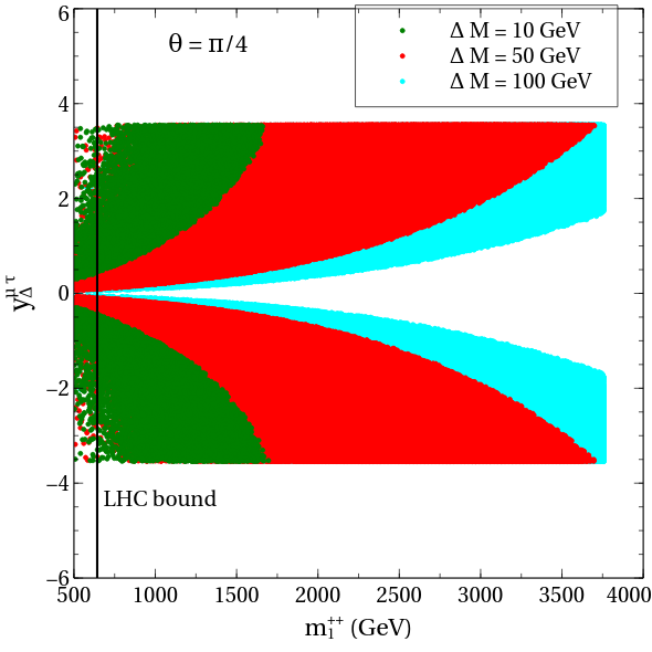
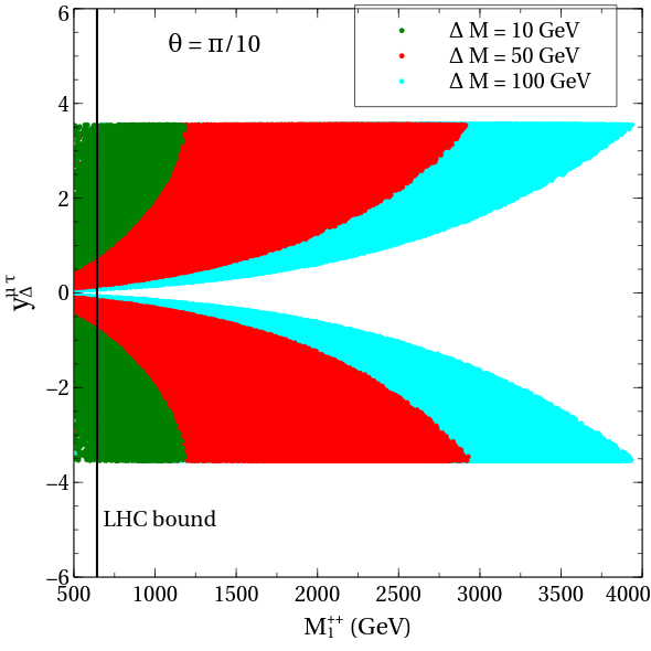
Figure 1: The allowed parameter space maintaining $\Delta a_{\mu}$ within its 2$\sigma$ range in the $M_{1}^{++}-y_{\Delta}^{\mu\tau}$ plane for $\theta=\frac{\pi}{4}$ (left) and $\frac{\pi}{10}$ (right). The color coding is explained in the legends. The $M_{1}^{++}$ values left to the vertical line are disallowed by like-sign dilepton searches at the LHC CMS:2017pet .

Fig. 1 shows the allowed parameter space in the $M_{1}^{++}$–$y_{\Delta}^{\mu\tau}$ plane for the choices of $\Delta M=10,~{}50,~{}100$ GeV in green, red and cyan, respectively and for $\theta=\frac{\pi}{4}$ (left plot) and $\frac{\pi}{10}$ (right plot). The contribution to $\Delta a_{\mu}$ from $H^{+}$ is roughly given by $\frac{-(y_{\Delta}^{\mu\tau})^{2}}{48\pi^{2}}\frac{m^{2}_{\mu}}{M_{H^{+}}^{2}}$, whereas the chirality flipping term from $H^{++}$ in this model has

$$\Delta a_{\mu}\simeq\frac{y_{\Delta}^{\mu\tau}y_{S}^{\mu\tau}}{16\pi^{2}}\frac{m_{\mu}m_{\tau}}{(M_{1}^{++})^{3}}\Delta Ms_{\theta}c_{\theta}\log\frac{m^{2}_{\tau}}{(M_{1}^{++})^{2}}~{}.$$ (26)

In comparison, the singly charged contribution is suppressed by roughly a factor of $m_{\tau}\Delta M/m^{2}_{\mu}$ for $M_{H^{+}}\simeq M_{1}^{++}$ and $y_{S}^{\mu\tau}\simeq y_{\Delta}^{\mu\tau}$, thereby rendering the doubly charged scalars the dominant contributors. Two crucial parameters in this case are therefore $\theta$ and $\Delta M$. A higher $\Delta M$ implies a larger positive contribution to $\Delta a_{\mu}$. For a fixed value of $\Delta a_{\mu}$, a higher value of $\Delta M$ also implies a higher maximally allowed value for $M_{1}^{++}$. For example, the left plot in Fig. 1 shows $M_{1}^{++}\lesssim 3.7$ TeV in case of $\Delta M=50$ GeV and $M_{1}^{++}\lesssim 1.7$ TeV in case of $\Delta M=10$ GeV. The scalar coupling $\lambda_{7}$ hits its perturbative limit for $\Delta M=100$ GeV and $\theta=\frac{\pi}{4}$, thereby disfavoring $M_{1}^{++}\gtrsim 3.75$ TeV for this particular choice. This explains the sharp vertical boundary in the left plot. In addition, $\theta=\frac{\pi}{4}$ maximizes $\Delta a_{\mu}$ when the other parameters are held fixed. This leads to the expectation that the allowed range of $M_{1}^{++}$ will be the most relaxed. This is again confirmed in the plots, where for $\Delta M=50$ GeV, $M_{1}^{++}\lesssim 3.6$ TeV for $\theta=\frac{\pi}{4}$ while $M_{1}^{++}\lesssim 2.9$ TeV for $\theta=\frac{\pi}{10}$.

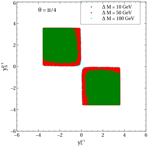
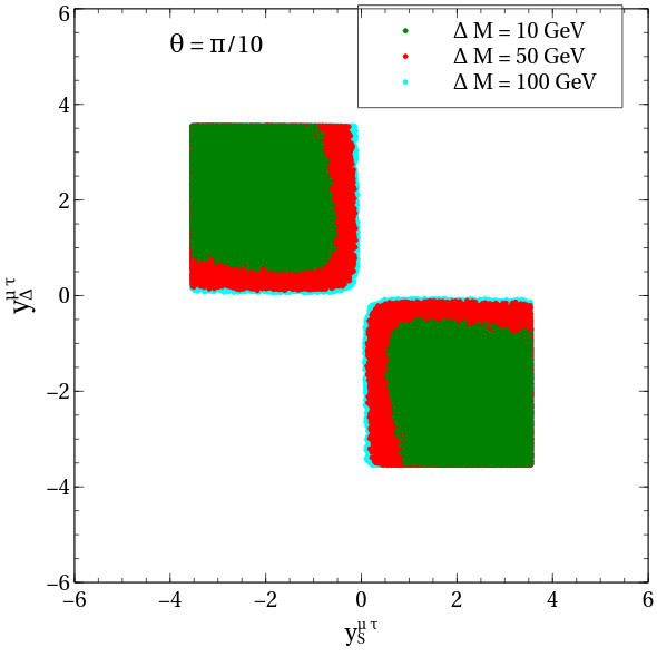
Figure 2: The allowed parameter space maintaining $\Delta a_{\mu}$ within its 2$\sigma$ range in the $y_{\Delta}^{\mu\tau}-y_{S}^{\mu\tau}$ plane for $\theta=\frac{\pi}{4}$ (left) and $\frac{\pi}{10}$ (right). The color coding is explained in the legends.

The same parameter points are plotted in the $y_{\Delta}^{\mu\tau}$–$y_{S}^{\mu\tau}$ plane in Fig. 2. It is seen that points are distributed along the entire ranges of both Yukawa couplings whenever $\Delta M=100$ GeV. The same allowed ranges for both couplings can be traced back to the invariance of the chirality flip under $y_{\Delta}^{\mu\tau}\leftrightarrow y_{S}^{\mu\tau}$. For lower $\Delta M$ values, low values of the Yukawa couplings tend to be disfavored, albeit the reduction in the parameter space is not appreciable. Hence, no strong constraint is imposed by $\Delta a_{\mu}$ in this parameter space.

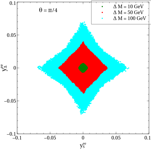
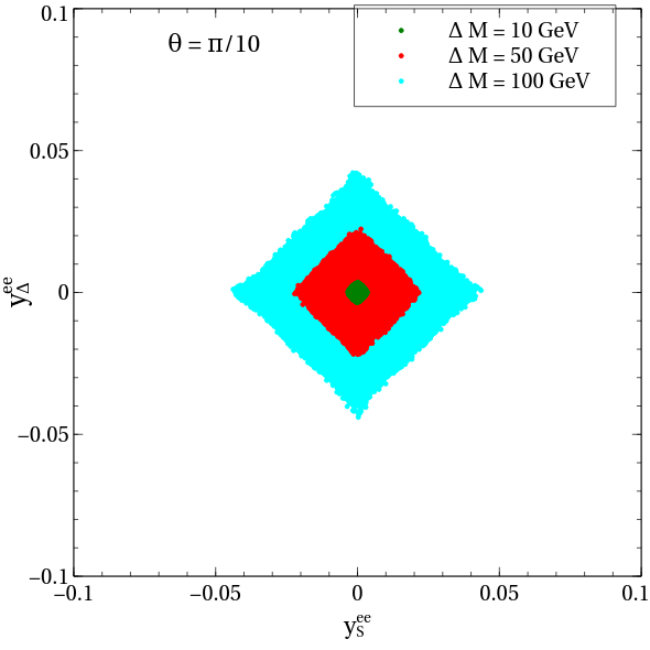
Figure 3: The allowed parameter space maintaining $\Delta a_{\mu}$ within its 2$\sigma$ range in the $y_{\Delta}^{ee}-y_{S}^{ee}$ plane for $\theta=\frac{\pi}{4}$ (left) and $\frac{\pi}{10}$ (right). The color coding is explained in the legends.

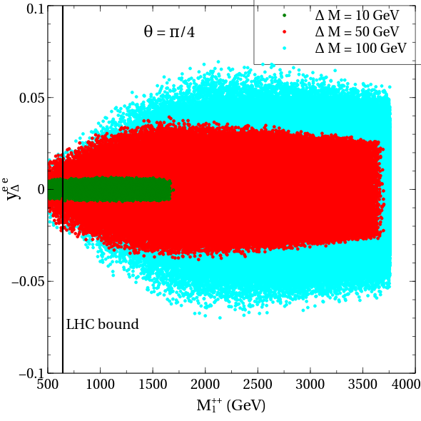
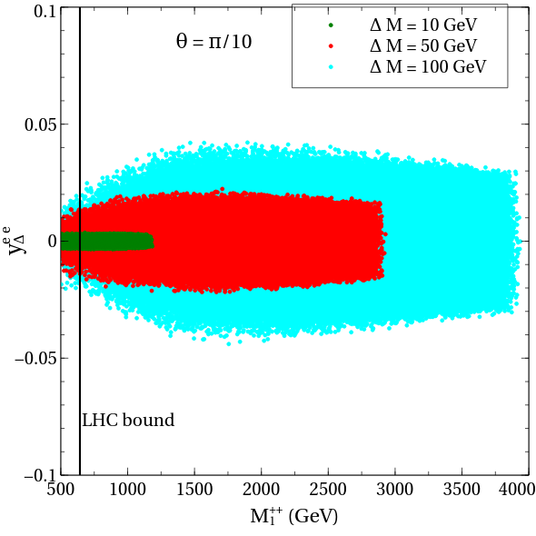
Figure 4: The allowed parameter space maintaining $\Delta a_{\mu}$ within its 2$\sigma$ range in the $y_{\Delta}^{ee}-y_{S}^{ee}$ plane for $\theta=\frac{\pi}{4}$ (left) and $\frac{\pi}{10}$ (right). The color coding is explained in the legends. The $M_{1}^{++}$ values left of the vertical line are disallowed by like-sign dilepton searches at the LHC.

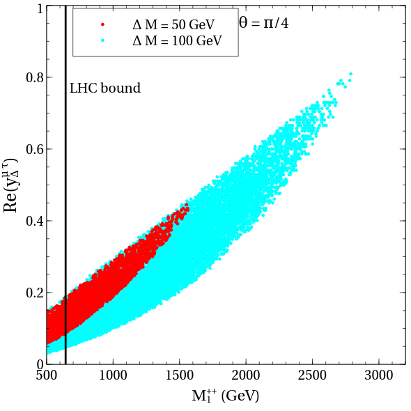
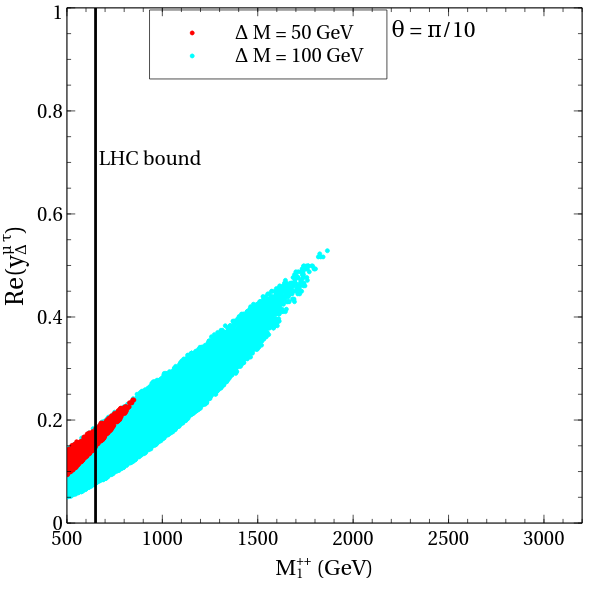
Figure 5: The allowed parameter space maintaining $\Delta a_{\mu}$ within its 2$\sigma$ range and ${\rm BR}_{\tau\rightarrow\bar{\mu}ee}$ within the quoted limit in the $M_{1}^{++}-{\rm Re}(y_{\Delta}^{\mu\tau})$ plane for $\theta=\frac{\pi}{4}$ (left) and $\frac{\pi}{10}$ (right). A normal neutrino mass hierarchy is assumed. The color coding is explained in the legends. The region left to the black line is disallowed by the dilepton searches at the LHC.

We have taken ${\rm BR}_{\tau\rightarrow\mu\nu\nu}\simeq 1/6$ while determining ${\rm BR}_{\tau\rightarrow\bar{\mu}ee}$ using Eq. (24). The prediction of the $\tau\rightarrow\bar{\mu}ee$ rate is correlated with that of $\Delta a_{\mu}$, much due to their dependence on a common set of model parameters, as is evident from Eq. (21c) and Eq. (24). Firstly, the allowed range of $|y_{S}^{ee}|$ is similar to that of $|y_{\Delta}^{ee}|$ (see Fig. 3). As illustrated in this section, the mass splitting $\Delta M$ becomes crucial in determining the maximum of $M_{1}^{++}$, from the consideration of $\Delta a_{\mu}$. And the allowed ranges of $y_{\Delta}^{\mu\tau}$ and $y_{S}^{\mu\tau}$ obviously depend on the overall mass scale of doubly charged scalars. That is, a larger allowed band for $M_{1}^{++}$ loosens the allowed ranges for $y_{\Delta}^{\mu\tau}$ and $y_{S}^{\mu\tau}$. This is corroborated by an inspection of Figs. 3 and 4. In the case of $\theta=\frac{\pi}{4}$, $|y_{\Delta}^{ee}|<10^{-2}$ is obtained for $\Delta M=10$ GeV while the corresponding bound settles at $\simeq 0.07$ for $\Delta M=100$ GeV. The bound for $\Delta M=50$ GeV, as expected, is somewhere in between. The qualitative behavior of the parameter space for other values of $\theta$ and $\Delta M$ can be readily understood from this discussion.

We add here that the results of the numerical scans presented in this section are not affected by the details in the neutrino sector. This is so because a neutrino mass matrix complying with the latest data can always be reconstructed in this model by tuning the trilinear parameters accordingly, as we shall see in the next subsection. The same parameters do not enter the calculations of $\Delta a_{\mu}$ and the LFV rates.

3.2 Neutrino mass matrix

We discuss details of neutrino mass generation in this section. Similar to what happens in the Zee-Babu model, non-zero mass for the neutrinos arises at the two-loop level in this framework. Representative Feynman graphs are shown in Fig. 6.

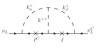
(a)

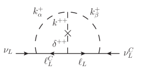
(b)

Figure 6: Two-loop graphs responsible for neutrino mass generation.

We point out here that the amplitude in Fig. 6a is similar to the usual Zee-Babu amplitude as far as its chirality structure is concerned. In contrast, the amplitude in Fig. 6b is induced by the $\delta^{++}$–$k^{++}$ mixing in one of the scalar lines. A different chirality structure renders it much more enhanced compared to Fig. 6a. Explicitly, the neutrino mass matrix elements in this model are given by:

$$m_{\nu}^{\alpha\beta} = \sqrt{2}y_{\Delta}^{\alpha\beta}v_{\Delta}$$ (27)

$$-16\,\sum_{\alpha^{\prime}\beta^{\prime}\alpha^{\prime\prime}\beta^{\prime\prime}}\,\mu_{\alpha^{\prime\prime}\beta^{\prime\prime}}y_{A}^{\alpha^{\prime\prime}}\epsilon^{\alpha\alpha^{\prime}\alpha^{\prime\prime}}y_{A}^{\beta^{\prime\prime}}\epsilon^{\beta\beta^{\prime}\beta^{\prime\prime}}\Big{\{}y^{\alpha^{\prime}\beta^{\prime}}_{S}\,\Big{[}s^{2}_{\theta}I_{k1}^{\alpha^{\prime\prime}\beta^{\prime\prime}\alpha^{\prime}\beta^{\prime}}+c^{2}_{\theta}I_{k2}^{\alpha^{\prime\prime}\beta^{\prime\prime}\alpha^{\prime}\beta^{\prime}}\Big{]}$$

$$\qquad\qquad\qquad+y^{\alpha^{\prime}\beta^{\prime}}_{\Delta}\,s_{\theta}c_{\theta}\,\Big{[}-I_{\Delta 1}^{\alpha^{\prime\prime}\beta^{\prime\prime}\alpha^{\prime}\beta^{\prime}}+I_{\Delta 2}^{\alpha^{\prime\prime}\beta^{\prime\prime}\alpha^{\prime}\beta^{\prime}}\Big{]}\Big{\}},$$

where $I_{Xi}^{\alpha^{\prime\prime}\beta^{\prime\prime}\alpha^{\prime}\beta^{\prime}}\equiv I_{X}(M^{+}_{\alpha^{\prime\prime}},M^{+}_{\beta^{\prime\prime}},M^{++}_{i},m_{\alpha^{\prime}},m_{\beta^{\prime}})$. The $2$-loop integrals $I_{k}(M^{+}_{\alpha},M^{+}_{\beta},M^{++}_{i},m_{\mu},m_{\tau})$ and $I_{\Delta}(M^{+}_{\alpha},M^{+}_{\beta},M^{++}_{i},m_{\mu},m_{\tau})$ have been defined and evaluated in the Appendix.

The $U_{\text{PMNS}}$ matrix diagonalizes the neutrino mass matrix $m_{\nu}$, i.e.,

$$m_{\nu}=U_{\text{PMNS}}^{*}~{}m_{\nu}^{\text{diag}}~{}U_{\text{PMNS}}^{T}~{},$$ (28a)

$$\text{with}~{}U_{\text{PMNS}}=V_{\text{PMNS}}\times\text{diag}(1,e^{i\alpha_{21}/2},,e^{i\alpha_{31}/2})~{}\mbox{and}$$ (28b)

$$V_{\text{PMNS}}=\begin{pmatrix}c_{12}c_{13}&s_{12}c_{13}&s_{13}e^{-i\delta_{CP}}\\ -s_{12}c_{23}-c_{12}s_{23}s_{13}e^{i\delta_{CP}}&c_{12}c_{23}-s_{12}s_{23}s_{13}e^{i\delta_{CP}}&s_{23}c_{13}\\ s_{12}s_{23}-c_{12}c_{23}s_{13}e^{i\delta_{CP}}&-c_{12}s_{23}-s_{12}c_{23}s_{13}e^{i\delta_{CP}}&c_{23}c_{13}\end{pmatrix}~{},$$ (28c)

where $s_{ij}=\sin\theta_{ij}$, $c_{ij}=\cos\theta_{ij}$, $\delta_{CP}$ is the Dirac phase, and $\alpha_{21}$ and $\alpha_{31}$ are the Majorana phases.

Before proceeding further, a comment on the relative magnitudes of $I_{k}$ and $I_{\Delta}$ is in order. Due to different chirality structures, $I_{k}/I_{\Delta}\sim\mathcal{O}(m^{2}_{\ell}/M^{2}_{S})$, where $m_{\ell}$ and $M_{S}$ denote a lepton mass and a scalar mass, respectively. Any contribution from $I_{k}$ can hence be neglected for this model. One may refer to Ref. McDonald:2003zj and some references therein to gain additional insight in the two-loop functions.

We have fitted the neutrino oscillation data using our model in the following approach. An $m_{\nu}^{\alpha\beta}$ has six complex entries that are derivable from the neutrino oscillation parameters (see Eq. (28a)). There are 6 complex $\mu_{\alpha\beta}$ in this model. Each $\mu_{\alpha\beta}$ can therefore be solved for from Eq. (27). We recall that all the Yukawa couplings are taken to be real and therefore $\mu_{\alpha\beta}$ are necessarily complex in order to account for the phases coming from $\delta_{CP},\alpha_{21}$ and $\alpha_{31}$.

One can make the following order-of-magnitude estimate for $\mu_{\alpha\beta}$. First, let’s assume $v_{\Delta}=10^{-15}$ GeV so that there is no noticeable contribution from $\langle\Delta\rangle$ to any of the neutrino mass elements. Then for $M_{\alpha}^{+}\simeq 800$ GeV, $M_{i}^{++}\simeq 1$ TeV, the $I_{\Delta}$ integral is of $\mathcal{O}(10^{-4})$. Considering a typical $m_{\nu}^{\alpha\beta}$ having an absolute value around $\mathcal{O}(10^{-3})$ eV and assuming the Yukawa couplings of $\mathcal{O}(1)$, the $\mu_{\alpha\beta}$ value is about $\mathcal{O}(10^{-8})$ GeV. As expected, this is several orders of magnitude smaller than what it would have been in case where only the Zee-Babu-like amplitude (Fig. 6a) is present. Noting that the new $2$-loop amplitude as shown in Fig. 6b survives only in the $\theta\neq 0$ limit, we deem this observation a fallout of the $\Delta$–$k^{++}$ mixing. Therefore, this mixing plays a pivotal role in neutrino mass generation, much like it plays in explaining the muon $g-2$ anomaly.

The full allowed ranges of $\mu_{\alpha\beta}$ can be revealed through a parameter scan. The singly charged scalars are assigned with masses $\simeq$ 800 GeV. Besides, $M_{1}^{++}$ and the Yukawa couplings are varied in the same ranges as in the previous section. In addition, the neutrino oscillation parameters are fixed to their central values Patrignani:2016xqp as

$$\text{sin}^{2}\theta_{12}=0.307~{},~{}~{}\text{sin}^{2}\theta_{23}=0.510~{},~{}~{}\text{sin}^{2}\theta_{13}=0.021~{},$$

$$\Delta m^{2}_{21}=7.45\times 10^{-5}~{}\text{GeV}^{2}~{},~{}\Delta m^{2}_{32}=2.53\times 10^{-3}~{}\text{GeV}^{2}~{},$$

$$\delta_{CP}=1.41\pi~{},~{}~{}\alpha_{21}=\alpha_{31}=0~{}.$$ (29)

The mass of the lightest neutrino and Majorana phases are assumed to vanish in the present analysis. In addition to imposing the constraints of $\Delta a_{\mu}$, LFV bounds and $|\lambda_{7}|<4\pi$, we also perform the a perturbativity check of the trilinear parameters, i.e., $|\mu_{\alpha\beta}|<4\pi~{}\text{min}(M^{++}_{i},M^{+}_{\alpha})$. Figs. 7 and 8 depict the real and imaginary parts of $\mu_{\alpha\beta}$ that are required to explain the neutrino data for normal as well as inverted mass orderings, respectively. In order to understand the linear shape of these plots, consider that $\mu_{\mu\tau}\propto m_{\nu}^{ee}$, with the proportionality factor being real (since the Yukawa couplings are real). One then can write

$$\frac{\text{Re}(\mu_{\mu\tau})}{\text{Im}(\mu_{\mu\tau})} = \frac{\text{Re}(m_{\nu}^{ee})}{\text{Im}(m_{\nu}^{ee})}$$ (30)

Now, the right hand side of Eq. (30) is fixed and this in turn fixes the slope of the parameter points in the $|\text{Re}(\mu_{\mu\tau})|$–$|\text{Im}(\mu_{\mu\tau})|$ plane. This pattern is also seen in case of trilinear parameters other than $\mu_{ee}$. And this difference comes from the fact that the expression for $m_{\nu}^{\mu\tau}$ constrains contributions from both $\mu_{ee}$ and $\mu_{\mu\tau}$. The linear shape obviously will get smeared once a variation of the neutrino oscillation parameters is invoked.

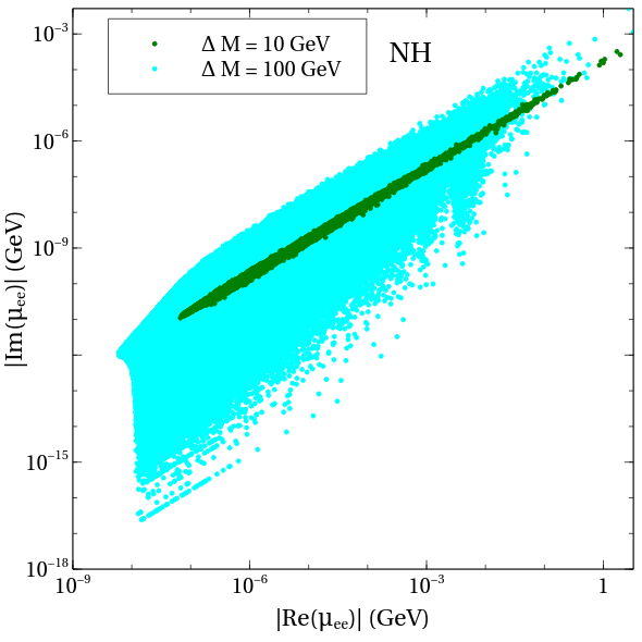
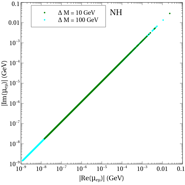
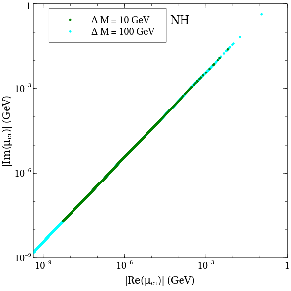
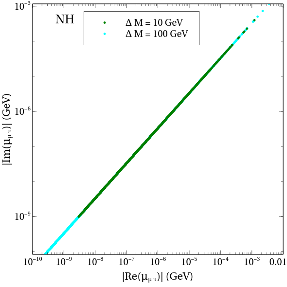
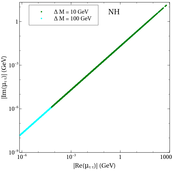
Figure 7: Allowed values of $\mu_{\alpha\beta}$ in the case of normal hierarchy (NH), plotted in the plane of real vs imaginary axes. The color coding can be read from the legends.

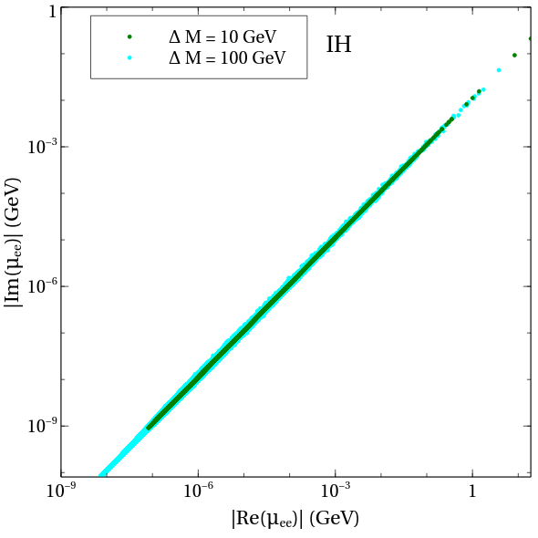
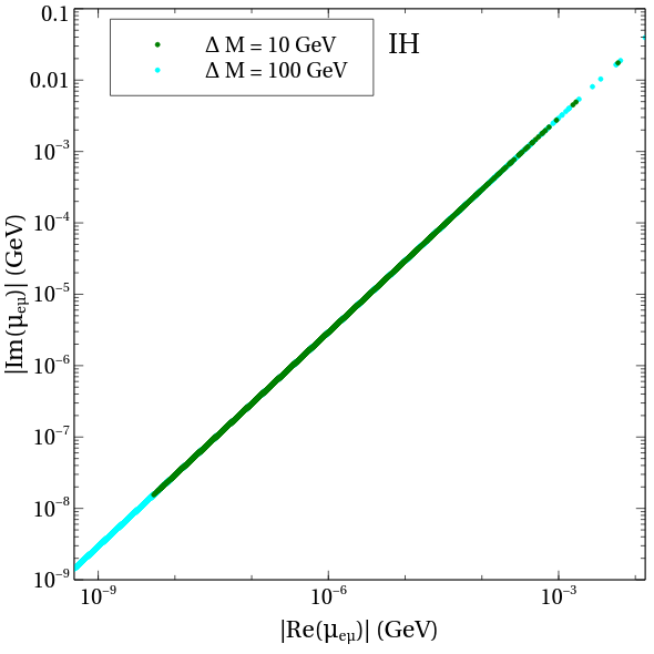
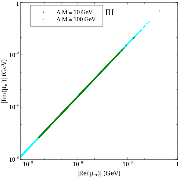
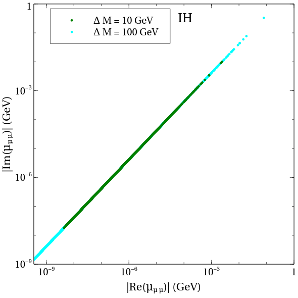
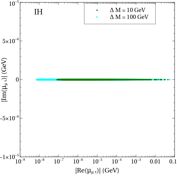
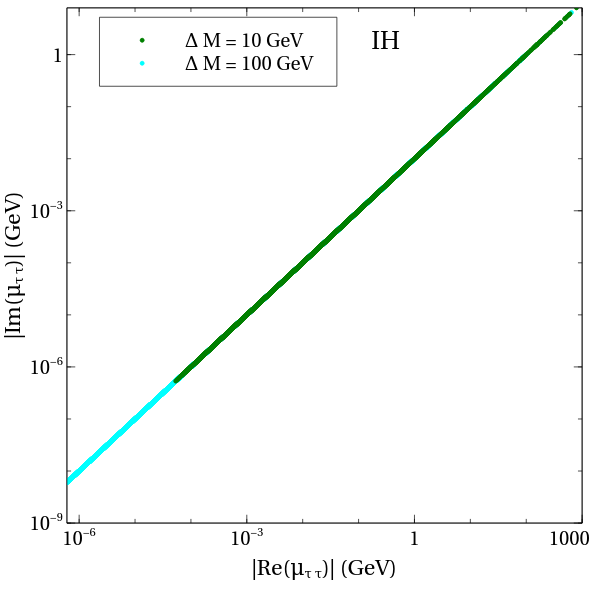
Figure 8: Allowed values of $\mu_{\alpha\beta}$ in the case of inverted hierarchy (IH), plotted in the plane of real vs imaginary axes. The color coding can be read from the legends.

We comment here that the above analyses can be repeated for a larger value of $v_{\Delta}$. In such a case, the contribution of the triplet to the $(ee)$ and $(\mu\tau)$ elements can be appreciable and, in fact, much larger than the mass scale of the light neutrinos in principle. If so, $|\mu_{\mu\tau}|$ and $|\mu_{ee}|$ also have to be suitably large so as to make way for a cancellation between the tree-level and two-loop terms. Therefore, no strong constraint on the triplet VEV emerges in this scenario from the consideration of neutrino mass.

4 Numerical results: Scenario B

In this section, we demonstrate the viability of Scenario B in connection to the muon $g-2$ anomaly, neutrino mass and LFV processes. As we will see below, the predictions of $\Delta a_{\mu}$ and LFV are expected to be sharply correlated with the neutrino masses and mixings for the present scenario. Therefore, we do not divide our discussions into different subsections, as was the approach taken in the case of Scenario A, owing to a different neutrino mass mechanism in that case. The contributions to muon $g-2$ coming from the singly and doubly charged scalars add up as follows:

$$\Delta a_{\mu}=\Delta a^{\Delta^{+}}_{\mu}+\Delta a^{\Delta^{++}}_{\mu}+\sum_{i=1,2}\Delta a^{H_{i}^{++}}_{\mu},$$ (31)

where

$$\Delta a^{\Delta^{+}}_{\mu} = -\frac{m_{\mu}^{2}}{8\pi^{2}}{|y_{\Delta}^{\mu\tau}|}^{2}\int_{0}^{1}dx\frac{x(1-x)}{(M_{e}^{+})^{2}-m^{2}_{\mu}(1-x)}$$ (32a)

$$-\frac{m_{\mu}^{2}}{8\pi^{2}}{|y_{\Delta}^{\mu\mu}|}^{2}\int_{0}^{1}dx\frac{x(1-x)}{(M_{\mu}^{+})^{2}-m^{2}_{\mu}(1-x)}$$

$$-\frac{m_{\mu}^{2}}{8\pi^{2}}{|y_{\Delta}^{e\mu}|}^{2}\int_{0}^{1}dx\frac{x(1-x)}{(M_{\tau}^{+})^{2}-m^{2}_{\mu}(1-x)},$$

$$\Delta a^{H_{i}^{++}}_{\mu} = -\frac{m_{\mu}^{2}}{4\pi^{2}}\int_{0}^{1}dx\frac{(|y^{\mu\tau}_{iL}|^{2}+|y^{\mu\tau}_{iR}|^{2})(1-x)+2~{}\text{Re}[y^{\mu\tau}_{iL}y^{\mu\tau}_{iR}](m_{\tau}/m_{\mu})}{m^{2}_{\mu}x^{2}+(m^{2}_{\tau}-m^{2}_{\mu})x+(M^{++}_{i})^{2}(1-x)}x^{2}$$ (32b)

$$-~{}\frac{m^{2}_{\mu}}{2\pi^{2}}\int_{0}^{1}dx~{}\frac{(|y^{\mu\tau}_{iL}|^{2}+|y^{\mu\tau}_{iR}|^{2})x+2~{}\text{Re}[y^{\mu\tau}_{iL}y^{\mu\tau}_{iR}](m_{\tau}/m_{\mu})}{m^{2}_{\mu}x^{2}+((M^{++}_{i})^{2}-m^{2}_{\mu})x+m^{2}_{\tau}(1-x)}x(1-x),$$

$$\Delta a^{\Delta^{++}}_{\mu} = -\frac{m_{\mu}^{2}|y_{\Delta}^{\mu\mu}|^{2}}{4\pi^{2}}\int_{0}^{1}dx\frac{x^{2}(1-x)}{m^{2}_{\mu}x^{2}+(m^{2}_{\tau}-m^{2}_{\mu})x+(M^{++}_{\mu})^{2}(1-x)}$$ (32d)

$$-~{}\frac{m^{2}_{\mu}|y_{\Delta}^{\mu\mu}|^{2}}{2\pi^{2}}\int_{0}^{1}dx~{}\frac{x^{2}(1-x)}{m^{2}_{\mu}x^{2}+((M^{++}_{\mu})^{2}-m^{2}_{\mu})x+m^{2}_{\tau}(1-x)}$$

$$-\frac{m_{\mu}^{2}|y_{\Delta}^{e\mu}|^{2}}{4\pi^{2}}\int_{0}^{1}dx\frac{x^{2}(1-x)}{m^{2}_{\mu}x^{2}+(m^{2}_{\tau}-m^{2}_{\mu})x+(M^{++}_{\tau})^{2}(1-x)}$$

$$-~{}\frac{m^{2}_{\mu}|y_{\Delta}^{e\mu}|^{2}}{2\pi^{2}}\int_{0}^{1}dx~{}\frac{x^{2}(1-x)}{m^{2}_{\mu}x^{2}+((M^{++}_{\tau})^{2}-m^{2}_{\mu})x+m^{2}_{\tau}(1-x)}.$$

The absence of a chirality-flipping term in the contributions from $H_{\mu,\tau}^{++}$ is expected and, therefore, one observes $\Delta a^{\Delta^{++}}_{\mu}<0$.

LFV decays of $\tau\rightarrow\bar{\mu}ee$ and $\tau\rightarrow\bar{e}\mu\mu$ are allowed by the underlying $\mathbb{Z}_{3}$ symmetry. Of these, the branching fraction formula for the former process is the same as Eq. (24) in Scenario A. The branching fraction for the latter is given by

$${\rm BR}_{\tau\rightarrow\bar{e}\mu\mu} = \frac{|y_{\Delta}^{e\tau}|^{2}|y_{\Delta}^{\mu\mu}|^{2}}{4G_{F}^{2}(M_{\tau}^{++})^{4}}~{}.$$ (33a)

The independent parameters here are $M^{+}_{\alpha},M^{++}_{i},v_{\alpha},y_{S}^{\mu\tau}$, $y_{S}^{ee}$ and $\theta$. The muon $g-2$ is most sensitive to $M_{i}^{++},y_{\Delta}^{\mu\tau}$ and $y_{S}^{\mu\tau}$. Among these, $y_{\Delta}^{ee}$ and $y_{\Delta}^{\mu\tau}$ can be fixed by the neutrino mass matrix elements as $y_{\Delta}^{ee}=\frac{m^{ee}_{\nu}}{\sqrt{2}v_{e}}$ and $y_{\Delta}^{\mu\tau}=\frac{m^{\mu\tau}_{\nu}}{\sqrt{2}v_{e}}$. The following model parameter variation is made:

$$500~{}\text{GeV}<M_{1}^{++}<5~{}\text{TeV}~{},$$ (34a)

$$|y_{S}^{\mu\tau}|,|y_{S}^{ee}|<\sqrt{4\pi}~{},$$ (34b)

$$10^{-14}~{}\text{GeV}<v_{e}<10^{-4}~{}\text{GeV}~{}.$$ (34c)

In an approach similar to Scenario A, the representative values $\Delta M$ = 50 GeV, 100 GeV, $M_{1}^{+}=M_{1}^{++}$ and $\theta=\frac{\pi}{4},\frac{\pi}{10}$ are assigned. The remaining model parameters contribute only at subleading order to $\Delta a_{\mu}$, leading us to fix $M_{\mu}^{+}=1$ TeV, $M_{\tau}^{+}=1.2$ TeV, and $M_{\mu}^{++}=M_{\tau}^{++}=1.1$ TeV. The neutrino oscillation parameters are fixed to their central values as shown in Eq. (29).

With Eq. (33a), ${\rm BR}_{\tau\rightarrow\bar{e}\mu\mu}<10^{-8}$ is translated to

$$v_{\mu}\gtrsim\frac{v}{M_{\tau}^{++}}\sqrt{\frac{|m_{\nu}^{e\tau}|}{\text{1 eV}}\frac{|m_{\nu}^{\mu\mu}|}{\text{1 eV}}}\times 10^{-7}~{}\text{GeV}~{}.$$ (35)

For typical values of $M_{\tau}^{++}\simeq 1$ TeV and $|m_{\nu}^{e\tau}|,~{}|m_{\nu}^{e\tau}|\simeq 0.1$ eV, we get $v_{\mu}\gtrsim 2.5\times 10^{-9}$ GeV. We have therefore chosen $v_{\mu}=v_{\tau}=10^{-8}$ GeV in this analysis to ensure a suppressed rate for $\tau\rightarrow\bar{e}\mu\mu$. Also, once all the triplet VEV’s are fixed, all $y_{\Delta}^{\alpha\beta}$ can be determined from the neutrino mass matrix. Note that this choice for $v_{e}$ and $v_{\tau}$ renders the contributions of $H_{\mu}^{++}$ and $H_{\tau}^{++}$ to $\Delta a_{\mu}$ negligible. In the following, we plot the parameter points favoring a $\Delta a_{\mu}$ in the 2$\sigma$ interval, a perturbative $\lambda_{7}$ and sufficiently small decay rate in the $\tau\rightarrow\bar{\mu}ee$ channel in various planes of the parameter space.

It is important to highlight how the present scenario numerically differs from Scenario A. First, the allowed parameter space in the current scenario shows similar trends as in the case of Scenario A (see Fig. 1), much due to a common mechanism to explain $\Delta a_{\mu}$. However, a main difference lies in the fact that $y_{\Delta}^{\mu\tau}$ is now proportional to $m_{\nu}^{\mu\tau}$. This correlation gives the restriction $|\text{Re}(y_{\Delta}^{\mu\tau})|<0.8$ for $\Delta M=100$ GeV. On the other hand, the corresponding bound is more relaxed in case of Scenario A, as seen by a comparison between Fig. 5 and Fig. 1. In a way, Fig. 5 can be seen as a constrained version of Fig. 1. Given that the chirality flip contribution is proportional to $\sim\Delta Ms_{\theta}c_{\theta}y_{\Delta}^{\mu\tau}y_{S}^{\mu\tau}$, a lower $|y_{\Delta}^{\mu\tau}|$ in Scenario B calls for a higher $\Delta M$ and/or a lower $M_{1}^{++}$ in order to maintain the muon enhancement at the same magnitude.

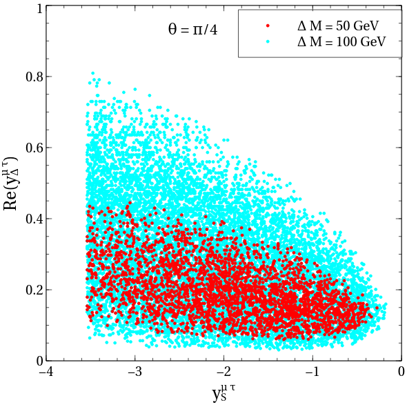
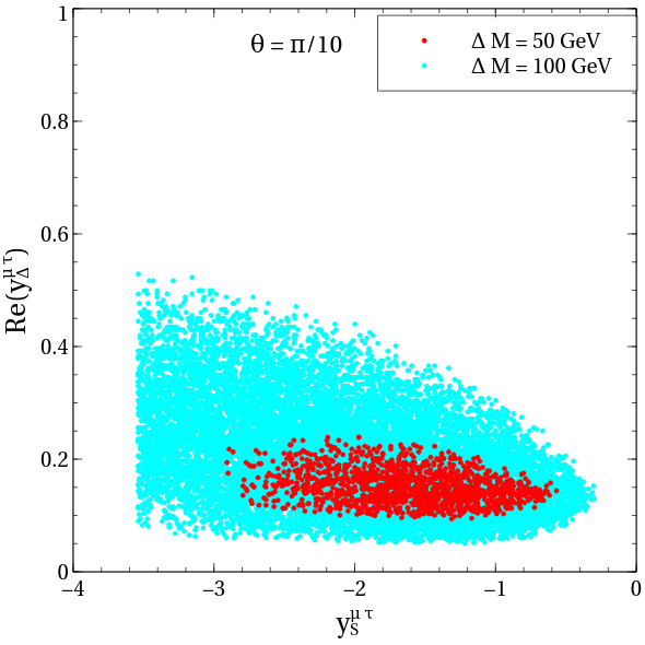
Figure 9: The allowed parameter space maintaining $\Delta a_{\mu}$ within its 2$\sigma$ range and ${\rm BR}_{\tau\rightarrow\bar{\mu}ee}$ within the quoted limit in the $y_{S}^{\mu\tau}-\text{Re}(y_{\Delta}^{\mu\tau})$ plane for $\theta=\frac{\pi}{4}$ (left) and $\frac{\pi}{10}$ (right). A normal neutrino mass hierarchy is assumed. The color coding is explained in the legends.

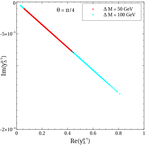
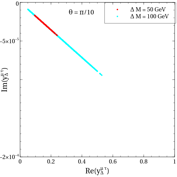
Figure 10: Scatter points maintaining $\Delta a_{\mu}$ within its 2$\sigma$ range and $\text{BR}_{\tau\rightarrow\bar{\mu}ee}$ within the quoted limit plotted in the $\text{Re}(y_{\Delta}^{\mu\tau})-\text{Im}(y_{\Delta}^{\mu\tau})$ plane for $\theta=\frac{\pi}{4}$ (left) and $\frac{\pi}{10}$ (right). A normal neutrino mass hierarchy is assumed. The color coding is explained in the legends.

In Fig. 9 together with Fig. 10, we show the allowed parameter space in the $y_{\Delta}^{\mu\tau}$–$y_{S}^{\mu\tau}$ plane. These plots characterize the contributions to muon $g-2$, and should be compared with Fig. 2 in Scenario A. Because of the proportionality relation $m_{\nu}^{\mu\tau}\propto y_{\Delta}^{\mu\tau}$, the parameter $y_{\Delta}^{\mu\tau}$ is constrained more severely in Scenario B for a given $v_{e}$. In order to fit the neutrino oscillation data, the real part and the imaginary part of $y_{\Delta}^{\mu\tau}$ are strongly correlated, as shown in Fig. 10. This correlation is somewhat similar to the relation between $\mu_{\alpha\beta}$ and $m_{\nu}^{\alpha\beta}$ in Scenario A (see also Figs. 7 and 8).

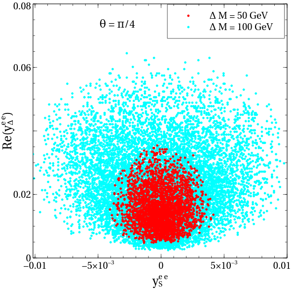
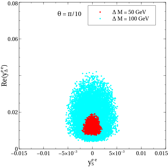
Figure 11: Scatter points maintaining $\Delta a_{\mu}$ within its 2$\sigma$ range and ${\rm BR}_{\tau\rightarrow\bar{\mu}ee}$ within the quoted limit plotted in the $y_{S}^{ee}-\text{Re}(y_{\Delta}^{ee})$ plane for $\theta=\frac{\pi}{4}$ (left) and $\frac{\pi}{10}$ (right). A normal neutrino mass hierarchy is assumed. The color coding is explained in the legends.

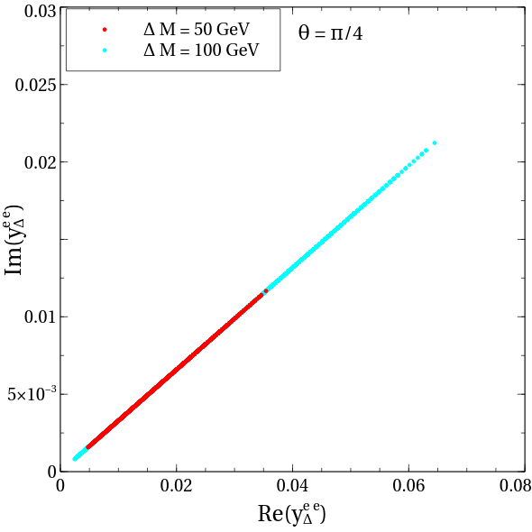
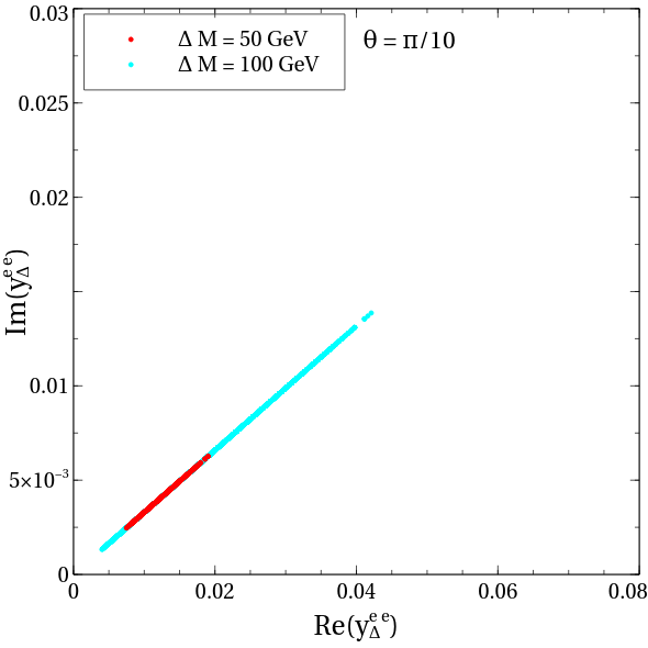
Figure 12: Points maintaining $\Delta a_{\mu}$ within its 2$\sigma$ range and $\text{BR}_{\tau\rightarrow\bar{\mu}ee}$ within the quoted limit plotted in the $\text{Re}(y_{\Delta}^{ee})-\text{Im}(y_{\Delta}^{ee})$ plane for $\theta=\frac{\pi}{4}$ (left) and $\frac{\pi}{10}$ (right). A normal neutrino mass hierarchy is assumed. The color coding is explained in the legends.

The couplings $y_{\Delta}^{\mu\tau}$ and $y_{\Delta}^{ee}$ that enter the expression for the $\tau\rightarrow\bar{\mu}ee$ branching fraction are dictated by the size of the $(ee)$ and $(\mu\tau)$ neutrino mass matrix elements, respectively. Therefore, the choice of the neutrino mass hierarchy becomes crucial in the analysis. In the case of NH, $|m_{\nu}^{ee}|\sim\mathcal{O}(10^{-3})$ eV throughout the entire space allowed by the oscillation data. However, the same is $\mathcal{O}(10^{-2})$ eV for the IH case, causing the $\tau\rightarrow\bar{\mu}ee$ branching ratio to overshoot the allowed limit by a factor of $\sim\mathcal{O}(10^{2})$. Consequently, no parameter point survives in the case of IH when the muon $g-2$ and LFV constraints are considered simultaneously.

We read from Fig. 11 that the bound on $|y_{\Delta}^{ee}|$ is about 0.07 for $\theta=\frac{\pi}{4}$ and settles to about 0.05 for $\theta=\frac{\pi}{10}$. These numbers are close to the corresponding numbers in Scenario A. However, $y_{S}^{ee}$ is more constrained in the present case. This is attributed to the fact that $|y_{\Delta}^{\mu\tau}|$ is more tightly constrained in Scenario B. ${\rm BR}_{\tau\rightarrow\bar{\mu}ee}$ therefore allows the bound on $y_{\Delta}^{ee}$ to be loosened accordingly. For completeness, we also display the imaginary part of $y_{\Delta}^{ee}$ in Fig. 12.

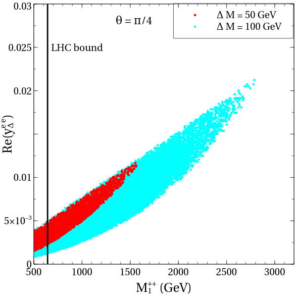
Figure 13: Scatter points maintaining $\Delta a_{\mu}$ within its 2$\sigma$ range and ${\rm BR}_{\tau\rightarrow\bar{\mu}ee}$ within the quoted limit plotted in the $M_{1}^{++}-\text{Re}(y_{\Delta}^{ee})$ plane for $\theta=\frac{\pi}{4}$ (left) and $\frac{\pi}{10}$ (right). A normal neutrino mass hierarchy is assumed. The color coding is explained in the legends. The region left to the black line is disallowed by dilepton searches at the LHC.

In Fig. 13, we show the allowed parameter space in the $y_{\Delta}^{ee}$–$M_{1}^{++}$ plane. Here, we take $\theta=\frac{\pi}{4}$ and $\Delta M=50$ GeV, and find that $\Delta a_{\mu}$ in its 2$\sigma$ range disfavors $M_{1}^{++}\gtrsim 1.6$ TeV. The corresponding disfavored range stands at $M_{1}^{++}\gtrsim 3.7$ TeV in Scenario A. In the same logic, $\Delta M=10$ GeV is disfavored in Scenario B as it does not provide the required $\Delta a_{\mu}$ enhancement. A reduction in the parameter space after switching from the maximal mixing ($\theta=\frac{\pi}{4}$) to another angle ($\theta=\frac{\pi}{10}$ here) is expected and seen in all the plots.

The triplet VEV $v_{e}$ turns out to be bounded from both above and below in Scenario B, as seen in Fig. 14. This is because the maximally (minimally) allowed values of $y_{\Delta}^{\mu\tau}$ and $y_{\Delta}^{ee}$ passing the constraints come from the minimum (maximum) of $v_{e}$ for given $m_{\nu}^{\mu\tau}$ and $m_{\nu}^{ee}$. Again, this is in contrast with Scenario A where there is no such bound.

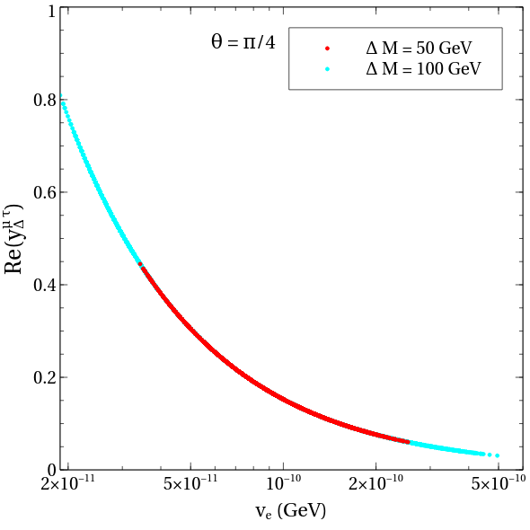
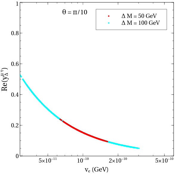
Figure 14: Scatter points maintaining $\Delta a_{\mu}$ within its 2$\sigma$ range and $\text{BR}_{\tau\rightarrow\bar{\mu}ee}$ within the quoted limit in the $v_{e}-\text{Re}(y_{\Delta}^{\mu\tau})$ plane for $\theta=\frac{\pi}{4}$ (left) and $\frac{\pi}{10}$ (right). A normal neutrino mass hierarchy is assumed. The color coding is explained in the legends.

As a closing remark, Scenario B is more constrained than Scenario A, in spite of having a larger number of scalar degrees of freedom. This is because of the Type-II-like $y_{\Delta}\sim\frac{m_{\nu}}{v_{\Delta}}$ relation in the scenario. Therefore, the sizes of the $(ee)$ and $(\mu\tau)$ elements in the neutrino mass matrix are crucial in shaping up the allowed parameter space. Going from Scenario A to Scenario B, the IH becomes disallowed. And this is found to hold true even if the neutrino oscillation parameters are varied within their allowed ranges. However, the parameter regions corresponding to NH open up a bit further in that case. Scenario A enjoys more freedom precisely due to the presence of $\mathbb{Z}_{3}$-breaking trilinear parameters. An appropriate choice of these parameters can reproduce both NH as well as IH without conflict with the muon $g-2$ anomaly and LFV decay bounds.

5 Summary and conclusions

The main theme of the present work is an explanation of the muon $g-2$ anomaly by arranging for a mixing between the doubly charged scalar belonging to an $SU(2)_{L}$ triplet and a doubly charged $SU(2)_{L}$ scalar singlet. The doubly charged mass eigenstates then couple to both chiralities of leptons. In such a case, the chirality flip in the muon $g-2$ loops can induce the requisite positive contribution so as to accommodate the anomaly. We have proposed two models (Scenario A and Scenario B) to investigate this effect. We have also sought to address non-zero neutrino mass and to satisfy the LFV decay constraints at the same time.

In Scenario A, the SM scalar sector is augmented by a complex scalar triplet $\Delta$, a doubly charged scalar singlet $k^{++}$, and three singly charged scalar singlets $k^{+}_{e},k^{+}_{\mu},k^{+}_{\tau}$. A softly broken $\mathbb{Z}_{3}$ symmetry is imposed under which $k^{+}_{e},k^{+}_{\mu},k^{+}_{\tau}$ have charges $1,\omega,\omega^{2}$, respectively, while $\Delta,k^{++}$ have charge 1. However, soft $\mathbb{Z}_{3}$-breaking quadratic and trilinear terms are allowed, thereby causing the singly charged scalars to mix. Neutrino mass arises at the two-loop level and, therefore, this framework is a generalization of the well-known Zee-Babu model. The main findings in this scenario are the following:

• Owing to the $\Delta$–$k^{++}$ mixing, the dipole term corresponding to muon $g-2$ receives a boosted contribution. More precisely, this is due to the chirality flip and a logarithmic term in the loop amplitudes. It therefore becomes possible to address the muon $g-2$ anomaly in this framework.

• The singlet-triplet scalar mixing plays a pivotal role also in the case of neutrino mass. A non-zero mixing induces a new two-loop amplitude that enjoys a chirality enhancement over the usual Zee-Babu-like diagram. In this paper, we have calculated the two-loop integrals exactly, including one which to our knowledge has not been done before. We have shown that by a suitable choice of the soft $\mathbb{Z}_{3}$ breaking trilinear parameters, it is possible to satisfy the present neutrino oscillation data. We have demonstrated it through benchmark points that agree with normal and inverted mass hierarchies.

• In the absence of $\mathbb{Z}_{3}$-breaking quadratic terms, the only non-trivial LFV process is $\tau\rightarrow\bar{\mu}ee$. We have shown that the rate of this process can be maintained within the allowed limit in the parameter region that accounts for the muon $g-2$ anomaly.

• The triplet VEV is allowed to take a wide range of values.

In Scenario B, three scalar triplets $\Delta_{e},\Delta_{\mu},\Delta_{\tau}$ having $\mathbb{Z}_{3}$ charges 1, $\omega,~{}\omega^{2}$ respectively and one doubly charged scalar singlet $k^{++}$, each having $\mathbb{Z}_{3}$ charge 1, are introduced. A violation of $\mathbb{Z}_{3}$ through soft terms is necessary here as neutrino mass is generated at the tree level when the triplets acquire VEV’s. Once again, mixing between between the doubly charged state of $\Delta_{e}$ and $k^{++}$ occurs after EWSB. Some salient features of the allowed parameter region in this case are as follows:

• In this case, the $\Delta_{e}$–$k^{++}$ mixing also paves the way for a chirality flipping contribution in the muon $g-2$ loops. The requisite enhancement in muon $g-2$ is therefore generated in a manner similar to the previous scenario.

• In the case of a normal neutrino mass hierarchy, the parameter space favoring an enhanced muon $g-2$ also complies with the bounds on the branching fractions of $\tau\rightarrow\bar{\mu}ee$ and $\tau\rightarrow\bar{e}\mu\mu$, the only non-vanishing LFV modes in this scenario.

• The present scenario disfavors an inverted neutrino mass hierarchy. This is attributed to the fact that the $m_{\nu}^{ee}$ value associated with the IH is typically larger than the corresponding NH value by at least an order of magnitude. As a result, the rate of $\tau\rightarrow\bar{\mu}ee$ is often predicted above the permitted limit.

• Unlike in Scenario A, the triplet VEV gets bounded from both ends in the process of reconciling the muon $g-2$ anomaly with LFV constraints.

The introduction of any dimension-$2$ $\mathbb{Z}_{3}$-breaking terms in such scenarios will lead to quadratic mixing between the scalars and, therefore, turn on the loop-induced $l_{\alpha}\rightarrow l_{\beta}\gamma$ LFV processes. For both Scenario A and Scenario B, singly charged and doubly charged scalars will be running in the loops. However, the $\mathbb{Z}_{3}$-violating Yukawa interactions so induced will obviously be proportional to the magnitude of the quadratic mixing. Hence, such LFV rates can be easily controlled by keeping the magnitude of the $\mathbb{Z}_{3}$-breaking terms sufficiently small.

Finally, a remark on possible collider signatures of these models is in order. The strengths of the $\mu\tau$ Yukawa couplings of the doubly charged scalars in both scenarios are found to be much larger than the corresponding $ee$ strength. In such a case, $pp\to H^{++}_{1}H^{--}_{2}$ followed by $H^{++}_{1,2}\to$ $\mu^{+}\tau^{+}$ can give rise to a pair of like-sign dilepton $\mu\tau$ with an invariant mass peaking around $M^{++}_{1}$ and $M^{++}_{2}$, respectively. For a sizeable mass gap, these invariant mass peaks would share no overlap. A resolution of these two peaks can enable one to distinguish the proposed scenarios from the pure Type-II model.

Appendix A Appendix

This section contains various analytical expressions related to $\Delta a_{\mu}$ and neutrino mass.

A.1 Muon $g-2$ integrals

The $H_{i}^{++}$ contributions to $\Delta a_{\mu}$ contain the following integrals with $M_{S}$ denoting $M_{1,2}^{++}$:

$$\int_{0}^{1}dx~{}\frac{x^{2}-x^{3}}{m^{2}_{\mu}x^{2}+(m^{2}_{\tau}-m^{2}_{\mu})x+M_{S}^{2}(1-x)}$$

$$=\Big{[}2M_{S}^{6}+3M_{S}^{4}m_{\tau}^{2}-6M_{S}^{2}m_{\tau}^{4}+m_{\tau}^{6}-6M_{S}^{4}m_{\tau}^{2}~{}\text{log}\frac{m^{2}_{\tau}}{M_{S}^{2}}\Big{]}/\Big{[}6(M_{S}^{2}-m_{\tau}^{2})^{2}\Big{]}~{},$$ (36)

$$\int_{0}^{1}dx~{}\frac{x^{2}}{m^{2}_{\mu}x^{2}+(m^{2}_{\tau}-m^{2}_{\mu})x+M_{S}^{2}(1-x)}$$

$$=\Big{[}(M_{S}^{2}-m_{\tau}^{2})\Big{(}-3M_{S}^{4}+4M_{S}^{2}m_{\tau}^{2}-m_{\tau}^{4}+2M_{S}^{4}~{}\text{log}\frac{m^{2}_{\tau}}{M_{S}^{2}}\Big{)}\Big{]}/\Big{[}2(M_{S}^{2}-m_{\tau}^{2})^{2}\Big{]}~{},$$ (37)

$$\int_{0}^{1}dx~{}\frac{x^{2}(x-1)}{m^{2}_{\mu}x^{2}+(M_{S}^{2}-m^{2}_{\mu})x+m^{2}_{\tau}(1-x)}$$

$$=-\Big{[}M_{S}^{6}-6M_{S}^{4}m_{\tau}^{2}+7M_{S}^{2}m_{\tau}^{4}-2m_{\tau}^{6}+6M_{S}^{4}m_{\tau}^{2}~{}\text{log}\frac{m^{2}_{\tau}}{M_{S}^{2}}\Big{]}/\Big{[}6(M_{S}^{2}-m_{\tau}^{2})^{2}\Big{]}~{},$$ (38)

$$\int_{0}^{1}dx~{}\frac{x(x-1)}{m^{2}_{\mu}x^{2}+(M_{S}^{2}-m^{2}_{\mu})x+m^{2}_{\tau}(1-x)}$$

$$=-\Big{[}(M_{S}^{2}-m_{\tau}^{2})\Big{(}M_{S}^{4}m_{\tau}^{4}-2M_{S}^{2}m^{2}_{\tau}~{}\text{log}\frac{m^{2}_{\tau}}{M_{S}^{2}}\Big{)}\Big{]}/\Big{[}2(M_{S}^{2}-m_{\tau}^{2})^{2}\Big{]}~{}.$$ (39)

A.2 Evaluation of $I_{k}(m_{1},m_{2},m,m_{c},m_{d})$

We use the notation in Ref. McDonald:2003zj when calculating the two-loop integrals connected to neutrino mass generation:

$$(m_{1}|m_{2}|m) = \int d^{d}p_{E}d^{d}q_{E}~{}\frac{1}{(p_{E}^{2}+m^{2}_{1})(q_{E}^{2}+m^{2}_{2})((p_{E}+q_{E})^{2}+m^{2})}~{},$$ (40a)

$$(2m_{1}|m_{2}|m) = \int d^{d}p_{E}d^{d}q_{E}~{}\frac{1}{(p_{E}^{2}+m^{2}_{1})^{2}(q_{E}^{2}+m^{2}_{2})((p_{E}+q_{E})^{2}+m^{2})}$$ (40c)

$$= -\pi^{4}\Big{[}-\frac{2}{\epsilon^{2}}+\frac{1}{\epsilon}(1-2\gamma_{E}-2\text{log}(\pi m^{2}_{1}))\Big{]}$$

$$-\pi^{4}\Big{[}-\frac{1}{2}-\frac{\pi^{2}}{12}-\gamma_{E}^{2}+(1-2\gamma_{E})\text{log}(\pi m^{2}_{1})-\text{log}^{2}(\pi m^{2}_{1})-f(m_{1},m_{2},m)\Big{]}$$

$$+\mathcal{O}(\epsilon)~{},$$

where

$$f(m_{1},m_{2},m_{3}) = \int_{0}^{1}dx\Big{(}\text{Li}_{2}(1-\mu^{2})-\frac{\mu^{2}\text{log}\mu^{2}}{1-\mu^{2}}\Big{)}~{},$$ (41a)

$$\text{and }~{}\mu^{2} = \frac{m_{2}^{2}x+m^{2}(1-x)}{x(1-x)m_{1}^{2}}$$ (41b)

The contribution of $k_{++}$ to neutrino mass is given by

$$I_{k}(m_{1},m_{2},m,m_{c},m_{d})$$

$$=\int\frac{d^{d}p_{E}}{(2\pi)^{d}}\frac{d^{d}q_{E}}{(2\pi)^{d}}~{}\frac{m_{c}m_{d}}{(p_{E}^{2}+m^{2}_{1})(p_{E}^{2}+m^{2}_{c})(q_{E}^{2}+m^{2}_{2})(q_{E}^{2}+m^{2}_{d})((p_{E}+q_{E})^{2}+m^{2})}$$

$$=\frac{1}{(2\pi)^{8}}\frac{m_{c}m_{d}}{(m_{1}^{2}-m_{c}^{2})(m_{2}^{2}-m_{d}^{2})}\Big{[}(m_{1}|m_{2}|m)-(m_{c}|m_{2}|m)-(m_{1}|m_{d}|m)+(m_{c}|m_{d}|m)\Big{]}$$ (42)

In $d=4$ dimensions, the following holds

$$(m_{1}|m_{2}|m) = -\Big{[}m_{1}^{2}(2m_{1}|m_{2}|m)+m_{2}^{2}(2m_{2}|m_{1}|m)+m^{2}(2m|m_{1}|m_{2})\Big{]}$$ (43)

Therefore,

$$I_{k}(m_{1},m_{2},m,m_{c},m_{d}) = \frac{1}{(2\pi)^{8}}\frac{1}{(3-d)}\frac{m_{c}m_{d}}{(m_{1}^{2}-m_{c}^{2})(m_{2}^{2}-m_{d}^{2})}$$ (44b)

$$\Big{[}m_{1}^{2}(2m_{1}|m_{2}|m)+m_{2}^{2}(2m_{2}|m_{1}|m)+m^{2}(2m|m_{1}|m_{2})$$

$$-m_{c}^{2}(2m_{c}|m_{2}|m)-m_{2}^{2}(2m_{2}|m_{c}|m)-m^{2}(2m|m_{c}|m_{2})$$

$$-m_{1}^{2}(2m_{1}|m_{d}|m)-m_{d}^{2}(2m_{d}|m_{1}|m)-m^{2}(2m|m_{1}|m_{d})$$

$$+m_{c}^{2}(2m_{c}|m_{d}|m)+m_{d}^{2}(2m_{d}|m_{c}|m)+m^{2}(2m|m_{c}|m_{d})\Big{]}$$

$$= \frac{1}{(4\pi)^{4}}\frac{-m_{c}m_{d}}{(m_{1}^{2}-m_{c}^{2})(m_{2}^{2}-m_{d}^{2})}$$

$$\Big{[}m_{1}^{2}f(m_{1},m_{2},m)+m_{2}^{2}f(m_{2},m_{1},m)+m^{2}f(m,m_{1},m_{2})$$

$$-m_{c}^{2}f(m_{c},m_{2},m)-m_{2}^{2}f(m_{2},m_{c},m)-m^{2}f(m,m_{c},m_{2})$$

$$-m_{1}^{2}f(m_{1},m_{d},m)-m_{d}^{2}f(m_{d},m_{1},m)-m^{2}f(m,m_{1},m_{d})$$

$$+m_{c}^{2}f(m_{c},m_{d},m)$$

$$+m_{d}^{2}f(m_{d},m_{c},m)+m^{2}f(m,m_{c},m_{d})\Big{]}$$

Therefore, $I_{k}(m_{1},m_{2},m,m_{c},m_{d})$ is UV finite.

A.3 Evaluation of $I_{\Delta}(m_{1},m_{2},m,m_{c},m_{d})$

The contribution coming from $\delta_{++}$ involves the following integral:

$$I_{\Delta}(m_{1},m_{2},m,m_{c},m_{d})$$

$$=-\int\frac{d^{d}p_{E}}{(2\pi)^{d}}\frac{d^{d}q_{E}}{(2\pi)^{d}}\frac{p_{E}.q_{E}}{(p_{E}^{2}+m^{2}_{1})(p_{E}^{2}+m^{2}_{c})(q_{E}^{2}+m^{2}_{2})(q_{E}^{2}+m^{2}_{d})((p_{E}+q_{E})^{2}+m^{2})}$$ (45)

We define

$$D_{1} = p_{E}^{2}+m^{2}_{1}$$ (46a)

$$D_{2} = q_{E}^{2}+m^{2}_{2}$$ (46b)

$$D_{c} = p_{E}^{2}+m^{2}_{c}$$ (46c)

$$D_{d} = q_{E}^{2}+m^{2}_{d}$$ (46d)

$$D = (p_{E}+q_{E})^{2}+m^{2}$$ (46e)

and

$$I_{\Delta}(m_{1},m_{2},m,m_{c},m_{d})$$

$$=-\frac{1}{2}\int\frac{d^{d}p_{E}}{(2\pi)^{d}}\frac{d^{d}q_{E}}{(2\pi)^{d}}~{}\Bigg{[}\frac{(D-m^{2}-D_{1}+m^{2}_{1}-D_{2}+m^{2}_{2})}{D_{1}D_{c}D_{2}D_{d}D}\Bigg{]}$$ (47a)

$$=-\frac{1}{2}\int\frac{d^{d}p_{E}}{(2\pi)^{d}}\frac{d^{d}q_{E}}{(2\pi)^{d}}~{}\Bigg{[}\frac{1}{D_{1}D_{c}D_{2}D_{d}}-\frac{1}{D_{c}D_{2}D_{d}D}$$

$$\qquad\qquad\qquad\qquad\qquad\qquad-\frac{1}{D_{1}D_{c}D_{d}D}+\frac{(m^{2}_{1}+m^{2}_{2}-m^{2})}{D_{1}D_{c}D_{2}D_{d}D}\Bigg{]}$$ (47b)

We split the second, third and fourth terms using partial fractions as

$$I_{\Delta}(m_{1},m_{2},m,m_{c},m_{d}) = -\frac{1}{2}\int\frac{d^{d}p_{E}}{(2\pi)^{d}}\frac{d^{d}q_{E}}{(2\pi)^{d}}~{}\Bigg{[}\frac{1}{D_{1}D_{c}D_{2}D_{d}}\Bigg{]}$$ (48c)

$$-\frac{1}{2}\frac{1}{(2\pi)^{8}}\frac{1}{(m_{2}^{2}-m_{d}^{2})}\Big{[}(m_{c}|m_{2}|m)-(m_{c}|m_{d}|m)\Big{]}$$

$$-\frac{1}{2}\frac{1}{(2\pi)^{8}}\frac{1}{(m_{1}^{2}-m_{c}^{2})}\Big{[}(m_{1}|m_{d}|m)-(m_{c}|m_{d}|m)\Big{]}$$

$$-\frac{1}{2}\frac{1}{(2\pi)^{8}}\frac{(m_{1}^{2}+m_{2}^{2}-m^{2})}{(m_{1}^{2}-m_{c}^{2})(m_{2}^{2}-m_{d}^{2})}\Big{[}(m_{1}|m_{2}|m)-(m_{1}|m_{d}|m)$$

$$-(m_{c}|m_{2}|m)+(m_{c}|m_{d}|m)\Big{]}$$

$$= -\frac{1}{2}\int\frac{d^{d}p_{E}}{(2\pi)^{d}}\frac{d^{d}q_{E}}{(2\pi)^{d}}~{}\Bigg{[}\frac{1}{D_{1}D_{c}D_{2}D_{d}}\Bigg{]}$$

$$-\frac{1}{2}\frac{1}{(2\pi)^{8}}\frac{1}{(m_{1}^{2}-m_{c}^{2})(m_{2}^{2}-m_{d}^{2})}\Bigg{[}(m_{1}^{2}+m_{2}^{2}-m^{2})(m_{1}|m_{2}|m)$$

$$+(m^{2}-m^{2}_{2}-m^{2}_{c})(m_{c}|m_{2}|m)+(m^{2}-m^{2}_{1}-m^{2}_{d})(m_{1}|m_{d}|m)$$

$$+(m_{c}^{2}+m_{d}^{2}-m^{2})(m_{c}|m_{d}|m)\Bigg{]}$$

$$= -\frac{1}{2}\int\frac{d^{d}p_{E}}{(2\pi)^{d}}\frac{d^{d}q_{E}}{(2\pi)^{d}}~{}\Bigg{[}\frac{1}{D_{1}D_{c}D_{2}D_{d}}\Bigg{]}-\frac{1}{2}\frac{1}{(3-d)}\frac{1}{(2\pi)^{8}}\frac{1}{(m_{1}^{2}-m_{c}^{2})(m_{2}^{2}-m_{d}^{2})}$$

$$\Bigg{[}(m_{1}^{2}+m_{2}^{2}-m^{2})\Big{(}m_{1}^{2}(2m_{1}|m_{2}|m)+m_{2}^{2}(2m_{2}|m_{1}|m)+m^{2}(2m|m_{1}|m_{2})\Big{)}$$

$$+(m^{2}-m_{2}^{2}-m_{c}^{2})\Big{(}m_{c}^{2}(2m_{c}|m_{2}|m)+m_{2}^{2}(2m_{2}|m_{c}|m)+m^{2}(2m|m_{c}|m_{2})\Big{)}$$

$$+(m^{2}-m_{1}^{2}-m_{d}^{2})\Big{(}m^{2}_{1}(2m_{1}|m_{d}|m)+m^{2}_{d}(2m_{d}|m_{1}|m)+m^{2}(2m|m_{1}|m_{d})\Big{)}$$

$$+(m_{c}^{2}+m_{d}^{2}-m^{2})$$

$$\Big{(}m^{2}_{c}(2m_{c}|m_{d}|m)+m^{2}_{d}(2m_{d}|m_{c}|m)+m^{2}(2m|m_{c}|m_{d})\Big{)}\Bigg{]}$$

Note that $I_{\Delta}(m_{1},m_{2},m,m_{c},m_{d})$ is not UV-finite. However, the combination that enters the neutrino mass, $I_{\Delta}(m_{1}^{+},m_{2}^{+},M_{1}^{++},m_{c},m_{d})-I_{\Delta}(m_{1}^{+},m_{2}^{+},m_{2}^{++},m_{c},m_{d})$, is.

References

- (1) Muon g-2 Collaboration, G. W. Bennett et al., Final Report of the Muon E821 Anomalous Magnetic Moment Measurement at BNL, Phys. Rev. D73 (2006) 072003, [hep-ex/0602035].
- (2) P. Minkowski, at a Rate of One Out of Muon Decays?, Phys. Lett. 67B (1977) 421–428.
- (3) O. Sawada and A. Sugamoto, eds., Proceedings: Workshop on the Unified Theories and the Baryon Number in the Universe, (Tsukuba, Japan), Natl.Lab.High Energy Phys., Natl.Lab.High Energy Phys., 1979.
- (4) M. Gell-Mann, P. Ramond, and R. Slansky, Complex Spinors and Unified Theories, Conf. Proc. C790927 (1979) 315–321, [arXiv:1306.4669].
- (5) S. L. Glashow, The Future of Elementary Particle Physics, NATO Sci. Ser. B 61 (1980) 687.
- (6) R. N. Mohapatra and G. Senjanovic, Neutrino Mass and Spontaneous Parity Violation, Phys. Rev. Lett. 44 (1980) 912. [,231(1979)].
- (7) J. Schechter and J. W. F. Valle, Neutrino masses in su(2) u(1) theories, Phys. Rev. D 22 (Nov, 1980) 2227–2235.
- (8) M. Magg and C. Wetterich, Neutrino Mass Problem and Gauge Hierarchy, Phys. Lett. 94B (1980) 61–64.
- (9) G. Lazarides, Q. Shafi, and C. Wetterich, Proton Lifetime and Fermion Masses in an SO(10) Model, Nucl. Phys. B181 (1981) 287–300.
- (10) R. Foot, H. Lew, X. G. He, and G. C. Joshi, Seesaw Neutrino Masses Induced by a Triplet of Leptons, Z. Phys. C44 (1989) 441.
- (11) A. Zee, A Theory of Lepton Number Violation, Neutrino Majorana Mass, and Oscillation, Phys. Lett. 93B (1980) 389. [Erratum: Phys. Lett.95B,461(1980)].
- (12) K. S. Babu, Model of ’Calculable’ Majorana Neutrino Masses, Phys. Lett. B203 (1988) 132–136.
- (13) A. Zee, Charged Scalar Field and Quantum Number Violations, Phys. Lett. 161B (1985) 141–145.
- (14) A. Zee, Quantum Numbers of Majorana Neutrino Masses, Nucl. Phys. B264 (1986) 99–110.
- (15) Y. Farzan, S. Pascoli, and M. A. Schmidt, Recipes and Ingredients for Neutrino Mass at Loop Level, JHEP 03 (2013) 107, [arXiv:1208.2732].
- (16) P. W. Angel, N. L. Rodd, and R. R. Volkas, Origin of neutrino masses at the LHC: effective operators and their ultraviolet completions, Phys. Rev. D87 (2013), no. 7 073007, [arXiv:1212.6111].
- (17) S. S. C. Law and K. L. McDonald, The simplest models of radiative neutrino mass, Int. J. Mod. Phys. A29 (2014) 1450064, [arXiv:1303.6384].
- (18) Y. Cai, J. Herrero-García, M. A. Schmidt, A. Vicente, and R. R. Volkas, From the trees to the forest: a review of radiative neutrino mass models, Front.in Phys. 5 (2017) 63, [arXiv:1706.08524].
- (19) H. Sugiyama, Radiative Neutrino Mass Models, in 2nd Toyama International Workshop on Higgs as a Probe of New Physics (HPNP2015) Toyama, Japan, February 11-15, 2015, 2015. arXiv:1505.01738.
- (20) O. Antipin, P. Čuljak, K. Kumerički, and I. Picek, Extended higgs sectors in radiative neutrino models, Physics Letters B 768 (2017) 330 – 336.
- (21) G. Lazarides, Q. Shafi, and C. Wetterich, Proton lifetime and fermion masses in an so(10) model, Nuclear Physics B 181 (1981), no. 2 287 – 300.
- (22) R. N. Mohapatra and G. Senjanović, Neutrino masses and mixings in gauge models with spontaneous parity violation, Phys. Rev. D 23 (Jan, 1981) 165–180.
- (23) T. Fukuyama, H. Sugiyama, and K. Tsumura, Constraints from muon g-2 and LFV processes in the Higgs Triplet Model, JHEP 03 (2010) 044, [arXiv:0909.4943].
- (24) D. Schmidt, T. Schwetz, and H. Zhang, Status of the Zee–Babu model for neutrino mass and possible tests at a like-sign linear collider, Nucl. Phys. B885 (2014) 524–541, [arXiv:1402.2251].
- (25) J. Herrero-Garcia, M. Nebot, N. Rius, and A. Santamaria, The Zee–Babu model revisited in the light of new data, Nucl. Phys. B885 (2014) 542–570, [arXiv:1402.4491].
- (26) S. Weinberg, Baryon and Lepton Nonconserving Processes, Phys. Rev. Lett. 43 (1979) 1566–1570.
- (27) W. Chao, J.-H. Zhang, and Y. Zhang, Vacuum Stability and Higgs Diphoton Decay Rate in the Zee-Babu Model, JHEP 06 (2013) 039, [arXiv:1212.6272].
- (28) T. Ohlsson, T. Schwetz, and H. Zhang, Non-standard neutrino interactions in the zee–babu model, Physics Letters B 681 (2009), no. 3 269 – 275.
- (29) S. Baek, P. Ko, H. Okada, and E. Senaha, Can Zee-Babu model implemented with scalar dark matter explain both Fermi/LAT 130 GeV -ray excess and neutrino physics ?, JHEP 09 (2014) 153, [arXiv:1209.1685].
- (30) S.-Y. Guo, Z.-L. Han, B. Li, Y. Liao, and X.-D. Ma, Interpreting the anomaly in the colored Zee–Babu model, Nucl. Phys. B928 (2018) 435–447, [arXiv:1707.00522].
- (31) T. Nomura and H. Okada, An Extended Colored Zee-Babu Model, Phys. Rev. D94 (2016) 075021, [arXiv:1607.04952].
- (32) H. Okada, T. Toma, and K. Yagyu, Inert Extension of the Zee-Babu Model, Phys. Rev. D90 (2014) 095005, [arXiv:1408.0961].
- (33) T. Nomura and H. Okada, Zee-Babu type model with gauge symmetry, arXiv:1803.04795.
- (34) Particle Data Group Collaboration, C. Patrignani et al., Review of Particle Physics, Chin. Phys. C40 (2016), no. 10 100001.
- (35) P. S. Bhupal Dev, D. K. Ghosh, N. Okada, and I. Saha, 125 GeV Higgs Boson and the Type-II Seesaw Model, JHEP 03 (2013) 150, [arXiv:1301.3453]. [Erratum: JHEP05,049(2013)].
- (36) M. Aoki, S. Kanemura, and K. Yagyu, Testing the Higgs triplet model with the mass difference at the LHC, Phys. Rev. D85 (2012) 055007, [arXiv:1110.4625].
- (37) S. R. Moore, K. Whisnant, and B.-L. Young, Second-order corrections to the muon anomalous magnetic moment in alternative electroweak models, Phys. Rev. D 31 (Jan, 1985) 105–117.
- (38) M. Lindner, M. Platscher, and F. S. Queiroz, A Call for New Physics : The Muon Anomalous Magnetic Moment and Lepton Flavor Violation, Phys. Rept. 731 (2018) 1–82, [arXiv:1610.06587].
- (39) MEG Collaboration, A. M. Baldini et al., Search for the lepton flavour violating decay with the full dataset of the MEG experiment, Eur. Phys. J. C76 (2016), no. 8 434, [arXiv:1605.05081].
- (40) BaBar Collaboration, B. Aubert et al., Searches for Lepton Flavor Violation in the Decays tau+- —> e+- gamma and tau+- —> mu+- gamma, Phys. Rev. Lett. 104 (2010) 021802, [arXiv:0908.2381].
- (41) SINDRUM Collaboration, U. Bellgardt et al., Search for the Decay mu+ —> e+ e+ e-, Nucl. Phys. B299 (1988) 1–6.
- (42) K. Hayasaka et al., Search for Lepton Flavor Violating Tau Decays into Three Leptons with 719 Million Produced Tau+Tau- Pairs, Phys. Lett. B687 (2010) 139–143, [arXiv:1001.3221].
- (43) CMS Collaboration, C. Collaboration, A search for doubly-charged Higgs boson production in three and four lepton final states at , .
- (44) K. L. McDonald and B. H. J. McKellar, Evaluating the two loop diagram responsible for neutrino mass in Babu’s model, hep-ph/0309270.