Deep Learning

Abstract

Deep learning (DL) is a high dimensional data reduction technique for constructing high-dimensional predictors in input-output models. DL is a form of machine learning that uses hierarchical layers of latent features. In this article, we review the state-of-the-art of deep learning from a modeling and algorithmic perspective. We provide a list of successful areas of applications in Artificial Intelligence (AI), Image Processing, Robotics and Automation. Deep learning is predictive in its nature rather then inferential and can be viewed as a black-box methodology for high-dimensional function estimation.

Key words: Deep Learning, Machine Learning, Massive Data, Data Science, Kolmogorov-Arnold Representation, GANs, Dropout, Network Architecture.

1 Introduction

Prediction problems are of great practical and theoretical interest. Deep learning is a form of machine learning which provides a tool box for high-dimensional function estimations. It uses hierarchical layers of hidden features to model complex nonlinear high-dimensional input-output models. As statistical predictors, DL have a number of advantages over traditional approaches, including

1. input data can include all data of possible relevance to the prediction problem at hand

2. nonlinearities and complex interactions among input data are accounted for seamlessly

3. overfitting is more easily avoided than traditional high dimensional procedures

4. there exists fast, scale computational frameworks (TensorFlow, PyTorch).

There are many successful applications of deep learning across many fields, including speech recognition, translation, image processing, robotics, engineering, data science, healthcare among many others. These applications include algorithms such as

1. Google Neural Machine Translation [Wu et al., 2016] closes the gap with humans in accuracy of the translation by 55-85% (estimated by people on a 6-point scale). One of the keys to success of the model is the use of Google’s huge dataset.

2. Chat bots which predict natural language response have been available for many years. Deep learning networks can significantly improve the performance of chatbots [Henderson et al., 2017]. Nowadays they provide help systems for companies and home assistants such as Amazon’s Alexa and Google home.

3. Google WaveNet (developed by DeepMind [Oord et al., 2016]), generates speech from text and reduces the gap between the state of the art and human-level performance by over 50% for both US English and Mandarin Chinese.

4. Google Maps were improved after deep learning was developed to analyze more then 80 billion Street View images and to extract names of roads and businesses [Wojna et al., 2017].

5. Health care diagnostics were developed using Adversarial Auto-encoder model found new molecules to fight cancer. Identification and generation of new compounds was based on available biochemical data [Kadurin et al., 2017].

6. Convolutional Neural Nets (CNNs), which are central to image processing, were developed to detect pneumonia from chest X-rays with better accuracy then practicing radiologists [Rajpurkar et al., 2017]. Another CNN model is capable of identifying skin cancer from biopsy-labeled test images [Esteva et al., 2017].

7. [Shallue and Vanderburg, 2017] discovered two new planets using deep learning and data from NASA’s Kepler Space Telescope.

8. In more traditional engineering, science applications, such as spatio-temporal and financial analysis deep learning showed superior performance compared to traditional statistical learning techniques [Polson and Sokolov, 2017b, Dixon et al., 2017, Heaton et al., 2017, Sokolov, 2017, Feng et al., 2018b, Feng et al., 2018a]

The rest of our article proceeds as follows. Section 2 reviews mathematical aspects of deep learning and popular network architectures. Section 3 provides overview of algorithms used for estimation and prediction. Finally, Section 4 discusses some theoretical results related to deep learning.

2 Deep Learning

Deep learning is data intensive and provides predictor rules for new high-dimensional input data. The fundamental problem is to find a predictor $\hat{Y}(X)$ of an output $Y$. Deep learning trains a model on data by passing learned features of data through different “layers” of hidden features. That is, raw data is entered at the bottom level, and the desired output is produced at the top level, the result of learning through many levels of transformed data. Deep learning is hierarchical in the sense that in every layer, the algorithm extracts features into factors, and a deeper level’s factors become the next level’s features.

Consider a high dimensional matrix $X$ containing a large set of potentially relevant data. Let $Y$ represent an output (or response) to a task which we aim to solve based on the information in $X$. This leads to an input-output map $Y=F(X)$ where $X=(X_{1},\ldots,X_{p})$. [Breiman, 2001] summaries the difference between statistical and machine learning philosophy as follows.

“There are two cultures in the use of statistical modeling to reach conclusions from data. One assumes that the data are generated by a given stochastic data model. The other uses algorithmic models and treats the data mechanism as unknown.

Algorithmic modeling, both in theory and practice, has developed rapidly in fields outside statistics. It can be used both on large complex data sets and as a more accurate and informative alternative to data modeling on smaller data sets. If our goal as a field is to use data to solve problems, then we need to move away from exclusive dependence on data models and adopt a more diverse set of tools.”

2.1 Network Architectures

A deep learning architecture can be described as follows. Let $f_{1},\ldots,f_{L}$ be given univariate activation functions for each of the $L$ layers. Activation functions are nonlinear transformations of weighted data. A semi-affine activation rule is then defined by

$$f_{l}^{W,b}\mathrel{\mathop{:}}=f_{l}\left(\sum_{j=1}^{N_{l}}W_{lj}X_{j}+b_{l}\right)=f_{l}(W_{l}X_{l}+b_{l})\,,$$

which implicitly needs the specification of the number of hidden units $N_{l}$. Our deep predictor, given the number of layers $L$, then becomes the composite map

$$\hat{Y}(X)\mathrel{\mathop{:}}=F(X)=\left(f_{l}^{W_{1},b_{1}}\circ\ldots\circ f_{L}^{W_{L},b_{L}}\right)(X)\,.$$ (1)

The fact that DL forms a universal ‘basis’ which we recognise in this formulation dates to Poincare and Hilbert is central. From a practical perspective, given a large enough data set of “test cases”, we can empirically learn an optimal predictor.

Similar to a classic basis decomposition, the deep approach uses univariate activation functions to decompose a high dimensional $X$.

Let $Z^{(l)}$ denote the $l$th layer, and so $X=Z^{(0)}$. The final output $Y$ can be numeric or categorical. The explicit structure of a deep prediction rule is then

$$\hat{Y}(X) =W^{(L)}Z^{(L)}+b^{(L)}$$

$$Z^{(1)} =f^{(1)}\left(W^{(0)}X+b^{(0)}\right)$$

$$Z^{(2)} =f^{(2)}\left(W^{(1)}Z^{(1)}+b^{(1)}\right)$$

$$\ldots$$

$$Z^{(L)} =f^{(L)}\left(W^{(L-1)}Z^{(L-1)}+b^{(L-1)}\right)\,.$$

Here $W^{(l)}$ is a weight matrix and $b^{(l)}$ are threshold or activation levels. Designing a good predictor depends crucially on the choice of univariate activation functions $f^{(l)}$. The $Z^{(l)}$ are hidden features which the algorithm will extract.

Put differently, the deep approach employs hierarchical predictors comprising of a series of $L$ nonlinear transformations applied to $X$. Each of the $L$ transformations is referred to as a layer, where the original input is $X$, the output of the first transformation is the first layer, and so on, with the output $\hat{Y}$ as the first layer. The layers $1$ to $L$ are called hidden layers. The number of layers $L$ represents the depth of our routine.

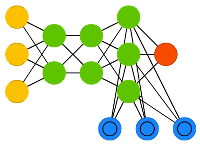
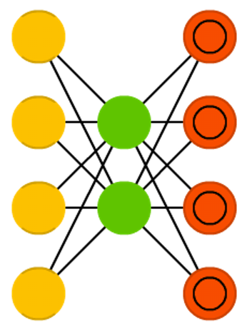
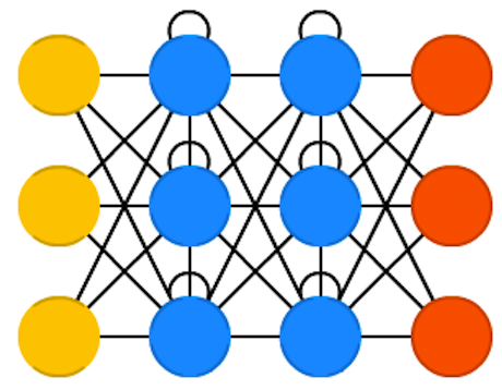
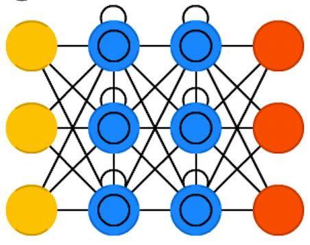
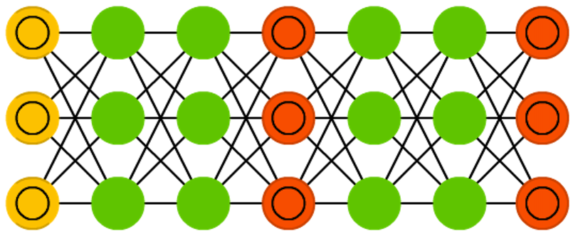
Figure 1 illustrates a number of commonly used structures; for example, feed-forward architectures, auto-encoders, convolutional, and neural Turing machines. Once you have learned the dimensionality of the weight matrices which are non-zero, there’s an implied network structure.

Stacked GLM.

From a statistical viewpoint, deep learning models can be viewed as stacked Generalized Linear Models [Polson and Sokolov, 2017a]. The expectation over dependent variable in GLM is computed using affine transformation (linear regression model) followed by a non-linear univariate function (inverse of the link function). GLM is given by

$$E(y\mid x)=g^{-1}(w^{T}x).$$

Choice of link function is defined by the target distribution $p(y\mid x)$. For example when $p$ is binomial, we choose $g^{-1}$ to be sigmoid $1/(1+\exp(-w^{T}x))$.

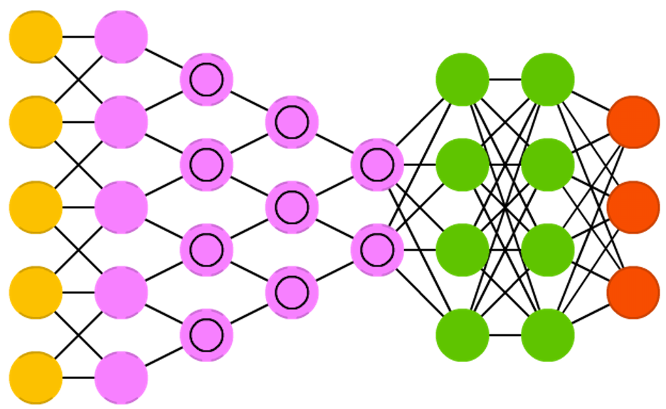Neural Turing Machine	Auto-encoder	Convolution
Recurrent	Long / short term memory	GAN

Figure 1: Commonly used deep learning architectures. Each circle is a neuron which calculates a weighted sum of an input vector plus bias and applies a non-linear function to produce an output. Yellow and red colored neurons are input-output cells correspondingly. Pink colored neurons apply weights inputs using a kernel matrix. Green neurons are hidden ones. Blue neurons are recurrent ones and they append its values from previous pass to the input vector. Blue neuron with circle inside a neuron corresponds to a memory cell. Source: http://www.asimovinstitute.org/neural-network-zoo.

Recently deep architectures (indicating non-zero weights) include convolutional neural networks (CNN), recurrent NN (RNN), long short-term memory (LSTM), and neural Turing machines (NTM). [Pascanu et al., 2013] and [Montúfar and Morton, 2015] provide results on the advantage of representing some functions compactly with deep layers. [Poggio, 2016] extends theoretical results on when deep learning can be exponentially better than shallow learning. [Bryant, 2008] implements [Sprecher, 1972] algorithm to estimate the non-smooth inner link function. In practice, deep layers allow for smooth activation functions to provide “learned” hyper-planes which find the underlying complex interactions and regions without having to see an exponentially large number of training samples.

Commonly used activation functions are sigmoidal ($\cosh$ or $\tanh$), heaviside gate functions $I(x>0)$, or rectified linear units (ReLU) $\max\{\cdot,0\}$. ReLU’s especially have been found [Schmidt-Hieber, 2017] to lend themselves well to rapid dimension reduction. A deep learning predictor is a data reduction scheme that avoids the curse of dimensionality through the use of univariate activation functions. One particular feature is that the weight matrices $W_{l}\in\Re^{N_{l}\times N_{l-1}}$ are matrix valued. This gives the predictor great flexibility to uncover nonlinear features of the data – particularly so in finance data as the estimated hidden features $Z^{(l)}$ can be given the interpretation of portfolios of payouts. The choice of the dimension $N_{l}$ is key, however, since if a hidden unit (aka columns of $W_{l}$) is dropped at layer $l$ it kills all terms above it in the layered hierarchy.

2.2 Autoencoder

An autoencoder is a deep learning routine which trains $F(X)$ to approximate $X$ (i.e., $X=Y$) via a bottleneck structure, which means we select a model $F=f_{l}^{W_{1},b_{1}}\circ\ldots\circ f_{L}^{W_{L},b_{L}}$ which aims to concentrate the information required to recreate $X$. Put differently, an autencoder creates a more cost effective representation of $X$.

For example, for a static autoencoder with two linear layers (a .k.a. traditional factor model), we write

$$Y=W_{1}\left(W_{2}X\right)\,.$$

where $x\in\Re^{k}$ and $W_{hidden}\in\Re^{p\times k}$ and $W_{out}\in\Re^{k\times p}$ where $p\ll k$. The goal of an autoencoder is to train the weights so that $y=x$ with loss function typically given by squared errors.

If $W_{2}$ is estimated from the structure of the training data matrix, then we have a traditional factor model, and the $W_{1}$ matrix provides the factor loadings. We note, that principal component analysis (PCA) in particular falls into this category, as we have seen in (2). If $W_{2}$ is estimated based on the pair $\hat{X}=\{Y,X\}=X$ (which means estimation of $W_{2}$ based on the structure of the training data matrix with the specific autoencoder objective), then we have a sliced inverse regression model. If $W_{1}$ and $W_{2}$ are simultaneously estimated based on the training data $X$, then we have a two layer deep learning model.

A dynamic one layer autoencoder for a financial time series $(Y_{t})$ can, for example, be written as a coupled system of the form

$$Y_{t}=W_{x}X_{t}+W_{y}Y_{t-1}\;\;{\rm and}\;\;\left(\begin{array}[]{c}X_{t}\\ Y_{t-1}\end{array}\right)=WY_{t}\,.$$

We then need to learn the weight matrices $W_{x}$ and $W_{y}$. Here, the state equation encodes and the matrix $W$ decodes the $Y_{t}$ vector into its history $Y_{t-1}$ and the current state $X_{t}$.

The auto encoder demonstrates nicely that in deep learning we do not have to model the variance-covariance matrix explicitly, as our model is already directly in predictive form. (Given an estimated nonlinear combination of deep learners, there is an implicit variance-covariance matrix, but that is not the driver of the method.)

2.3 Factor Models

Almost all shallow data reduction techniques can be viewed as consisting of a low dimensional auxiliary variable $Z$ and a prediction rule specified by a composition of functions

$$\hat{Y} =f_{1}^{W_{1},b_{1}}(f_{2}(W_{2}X+b_{2})\big{)}$$

$$=f_{1}^{W_{1},b_{1}}(Z),\,\text{ where $Z:=f_{2}(W_{2}X+b_{2})$\,. }$$

In this formulation, we also recognise the previously introduced deep learning structure (1). The problem of high dimensional data reduction in general is to find the $Z$-variable and to estimate the layer functions $(f_{1},f_{2})$ correctly. In the layers, we want to uncover the low-dimensional $Z$-structure in a way that does not disregard information about predicting the output $Y$.

Principal component analysis (PCA), reduced rank regression (RRR), linear discriminant analysis (LDA), projection pursuit regression (PPR), and logistic regression are all shallow learners. For example, PCA reduces $X$ to $f_{2}(X)$ using a singular value decomposition of the form

$$Z=f_{2}(X)=W^{\top}X+b\,,$$ (2)

where the columns of the weight matrix $W$ form an orthogonal basis for directions of greatest variance (which is in effect an eigenvector problem). Similarly, for the case of $X=(x_{1},\ldots,x_{p})$, PPR reduces $X$ to $f_{2}(X)$ by setting

$$Z=f_{2}(X)=\sum^{N_{1}}_{i=1}g_{i}(W_{i1}x_{1}+\ldots+W_{ip}x_{p})\,.$$

As stated before, these types of dimension reduction is independent of $y$ and can easily discard information that is valuable for predicting the desired output. Sliced inverse regression (SIR) [Li, 1991] overcomes this drawback somewhat by estimating the layer function $f_{2}$ using data on both, $Y$ and $X$, but still operates independently of $f_{1}$.

Deep learning overcomes many classic drawbacks by jointly estimating $f_{1}$ and $f_{2}$ based on the full training data $\hat{X}=\{Y_{i},X_{i}\}^{T}_{i=1}$, using information on $Y$ and $X$ as well as their relationships, and by using $L>2$ layers. If we choose to use nonlinear layers, we can view a deep learning routine as a hierarchical nonlinear factor model or, more specifically, as a generalised linear model (GLM) with recursively defined nonlinear link functions.

[Diaconis and Shahshahani, 1984] use nonlinear functions of linear combinations. The hidden factors $z_{i}=w_{i1}b_{1}+\ldots+w_{ip}b_{p}$ represents a data reduction of the output matrix $X$. The model selection problem is to choose $N_{1}$ (how many hidden units).

2.4 GANs: Generative Adversarial Networks

GAN has two components – Generator Neural Network and Discriminator Neural Network. The Generator Network $G:z\rightarrow x$ maps random $z$ to a sample from the target distribution $p(x)$ and the Discriminator Network $D(x)$ is a binary classifier with two classes: generated sample and true sample.

We train GAN iteratively by switching between generator and discriminator. This can be represented mathematically as

$$\min_{\theta_{G}}\max_{\theta_{D}}V(D(x\mid\theta_{D}),G(z\mid\theta_{G}))$$

$$V(D,G) =\mathrm{E}_{x\sim p(x)}\left[\log D(x)\right]+\mathrm{E}_{z\sim p(z)}\left[\log(1-D(G(z))\right]$$

In $V(D,G)$, the first term is a deviance that penalizes for misclassification of samples, the goal is to have it close to 1. The second term is entropy that the data from random input (p(z)) passes through the generator, which then generates a fake sample which is then passed through the discriminator to identify the fakeness (aka worst case scenario). In this term, the discriminator tries to maximize it to 0 (i.e. the log probability that the generated data is fake is equal to 0). So overall, the discriminator is trying to maximize our function $V$.

On the other hand, the task of generator is exactly opposite, i.e. it tries to minimize the function $V$ so that the differentiation between real and fake data is a bare minimum. This, in other words is a cat and mouse game between generator and discriminator!

3 Algorithmic Issues

3.1 Training

Let the training dataset be denoted by $\hat{X}=\{Y_{i},X_{i}\}_{i=1}^{T}$. Once the activation functions, size and depth of the learner have been chosen, we need to solve the training problem of finding $(\hat{W},\hat{b})$ where $\hat{W}=(\hat{W}_{1},\ldots,\hat{W}_{L})$ and $\hat{b}=(\hat{b}_{1},\ldots,\hat{b}_{L})$ denote the learning parameters which we compute during training. A more challenging problem, is training the size and depth $N_{l},L$, which is known as the model selection problem. To do this, we need a training dataset $\hat{X}=\{Y_{i},X_{i}\}_{i=1}^{T}$ of input-output pairs, a loss function $l(Y,\hat{Y})$ at the level of the output signal. In its simplest form, we simply solve

$${\rm arg\,min}_{W,b}\frac{1}{N}\sum_{i=1}^{T}l(Y_{i},\hat{Y}(X_{i}))\,,$$ (3)

An $L_{2}$-norm for a traditional least squares problem becomes a suitable error measure, and if we then minimise the loss function $l(Y_{i},\hat{Y}(X_{i}))=\|Y_{i}-\hat{Y}(X_{i})\|^{2}_{2}\,,$ our target function (3) becomes the mean-squared error (MSE).

It is common to add a regularisation penalty $\phi(W,b)$ to avoid over-fitting and to stabilise our predictive rule. We combine this with the loss function with a global parameter $\lambda$ that gauges the overall level of regularisation. We now need to solve

$${\rm arg\,min}_{W,b}\frac{1}{N}\sum_{i=1}^{T}l(Y_{i},\hat{Y}(X_{i}))+\lambda\phi(W,b)\,,$$ (4)

Again we compute a nonlinear predictor $\hat{Y}=\hat{Y}_{\hat{W},\hat{b}}(X)$ of the output $Y$ given the input $X$–the goal of deep learning.

In a traditional probabilistic model $p(Y|\hat{Y}(X))$ that generates the output $Y$ given the predictor $\hat{Y}(X)$, we have the natural loss function $l(Y,\hat{Y})=-\log p(Y|\hat{Y})$ as the negative log-likelihood. For example, when predicting the probability of default, we have a multinomial logistic regression model which leads to a cross-entropy loss function. For multivariate normal models, which includes many financial time series, the $L_{2}$-norm of traditional least squares becomes a suitable error measure.

The common numerical approach for the solution of (4) is a form of stochastic gradient descent, which adapted to a deep learning setting is usually called backpropagation [Rumelhart et al., 1986]. One caveat of backpropagation in this context is the multi-modality of the system to be solved and the resulting slow convergence properties, which is the main reason why deep learning methods heavily rely on the availablility of large computational power.

To allow for cross validation [Hastie et al., 2016] during training, we may split our training data into disjoint time periods of identical length, which is particularly desirable in financial applications where reliable time consistent predictors are hard to come by and have to be trained and tested extensively. Cross validation also provides a tool to decide what levels of regularisation lead to good generalisation (i.e., predictive) rules, which is the classic variance-bias trade-off. A key advantage of cross validation, over traditional statistical metrics such as $t$-ratios and $p$-values, is that we can also use it to assess the size and depth of the hidden layers, that is, solve the model selection problem of choosing $N_{l}$ for $1\leq l\leq L$ and $L$ using the same predictive MSE logic. This ability to seamlessly solve the model selection and estimation problems is one of the reasons for the current widespread use of machine learning methods.

3.1.1 Approximate Inference

The recent successful approaches to develop efficient Bayesian inference algorithms for deep learning networks are based on the reparameterization techniques for calculating Monte Carlo gradients while performing variational inference. Given the data $D=(X,Y)$, the variation inference relies on approximating the posterior $p(\theta\mid D)$ with a variation distribution $q(\theta\mid D,\phi)$, where $\theta=(W,b)$. Then $q$ is found by minimizing the based on the Kullback-Leibler divergence between the approximate distribution and the posterior, namely

$$\text{KL}(q\mid\mid p)=\int q(\theta\mid D,\phi)\log\dfrac{q(\theta\mid D,\phi)}{p(\theta\mid D)}d\theta.$$

Since $p(\theta\mid D)$ is not necessarily tractable, we replace minimization of $\text{KL}(q\mid\mid p)$ with maximization of evidence lower bound (ELBO)

$$\text{ELBO}(\phi)=\int q(\theta\mid D,\phi)\log\dfrac{p(Y\mid X,\theta)p(\theta)}{q(\theta\mid D,\phi)}d\theta$$

The $log$ of the total probability (evidence) is then

$$\log p(D)=\text{ELBO}(\phi)+\text{KL}(q\mid\mid p)$$

The sum does not depend on $\phi$, thus minimizing $\text{KL}(q\mid\mid p)$ is the same that maximizing $\text{ELBO}(q)$. Also, since $\text{KL}(q\mid\mid p)\geq 0$, which follows from Jensen’s inequality, we have $\log p(D)\geq\text{ELBO}(\phi)$. Thus, the evidence lower bound name. The resulting maximization problem $\text{ELBO}(\phi)\rightarrow\max_{\phi}$ is solved using stochastic gradient descent.

To calculate the gradient, it is convenient to write the ELBO as

$$\text{ELBO}(\phi)=\int q(\theta\mid D,\phi)\log p(Y\mid X,\theta)d\theta-\int q(\theta\mid D,\phi)\log\dfrac{q(\theta\mid D,\phi)}{p(\theta)}d\theta$$

The gradient of the first term $\nabla_{\phi}\int q(\theta\mid D,\phi)\log p(Y\mid X,\theta)d\theta=\nabla_{\phi}E_{q}\log p(Y\mid X,\theta)$ is not an expectation and thus cannot be calculated using Monte Carlo methods. The idea is to represent the gradient $\nabla_{\phi}E_{q}\log p(Y\mid X,\theta)$ as an expectation of some random variable, so that Monte Carlo techniques can be used to calculate it. There are two standard methods to do it. First, the log-derivative trick, uses the following identity $\nabla_{x}f(x)=f(x)\nabla_{x}\log f(x)$ to obtain $\nabla_{\phi}E_{q}\log p(Y\mid\theta)$. Thus, if we select $q(\theta\mid\phi)$ so that it is easy to compute its derivative and generate samples from it, the gradient can be efficiently calculated using Monte Carlo methods. Second, we can use the reparametrization trick by representing $\theta$ as a value of a deterministic function, $\theta=g(\epsilon,x,\phi)$, where $\epsilon\sim r(\epsilon)$ does not depend on $\phi$. The derivative is given by

$$\nabla_{\phi}E_{q}\log p(Y\mid X,\theta) =\int r(\epsilon)\nabla_{\phi}\log p(Y\mid X,g(\epsilon,x,\phi))d\epsilon$$

$$=E_{\epsilon}[\nabla_{g}\log p(Y\mid X,g(\epsilon,x,\phi))\nabla_{\phi}g(\epsilon,x,\phi)].$$

The reparametrization is trivial when $q(\theta\mid D,\phi)=N(\theta\mid\mu(D,\phi),\Sigma(D,\phi))$, and $\theta=\mu(D,\phi)+\epsilon\Sigma(D,\phi),~{}\epsilon\sim N(0,I)$. [Kingma and Welling, 2013] propose using $\Sigma(D,\phi)=I$ and representing $\mu(D,\phi)$ and $\epsilon$ as outputs of a neural network (multi-layer perceptron), the resulting approach was called variational auto-encoder. A generalized reparametrization has been proposed by [Ruiz et al., 2016] and combines both log-derivative and reparametrization techniques by assuming that $\epsilon$ can depend on $\phi$.

3.2 Dropout

To avoid overfitting in the training process, dropout is the technique [Srivastava et al., 2014] of removing input dimensions in $X$ randomly with probability $p$. In effect, this replaces the input $X$ by $D\star X$, where $\star$ denotes the element-wise product and $D$ is a matrix of Bernoulli $\mathcal{B}(p)$ random variables. For example, setting $l(Y,\hat{Y})=\|Y-\hat{Y}\|^{2}_{2}$ (to minimise the MSE as explained above) and $\lambda=1$, marginalised over the randomness, we then have a new objective

$${\rm arg\;min}_{W}\;\mathbb{E}_{D\sim{\rm Ber}(p)}\|Y-W(D\star X)\|^{2}_{2}\,,$$

which is equivalent to

$${\rm arg\;min}_{W}\;\|Y-pWX\|^{2}_{2}+p(1-p)\|\Gamma W\|^{2}_{2}\,,$$

where $\Gamma=({\rm diag}(X^{\top}X))^{\frac{1}{2}}$. We can also interpret this last expression as a Bayesian ridge regression with a $g$-prior [Wager et al., 2013]. Put simply, dropout reduces the likelihood of over-reliance on small sets of input data in training.

$${\rm arg\,min}_{W,b}\frac{1}{N_{l}}\sum_{i=1}^{T}l(Y_{i},\hat{Y_{i}})+\lambda\phi(W,b),$$ (5)

Another application of dropout regularisation is the choice of the number of hidden units in a layer (if we drop units of the hidden rather than the input layer and then establish which probability $p$ gives the best results). It is worth recalling though, as we have stated before, that one of the dimension reduction properties of a network structure is that once a variable from a layer is dropped, all terms above it in the network also disappear. This is just the nature of a composite structure for the deep predictor in (1).

3.3 Batch Normalization

Dropout is mostly a technique for regularization. It introduces noise into a neural network to force the neural network to learn to generalize well enough to deal with noise.

Batch normalization [Ioffe and Szegedy, 2015] is mostly a technique for improving optimization. As a side effect, batch normalization happens to introduce some noise into the network, so it can regularize the model a little bit.

We normalize the input layer by adjusting and scaling the activations. For example, when we have features from 0 to 1 and some from 1 to 1000, we should normalize them to speed up learning. If the input layer is benefiting from it, why not do the same thing also for the values in the hidden layers, that are changing all the time, and get 10 times or more improvement in the training speed.

Batch normalization reduces the amount by what the hidden unit values shift around (covariance shift). If an algorithm learned some $X$ to $Y$mapping, and if the distribution of $X$ changes, then we might need to retrain the learning algorithm by trying to align the distribution of $X$ with the distribution of $Y$. Also, batch normalization allows each layer of a network to learn by itself a little bit more independently of other layers. When you have a large dataset, it’s important to optimize well, and not as important to regularize well, so batch normalization is more important for large datasets. You can of course use both batch normalization and dropout at the same time

We can use higher learning rates because batch normalization makes sure that there no extremely high or low activations. And by that, things that previously couldn’t get to train, it will start to train. It reduces overfitting because it has a slight regularization effects. Similar to dropout, it adds some noise to each hidden layers’ activations. Therefore, if we use batch normalization, we will use less dropout, which is a good thing because we are not going to lose a lot of information. However, we should not depend only on batch normalization for regularization; we should better use it together with dropout. How does batch normalization work? To increase the stability of a neural network, batch normalization normalizes the output of a previous activation layer by subtracting the batch mean and dividing by the batch standard deviation.

However, after this shift/scale of activation outputs by some randomly initialized parameters, the weights in the next layer are no longer optimal. SGD ( Stochastic gradient descent) undoes this normalization. Consequently, batch normalization adds two trainable parameters to each layer, so the normalized output is multiplied by a “standard deviation” parameter (gamma) and adds a “mean” parameter (beta). In other words, batch normalization lets SGD do the denormalization by changing only these two weights for each activation, as follows:

$$\mu_{B} =\dfrac{1}{m}\sum_{i=1}^{m}x_{i},~{}~{}\sigma_{B}^{2}=\dfrac{1}{m}\sum_{i=1}^{m}(x_{i}-\mu_{B})^{2}$$

$$\hat{x}_{i} =\dfrac{x_{i}-\mu_{B}}{\sqrt{\sigma_{B}^{2}+\epsilon}},~{}~{}y_{i}=\gamma\hat{x}_{i}+\beta=\mathrm{BN}_{\gamma,\beta}(x_{i}).$$

4 Deep Learning Theory

There are two questions for which we do not yet have a comprehensive and a satisfactory answer. The first is, how to choose a deep learning architecture for a given problem. The second is why the deep learning model does so well on out-of-sample data, i.e. generalize.

To choose an appropriate architecture, from practical point of view, techniques such as Dropout or universal architectures [Kaiser et al., 2017] allow us to spend less time on choosing an architecture. Also some recent Bayesian theory sheds a light on the problem
[Polson and Rockova, 2018]. However, it is still required to go through a trial-and-error process and empirically evaluate large number of models, before an appropriate architecture could be found. On the other hand, there are some theoretical results that shed a light on the architecture choice process.

It was long well known that shallow networks are universal approximators and thus can be used to learn any input-output relations. The first result in this direction was obtained by Kolmogorov [Kolmogorov, 1957] who has shown that any multivariate function can be exactly represented using operations of addition and superposition on univariate functions. Formally, there exist continuous functions $\psi^{pq}$, defined on $[0,1]$ such that each continuous real function $f$ defined on $[0,1]^{n}$ is represented as

$$g(x_{1},\ldots,x_{n})=\sum_{q=1}^{2n+1}\chi_{q}\left(\sum_{p=1}^{n}\psi^{pq}(x_{p})\right),$$

where each $\chi_{q}$ is a continuous real function. This representation is a generalization of earlier results [Kolmogorov, 1956, Arnold, 1963]. In [Kolmogorov, 1956] it was shown that every continuous multivariate function can be represented in the form of a finite superposition of continuous functions of not more than three variables. Later Arnold used that result to solve Hilbert’s thirteenth problem [Arnold, 1963].

However, results of Kolmogorov and Arnold do not have practical application. Their proofs are not constructive and do not demonstrate how functions $\chi$ and $\psi$ can be computed. Further, [Girosi and Poggio, 1989] and references therein show that those functions are not smooth, while in practice smooth functions are used. Further, while functions $\psi$ form a universal basis and do not depend on $g$, the function $\chi$ does depend on the specific form of function $g$. More practical results were obtained by Cybenko [Cybenko, 1989] who showed that a shallow network with sigmoidal activation function can arbitrarily well approximate any continuous function on the $n$-dimensional cube $[0,1]^{n}$. Generalization for a broader class of activation functions was derived in [Hornik, 1991].

Recently, it was shown that deep architectures require smaller number of parameters compared to shallow ones to approximate the same function and thus more computationally viable. It was observed empirically that deep learners perform better. [Montufar et al., 2014] provide some geometric intuition and show that the number of open box regions generated by deep network is much lager than those generated by a shallow one with the same number of parameters. [Telgarsky, 2015] and [Safran and Shamir, 2016] provided specific examples of classes of functions that require an exponential number of parameters as a function of input dimensionality to be approximated by shallow networks.

[Poggio et al., 2017] provides a good overview of results on complexity of shallow and deep networks required to approximate different classes of functions. For example, for shallow (one-layer) network

$$g(x)\approx F(x)=\sum_{i=i}^{N}a_{k}f(w_{k}^{T}x+b_{k})$$

with $f$ being infinitively differentiable and not a polynomial, it is required that $N=\mathcal{O}(\epsilon^{-n/m})$. Here $x\in[0,1]^{n}$ (n-dimensional cube), $g(x)$ is is differentiable up to order $m$ and $\epsilon$ is the required accuracy of the approximation, e.g. $\max_{x}|g(x)-f(x)|<\epsilon$. Thus, the size of neurons required is exponential in the number of input dimensions, i.e. the curse of dimensionality.

Meanwhile, if function $g(x)$ has a special structure, then deep learner avoids the curse of dimensionality problem.

Specifically, let $g(x):R^{n}\rightarrow R$ be a $\mathcal{G}$–function, which is defined as follows. Source nodes are components of the input $x_{1},\ldots,x_{n}$, and there is only one sink node (value of the function. Each node $v$ between the source and sink is a local function of dimensionality $d_{v}<<n$ of low dimensionality and $m_{v}$ times differentiable. For example, in $\mathcal{G}$-function $f(x_{1},\cdots,x_{8})=h_{3}(h_{21}(h_{11}(x_{1},x_{2}),h_{12}(x_{3},x_{4})),h_{22}(h_{13}(x_{5},x_{6}),h_{14}(x_{7},x_{8})))$ each $h$ is “local”, e.g. requires only two-dimensional input to be computed, it has two hidden nodes and each has two inputs ($d_{v}=2$ for every hidden node). The required complexity of deep network to represent such a function is given by

$$N_{s}=\mathcal{O}\left(\sum_{v\in V}\epsilon^{-d_{v}/m_{v}}\right).$$

Thus, when the target function has local structures as defined for a $\mathcal{G}$–function, deep neural networks allow us to avoid curse of dimensionality.

In [Lin et al., 2017] the authors similarly show how the specific structure of the target function to be approximated can be exploited to avoid the curse of dimensionality. Specifically, properties frequently encountered in physics, such as symmetry, locality, compositionality, and polynomial log-probability translate into exceptionally simple neural networks and are shown to lead to low complexity deep network approximators.

The second question of why deep learning models do not overfit and generalize well to out-of-sample data has received less attention in the literature. It was shown in [Zhang et al., 2016] that regularization techniques do not explain a surprisingly good out-of-sample performance. Using a series of empirical experiments it was shown that deep learning models can learn white noise. A contradictory result was obtained in [Liao et al., 2018] and shows that, for a DL model with exponential loss function and appropriately normalized, there is a linear dependence of test loss on training loss.

References

- [Arnold, 1963] Arnold, V. I. (1963). On functions of three variables. Dokl. Akad. Nauk SSSR, 14(4):679–681. [ English translation: American Mathematical Society Translation, 2(28) (1963), pp. 51–-54].
- [Breiman, 2001] Breiman, L. (2001). Statistical Modeling: The Two Cultures (with comments and a rejoinder by the author). Statistical Science, 16(3):199–231.
- [Bryant, 2008] Bryant, D. W. (2008). Analysis of Kolmogorov’s superpostion theorem and its implementation in applications with low and high dimensional data. University of Central Florida.
- [Cybenko, 1989] Cybenko, G. (1989). Approximation by superpositions of a sigmoidal function. Mathematics of control, signals and systems, 2(4):303–314.
- [Diaconis and Shahshahani, 1984] Diaconis, P. and Shahshahani, M. (1984). On Nonlinear Functions of Linear Combinations. SIAM Journal on Scientific and Statistical Computing, 5(1):175–191.
- [Dixon et al., 2017] Dixon, M. F., Polson, N. G., and Sokolov, V. O. (2017). Deep learning for spatio-temporal modeling: Dynamic traffic flows and high frequency trading. arXiv preprint arXiv:1705.09851.
- [Esteva et al., 2017] Esteva, A., Kuprel, B., Novoa, R. A., Ko, J., Swetter, S. M., Blau, H. M., and Thrun, S. (2017). Dermatologist-level classification of skin cancer with deep neural networks. Nature, 542(7639):115–118.
- [Feng et al., 2018a] Feng, G., He, J., and Polson, N. G. (2018a). Deep learning for predicting asset returns. arXiv preprint arXiv:1804.09314.
- [Feng et al., 2018b] Feng, G., Polson, N. G., and Xu, J. (2018b). Deep factor alpha. arXiv preprint arXiv:1805.01104.
- [Girosi and Poggio, 1989] Girosi, F. and Poggio, T. (1989). Representation properties of networks: Kolmogorov’s theorem is irrelevant. Neural Computation, 1(4):465–469.
- [Hastie et al., 2016] Hastie, T., Tibshirani, R., and Friedman, J. (2016). The Elements of Statistical Learning: Data Mining, Inference, and Prediction, Second Edition. Springer, New York, NY, 2nd edition edition.
- [Heaton et al., 2017] Heaton, J., Polson, N., and Witte, J. H. (2017). Deep learning for finance: deep portfolios. Applied Stochastic Models in Business and Industry, 33(1):3–12.
- [Henderson et al., 2017] Henderson, M., Al-Rfou, R., Strope, B., Sung, Y.-h., Lukacs, L., Guo, R., Kumar, S., Miklos, B., and Kurzweil, R. (2017). Efficient natural language response suggestion for smart reply. arXiv preprint arXiv:1705.00652.
- [Hornik, 1991] Hornik, K. (1991). Approximation capabilities of multilayer feedforward networks. Neural networks, 4(2):251–257.
- [Ioffe and Szegedy, 2015] Ioffe, S. and Szegedy, C. (2015). Batch normalization: Accelerating deep network training by reducing internal covariate shift. In International Conference on Machine Learning, pages 448–456.
- [Kadurin et al., 2017] Kadurin, A., Aliper, A., Kazennov, A., Mamoshina, P., Vanhaelen, Q., Khrabrov, K., and Zhavoronkov, A. (2017). The cornucopia of meaningful leads: Applying deep adversarial autoencoders for new molecule development in oncology. Oncotarget, 8(7):10883.
- [Kaiser et al., 2017] Kaiser, L., Gomez, A. N., Shazeer, N., Vaswani, A., Parmar, N., Jones, L., and Uszkoreit, J. (2017). One model to learn them all. arXiv preprint arXiv:1706.05137.
- [Kingma and Welling, 2013] Kingma, D. P. and Welling, M. (2013). Auto-encoding variational Bayes. arXiv preprint arXiv:1312.6114.
- [Kolmogorov, 1956] Kolmogorov, A. N. (1956). On the representation of continuous functions of several variables by superpositions of continuous functions of a smaller number of variables. Dokl. Akad. Nauk SSSR, 108:179–182. [ English translation: American Mathematical Society Translation, 17 (1961), pp. 369–-373].
- [Kolmogorov, 1957] Kolmogorov, A. N. (1957). On the representation of continuous functions of many variables by superposition of continuous functions of one variable and addition. Dokl. Akad. Nauk SSSR, 114(5):953–956. [English translation: American Mathematical Society Translation, 28 (2) (1963), pp. 55–59].
- [Li, 1991] Li, K.-C. (1991). Sliced inverse regression for dimension reduction. Journal of the American Statistical Association, 86(414):316–327.
- [Liao et al., 2018] Liao, Q., Miranda, B., Hidary, J., and Poggio, T. (2018). Classical generalization bounds are surprisingly tight for deep networks. Technical report, Center for Brains, Minds and Machines (CBMM).
- [Lin et al., 2017] Lin, H. W., Tegmark, M., and Rolnick, D. (2017). Why does deep and cheap learning work so well? Journal of Statistical Physics, 168(6):1223–1247.
- [Montúfar and Morton, 2015] Montúfar, G. F. and Morton, J. (2015). When Does a Mixture of Products Contain a Product of Mixtures? SIAM Journal on Discrete Mathematics, 29(1):321–347.
- [Montufar et al., 2014] Montufar, G. F., Pascanu, R., Cho, K., and Bengio, Y. (2014). On the number of linear regions of deep neural networks. In Advances in neural information processing systems, pages 2924–2932.
- [Oord et al., 2016] Oord, A. v. d., Dieleman, S., Zen, H., Simonyan, K., Vinyals, O., Graves, A., Kalchbrenner, N., Senior, A., and Kavukcuoglu, K. (2016). Wavenet: A generative model for raw audio. arXiv preprint arXiv:1609.03499.
- [Pascanu et al., 2013] Pascanu, R., Gulcehre, C., Cho, K., and Bengio, Y. (2013). How to Construct Deep Recurrent Neural Networks. arXiv:1312.6026 [cs, stat]. arXiv: 1312.6026.
- [Poggio, 2016] Poggio, T. (2016). Deep Learning: Mathematics and Neuroscience. A Sponsored Supplement to Science, Brain-Inspired intelligent robotics: The intersection of robotics and neuroscience:9–12.
- [Poggio et al., 2017] Poggio, T., Mhaskar, H., Rosasco, L., Miranda, B., and Liao, Q. (2017). Why and when can deep-but not shallow-networks avoid the curse of dimensionality: a review. International Journal of Automation and Computing, 14(5):503–519.
- [Polson and Rockova, 2018] Polson, N. and Rockova, V. (2018). Posterior concentration for sparse deep learning. arXiv preprint arXiv:1803.09138.
- [Polson and Sokolov, 2017a] Polson, N. G. and Sokolov, V. (2017a). Deep Learning: A Bayesian Perspective. Bayesian Analysis, 12(4):1275–1304.
- [Polson and Sokolov, 2017b] Polson, N. G. and Sokolov, V. O. (2017b). Deep learning for short-term traffic flow prediction. Transportation Research Part C: Emerging Technologies, 79:1–17.
- [Rajpurkar et al., 2017] Rajpurkar, P., Irvin, J., Zhu, K., Yang, B., Mehta, H., Duan, T., Ding, D., Bagul, A., Langlotz, C., Shpanskaya, K., et al. (2017). Chexnet: Radiologist-level pneumonia detection on chest x-rays with deep learning. arXiv preprint arXiv:1711.05225.
- [Ruiz et al., 2016] Ruiz, F. R., AUEB, M. T. R., and Blei, D. (2016). The generalized reparameterization gradient. In Advances in Neural Information Processing Systems, pages 460–468.
- [Rumelhart et al., 1986] Rumelhart, D. E., Hinton, G. E., and Williams, R. J. (1986). Learning representations by back-propagating errors. nature, 323(6088):533.
- [Safran and Shamir, 2016] Safran, I. and Shamir, O. (2016). Depth separation in relu networks for approximating smooth non-linear functions. arXiv preprint arXiv:1610.09887.
- [Schmidt-Hieber, 2017] Schmidt-Hieber, J. (2017). Nonparametric regression using deep neural networks with relu activation function. arXiv preprint arXiv:1708.06633.
- [Shallue and Vanderburg, 2017] Shallue, C. J. and Vanderburg, A. (2017). Identifying exoplanets with deep learning: A five planet resonant chain around kepler-80 and an eighth planet around kepler-90. arXiv preprint arXiv:1712.05044.
- [Sokolov, 2017] Sokolov, V. (2017). Discussion of ‘deep learning for finance: deep portfolios’. Applied Stochastic Models in Business and Industry, 33(1):16–18.
- [Sprecher, 1972] Sprecher, D. A. (1972). A survey of solved and unsolved problems on superpositions of functions. Journal of Approximation Theory, 6(2):123–134.
- [Srivastava et al., 2014] Srivastava, N., Hinton, G. E., Krizhevsky, A., Sutskever, I., and Salakhutdinov, R. (2014). Dropout: a simple way to prevent neural networks from overfitting. Journal of Machine Learning Research, 15(1):1929–1958.
- [Telgarsky, 2015] Telgarsky, M. (2015). Representation benefits of deep feedforward networks. arXiv preprint arXiv:1509.08101.
- [Wager et al., 2013] Wager, S., Wang, S., and Liang, P. S. (2013). Dropout training as adaptive regularization. In Advances in neural information processing systems, pages 351–359.
- [Wojna et al., 2017] Wojna, Z., Gorban, A., Lee, D.-S., Murphy, K., Yu, Q., Li, Y., and Ibarz, J. (2017). Attention-based extraction of structured information from street view imagery. arXiv preprint arXiv:1704.03549.
- [Wu et al., 2016] Wu, Y., Schuster, M., Chen, Z., Le, Q. V., Norouzi, M., Macherey, W., Krikun, M., Cao, Y., Gao, Q., Macherey, K., et al. (2016). Google’s neural machine translation system: Bridging the gap between human and machine translation. arXiv preprint arXiv:1609.08144.
- [Zhang et al., 2016] Zhang, C., Bengio, S., Hardt, M., Recht, B., and Vinyals, O. (2016). Understanding deep learning requires rethinking generalization. arXiv preprint arXiv:1611.03530.