Scaling in the eigenvalue fluctuations of correlation matrices

Abstract

The spectra of empirical correlation matrices, constructed from multivariate data, are widely used in many areas of sciences, engineering and social sciences as a tool to understand the information contained in typically large datasets. In the last two decades, random matrix theory-based tools such as the nearest neighbour eigenvalue spacing and eigenvector distributions have been employed to extract the significant modes of variability present in such empirical correlations. In this work, we present an alternative analysis in terms of the recently introduced spacing ratios, which does not require the cumbersome unfolding process. It is shown that the higher order spacing ratio distributions for the Wishart ensemble of random matrices, characterized by the Dyson index $\beta$, is related to the first order spacing ratio distribution with a modified value of co-dimension $\beta^{\prime}$. This scaling is demonstrated for Wishart ensemble and also for the spectra of empirical correlation matrices drawn from the observed stock market and atmospheric pressure data. Using a combination of analytical and numerics, such scalings in spacing distributions are also discussed.

I Introduction

Large multivariate datasets are commonly encountered in many areas of sciences Wishart1928 ; Kwapien2012 , engineering RMTApplications and social sciences BartholomewBook . Some common examples include the data generated from the financial markets rmt-fin , atmospheric and climate parameters Santhanam2001 and communication networks Barlowe2008 . Analysis of the spectra of empirical correlation matrices constructed from large data sets provides detailed and graded information about the systems being studied. In the last two decades, tools and results from random matrix theory (RMT) have been widely applied to make sense of the information provided by detailed spectra, namely, the eigenvalues and the eigenvectors, of the empirical correlation matrices wilksbook ; jbun . Originally, RMT was conceived as a model for the energy spectra of complex many-body quantum systems such as nuclei and atoms rmt1 ; GuhrReport ; LivanBook . These novel applications of RMT have expanded its scope well outside of its original domain of quantum spectra.

The eigenvalues $E_{i},i=1,2,\ldots,N$ of the empirical correlation matrix of order $N$ are positive definite, i.e., $E_{i}\geq 0$. Typically, the corresponding eigenmodes fall in two broad groups; (i) eigenmodes of the top and bottom few eigenvalues (in magnitude) that carry most of the information embedded in the original dataset (ii) the bulk of rest represents random correlations. It is the latter group that displays a broad agreement with random matrix based results. For instance, the bulk of the correlation matrix spectra obtained from the time series of the largest stocks in the United States, including the ones that make up the S&P index, was shown to be in agreement with the random matrix averages ecm-rmt ; Sitabhra2007 ; Plerou2002 ; Laloux1999 , and some studies have argued that they contain finer correlated structures livan1 ; Kwapien2005 . The density of the bulk of eigenvalues follows Marcenko-Pastur distribution Marcenko67 and can be used to identify the top eigenvalues that carry significant information. The analysis of eigenvectors, in terms of its agreement with Porter-Thomas distribution ptdist , indicates the stocks that are strongly correlated Laloux1999 . A similar approach for the analysis of atmospheric data can distinguish physically relevant modes of atmospheric variability from the those that are noisy Santhanam2001 . By now, many applications akemann2011oxford ; Novembre2008 ; Patterson2006 ; Akemann1997 ; Johansson2000 ranging from biology rmt-bio , image processing fukunaga1990 and network traffic rmt-engg abound.

An often demonstrated property of the bulk of eigenvalues is that the distribution of the spacings $s_{i}=E_{i+1}-E_{i},i=1,2,\dots$, between consecutive eigenvalues (after unfolding) follows the celebrated Wigner distribution, $P(s)=(\pi/2)s\exp(-\pi s^{2}/4)$ rmt1 . This signifies level repulsion, the tendency of the eigenvalues to repel one another. This continues to be a popular test for RMT-like behaviour, especially for the claim that spectral fluctuations of empirical correlation matrices display universal characteristics irrespective of the dataset or system considered for analysis. A major impediment to computing the spacing distribution is the requirement to unfold the eigenvalues, a somewhat unreliable numerical procedure that approximately separates the system dependent eigenvalue properties from the generic ones. This problem can be circumvented by considering the ratio of consecutive spacings, $r_{i}=s_{i+1}/s_{i},i=1,2,\dots$, which are independent of local eigenvalue density and hence does not depend on the system huse ; atas1 ; atas2 . In this work, new scaling properties relating to the distribution of higher order spacings and spacing ratios to the nearest neighbour spacing properties are demonstrated.

The elements of the empirical correlation matrix represent the pair-wise Pearson correlation among the $N$ variables, each one being a time series of length $T$. From the point of view of random matrix theory, correlation matrices fall within the class of Laguerre-Wishart ensemble lwe of random matrix theory represented by $W=D_{R}D_{R}^{S}$, where $D_{R}$ represents the standardized data matrix of order $N$ by $T$ with real, complex or quaternion elements depending on the Dyson index $\beta=1,2,4$ of the ensemble and $X^{S}$ represents self-dual operation on matrix $X$. For the Laguerre-Wishart ensemble indexed by $\beta$ the random matrix average for the spacing ratios is not yet known, though in the limit of matrix size $N\to\infty$, it is well-approximated by that for the Gaussian ensembles given by

$$P(r)=C_{\beta}~{}\frac{(r+r^{2})^{\beta}}{(1+r+r^{2})^{1+\frac{3}{2}\beta}},$$ (1)

where $C_{\beta}$ is a constant whose form is given in Ref.atas2 . However, results for spacing ratios and spacing distributions beyond the nearest neighbours are not yet known. The higher order spacing statistics provide a finer test for the universality of spectral fluctuations. Secondly, the deviations from these will quantify the time-scales up to which random matrix type universality can be expected to be valid in empirical cases. Indeed, long-range correlations such as $\Delta_{3}$ statistics have indicated limitations of RMT assumptions at longer time scales Santhanam2001 ; Plerou2002 ; rmt-engg .

The structure of the paper is as follows: In Sec. II a scaling relation is given for the higher order spacing ratios for the Wishart ensemble of random matrices. In Sec. III, this scaling relation has been tested on various systems which include the spectra of the Wishart random matrix ensembles and the spectra of empirical correlation matrices drawn from the stock market and atmospheric data set. This relation has also been shown to hold good analytically for the first few orders for the spacing distribution. Finally, in Sec. IV this work is summarized and concluded.

Figure 1: The histograms are the $k$-th spacing ratio distribution for the spectra of random Wishart matrix for $\beta=1$ with $N=T=40000$ (a-c), and $N=20000,T=30000$ (d-f). The computed histograms display a good agreement with $P(r,\beta^{\prime})$ shown as solid line. In this, $\beta^{\prime}$ is given by Eq. 4. Inset shows that the minima in $D(\beta^{\prime})$ corresponds to the value of $\beta^{\prime}$ predicted by Eq. 4.

Figure 2: The histograms are the $k$-th spacing ratio distribution for the spectra of random Wishart matrix with (a-c) $\beta=2$ and (d-f) $\beta=4$. For the $N=T$ case, $N=T=20000$; and for $N\neq T$ case, $N=10000$ and $T=20000$. The computed histograms display a good agreement with $P(r,\beta^{\prime})$ shown as solid line ($\beta^{\prime}$ given by Eq. 4).

II Distribution of higher order spacing ratios

Consider a sample correlation matrix $C$ of order $N>>1$, constructed from time series of $N$ variables and each of length $T$, whose ordered eigenvalues are $E_{1}\leq E_{2}\leq\dots\leq E_{N}$. The density of eigenvalues are given, in the limit $T\geq N>>1$, by the Marcenko-Pastur distribution, which predicts an upper and a lower bound for the eigenvalues Marcenko67 . In nearly all of the earlier studies involving spectra of empirical correlation matrices, eigenvalue density and spacing distributions had been widely studied Santhanam2015 . In contrast, in this work, we study the $k$-th order spacing ratios defined by,

$$r_{i}^{(k)} =\frac{s_{i+k}^{(k)}}{s_{i}^{(k)}}=\frac{E_{i+2k}-E_{i+k}}{E_{i+k}-E_{i}},$$ (2)

where $k$-th order spacings can also be defined as $s^{(k)}=s_{i+k}-s_{i}$. If $k=1$, this reduces to the standard nearest neighbour spacing ratio. The distribution of $k$-th order spacing ratio is denoted by $P^{k}(r,\beta)$, where $\beta=1,2,4$ is the co-dimension that represents the Wishart ensemble. Note that the higher order spacing ratios are not uniquely defined atas2 . In Eq. 2 we take them such that no common spacings are shared between the numerator and denominator. Using Eq. 2, the main result of this paper can be stated as follows: for the random matrix of order $N>>1$ and $T\geq N>>1$, from Wishart ensemble with $\beta=1,2$ and 4, the $k$-th order spacing ratio distribution are related to the nearest neighbour $(k=1)$ spacing ratio distribution statistics by

$$P^{k}(r,\beta) =P(r,\beta^{\prime}),~{}~{}~{}~{}~{}\beta=1,2,4,$$ (3)

$$\beta^{\prime} =\frac{k(k+1)}{2}\beta+(k-1),~{}~{}~{}~{}k\geq 1.$$ (4)

In this, $4\leq\beta^{\prime}<\infty$, though for these values of $\beta^{\prime}$ explicit matrix forms for the Wishart ensemble are not known. Though the eigenvalue density given by Marcenko-Pastur distribution depends on the ratio $T/N$ Marcenko67 , the statistics of fluctuations represented by Eq. 4 can be expected to be independent of $T/N$. Similar scaling relation had been postulated for the spacing distribution of Gaussian ensembles porter_abulmagd and its generalizations Forrester2009 , and recently numerical evidence was provided for the ratios Harshini2018a . Both $P^{k}(r,\beta)$ and $P(r,\beta^{\prime})$ have identical functional forms and the modified parameter $\beta^{\prime}$ depends on the order $k$ of the spacing ratio and co-dimension $\beta$. Further, we present strong numerical evidence from Wishart matrices as well as from empirical correlation matrix spectra computed from observed the stock market and atmospheric data.

A rigorous proof of Eqs. (3-4) is mathematically challenging but we give an intuitive argument why $\beta^{\prime}$ should be greater than $\beta$. The eigenvalues of Wishart ensemble has correspondence with the charged particles of a two-dimensional coloumb gas Forresterbook . In this physical picture, the degree of repulsion between eigenvalue pairs beyond the nearest neighbours is greater than that for consecutive eigenvalue pairs. Hence, it appears physically reasonable to expect that $\beta^{\prime}$ for the case of $k>1$ is greater than $\beta$ for $k=1$. For the special case of $k=2$ in the context of circular orthogonal ensemble ($\beta=1$) of RMT, a limited analytical proof was derived in Ref. MehtaDyson . Thus, Eqs.  (3-4) represents a generalization of this result for the spacing ratios of the Wishart ensemble. In the next section we apply the scaling relation in Eqs. (3-4) to the spectra of various systems.

$~{}~{}\beta~{}~{}$	$~{}~{}k~{}~{}$	$~{}~{}\beta^{\prime}~{}~{}$	$\langle r\rangle_{th}$	$\langle r\rangle_{w}$	$\langle r\rangle_{w}$	$\langle r\rangle_{atm}$	$\langle r\rangle_{fin}$
				$(n=m)$	$(n\neq m)$
	2	4	1.174	1.177	1.176	1.214	1.330
1	3	8	1.085	1.086	1.085	1.123	1.237
	4	13	1.052	1.053	1.052	1.089	1.211

Table 1: Mean values of spacing ratio for Wishart matrix $\langle r\rangle_{w}$, atmospheric correlations data $\langle r\rangle_{atm}$ and stock market correlations $\langle r\rangle_{fin}$. The expected theoretical value is $\langle r\rangle_{th}$.

III Results

III.1 Random matrix spectra

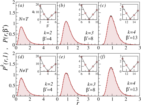
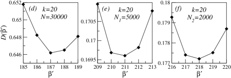
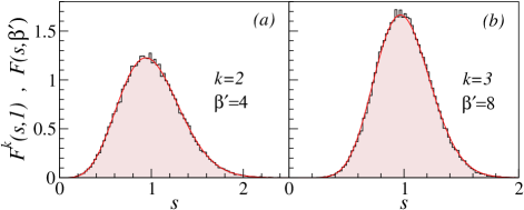
Now, we consider the spectra obtained from an ensemble of Wishart matrices with $\beta=1$ and test the validity of the Eq. 3-4 by computing the higher order spacing ratios. In Fig. 1, the $k$-th order spacing ratio distributions are shown as histograms for two cases, namely, $N=T$ and $N\neq T$. The validity of the scaling in Eq. 3 can be clearly inferred from the excellent agreement of the histogram with a solid curve representing $P(r,\beta^{\prime})$, where $\beta^{\prime}$ given by Eq. 4. An additional layer of quantitative verification can be performed as follows. Let the cumulative distributions corresponding to the computed histogram $P^{k}(r_{i},\beta)$ and $P(r,\beta^{\prime})$ be represented, respectively, by $I^{k}(r_{i},\beta)$ and $I(r_{i},\beta^{\prime})$. In Eq. 4, $\beta^{\prime}$ is treated as a tunable parameter and the difference between cumulative distributions

$$D(\beta^{\prime})=\sum_{i}\left|{I}^{k}(r_{i},\beta)-I(r_{i},\beta^{\prime})\right|,$$ (5)

is computed. The minima of $D(\beta^{\prime})$ is the best value of $\beta^{\prime}$ that fits the histogram data. As seen in the insets in Fig. 1, the minima in $D(\beta^{\prime})$ precisely coincides with the value of $\beta^{\prime}$ postulated in Eq. 4.

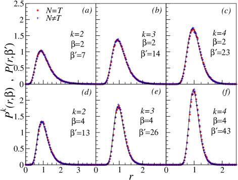
The results displayed in Fig. 2 show that the higher order spacing ratio distributions computed from the spectra from Wishart matrices with $\beta=2$ and 4 are consistent with the scaling relation postulated in Eq. 3-4. The elements of Wishart matrices with $\beta=2$ and 4 are, respectively, complex numbers and quaternions and empirical correlations with such elements are rarely encountered in practice. The symbols in this figure represent the histograms and solid curves represent $P(r,\beta^{\prime})$. The results are shown for both $N=T$ and $N\neq T$ and, as anticipated, the agreement with Eqs. 3-4 is good irrespective of the relative values of $N$ and $T$. Another form of evidence in Table 1 for the mean ratio $\langle r\rangle$ shows a good agreement between the theoretically expected value based on Eqs. 3-4 and that obtained from computed Wishart spectra.

III.2 Stock market and atmospheric data

Next, we demonstrate the validity of the scaling relation Eq. 3-4 for the spectra of empirical correlation matrices drawn from two different domains, namely, the stock market and atmospheric data set. To begin with, the data of the time series of stocks that are part of the S&P500 index for the years 1996-2009 is considered livan1 . This dataset continues to be extensively used to understand the ramifications of how an RMT-based approach might work in the context of empirical correlation matrices. The data consists of daily (log) returns for $T=3400$ days for $N=396$ assets. The elements of the correlation matrix denote the Pearson correlation between pairs of stocks averaged over time. Note that $T\geq N$ implying that the correlations can be assumed to have converged. The statistical properties of its spectra have been reported in Laloux1999 ; ecm-rmt ; Plerou2002 ; Sitabhra2007 .

In Fig. 3(a-c), we display the spacing ratio distribution for various orders. Fig. 3(a) shows the nearest neighbour spacing ratio distribution and it agrees with the analytical result in Eq. 1 obtained for the case of Gaussian Orthogonal Ensemble atas1 . The higher order spacing ratio distributions are displayed in Fig. 3(b,c) and we notice a good agreement with the postulated theoretical distribution $P(r,\beta^{\prime})$, with $\beta^{\prime}$ as given by Eq. 4.

Figure 3: The histograms are the $k$-th order spacing ratio distribution for the spectra of correlation matrix (a-c) from S&P500 stock market data and (d-f) from mean sea level pressure data. The computed histograms display a good agreement with $P(r,\beta^{\prime})$ shown as solid line. In this, $\beta^{\prime}$ is given by Eq. 4.

Figure 4: $D(\beta^{\prime})$ is plotted for $k=11$ (top panel) and $k=20$ (bottom panel) and for (a,d) $N=30000$, (b,e) $N_{1}=5000$, (c,f) $N_{2}=2000$ eigenvalues, for matrices of dimensions $N=T=30000$. $N_{1}$ and $N_{2}$ represent a subset of eigenvalues taken from the bulk of the spectrum.

Figure 5: The histograms are the $k$-th order spacing distribution for the spectra of Wishart matrix. The histograms display a good agreement with $F(s,\beta^{\prime})$ shown as solid line and $\beta^{\prime}$ is given by Eq. 4.

Figure 6: The histograms are the $k$-th spacing distribution for the spectra of correlation matrix (a) from mean sea level pressure data and (b) from S&P500 stock market data. The computed histograms display a good agreement with $F(s,\beta^{\prime})$ shown as solid line and $\beta^{\prime}$ is given by Eq. 4.

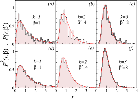
Further, we consider the time series of monthly mean sea level pressure over the north Atlantic ocean. The monthly data is drawn from NCEP reanalysis archives ncep and is available over equally spaced latitude/longitude grids for the North Atlantic region bounded by (0 – 90^o N, 120^o W – 30^o E) for the years 1948 to 2017. Thus, in this case, $N=434$ grid points and $T=840$ months, satisfying the condition $T/N>1$. An analysis of the climate phenomenon of north Atlantic oscillation was performed by constructing an empirical correlation matrix from this data and using RMT statistics such as the spacing and eigenvector distributions Santhanam2001 . In Fig. 3(d), the spacing ratio distributions for the nearest neighbour spacings obtained from the spectra of this correlation matrix is shown. The computed histogram is seen to be well described by the theoretical distribution in Eq. 1 obtained for Gaussian ensembles. The higher order spacing ratio distributions shown in Fig. 3(e-f) display a good agreement with $P(r,\beta^{\prime})$, as anticipated by Eq. 4.

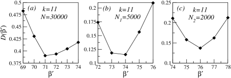
Both these empirical correlation matrix spectra are computed from a relatively short sequence of time series compared to the length of time series used in computing Wishart spectra for Fig. 1. Hence, the noise level for the correlations are higher than for the Wishart case, and it is evident in the higher order spectral statistics shown in Fig. 3. This also manifests as a poor agreement with the $\langle r\rangle$ values shown in Table I. Finally, we point out that violating the conditions, $N>>1$ and $T\geq N\gg 1$, leads to deviations from scaling relation Eqs. 3-4 due to finite size effects as shown in Fig. 4. In the top panel of the figure, it is observed that the minima of $D(\beta^{\prime})$ converges to the predicted value $\beta^{\prime}=76$ on considering a (relatively) small range of eigenvalues in the bulk, where the density of states may be assumed to be constant. This finite size or convergence effect has also been discussed for Gaussian ensembles in Ref. Harshini2018a . While in the bottom panel, it is observed that the minima of $D(\beta^{\prime})$ does not converge to the predicted value $\beta^{\prime}=229$ even on considering a (relatively) small range of eigenvalues in the bulk. To obtain a constant local density of states over a larger energy scale, thus requires a random matrix of larger dimensions.

III.3 Spacing distributions

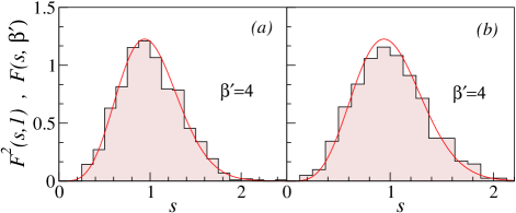
We have also studied the validity of the scaling relation in Eq. 4 for the more popular eigenvalue spacing distribution rmt1 ; Forresterbook . In order to examine this, the $k$-th nearest neighbour spacing is defined as $s^{(k)}=(s_{i+k}-s_{i})/\langle s\rangle,i=1,2,\dots$. Based on the analytical result (see Appendix A) it is postulated that the second (third) order spacing distribution is $F(s,\beta^{\prime})=A_{\beta^{\prime}}s^{\beta^{\prime}}e^{-B_{\beta^{\prime}}s^{2}}$, a form that is reminiscent of the Wigner surmise, where $\beta^{\prime}=3\beta+1$ ($\beta^{\prime}=6\beta+2$). These $\beta^{\prime}$ agrees with Eq. 4 for $k=2$ ($k=3$). The constants $A_{\beta^{\prime}}$ and $B_{\beta^{\prime}}$ depend on $\beta^{\prime}$ and are given in Ref. GuhrReport .

In Fig. 5, we verify this claim for the computed Wishart matrix spectra. The computed histograms display an excellent agreement with the spacing distributions $F(s,\beta^{\prime}=4)$ and $F(s,\beta^{\prime}=8)$ respectively. Fig. 6(a,b) displays next-nearest neighbour ($k=2$) spacing distribution for the data drawn from mean sea level pressure and S&P500 stocks. In both these cases, a good agreement with the anticipated $F(s,\beta^{\prime})$ is evident. For $k>3$, it does not appear straightforward to extend these results due to pronounced finite size effects and the limitations of pushing the spacing distributions postulated based on $s\to 0$ results well beyond its regime of validity.

IV Conclusions

The empirical correlation matrices are widely used in many areas of sciences and engineering as tools to extract information from large datasets. Typically, this is done by analyzing their spectra, the bulk of which are known to follow the random matrix theory predictions, especially for the eigenvalue density and the popular nearest neighbour spacing distribution. Computation of spacing distribution involves unfolding the spectra through an ambiguous fitting procedure. In recent years, the spacing ratio has become a popular alternative to spacing distributions since the former do not depend on the eigenvalue density and hence it does not require unfolding. In this work, for the Wishart matrices of order $N\gg 1$, we focus on the higher order spacing statistics and show that $k$-th order spacing ratio distribution $P^{k}(r,\beta)$ can be obtained in terms of the corresponding nearest neighbour $(k=1)$ distribution, $P(r,\beta^{\prime})$, with $\beta^{\prime}>\beta$, and $\beta^{\prime}$ depends on $k$ and $\beta$. We have used the correspondence of the Wishart eigenvalues with the charged particles of a two-dimensional coloumb gas to explain $\beta^{\prime}>\beta$. Further, using analytical and simulation results, a similar scaling with a limited scope is obtained for the spacing distributions of Wishart matrix spectra and empirical correlation matrices.

We demonstrate the validity of scaling in eigenvalue fluctuations using the spectra drawn from an ensemble of Wishart matrices. As an application with observed datasets, the scaling in fluctuations is also shown for the spectra of empirical correlation matrices obtained from S&P500 stock market data and mean sea level pressure data over North Atlantic ocean, both of these had earlier been analysed from RMT point of view. It would be interesting to obtain these results exactly for the Wishart ensemble. This opens up new tests for the claims of universality of eigenvalue fluctuations and further it can potentially determine the timescales over which RMT-like fluctuations hold good for empirical correlation matrices.

V Acknowledgements

Authors thank Dr Giacomo Livan for providing us S&P 500 correlation matrix data for S&P 500 stocks livan1 , whose eigenvalues are analyzed in this work. UTB acknowledges the funding received from the Department of Science and Technology, India under the scheme Science and Engineering Research Board (SERB) National Post Doctoral Fellowship (NPDF) file number PDF/2015/00050.

Appendix A Spacing distributions for second and third order

In this Appendix the analytical result leading to the second and third order spacing distributions is derived. Consider the random Wishart matrix $W$ of order $N$ and specialized to the case of the next-nearest neighbour $(k=2)$ spacing distribution that can be obtained from Wishart matrix of order $T=3$ with three eigenvalues, $\{E_{1},E_{2},E_{3}\}$. Then, the jpdf of the eigenvalues $E_{l}\geq 0,l=1,2,3$ for the Wishart ensemble is given as follows:

$$f(\{E_{l}\})=\frac{1}{W_{a\beta T}}\prod_{i=1}^{T}E_{i}^{\beta a/2}e^{-\beta E_{i}/2}\prod_{1\leq j<p\leq T}|E_{p}-E_{j}|^{\beta},$$

where $a=N-T+1-2/\beta$ and $W_{a\beta T}$ is a constant Forresterbook . Further, with $T=3$, $N$ and $\beta$ are choosen such that $a=0$. Then, the jpdf can be obtained as,

$$f(E_{1},E_{2},E_{3})=\frac{3!}{W_{0\beta 3}}\prod_{i=1}^{3}e^{-\beta E_{i}/2}\prod_{1\leq j<p\leq 3}|E_{p}-E_{j}|^{\beta}.$$ (6)

Using the transformation $x=E_{2}-E_{1}$, $y=E_{3}-E_{2}$, we obtain $E_{2}=E_{1}+x$, $E_{3}=E_{1}+x+y$ and

$$f(E_{1},x,y)=\frac{3!}{W_{0\beta 3}}x^{\beta}\,y^{\beta}\,(x+y)^{\beta}\,e^{-c\beta(3E_{1}+2x+y)/2}.$$ (7)

Let $K_{1}=3!/W_{0\beta 3}$ and by integrating over $E_{1}$, one obtains

$$f(x,y)=\frac{2K_{1}}{3\beta c}x^{\beta}\,y^{\beta}\,(x+y)^{\beta}e^{-c\beta(2x+y)/2}.$$ (8)

It can be seen that $0\leq x+y=E_{3}-E_{1}=s$ and $y=s-x$. After some algebra, the next-nearest-neighbour $(k=2)$ spacing distribution $\widetilde{F}^{2}(s)$ can be obtained as,

$$\widetilde{F}^{2}(s)=\frac{s^{3\beta+1}e^{-c\beta s/2}}{2^{-1}K_{1}^{-1}3\beta c}\sum_{q=0}^{\beta}\sum_{n=0}^{\infty}{\beta\choose q}\frac{s^{n}(-1)^{\beta-q}(-c\beta/2)^{n}}{n!(2\beta-q+n+1)}\\$$ (9)

In the limit of $s\to 0$, the leading behavior is proportional to $s^{\beta^{\prime}}$, where $\beta^{\prime}=3\beta+1$. The result derived above can be extended easily for the case of $k=3$ as well, resulting in $\beta^{\prime}=6\beta+2$. Thus, based on these analytical results and in the spirit of the scaling relation Eqs. 3-4, it is postulated that the second (third) order spacing distribution is $F(s,\beta^{\prime})=A_{\beta^{\prime}}s^{\beta^{\prime}}e^{-B_{\beta^{\prime}}s^{2}}$ where $\beta^{\prime}=3\beta+1$ ($\beta^{\prime}=6\beta+2$). The constants $A_{\beta^{\prime}}$ and $B_{\beta^{\prime}}$ (given in Ref. GuhrReport ) depend on $\beta^{\prime}$ (Eq. 4).

References

- (1) J. Wishart, Biometrika, 20A , 32 (1928).
- (2) J. Kwapien and S. Drozdz, Phys. Rep. 515, 115 (2012).
- (3) Zhidong Bai, Yang Chen, Ying-Chang Liang, Random Matrix Theory and Its Applications: Multivariate Statistics and Wireless Communications, World Scientific Pub Co Inc. (2009).
- (4) D. J. Bartholomew, F. Steele, J. Galbraith and I. Moustaki Analysis of Multivariate Social Science Data, Chapman and Hall/CRC; London, (2008).
- (5) C. Biely and S. Thurner, Quant. Finance 8, 705 (2008).
- (6) M. S. Santhanam and P. K. Patra, Phys. Rev. E 64, 016102 (2001).
- (7) S. Barlowe, T. Zhang, Y. Liu, J. Yang and D. Jacobs, IEEE Symposium on Proc. VAST’08, 147 (2008).
- (8) J. Bun, J-P. Bouchaud, M. Potters, Phys. Rep. 666, 1 (2017); M. A. Nowak and W. Tarnowsk, J. Stat. Mech. 2017, 063405 (2017).
- (9) S. S. Wilks, Mathematical Statistics, Princeton University Press, New Jersey (1947).
- (10) M. L. Mehta, Random Matrices (Academic Press, New York, 2004).
- (11) T. Guhr, A. Muller-Groeling and H. A. Weidenmüller, Phys. Rep. 299, 189 (1998).
- (12) G. Livan, M. Novaes and P. Vivo, Introduction to Random Matrices : Theory and Practice, (Springer, 2018).
- (13) V. Plerou, P. Gopikrishnan, B. Rosenow, L. A. Nunes Amaral and H. E. Stanley, Phys. Rev. Lett. 83, 1471 (1999).
- (14) L. Laloux, P. Cizeau, J-P Bouchaud, and M. Potters, Phys. Rev. Lett. 83, 1467 (1999).
- (15) V. Plerou, P. Gopikrishnan, B. Rosenow, L. A. Nunes Amaral, T. Guhr, and H. E. Stanley, Phys. Rev. E 65, 066126 (2002).
- (16) Raj Kumar Pan and Sitabhra Sinha, Phys. Rev. E 76, 046116 (2007).
- (17) G. Livan, S. Alfarano and E. Scalas, Phys. Rev. E 84, 016113 (2011).
- (18) J. Kwapien, S. Drozdz, Oswiecimka, Physica A 359, 589 (2006)
- (19) V. A. Marcenko and L. A. Pastur, Math. USSR-Sb 1, 457 (1967).
- (20) C. E. Porter and R. G. Thomas, Phys. Rev. 104, 483 (1956).
- (21) G. Akemann, J. Baik, and P. Di Francesco (eds.), The Oxford handbook of random matrix theory, (Oxford University Press, New York, 2011).
- (22) J. Novembre and M. Stephens, Nature Genetics 40, 646 (2008).
- (23) N. Patterson, A. L. Preis, and D. Reich, PLOS Genetics 2, 2074 (2006).
- (24) G. Akemann, Nucl. Phys. B507, 475 (1997).
- (25) K. Johansson, Comm. Math. Phys. 209 437 (2000).
- (26) P. Śeba, Phys. Rev. Lett. 91, 198104 (2003).
- (27) K. Fukunaga, Introduction to Statistical Pattern Recognition, Elsevier, New York (1990).
- (28) M. Barthélemy, B. Gondran, and E. Guichard, Phys. Rev. E 66, 056110 (2002).
- (29) V. Oganesyan, D. A. Huse, Phys. Rev. B 75, 155111 (2007).
- (30) Y. Y. Atas, E. Bogomolny, O. Giraud, and G. Roux, Phys. Rev. Lett. 110, 084101 (2013).
- (31) Y. Y. Atas et. al., J. Phys. A : Math. Theor. 46, 355204 (2013).
- (32) I. Dumitriu and A. Edelman, J. Math. Phys. 43, 5830 (2002).
- (33) Aashay Patil and M. S. Santhanam, Phys. Rev. E 92, 032130 (2015).
- (34) P. B. Kahn and C. E. Porter, Nucl. Phys. 48, 385 (1963); A. Y. Abul-Magd, and M. H. Simbel, Phys. Rev. E, 60, 5371 (1999).
- (35) P. J. Forrester, Comm. Math. Phys. 285, 653 (2009).
- (36) S. Harshini Tekur, Udaysinh T. Bhosale, M. S. Santhanam, Phys. Rev. B 98, 104305 (2018).
- (37) P. J. Forrester, Log-gases and random matrices, (Princeton University Press, 2010).
- (38) M. L. Mehta and F. J. Dyson, J. Math. Phys. 4, 5 (1963).
- (39) NCEP Reanalysis data provided by the NOAA/OAR/ESRL PSD, Boulder, Colorado, USA, from their web site at www.esrl.noaa.gov/psd/