Boosting algorithms for uplift modeling

Abstract

Uplift modeling is an area of machine learning which aims at predicting the causal effect of some action on a given individual. The action may be a medical procedure, marketing campaign, or any other circumstance controlled by the experimenter. Building an uplift model requires two training sets: the treatment group, where individuals have been subject to the action, and the control group, where no action has been performed. An uplift model allows then to assess the gain resulting from taking the action on a given individual, such as the increase in probability of patient recovery or of a product being purchased. This paper describes an adaptation of the well-known boosting techniques to the uplift modeling case. We formulate three desirable properties which an uplift boosting algorithm should have. Since all three properties cannot be satisfied simultaneously, we propose three uplift boosting algorithms, each satisfying two of them. Experiments demonstrate the usefulness of the proposed methods, which often dramatically improve performance of the base models and are thus new and powerful tools for uplift modeling.

1 Introduction

Machine learning is primarily concerned with the problem of classification, where the task is to predict, based on a number of predictor attributes, the class to which an instance belongs. Unfortunately, classification is not well suited to many problems in marketing or medicine to which it is frequently applied. Consider a direct marketing campaign where potential customers receive a mailing offer. A classifier is typically built based on a small pilot campaign and used to select the customers who should be targeted. As a result, the customers most likely to buy after the campaign will be selected as targets. Unfortunately this is not what a marketer wants. Some of the customers would have bought regardless of the campaign, targeting them resulted in unnecessary costs. Other customers were actually going to make a purchase but were annoyed by the campaign. While, at first sight, such a case may seem unlikely, it is a well known phenomenon in the marketing literature [5, 12]; the result is a loss of a sale or even churn.

We should therefore select customers who will buy because of the campaign, that is, those who are likely to buy if targeted, but unlikely to buy otherwise. Similar problems arise in medicine where some patients may recover without treatment and some may be hurt by treatment’s side effects more than by the disease itself.

Uplift modeling provides a solution to this problem. The approach uses two separate training sets: treatment and control. Individuals in the treatment group have been subjected to the action, those in the control group have not. Instead of modeling class probabilities, uplift modeling attempts to model the difference between conditional class probabilities in the treatment and control groups. This way, the causal influence of the action can be modeled, and the method is able to predict the true gain (with respect to taking no action) from targeting a given individual.

This paper presents an adaptation of boosting to the uplift modeling case. Boosting often dramatically improves performance of classification models, and in this paper we demonstrate that it can bring similar benefits to uplift modeling. We begin by stating three desirable properties of an uplift boosting algorithm. Since all three cannot be satisfied at the same time, we propose three uplift boosting algorithms, each satisfying two of them. Experimental verification proves that the benefits of boosting extend to the case of uplift modeling and shows relative merits of the three algorithms.

We conclude by mentioning a problem which is the biggest challenge of uplift modeling as opposed to standard classification. The problem has been known in statistical literature [7] as the

Fundamental Problem of Causal Inference. For every individual, only one of the outcomes is observed, after the individual has been subject to an action (treated) or when the individual has not been subject to the action (was a control case), never both.

As a result, we never know whether the action performed on a given individual was truly beneficial. This is different from classification, where the true class of each individual in the training set is known.

In the remaining part of this section we describe the notation, give an overview of the related work and review some of the properties of classification boosting.

1.1 Notation and assumptions

We will now introduce the notation used throughout the paper. We use the superscript ^T for quantities related to the treatment group and the superscript ^C for quantities related to the control group. For example, the treatment training dataset will be denoted with ${\cal D}^{T}$ and the control training dataset with ${\cal D}^{C}$. Both datasets together constitute the whole training dataset, ${\cal D}={\cal D}^{T}\cup{\cal D}^{C}$.

Each data record $(x,y)$ consists of a vector of features $x\in\mathcal{X}$ and a class $y\in\{0,1\}$ with $1$ assumed to be the successful outcome, for example patient recovery or a positive response to a marketing campaign. Let $N^{T}$ and $N^{C}$ denote the number of records in the treatment and control datasets.

An uplift model is a function $h:\mathcal{X}\rightarrow\{0,1\}$. The value $h(x)=1$ means the action is deemed beneficial for $x$ by the model, $h(x)=0$ means that its impact is considered neutral or negative. By ‘positive outcome’ we mean that the probability of success for a given individual $x$ is higher if the action is performed on her than if the action is not taken.

We will denote general probabilities related to the treatment and control groups with $P^{T}$ and $P^{C}$, respectively. For example, $P^{T}(y=1,h=1)$ stands for probability that a randomly selected case in the treatment set has a positive outcome and taking the action on it is predicted to be beneficial by an uplift model $h$. We can now state more formally when an individual $x$ should be subject to an action, namely, when $P^{T}(y=1|x)-P^{C}(y=1|x)>0$.

1.2 Related work

Despite its practical appeal, uplift modeling has seen relatively little attention in the literature. A trivial approach is to build two probabilistic classifiers, one on the treatment set, the other on control, and subtract their predicted probabilities. This approach can, however, suffer from a serious drawback: both models may focus on predicting class probabilities themselves, instead of focusing on the, usually much smaller, differences between the two groups. An illustrative example can be found in [12].

Several algorithms have thus been proposed which directly model the difference between class probabilities in the treatment and control groups. Many of them are based on modified decision trees. For example, [12] describe an uplift tree learning algorithm which selects splits based on a statistical test of differences between treatment and control class probabilities. In [14, 15] uplift decision trees based on information theoretical split criteria have been proposed. Since we use those trees as base models, we will briefly discuss the splitting criterion they use.

The splitting criterion for uplift decision trees compares some measure of divergence between treatment and control class probabilities before and after the split. The difference between two probability distributions $P=(p_{1},\ldots,p_{n})$ and $Q=(q_{1},\ldots,q_{n})$ is typically measured using the Kullback-Leibler divergence [1], however the authors found that E-divergence

$$E(P:Q)=\sum_{i}(p_{i}-q_{i})^{2},$$

which is simply the squared Euclidean distance, performed better in the experiments. The test selection criterion (the E-divergence gain) then becomes

$$E_{gain}(A)=\sum_{a\in\mathcal{A}}P(a)E\left(P^{T}(Y|a):P^{C}(Y|a)\right)-E\left(P^{T}(Y):P^{C}(Y)\right),$$

where $\mathcal{A}$ is the set of possible outcomes of the test $A$ and $P(a)$ is a weighted average of probabilities of outcome $a$ in the treatment and control training sets. The value is additionally divided by a penalizing factor which discourages tests with a large number of outcomes or tests which lead to very different splits in the treatment and control training sets. Details can be found in [14, 15].

Some work has also been published on using ensemble methods for uplift modeling, although, to the best of our knowledge, none of them on boosting. Bagging of uplift models has been mentioned in [12]. Uplift Random Forests have been proposed by [3]; an extension, called causal conditional inference trees was proposed by the same authors in [4]. A thorough experimental and theoretical analysis of bagging and random forests in uplift modeling can be found in [18] where it is argued that ensemble methods are especially well suited to this task and that bagging performs surprisingly well.

Other uplift techniques have also been proposed. Regression based approaches can be found in [10] or, in a medical context, in [13, 19]. In [9] a class variable transformation has been proposed, which allows for applying arbitrary classifiers to uplift modeling, however the performance of the method was not satisfactory as it was often outperformed by the double model approach. [8] propose a method for converting survival data such that uplift modeling can, under certain assumptions, be directly applied to it; we will use this method to prepare experimental datasets in Section 4.

Some variations on the uplift modeling theme have also been explored. [11] proposed an approach to online advertising which combines uplift modeling with maximizing the response rate in the treatment group to increase advertiser’s benefits. We do not address such problems in this paper.

1.3 Properties of boosting in the classification case

While many boosting algorithms are available, in this paper by ‘boosting’ we mean the discrete AdaBoost algorithm [2].

We will now briefly summarize two of the properties of boosting in the classification case. The two properties will be important for adapting boosting to the uplift modeling case. Full details can be found for example in [2, 16, 17].

Forgetting the last member.

The first important property is ‘forgetting’ the last model added to the ensemble. After a new member is added, record weights are updated such that its classification error is exactly $1/2$ [17]. This makes it likely for the next member to be very different from the previous one, leading to a diverse ensemble.

Fastest decrease of ensemble’s training error.

It can be shown [2], that training set error of a boosted ensemble is bounded from above by

$$\epsilon\leq 2^{M}\prod_{m=1}^{M}\sqrt{\epsilon_{m}(1-\epsilon_{m})},$$

where $\epsilon_{m}$ is the weighted error of the $m$-th model. The error thus decreases exponentially as long as $\epsilon_{m}<1/2$. Moreover, the updates to record weights as well as the weights of ensemble members are chosen such that this upper bound is minimized.

2 Boosting in the context of uplift modeling

In this section we will present a general uplift boosting algorithm, define an uplift analogue of classification error, and state three properties which uplift boosting algorithms should have.

2.1 A general uplift boosting algorithm

In the $m$-th iteration of the boosting algorithm the $i$-th treatment group training record is assumed to have a weight $w_{m,i}^{T}$ assigned to it. Likewise a weight $w_{m,i}^{C}$ is assigned to the $i$-th control training case. Further, denote by

$$p_{m}^{T}=\frac{\sum_{i=1}^{N^{T}}w_{m,i}^{T}}{\sum_{i=1}^{N^{T}}w_{m,i}^{T}+\sum_{i=1}^{N^{C}}w_{m,i}^{C}},\;\;\;\;\;p_{m}^{C}=\frac{\sum_{i=1}^{N^{C}}w_{m,i}^{C}}{\sum_{i=1}^{N^{T}}w_{m,i}^{T}+\sum_{i=1}^{N^{C}}w_{m,i}^{C}}$$ (1)

the relative sizes of treatment and control datasets at iteration $m$. Notice that $p_{m}^{T}+p_{m}^{C}=1$ for every $m$.

Algorithm 1 presents a general boosting algorithm for uplift modeling. Overall it is similar to boosting for classification but we allow for different weights of records in the treatment and control groups. As a result, model weights $\beta_{m}$ need not be identical to weight rescaling factors $\beta_{m}^{T}$, $\beta^{C}_{m}$.

• set of treatment training records, ${\cal D}^{T}=\{\left(x_{1}^{T},y_{1}^{T}\right),\dots,\left(x_{N^{T}}^{T},y_{N^{T}}^{T}\right)\}$,

• set of control training records, ${\cal D}^{C}=\{\left(x_{1}^{C},y_{1}^{C}\right),\dots,\left(x_{N^{C}}^{C},y_{N^{C}}^{C}\right)\}$,

• base uplift algorithm to be boosted,

• integer $M$ specifying the number of iterations

1. Initialize weights $w_{1,i}^{T},w_{1,i}^{C}$

2. For $m\leftarrow 1,\dots,M$

   1. $w^{T}_{m,i}\leftarrow\frac{w^{T}_{m,i}}{\sum_{j}w^{T}_{m,j}+\sum_{j}w^{C}_{m,j}}$; $w^{C}_{m,i}\leftarrow\frac{w^{C}_{m,i}}{\sum_{j}w^{T}_{m,j}+\sum_{j}w^{C}_{m,j}}$

   2. Build a base model $h_{m}$ on ${\cal D}$ with $w_{m,i}^{T},w_{m,i}^{C}$

   3. Compute the treatment and control errors $\epsilon_{m}^{T}$, $\epsilon_{m}^{C}$

   4. Compute $\beta_{m}^{T}(\epsilon_{m}^{T},\epsilon_{m}^{C})$, $\beta_{m}^{C}(\epsilon_{m}^{T},\epsilon_{m}^{C})$

   5. If $\beta_{m}^{T}=\beta_{m}^{C}=1$ or $\epsilon_{m}^{T}\notin(0,\frac{1}{2})$ or $\epsilon_{m}^{C}\notin(0,\frac{1}{2})$:

      1. choose random weights $w_{m,i}^{T}$, $w_{m,i}^{C}$

      2. continue with next boosting iteration

   6. $w^{T}_{m+1,i}\leftarrow w_{m,i}^{T}\cdot(\beta_{m}^{T})^{1[h_{m}(x_{i}^{T})=y^{T}_{i}]}$

   7. $w^{C}_{m+1,i}\leftarrow w_{m,i}^{C}\cdot(\beta_{m}^{C})^{1[h_{m}(x_{i}^{C})=1-y^{C}_{i}]}$

   8. $\beta_{m}\leftarrow\min\{\beta_{m}^{T},\beta_{m}^{C}\}$

   9. Add $h_{m}$ with coefficient $\beta_{m}$ to the ensemble

Output: The final hypothesis

$$h_{f}(x)=\left\{\begin{array}[]{ll}1&if\;\sum_{m=1}^{M}\left(\log\frac{1}{\beta_{m}}\right)h_{m}(x)\geq\frac{1}{2}\sum_{m=1}^{M}\log\frac{1}{\beta_{m}},\\ 0&otherwise.\end{array}\right.$$ (2)

Algorithm 1 A general uplift boosting algorithm.

The general algorithm leaves many aspects unspecified, such as how record weights are initialized and updated. In fact, several variants of the algorithm are possible. The choice of model weights in step 2h is explained at the end of Section 2.5. In order to pick concrete values of the weight update coefficients we are going to state three desirable properties of an uplift booster and use those properties to derive three different algorithms. The parameters used by those algorithms are summarized in Table 1. The errors $\epsilon^{T}_{m}$ and $\epsilon^{C}_{m}$ are defined in Section 2.2.

Table 1: Coefficient values for the three proposed uplift boosting algorithms.

Algorithm	$\beta_{m}^{T}$	$\beta_{m}^{C}$	weight initialization
uplift AdaBoost	$\frac{p^{T}_{m}\epsilon^{T}_{m}+p^{C}_{m}\epsilon^{C}_{m}}{1-p^{T}_{m}\epsilon^{T}_{m}-p^{C}_{m}\epsilon^{C}_{m}}$		$w^{T}_{1,i},w^{C}_{1,i}\leftarrow 1$
balanced uplift boosting	See Theorem 2		$w^{T}_{1,i}\leftarrow\frac{1}{N^{T}}$; $w^{C}_{1,i}\leftarrow\frac{1}{N^{C}}$
balanced forgeting boosting	$\frac{\epsilon^{C}_{m}}{1-\epsilon^{T}_{m}}$	$\frac{\epsilon^{T}_{m}}{1-\epsilon^{C}_{m}}$	$w^{T}_{1,i}\leftarrow\frac{1}{N^{T}}$; $w^{C}_{1,i}\leftarrow\frac{1}{N^{C}}$

Note that the algorithm is a discrete boosting algorithm [2, 17], that is, the base learners are assumed to return a discrete decision on whether the action should be taken (1) or not (0). Algorithm 1, as presented in the figure, also returns a decision. However, it can also return a numerical score,

$$s(x)=\sum_{m=1}^{M}\left(\log\frac{1}{\beta_{m}}\right)h_{m}(x),$$

indicating how likely it is that the effect of the action is positive on a given case. In the experimental Section 4 we will use this variant of the algorithm.

AdaBoost can suffer from premature stops when the sum of weights of misclassified cases becomes $0$ or is greater than $1/2$. This problem turns to be even more troublesome in the uplift modeling case. Hence, in step 2e of Algorithm 1 we restart the algorithm by assigning random weights drawn from the exponential distribution to records in both training datasets. The technique has been suggested for classification boosting in [20].

Before we proceed to describe the three desirable properties of uplift boosting algorithms we need to define an uplift analogue of classification error.

2.2 An uplift analogue of classification error

Due to the Fundamental Problem of Causal Inference we cannot tell whether an uplift model correctly classified a given instance. We will, however, define an approximate notion of classification error in the uplift case. A record $(x_{i}^{T},y_{i}^{T})$ is assumed to be classified correctly by an uplift model $h$ if $h(x_{i}^{T})=y_{i}^{T}$ and $(x_{i}^{T},y_{i}^{T})\in{\cal D}^{T}$; a record $(x_{i}^{C},y_{i}^{C})$ is assumed to be classified correctly if $h(x_{i}^{C})=1-y_{i}^{C}$ and $(x_{i}^{C},y_{i}^{C})\in{\cal D}^{C}$.

Intuitively, if a record $(x_{i}^{T},y_{i}^{T})$ belongs to the treatment group and a model $h$ predicts that it should receive the treatment ($h(x_{i}^{T})=1$) then the outcome should be positive ($y_{i}^{T}=1$) if the recommendation is to be correct. Note that the gain from the action might also be neutral if a success would have occurred also without treatment, but at least the model’s recommendation is not in contradiction with the observed outcome. If, on the contrary, the outcome for a record in the treatment group is $0$ and $h(x_{i}^{T})=1$, the prediction is clearly wrong as the true effect of the action can at best be neutral.

In the control group the situation is reversed. If the outcome was positive ($y_{i}^{C}=1$) but the model predicted that the treatment should be applied ($h(x_{i}^{C})=1$), the prediction is clearly wrong, since the treatment cannot be truly beneficial, it can at best be neutral. To simplify notation we will introduce the following indicators:

$$e^{T}(x_{i}^{T}) =\begin{cases}0&\mbox{if }x_{i}^{T}\in{\cal D}^{T}\mbox{ and }h(x_{i}^{T})=y_{i}^{T},\cr 1&\mbox{if }x_{i}^{T}\in{\cal D}^{T}\mbox{ and }h(x_{i}^{T})\neq y_{i}^{T},\end{cases}$$ (3)

$$e^{C}(x_{i}^{C}) =\begin{cases}0&\mbox{if }x_{i}^{C}\in{\cal D}^{C}\mbox{ and }h(x_{i}^{C})\neq y_{i}^{C},\cr 1&\mbox{if }x_{i}^{C}\in{\cal D}^{C}\mbox{ and }h(x_{i}^{C})=y_{i}^{C}.\end{cases}$$ (4)

An index $m$ will be added to indicate the $m$-th iteration of the algorithm. Let us now define uplift analogues of classification error on the treatment and control datasets and a combined error:

$$\epsilon_{m}^{T}=\frac{\sum_{i:\;e_{m}^{T}(x_{i})=1}w^{T}_{m,i}}{\sum_{i=1}^{N^{T}}w^{T}_{m,i}},\quad\epsilon_{m}^{C}=\frac{\sum_{i:\;e_{m}^{C}(x_{i})=1}w^{C}_{m,i}}{\sum_{i=1}^{N^{C}}w^{C}_{m,i}},\quad\epsilon_{m}=p_{m}^{T}\epsilon_{m}^{T}+p_{m}^{C}\epsilon_{m}^{C}.$$ (5)

The sums above are a shorthand notation for summing over misclassified instances in the treatment and control training sets, which will also be used later in the paper.

In [9] a class variable transformation was introduced which replaces class values $y_{i}^{C}$ in the control group with their reverses $1-y_{i}^{C}$ while keeping the treatment set class values unchanged. It is easy to see that the errors defined in Equation 5 are equivalent to standard classification errors for the transformed class. According to [9] the method was not very successful in regression settings, but as we will show later in this paper, it can play a useful role in developing uplift boosting algorithms.

We now proceed to introduce the three desirable properties of uplift boosting algorithms.

2.3 Balance

An uplift boosting algorithm is said to satisfy the balance condition if at each iteration $m$

$$\sum_{i=1}^{N^{T}}w_{m,i}^{T}=\sum_{i=1}^{N^{C}}w_{m,i}^{C}.$$ (6)

Due to weight normalization in step 2a the condition can equivalently be stated as $p_{m}^{T}=p^{C}_{m}=\frac{1}{2}$ for all $m$’s. In other words, the total weights assigned to the treatment and control groups remain constant and equal.

The reason balance property may be desirable is to prevent a situation when one of the groups gains much higher weight than the other and, as a result, weak learners focus only on the treatment or control group instead of the differences between them.

Let us now inductively rephrase the condition in terms of an equation on $\beta_{m}^{T}$ and $\beta_{m}^{C}$. For $m=1$ the balance condition can be achieved by proper initialization of weights. Suppose now that it is satisfied at iteration $m$. From Equation (6) and steps 2f and 2g of Algorithm 1 we get, after splitting the sums over correctly and incorrectly classified cases, that to ensure the condition holds at iteration $m+1$, the following equation must be true:

$$\sum_{i:\;e_{m}^{T}(x_{i})=1}w_{m,i}^{T}+\beta_{m}^{T}\sum_{i:\;e_{m}^{T}(x_{i})=0}w_{m,i}^{T}=\sum_{i:\;e_{m}^{C}(x_{i})=1}w_{m,i}^{C}+\beta_{m}^{C}\sum_{i:\;e_{m}^{C}(x_{i})=0}w_{m,i}^{C}.$$

Dividing both sides by $\sum_{i=1}^{N^{T}}w_{m,i}^{T}=\sum_{i=1}^{N^{C}}w_{m,i}^{C}$ and using Equation 5 we get

$$\epsilon_{m}^{T}+\left(1-\epsilon_{m}^{T}\right)\beta_{m}^{T}=\epsilon_{m}^{C}+\left(1-\epsilon_{m}^{C}\right)\beta_{m}^{C},$$

and

$$\beta_{m}^{T}=\frac{\epsilon_{m}^{C}-\epsilon_{m}^{T}}{1-\epsilon_{m}^{T}}+\frac{1-\epsilon_{m}^{C}}{1-\epsilon_{m}^{T}}\beta_{m}^{C}.$$ (7)

Equation 7 holds when $\beta_{m}^{T},\beta_{m}^{C}>0$ and both errors are not equal to $0$ nor $1$ (there must be good and bad cases in both datasets).

2.4 Forgetting the last ensemble member

Let us now examine what the property of forgetting the last model added to the ensemble means in the context of uplift error defined in Equation 5. To forget the member $h_{m}$ added in iteration $m$ we need to choose weights in iteration $m+1$ such that the combined error of $h_{m}$ is exactly one half, $\epsilon_{m}=\frac{1}{2}$. Using a derivation similar to that for the balance condition we see that $\beta_{m}^{T}$ and $\beta_{m}^{C}$ need to satisfy the condition

$$\beta_{m}^{T}\sum_{i:\;e_{m}^{T}(x_{i})=0}w_{m,i}^{T}+\beta_{m}^{C}\sum_{i:\;e_{m}^{C}(x_{i})=0}w_{m,i}^{C}=\sum_{i:\;e_{m}^{T}(x_{i})=1}w_{m,i}^{T}+\sum_{i:\;e_{m}^{C}(x_{i})=1}w_{m,i}^{C},$$ (8)

that is, the total new weights of correctly classified examples need to be equal to total new weights of incorrectly classified examples. After dividing both sides by $\sum_{i=1}^{N^{T}}w_{m,i}^{T}+\sum_{i=1}^{N^{C}}w_{m,i}^{C}$ the equation becomes

$$p^{T}_{m}(1-\epsilon_{m}^{T})\beta_{m}^{T}+p^{C}_{m}(1-\epsilon_{m}^{C})\beta_{m}^{C}=p^{T}_{m}\epsilon_{m}^{T}+p^{C}_{m}\epsilon_{m}^{C}.$$ (9)

Note that unlike classical boosting, this condition does not uniquely determine record weights. Let us now give a justification of this condition in terms of performance of an uplift model.

Theorem 1.

Let $h$ be an uplift model. If the balance condition holds and the assignment of cases to the treatment and control groups is random then the condition that the combined uplift error $\epsilon$ be equal to $\frac{1}{2}$ is equivalent to

$$P(h=1)\left[P^{T}(y=1|h=1)-P^{C}(y=1|h=1)\right]\\ +P(h=0)\left[P^{C}(y=1|h=0)-P^{T}(y=1|h=0)\right]=0.$$ (10)

The proof can be found in Appendix A. Note that the left term in (10) is the total gain in success probability due to the action being taken on cases selected by the model and the right term is the gain from not taking the action on cases not selected by the model. A good uplift model tries to maximize both quantities, so the sum being equal to zero corresponds to a model giving no overall gain over the controls.

When the balance condition holds, the forgetting property thus has a clear interpretation in terms of uplift model performance. When the balance condition does not hold, the interpretation is, at least partially, lost.

2.5 Training error bound

We now derive an upper bound on the uplift analogue to the training error of an ensemble with $M$ members. It is desirable for an uplift algorithm to achieve the fastest possible decrease of this upper bound, or at least to guarantee that the error does not increase as more models are added. We begin by defining the analogue of Equation 5 for the whole ensemble. Let $e_{f}^{T}(x_{i}^{T})$ and $e_{f}^{C}(x_{i}^{C})$ denote the indicators defined in Equations 3 and 4 for the final ensemble $h_{f}$ defined in Equation 2. The errors defined in Equation 5 for $h_{f}$ become

$$\epsilon_{f}^{T}=\frac{\sum_{i:\;e_{f}^{T}(x_{i})=1}w^{T}_{1,i}}{\sum_{i=1}^{N^{T}}w^{T}_{1,i}},\quad\epsilon_{f}^{C}=\frac{\sum_{i:\;e_{f}^{C}(x_{i})=1}w^{C}_{1,i}}{\sum_{i=1}^{N^{C}}w^{C}_{1,i}},\quad\epsilon_{f}=p_{1}^{T}\epsilon_{f}^{T}+p_{1}^{C}\epsilon_{f}^{C}.$$ (11)

Following [2] in this derivation we ignore the weight normalization step 2a of the algorithm since it does not influence the way errors (and consequently scaling factors) are calculated. It only affects step 2b, which has no effect on the derivations below.

Following the derivation from [2] separately for the treatment and control datasets, we obtain

$$\sum_{i=1}^{N^{T}} w_{m+1,i}^{T}+\sum_{i=1}^{N^{C}}w_{m+1,i}^{C}$$

$$\leq\left(\sum_{i=1}^{N^{T}}w_{m,i}^{T}\right)(1-(1-\epsilon_{m}^{T})(1-\beta_{m}^{T}))+\left(\sum_{i=1}^{N^{C}}w_{m,i}^{C}\right)(1-(1-\epsilon_{m}^{C})(1-\beta_{m}^{C}))$$

$$=\sum_{i=1}^{N^{T}}w_{m,i}^{T}+\sum_{i=1}^{N^{C}}w_{m,i}^{C}-(1-\epsilon_{m}^{T})(1-\beta_{m}^{T})\sum_{i=1}^{N^{T}}w_{m,i}^{T}-(1-\epsilon_{m}^{C})(1-\beta_{m}^{C})\sum_{i=1}^{N^{C}}w_{m,i}^{C}$$

$$\leq\left(\sum_{i=1}^{N^{T}}w_{m,i}^{T}+\sum_{i=1}^{N^{C}}w_{m,i}^{C}\right)\left[1-p_{m}^{T}(1-\epsilon_{m}^{T})(1-\beta_{m}^{T})-p_{m}^{C}(1-\epsilon_{m}^{C})(1-\beta_{m}^{C})\right],$$

where the last inequality uses the notation introduced in Equation 1. Applying the inequality $M$ times we get:

$$\sum_{i=1}^{N^{T}}w_{M+1,i}^{T}+\sum_{i=1}^{N^{C}}w_{M+1,i}^{C}\\ \leq\left(\sum_{i=1}^{N^{T}}w_{1,i}^{T}+\sum_{i=1}^{N^{C}}w_{1,i}^{C}\right)\prod_{m=1}^{M}\left[1-p_{m}^{T}(1-\epsilon_{m}^{T})(1-\beta_{m}^{T})-p_{m}^{C}(1-\epsilon_{m}^{C})(1-\beta_{m}^{C})\right].$$ (12)

In order to proceed further, we need to make an additional assumption:

$$\prod_{m=1}^{M}{\beta_{m}^{T}}^{1-e_{m}^{T}(x_{i}^{T})}\geq\prod_{m=1}^{M}{\beta_{m}}^{1-e_{m}^{T}(x_{i}^{T})}\quad\mbox{and}\quad\prod_{m=1}^{M}{\beta_{m}^{C}}^{1-e_{m}^{C}(x_{i}^{C})}\geq\prod_{m=1}^{M}{\beta_{m}}^{1-e_{m}^{C}(x_{i}^{C})},$$

respectively for all $x_{i}^{T}$, $x_{i}^{C}$. Recall that $\beta_{m}$ is the weight of $m$-th ensemble member and $\beta_{m}^{T},\beta_{m}^{C}$ the scaling factors for record weights. Notice that this assumption is implied by

$$\beta_{m}^{T}\geq\beta_{m},\;\;\;\;\;\beta_{m}^{C}\geq\beta_{m},$$ (13)

which is stronger, but easier to use in practice.

The final boosting ensemble with $M$ members makes a mistake on $x_{i}^{T}\in{\cal D}^{T}$, the $i$-th training instance of the treatment dataset (respectively the $i$-th control instance, $x_{i}^{C}\in{\cal D}^{C}$) only if [2]

$$\prod_{m=1}^{M}\left(\beta_{m}\right)^{-e_{m}^{T}(x_{i}^{T})}\geq\left(\prod_{m=1}^{M}\beta_{m}\right)^{-\frac{1}{2}}\qquad\mbox{and}\qquad\prod_{m=1}^{M}\left(\beta_{m}\right)^{-e_{m}^{C}(x_{i}^{C})}\geq\left(\prod_{m=1}^{M}\beta_{m}\right)^{-\frac{1}{2}}.$$ (14)

Notice also that the final weights of an instance $x_{i}\in{\cal D}^{T}$ and $x_{i}\in{\cal D}^{C}$ are, respectively,

$$w_{M+1,i}^{T}=w_{1,i}^{T}\prod_{m=1}^{M}\left(\beta_{m}^{T}\right)^{1-e_{m}^{T}(x_{i}^{T})}\quad\mbox{and}\quad w_{M+1,i}^{C}=w_{1,i}^{C}\prod_{m=1}^{M}\left(\beta_{m}^{C}\right)^{1-e_{m}^{C}(x_{i}^{C})},$$

where $w_{1,i}^{T}$ and $w_{1,i}^{C}$ are initial weights set in step 1 of the algorithm. Now we can combine the above equations to bound the error $\epsilon_{f}=p_{1}^{T}\epsilon_{f}^{T}+p_{1}^{C}\epsilon_{f}^{C}$:

$$\sum_{i=1}^{N^{T}}w_{M+1,i}^{T} +\sum_{i=1}^{N^{C}}w_{M+1,i}^{C}\geq\sum_{i:\;e_{f}^{T}(x_{i})\neq 0}w_{M+1,i}^{T}+\sum_{i:\;e_{f}^{C}(x_{i})\neq 0}w_{M+1,i}^{C}$$

$$=\sum_{i:\;e_{f}^{T}(x_{i})\neq 0}w_{1,i}^{T}\prod_{m=1}^{M}\left(\beta_{m}^{T}\right)^{1-e_{m}^{T}(x_{i})}+\sum_{i:\;e_{f}^{C}(x_{i})\neq 0}w_{1,i}^{C}\prod_{m=1}^{M}\left(\beta_{m}^{C}\right)^{1-e_{m}^{C}(x_{i})}$$

$$\geq\sum_{i:\;e_{f}^{T}(x_{i})\neq 0}w_{1,i}^{T}\prod_{m=1}^{M}\left(\beta_{m}\right)^{1-e_{m}^{T}(x_{i})}+\sum_{i:\;e_{f}^{C}(x_{i})\neq 0}w_{1,i}^{C}\prod_{m=1}^{M}\left(\beta_{m}\right)^{1-e_{m}^{C}(x_{i})}$$

$$\geq\left(\prod_{m=1}^{M}\beta_{m}\right)^{\frac{1}{2}}\left(\sum_{i:\;e_{f}^{T}(x_{i})\neq 0}w_{1,i}^{T}+\sum_{i:\;e_{f}^{C}(x_{i})\neq 0}w_{1,i}^{C}\right)$$

The second inequality follows from Equation 13 and the last one was obtained using Equation 14. Combining with Inequality 12 we obtain

$$\prod_{m=1}^{M}\frac{1-p_{m}^{T}(1-\epsilon_{m}^{T})(1-\beta_{m}^{T})-p_{m}^{C}(1-\epsilon_{m}^{C})(1-\beta_{m}^{C})}{\left(\beta_{m}\right)^{\frac{1}{2}}}\geq p_{1}^{T}\epsilon_{f}^{T}+p_{1}^{C}\epsilon_{f}^{C}=\epsilon_{f},$$ (15)

an upper bound for resubstitution error of the final hypothesis on datasets ${\cal D}^{T}$, ${\cal D}^{C}$.

Note that for fixed $\beta_{m}^{T}$ and $\beta_{m}^{C}$, the bound is optimized (subject to the constraint given in Equation 13) by choosing $\beta_{m}=\min\{\beta_{m}^{T},\beta_{m}^{C}\}$. This is the rationale for step 2h of Algorithm 1.

3 Uplift boosting algorithms

In the previous section we introduced three properties which uplift boosting algorithms should satisfy. Unfortunately, as will soon become apparent, all three cannot be satisfied by a single algorithm. Therefore, in this section we will derive three uplift boosting algorithms, each satisfying two of the properties.

3.1 Uplift AdaBoost

We begin with uplift AdaBoost, an algorithm obtained by optimizing the upper bound on the training error given in Equation 15. The optimization will proceed iteratively for $m=1,\ldots,M$; in the $m$-th iteration we minimize the expression

$$\frac{1-p_{m}^{T}(1-\epsilon_{m}^{T})(1-\beta_{m}^{T})-p_{m}^{C}(1-\epsilon_{m}^{C})(1-\beta_{m}^{C})}{\sqrt{\beta_{m}}}$$ (16)

over $\beta_{m}^{T},\beta_{m}^{C}$ with $\epsilon_{m}^{T},\epsilon_{m}^{C}$ fixed. Notice that, while minimizing this expression, we need to respect the constraint given in Equation 13. Suppose the expression is minimized by some $\beta_{m}^{T*}$, $\beta_{m}^{C*}$, $\beta_{m}^{*}$, with $\beta_{m}^{*T}>\beta_{m}^{*}$. However, the numerator of the fraction above is an increasing function of $\beta_{m}^{T}$ and $\beta_{m}^{C}$ for $\beta_{m}$ fixed. Therefore we could replace $\beta_{m}^{T*}$ with $\beta_{m}^{*}$ to obtain a better solution. Analogous argument holds for $\beta_{m}^{C}$. We can conclude that an optimal solution must satisfy $\beta_{m}^{T*}=\beta_{m}^{C*}=\beta_{m}^{*}$, that is, treatment, control and model weights need to be equal. Taking this equality into account, Equation 16 can be simplified to

$$\frac{1-\left[1-(p_{m}^{T}\epsilon_{m}^{T}+p_{m}^{C}\epsilon_{m}^{C})\right](1-\beta_{m})}{\sqrt{\beta_{m}}},$$ (17)

very similar to the one obtained by [2]. Taking the derivative and equating to zero we obtain the optimal $\beta_{m}$:

$$\beta_{m}^{*}=\frac{p_{m}^{T}\epsilon_{m}^{T}+p_{m}^{C}\epsilon_{m}^{C}}{1-\left(p_{m}^{T}\epsilon_{m}^{T}+p_{m}^{C}\epsilon_{m}^{C}\right)}.$$ (18)

This result is identical to classical boosting with the classification error replaced by its uplift analogue. In fact, the algorithm is identical to an application of AdaBoost with class variable transformation from [9]. Here we prove that it is in a certain sense optimal.

At each iteration the upper bound is multiplied by

$$2\sqrt{(p_{m}^{T}\epsilon_{m}^{T}+p_{m}^{C}\epsilon_{m}^{C})(1-\left(p_{m}^{T}\epsilon_{m}^{T}+p_{m}^{C}\epsilon_{m}^{C}\right))}.$$

It is easy to see that the bound cannot increase as more members are added to the ensemble and does in fact decrease, as long as $p_{m}^{T}\epsilon_{m}^{T}+p_{m}^{C}\epsilon_{m}^{C}\neq\frac{1}{2}$.

Let us now look into the two remaining properties. Using $\beta_{m}^{T}=\beta_{m}^{C}=\beta_{m}$, Equation 9 can be rewritten as

$$1-(p^{T}_{m}\epsilon_{m}^{T}+p^{C}_{m}\epsilon_{m}^{C})=\frac{p^{T}_{m}\epsilon_{m}^{T}+p^{C}_{m}\epsilon_{m}^{C}}{\beta_{m}}.$$

Substituting Equation 18 proves that the forgetting property is satisfied by this algorithm.

Note, however, that the balance property need not be satisfied. There is therefore a risk that the method may focus on only one of the groups: treatment or control, reducing the weights of records in the other group to insignificance. Moreover, the uplift interpretation of the forgetting property given in Theorem 1 is no longer valid.

3.2 Balanced uplift boosting

Uplift AdaBoost presented in Section 3.1 may suffer from imbalance between the treatment and control training sets. In this section we will develop the balanced uplift boosting algorithm which optimizes the error bound given in Equation 15 under the constraint that the balance condition holds. Let us first define constants $a_{m}$ and $b_{m}$ to write Equation 7 in a more concise form:

$$\beta_{m}^{T}=\underbrace{\frac{\epsilon_{m}^{C}-\epsilon_{m}^{T}}{1-\epsilon_{m}^{T}}}_{b_{m}}+\underbrace{\frac{1-\epsilon_{m}^{C}}{1-\epsilon_{m}^{T}}}_{a_{m}}\beta_{m}^{C}=a_{m}\beta_{m}^{C}+b_{m}.$$ (19)

Substituting into Equation 16 we get a new bound on error decrease in iteration $m$ which takes into account the balance condition:

$$f\left(\beta_{m}^{C}\right)=\frac{1-(1-\epsilon_{m}^{C})(1-\beta_{m}^{C})}{\sqrt{\beta_{m}}}.$$

Using the assumption $\beta_{m}\leq\min\{\beta_{m}^{T},\beta_{m}^{C}\}$ given in Equation 13 and the fact that $f$ is a decreasing function of $\beta_{m}$ we get that, at optimum, $\beta_{m}=\min\{\beta_{m}^{T},\beta_{m}^{C}\}$. The bound becomes

$$f\left(\beta_{m}^{C}\right)=\frac{1-(1-\epsilon_{m}^{C})(1-\beta_{m}^{C})}{\sqrt{\min\{\beta_{m}^{C},a_{m}\beta_{m}^{C}+b_{m}\}}}.$$ (20)

Minimizing this bound we obtain the value of $\beta_{m}^{C}$; $\beta_{m}^{T}$ is then computed from Equation 19. The optimal value of $\beta_{m}^{C}$ is given by the following theorem.

Theorem 2.

The bound in Equation 20 is minimized for

$$\operatorname*{arg\,min}_{\beta_{m}^{C}\in(0,+\infty)}f(\beta_{m}^{C})=\left\{\begin{array}[]{ll}\frac{2\epsilon_{m}^{T}-\epsilon_{m}^{C}}{1-\epsilon_{m}^{C}}&if\;\epsilon_{m}^{C}<\epsilon_{m}^{T}<\frac{1}{2}\;or\;\frac{1}{2}<\epsilon_{m}^{T}<\epsilon_{m}^{C},\\ \frac{\epsilon_{m}^{C}}{1-\epsilon_{m}^{C}}&if\;\epsilon_{m}^{T}<\epsilon_{m}^{C}<\frac{1}{2}\;or\;\frac{1}{2}<\epsilon_{m}^{C}<\epsilon_{m}^{T},\\ 1&otherwise,\end{array}\right.$$ (21)

and the corresponding minimum is

$$\min_{\beta_{m}^{C}\in(0,+\infty)}f(\beta_{m}^{C})=\left\{\begin{array}[]{ll}2\sqrt{\epsilon_{m}^{T}(1-\epsilon_{m}^{T})}&if\;\epsilon_{m}^{C}<\epsilon_{m}^{T}<\frac{1}{2}\;or\;\frac{1}{2}<\epsilon_{m}^{T}<\epsilon_{m}^{C},\\ 2\sqrt{\epsilon_{m}^{C}(1-\epsilon_{m}^{C})}&if\;\epsilon_{m}^{T}<\epsilon_{m}^{C}<\frac{1}{2}\;or\;\frac{1}{2}<\epsilon_{m}^{C}<\epsilon_{m}^{T},\\ 1&otherwise.\end{array}\right.$$ (22)

See Appendix B for the proof. This result is easy to interpret. Suppose that $\epsilon_{m}^{T}<\epsilon_{m}^{C}<\frac{1}{2}$. We take the larger of the two training errors, $\epsilon^{C}_{m}$, reweight the control dataset using classical boosting weight update and reweight the treatment dataset such that the balance condition is maintained. If $\epsilon_{m}^{C}<\epsilon_{m}^{T}<\frac{1}{2}$ the situation is symmetrical. The decrease in upper bound (Equation 22) is interpreted as follows: compute the decrease rate of standard AdaBoost separately based on the treatment and control errors. Then take the larger (i.e. worse) of the two factors.

Note that we are guaranteed that the bound will actually decrease only when $\epsilon_{m}^{T},\epsilon_{m}^{C}$ lie on the same side of $\frac{1}{2}$, a much stricter condition than for uplift AdaBoost. In any case we are, however, guaranteed that the bound will not increase when another model is added to the ensemble.

Note also, that balanced uplift boosting does not, in general, have the property of forgetting the last member added to the ensemble. This is an immediate consequence of the derivations in the next section.

3.3 Balanced forgetting boosting

We now present another uplift boosting algorithm satisfying different properties, namely the balance condition and forgetting of the last added member. We assume that at the $m$-th iteration the balance condition is satisfied, $p^{T}_{m}=p^{C}_{m}=\frac{1}{2}$. We want to pick factors $\beta^{T}_{m}$, $\beta^{C}_{m}$ such that in the next iteration the balance condition continues to hold and the current model is ‘forgotten’, that is, its error is exactly one half. Since $p^{T}_{m}=p^{C}_{m}=\frac{1}{2}$, Equation 9 can be rewritten as

$$\beta_{m}^{T}=\frac{\epsilon_{m}^{T}+\epsilon_{m}^{C}}{1-\epsilon_{m}^{T}}-\frac{1-\epsilon_{m}^{C}}{1-\epsilon_{m}^{T}}\beta_{m}^{C},$$ (23)

which, after adding to Equation 7, gives $\beta_{m}^{T}=\frac{\epsilon_{m}^{C}}{1-\epsilon_{m}^{T}}$. Analogously, $\beta_{m}^{C}=\frac{\epsilon_{m}^{T}}{1-\epsilon_{m}^{C}}$. We still need to choose $\beta_{m}$. Since the bound in Equation 16 is a decreasing function of $\beta_{m}$ we set it to $\min\{\beta_{m}^{T},\beta_{m}^{C}\}$, the highest value satisfying Inequality 13. Note that the upper bound on the error need no longer be optimal; let us compute it explicitly.

First, we provide a condition for $\beta_{m}^{T}<\beta_{m}^{C}$ or equivalently $\frac{\epsilon_{m}^{C}}{1-\epsilon_{m}^{T}}<\frac{\epsilon_{m}^{T}}{1-\epsilon_{m}^{C}}$. After multiplying, the second inequality becomes $\epsilon_{m}^{C}(1-\epsilon_{m}^{C})<\epsilon_{m}^{T}(1-\epsilon_{m}^{T})$, which is true when $\epsilon_{m}^{C}$ is further from $\frac{1}{2}$ than $\epsilon_{m}^{T}$. Assume now $\epsilon_{m}^{C}<\epsilon_{m}^{T}<\frac{1}{2}$, so $\beta_{m}^{T}<\beta_{m}^{C}$; the remaining cases are analogous and are thus omitted. After substitution of the expressions for $\beta_{m}^{T}$ and $\beta_{m}^{C}$ into Equation 16 we get

$$\frac{1-p_{m}^{T}(1-\epsilon_{m}^{T})(1-\frac{\epsilon_{m}^{C}}{1-\epsilon_{m}^{T}})-p_{m}^{C}(1-\epsilon_{m}^{C})(1-\frac{\epsilon_{m}^{T}}{1-\epsilon_{m}^{C}})}{\sqrt{\frac{\epsilon_{m}^{C}}{1-\epsilon_{m}^{T}}}}=\sqrt{\frac{1-\epsilon_{m}^{T}}{\epsilon_{m}^{C}}}(\epsilon_{m}^{T}+\epsilon_{m}^{C}).$$

Notice that the balanced forgetting boosting algorithm does not guarantee that the error bound will decrease at all: with $\epsilon^{T}$ constant and $\epsilon^{C}$ tending to zero, the bound becomes infinite. It is thus possible that the algorithm will diverge when more members are added to the ensemble.

Let us now compare the bound with that of the balanced uplift boosting algorithm. When $\epsilon_{m}^{C}<\epsilon_{m}^{T}<\frac{1}{2}$ its error bound is $2\sqrt{\epsilon_{m}^{T}(1-\epsilon_{m}^{T})}$. From $(\sqrt{\epsilon_{m}^{T}}-\sqrt{\epsilon_{m}^{C}})^{2}\geq 0$ it follows that $\epsilon_{m}^{T}+\epsilon_{m}^{C}\geq 2\sqrt{\epsilon_{m}^{T}}\sqrt{\epsilon_{m}^{C}}$ giving

$$\sqrt{1-\epsilon_{m}^{T}}\frac{\epsilon_{m}^{T}+\epsilon_{m}^{C}}{\sqrt{\epsilon_{m}^{C}}}\geq\sqrt{1-\epsilon_{m}^{T}}\frac{2\sqrt{\epsilon_{m}^{T}}\sqrt{\epsilon_{m}^{C}}}{\sqrt{\epsilon_{m}^{C}}}=2\sqrt{(1-\epsilon_{m}^{T})\epsilon_{m}^{T}}.$$

The other cases for which $\epsilon_{m}^{T},\epsilon_{m}^{C}$ lie on the same side of $\frac{1}{2}$ are analogous. In those cases balanced uplift boosting always gives stronger guarantees on the decrease of the training set error. If, however, $\epsilon_{m}^{T},\epsilon_{m}^{C}$ lie on the opposite sides of $\frac{1}{2}$, the comparison can go either way.

4 Experimental evaluation

In this section we present an experimental evaluation of the three proposed algorithms and compare their performance with performance of the base models and bagging. We begin by describing the test datasets we are going to use, then review the approaches to evaluating uplift models and finally present the experimental results.

4.1 Benchmark data sets

Unfortunately, not many datasets involving true control groups obtained through randomized experiments are publicly available. We have used one marketing dataset and a few datasets from controlled medical trials, see Table 2 for a summary.

Table 2: Datasets from randomized trials used in the paper.

		#records			#attri-
dataset	source	treatment	control	total	butes
Hillstrom visit	MineThatData blog	21,306	21,306	42,612	8
	[6]
burn	R, KMsurv package	84	70	154	17
hodg	R, KMsurv package	16	27	43	7
bladder	R, survival package	38	47	85	6
colon death	R, survival package	614	315	929	14
colon recurrence	R, survival package	614	315	929	14
veteran	R, survival package	69	68	137	9

The marketing dataset comes from Kevin Hillstrom’s MineThatData blog [6] and contains results of an e-mail campaign for an Internet retailer. The dataset contains information about 64,000 customers who have been randomly split into three groups: the first received an e-mail campaign advertising men’s merchandise, the second a campaign advertising women’s merchandise, and the third was kept as a control. Data is available on whether a person visited the website and/or made a purchase (conversion). We only use data on visits since very few conversions actually occurred. In this paper we use only the treatment group which received women’s merchandise campaign because this group was, overall, much more responsive.

The six medical datasets, based on real randomized trials, come from the survival and kmsurv packages in the R statistical system. Their descriptions are readily available online and are thus omitted. The colon dataset involves two possible treatments and a control. We have kept only one of the treatments (levamisole), the other (levamisole+5fu) was beneficial for all patients and targeting specific groups brought no improvement. All those datasets contain survival data and require preprocessing before uplift boosting can be applied. [8] proposed a simple conversion method where some threshold $\theta$ is chosen and cases for which the observed (possibly censored) survival time is at least $\theta$ are considered positive outcomes, the remaining ones negative. The authors demonstrate that, under reasonable assumptions, an uplift model trained on such data will indeed make correct recommendations even though censoring is ignored. Here we pick the threshold $\theta$ to be the median observed survival time in the dataset.

4.2 Methodology

In this section we discuss the evaluation of uplift models which is more difficult than evaluating traditional classifiers due to the Fundamental Problem of Causal Inference mentioned in Section 1. For a given individual we only know the outcome after treatment or without treatment, never both. As a result, we never know whether the action taken on a given individual has been truly beneficial. Therefore, we cannot assess model performance at the level of single objects, this is possible only for groups of objects. Usually such groups are compared based on an assumption that objects which are assigned similar scores by an uplift model are indeed similar and can be compared with each other.

To assess performance of uplift models we will use so called uplift curves [12, 14]. Notice that since building uplift models requires two training sets, we now also have two test sets: treatment and control. Recall that one of the tools for assessing performance of standard classifiers are lift curves, where the $x$ axis corresponds to the number of cases subjected to an action and the $y$ axis to the number of successes captured. In order to obtain an uplift curve we score both test sets using the uplift model and subtract the lift curve generated on the control test set from the lift curve generated on the treatment test set. The number of successes for both curves is expressed as percentage of the total population such that the subtraction is meaningful.

The interpretation of an uplift curve is as follows: on the $x$ axis we select the percentage of the population on which the action is performed and on the $y$ axis we read the net gain in success probability (with respect to taking no action) achieved on the targeted group. The point at $x=100\%$ gives the gain that would have been obtained if the action was applied to the whole population. The diagonal corresponds to targeting a randomly selected subset. Example curves are shown in Section 4.3, more details can be found in [14, 12].

As with ROC curves, we can use the Area Under the Uplift Curve (AUUC) to summarize model performance with a single number. In this paper we subtract the area under the diagonal from this value to obtain more meaningful numbers. Note that AUUC can be less than zero; this happens when the model gives high scores to cases for which the action has a predominantly negative effect.

The experiments have been performed by randomly splitting both treatment and control datasets into train (80%) and test (20%) parts. The process has been repeated 256 times and the results averaged to improve repeatability of the experiments.

4.3 Experiments

We will now present the experimental results. As base models we are going to use two types of unpruned E-divergence based uplift trees: stumps (trees of height one) and trees of height three with eight leaves (assuming binary splits). See Section 1 and [14] for more details.

Recall from Section 2.1 that our boosting algorithms are discrete, that is ensemble members return 0-1 predictions, not numerical scores, however, bagging and boosting algorithms themselves do produce numerical scores. Since the base models can, in principle, also return numerical scores (an estimate of the difference in success probabilities between treatment and control), Figures 3 and 4 include AUUCs for base models in both 0-1 and score modalities.

We begin the experimental evaluation by showing some example uplift curves for the three proposed uplift boosting algorithms. Figure 1 shows the curves for boosted E-divergence based stumps on the veteran dataset and Figure 2 the curves for boosted three level E-divergence based uplift trees on the colon death dataset.

uplift AdaBoost	balanced uplift boosting	balanced forgetting boosting

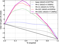
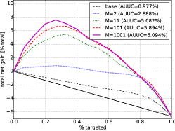
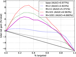
Figure 1: Uplift curves for three uplift boosting algorithms with growing ensemble size for the veteran dataset with E-divergence stump used as base model.

uplift AdaBoost	balanced uplift boosting	balanced forgetting boosting

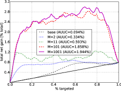
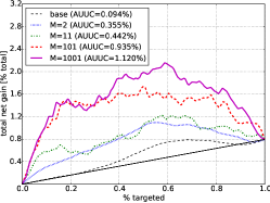
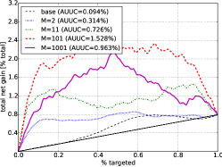
Figure 2: Uplift curves for three uplift boosting algorithms with growing ensemble size for the colon death dataset with three level E-divergence uplift tree used as base model.

Clearly, boosting dramatically improves performance in both cases. For example, for the veteran dataset, the treatment effect is, overall, detrimental with 6% lower survival rate; using just the base model fails to improve the situation. However, if stumps based uplift AdaBoost is used one can select about 35% of the population for whom the treatment is highly beneficial. The overall survival rate can be improved by over 10% (of the total population). One can also see that balanced uplift boosting also resulted in steady increase of performance with the growing ensemble size, but the overall improvement was smaller. For balanced forgetting boosting the performance initially improved, but at some point started to actually decrease. Very similar results can be seen in Figure 2, where boosting also resulted in a dramatic performance increase.

Before discussing those results, we will show Figures 3 and 4 depicting AUUCs for growing ensemble sizes for the three proposed uplift boosting algorithms on all datasets used in our experiments.

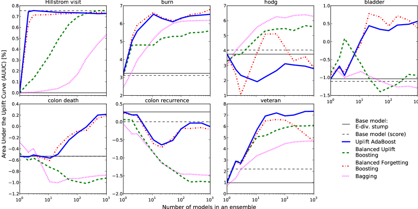
Figure 3: AUUC versus ensemble size for the three proposed uplift boosting algorithms with E-divergence stumps used as base models.

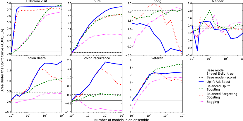
Figure 4: AUUC versus ensemble size for the three proposed uplift boosting algorithms with three level E-divergence trees used as base models.

The figures clearly demonstrate usefulness of boosting which usually outperforms the base models and bagging, often dramatically. Two exceptions are the hodg dataset and the bladder dataset with three level trees used as base learners for which bagging has an advantage over all variants of boosting. On those datasets as well as on Hillstrom visit and colon recurrence with stumps boosting did not improve over the base models. On the Hillstrom visit dataset boosting did dramatically improve on the base models’ 0-1 predictions but not on its scores, which deserves a comment. The mailing campaign was overall effective so the base model’s 0-1 predictions are always 1 giving a diagonal uplift curve and zero AUUC (recall that we subtract the area under the diagonal). There seems to be only one predictive attribute in the data so stumps produced excellent scores which were matched by boosted 0-1 stumps. In this sense boosting probably did find an optimal model in this case.

Interesting cases are the bladder and colon death datasets with uplift stumps used as base models and colon recurrence with three level uplift trees, where uplift AdaBoost and balanced forgetting boosting were able to achieve good performance even though the base model has negative AUUC. This was not the case for bagging and balanced uplift boosting.

Let us now compare the three proposed uplift boosting algorithms. No single algorithm produces the best results in all cases. It can however be seen that typically uplift AdaBoost and balanced forgetting boosting outperform balanced uplift boosting. One can conclude that the property of forgetting the last member added to the ensemble is important, probably because it leads to higher ensemble diversity.

Unfortunately, the balanced forgetting boosting, which performs well for smaller ensembles often begins deteriorating when the ensemble grows too large. We conjecture that the reason is that the bound on the uplift analogue of classification error (Equation 15) is not guaranteed to decrease (see Section 3.3). The performance of the two other uplift boosting algorithms is much more stable in this respect.

Balance seems to be a less important condition. However there is also a possibility that balance is indeed important but uplift AdaBoost does, in practice, maintain approximate balance between treatment and control groups. To investigate this issue we computed the value

$$\max_{m=1,\ldots,101}\max\left\{\frac{p^{T}_{m}}{p^{C}_{m}},\frac{p^{C}_{m}}{p^{T}_{m}}\right\}$$

for uplift AdaBoost for each dataset and base model. The value gives us the largest relative difference between the weight of treatment and control groups over the first 101 iterations. The largest values were obtained for the hodg dataset with stumps ($6.56$) and burn ($24.50$), hodg ($10.93$), veteran ($7.28$) with three level uplift trees; for all other datasets and base models the value was below $2.3$. One can see in Figures 3 and 4 that (except for burn) those are the datasets for which balanced uplift boosting outperformed uplift AdaBoost. Balanced forgetting boosting also performed well on those datasets, at least until its performance started to degrade with larger ensemble sizes.

We thus conclude that balance is in fact important, however in many practical cases the boosting process does not violate it too much and countermeasures are not necessary. There are, however, situations where this is not the case and uplift boosting which explicitly maintains balance is preferred.

5 Conclusions

In this paper we have developed three boosting algorithms for the uplift modeling problem. We began by formulating three properties which uplift boosting algorithms should have. Since all three cannot be simultaneously satisfied, we designed three algorithms, each satisfying two of the properties. The properties of the proposed algorithms are briefly summarized in Table 3.

Table 3: Properties of the proposed uplift boosting algorithms.

	nonincreasing		forgetting
Algorithm	training error bound	balance	the last member
uplift AdaBoost	Yes	No	Yes
balanced uplift boosting	Yes	Yes	No
balanced forgetting boosting	No	Yes	Yes

Experimental evaluation showed that boosting has the potential to dramatically improve the performance of uplift models and typically performs significantly better than bagging. Of the three algorithms uplift AdaBoost usually (but not always) performed best. This is most probably due to the forgetting and training error reduction properties it satisfies. A more thorough analysis revealed that the balance condition, which uplift AdaBoost does not satisfy explicitly, is often satisfied approximately; when this is not the case, other uplift boosting algorithms, especially balanced uplift boosting, are more appropriate. The balanced forgetting boosting which satisfies the balance property and also forgets the last ensemble member does not guarantee the decrease of training error bound. As a result, the algorithm performs well for small ensembles but diverges as more members are added.

Appendix A.

Proof.

(of Theorem 1) Note that the assumption of random group assignment implies $P^{T}(h=1)=P^{C}(h=1)=P(h=1)$ since both groups are scored with the same model and have the same distributions of predictor variables. Using the balance condition, the error $\epsilon$ of $h$, defined in Equation 5, can be expressed as (the second equality follows from $p^{T}=p^{C}=\frac{1}{2}$)

$$2\epsilon =2P^{T}(h=1-y)p^{T}+2P^{C}(h=y)p^{C}=P^{T}(h=1-y)+P^{C}(h=y)$$

$$=P^{T}(h=1,y=0)+P^{T}(h=0,y=1)+P^{C}(h=y=0)+P^{C}(h=y=1)$$

$$=P^{T}(y=0|h=1)P^{T}(h=1)+P^{T}(y=1|h=0)P^{T}(h=0)$$

$$\qquad\qquad+P^{C}(y=1|h=1)P^{C}(h=1)+P^{C}(y=0|h=0)P^{C}(h=0).$$

Using the assumption of random treatment assignment and rearranging:

$$=P(h=1)\left[P^{T}(y=0|h=1)+P^{C}(y=1|h=1)\right]$$

$$\qquad\qquad+P(h=0)\left[P^{T}(y=1|h=0)+P^{C}(y=0|h=0)\right]$$

$$=P(h=1)\left[1-P^{T}(y=1|h=1)+P^{C}(y=1|h=1)\right]$$

$$\qquad\qquad+P(h=0)\left[P^{T}(y=1|h=0)+1-P^{C}(y=1|h=0)\right]$$

$$=1+P(h=1)\left[-(P^{T}(y=1|h=1)-P^{C}(y=1|h=1))\right]$$

$$\qquad\qquad+P(h=0)\left[P^{T}(y=1|h=0)-P^{C}(y=1|h=0)\right].$$

After taking $\epsilon=\frac{1}{2}$ the result follows. ∎

Appendix B.

Here we provide a proof of Theorem 2. First we introduce a lemma establishing relations between $\beta_{m}^{C}$ and $\beta_{m}^{T}$:

Lemma 1.

The following equivalence holds:

$$\beta_{m}^{C}\geq\beta_{m}^{T}\Leftrightarrow\left(\epsilon_{m}^{C}\geq\epsilon_{m}^{T}\land\beta_{m}^{C}\in[1,+\infty)\right)\lor\left(\epsilon_{m}^{C}\leq\epsilon_{m}^{T}\land\beta_{m}^{C}\in(0,1]\right).$$ (24)

Proof.

From Equation 19 we conclude that $\beta_{m}^{C}\geq\beta_{m}^{T}$ is equivalent to $(1-a_{m})\beta_{m}^{C}\geq b_{m}$. Also note that $b_{m}/(1-a_{m})=1$. Clearly

$$\beta_{m}^{C}\geq\beta_{m}^{T}\Leftrightarrow\underbrace{(\beta_{m}^{C}\geq\beta_{m}^{T}\wedge\epsilon_{m}^{C}>\epsilon_{m}^{T})}_{(a)}\vee\underbrace{(\beta_{m}^{C}\geq\beta_{m}^{T}\wedge\epsilon_{m}^{C}<\epsilon_{m}^{T})}_{(b)}\vee\underbrace{(\beta_{m}^{C}\geq\beta_{m}^{T}\wedge\epsilon_{m}^{C}=\epsilon_{m}^{T})}_{(c)}.$$

Condition (a) is equivalent to $(1-a_{m})\beta_{m}^{C}\geq b_{m}\wedge\epsilon_{m}^{C}>\epsilon_{m}^{T}\wedge 1-a_{m}>0$ which in turn is equivalent to $\beta_{m}^{C}\geq 1\wedge\epsilon_{m}^{C}>\epsilon_{m}^{T}$. Similarly (b) is equivalent to $\beta_{m}^{C}\leq 1\wedge\epsilon_{m}^{C}<\epsilon_{m}^{T}$. For (c), notice that $e_{m}^{C}=e_{m}^{T}\Leftrightarrow\beta_{m}^{C}=\beta_{m}^{T}$ (Equation 19) so the right hand side of Equation 24 becomes $\beta_{m}^{C}\in(0,+\infty)\wedge e_{m}^{C}=e_{m}^{T}$, which is trivially true by nonnegativity of $\beta_{m}^{C}$. The result follows after taking the conjunction

$$(\beta_{m}^{C}\geq 1\wedge\epsilon_{m}^{C}>\epsilon_{m}^{T})\vee(\beta_{m}^{C}\leq 1\wedge\epsilon_{m}^{C}<\epsilon_{m}^{T})\vee(\beta_{m}^{C}\in(0,+\infty)\wedge e_{m}^{C}=e_{m}^{T}).$$

∎

It is easy to see that the complementary condition is:

$$\beta_{m}^{C}<\beta_{m}^{T}\Leftrightarrow\left(\epsilon_{m}^{C}<\epsilon_{m}^{T}\land\beta_{m}^{C}\in(1,+\infty)\right)\lor\left(\epsilon_{m}^{C}>\epsilon_{m}^{T}\land\beta_{m}^{C}\in(0,1)\right).$$ (25)

Proof.

(of Theorem 2) Consider two cases: $\beta_{m}^{C}<\beta_{m}^{T}$ and $\beta_{m}^{C}\geq\beta_{m}^{T}$. Assume first, that $\beta_{m}^{C}<\beta_{m}^{T}$. We have

$$f\left(\beta_{m}^{C}\right)=f^{C<T}\left(\beta_{m}^{C}\right)=\frac{1-(1-\epsilon_{m}^{C})(1-\beta_{m}^{C})}{\sqrt{\beta_{m}^{C}}}.$$

Obviously $f^{C<T}\left(1\right)=1$. Now we take the derivative:

$$\frac{df^{C<T}}{d\beta_{m}^{C}}=\frac{(1-\epsilon_{m}^{C})\sqrt{\beta_{m}^{C}}-\frac{1}{2\sqrt{\beta_{m}^{C}}}(\epsilon_{m}^{C}+\beta_{m}^{C}-\epsilon_{m}^{C}\beta_{m}^{C})}{\beta_{m}^{C}},$$

and by equating to zero find a local minimum at

$$\beta_{m}^{C}=\frac{\epsilon_{m}^{C}}{1-\epsilon_{m}^{C}},\qquad\beta_{m}^{T}=\frac{2\epsilon_{m}^{C}-\epsilon_{m}^{T}}{1-\epsilon_{m}^{T}}.$$

Since the numerator of the derivative is a linear function of $\beta_{m}^{C}$, this is also a global minimum of $f^{C<T}$.

Consider now the second case: $\beta_{m}^{C}\geq\beta_{m}^{T}$. Analogously we have

$$f^{C\geq T}\left(\beta_{m}^{C}\right)=\frac{1-(1-\epsilon_{m}^{C})(1-\beta_{m}^{C})}{\sqrt{a_{m}\beta_{m}^{C}+b_{m}}},$$

with $f^{C\geq T}\left(1\right)=1$ and a global minimum at

$$\beta_{m}^{C}=\frac{2\epsilon_{m}^{T}-\epsilon_{m}^{C}}{1-\epsilon_{m}^{C}},\qquad\beta_{m}^{T}=\frac{\epsilon_{m}^{T}}{1-\epsilon_{m}^{T}},$$

provided that $\sqrt{a_{m}\beta_{m}^{C}+b_{m}}>0$. This, however, is always true for the optimal $\beta_{m}^{C}$. Hence, the objective function can be defined as:

$$f(\beta_{m}^{C})=\left\{\begin{array}[]{ll}f^{C\geq T}(\beta_{m}^{C})&if\;\beta_{m}^{C}\geq\beta_{m}^{T},\\ f^{C<T}(\beta_{m}^{C})&if\;\beta_{m}^{C}<\beta_{m}^{T},\\ 1&if\;\beta_{m}^{C}=1.\end{array}\right.$$

We assume strict inequalities between errors and $\frac{1}{2}$, otherwise the optimum is at $\beta_{m}^{C}=\beta_{m}^{T}=1$ with $f(1)=1$. To minimize this function we are going to consider several cases:

1. $\epsilon_{m}^{C}\leq\epsilon_{m}^{T}<\frac{1}{2}$. If $\beta_{m}^{C}\in(0,1]$ we have $\beta_{m}^{C}\geq\beta_{m}^{T}$ (from Lemma 1) so $f(\beta_{m}^{C})=f^{C\geq T}(\beta_{m}^{C})$ and the optimum is at $\beta_{m}^{C*}=\frac{2\epsilon_{m}^{T}-\epsilon_{m}^{C}}{1-\epsilon_{m}^{C}}$. Since $\epsilon_{m}^{C}<2\epsilon_{m}^{T}<1$ we have $0<\beta_{m}^{C*}<1$ and there is a local minimum of $f$ in $\beta_{m}^{C*}$.

   If $\beta_{m}^{C}\in(1,+\infty)$ we have $\beta_{m}^{C}<\beta_{m}^{T}$ (from Lemma 1) so $f(\beta_{m}^{C})=f^{C<T}(\beta_{m}^{C})$. Since the optimum of $f^{C<T}$ is in $\frac{\epsilon_{m}^{C}}{1-\epsilon_{m}^{C}}<1$, $f$ is increasing on $(1,+\infty)$ with minimum at $f(1)=1$.

   Thus we have only one minimum of the objective function $f$ in the whole domain, which is in $\beta_{m}^{C*}$. The corresponding upper bound is $f(\beta_{m}^{C*})=2\sqrt{\epsilon_{m}^{T}(1-\epsilon_{m}^{T})}$.

2. $\frac{1}{2}<\epsilon_{m}^{C}<\epsilon_{m}^{T}$. All derivations are analogous to the previous case, but now the functions: $f^{C\geq T}$, $f^{C<T}$ have their minima taken over $(1,+\infty)$. Hence, only $\beta_{m}^{C*}=\frac{\epsilon_{m}^{C}}{1-\epsilon_{m}^{C}}>1$ is a valid minimum of $f$ on $(0,+\infty)$. The upper bound is now: $f(\beta_{m}^{C*})=2\sqrt{\epsilon_{m}^{C}(1-\epsilon_{m}^{C})}$.

3. $\epsilon_{m}^{T}<\epsilon_{m}^{C}<\frac{1}{2}$. The proof is similar to cases 1 and 2, minimum equal to $2\sqrt{\epsilon_{m}^{C}(1-\epsilon_{m}^{C})}$.

4. $\frac{1}{2}<\epsilon_{m}^{T}<\epsilon_{m}^{C}$. The proof is similar to cases 1 and 2, minimum equal to $2\sqrt{\epsilon_{m}^{T}(1-\epsilon_{m}^{T})}$.

5. $\epsilon_{m}^{C}<\frac{1}{2}<\epsilon_{m}^{T}$. Now $f(\beta_{m}^{C})=f^{C\geq T}(\beta_{m}^{C})$ for $\beta_{m}^{C}\in(0,1]$ and $f(\beta_{m}^{C})=f^{C<T}(\beta_{m}^{C})$ for $\beta_{m}^{C}\in(1,+\infty)$. Yet, the optimum for the first case is in $\frac{2\epsilon_{m}^{T}-\epsilon_{m}^{C}}{1-\epsilon_{m}^{C}}>1$ and for the second in $\frac{\epsilon_{m}^{C}}{1-\epsilon_{m}^{C}}<1$. Since both optima are outside the ranges implied by Lemma 1, the minimum is at $f(1)=1$.

6. $\epsilon_{m}^{T}<\frac{1}{2}<\epsilon_{m}^{C}$. Proof analogous to case 5.

∎

References

- [1] I. Csiszar and P. Shields. Information theory and statistics: A tutorial. Foundations and Trends in Communications and Information Theory, 1(4):417––528, 2004.
- [2] Y. Freund and R.E. Schapire. A decision-theoretic generalization of on-line learning and an application to boosting. Journal of Computer and System Sciences, 55(1):119–139, 1997.
- [3] L. Guelman, M. Guillén, and A.M. Pérez-Marín. Random forests for uplift modeling: An insurance customer retention case. In Modeling and Simulation in Engineering, Economics and Management, volume 115 of Lecture Notes in Business Information Processing (LNBIP), pages 123–133. Springer, 2012.
- [4] L. Guelman, M. Guillén, and A.M. Pérez-Marín. A survey of personalized treatment models for pricing strategies in insurance. Insurance: Mathematics and Economics, 58:68–76, 2014.
- [5] B. Hansotia and B. Rukstales. Incremental value modeling. Journal of Interactive Marketing, 16(3):35–46, 2002.
- [6] K. Hillstrom. The MineThatData e-mail analytics and data mining challenge. MineThatData blog, http://blog.minethatdata.com/2008/03/minethatdata-e-mail-analytics-and-data.html, 2008. Retrieved on 06.10.2014.
- [7] P.W. Holland. Statistics and causal inference. Journal of the American Statistical Association, 81(396):945–960, December 1986.
- [8] S. Jaroszewicz and P. Rzepakowski. Uplift modeling with survival data. In ACM SIGKDD Workshop on Health Informatics (HI-KDD’14), New York, August 2014.
- [9] M. Jaśkowski and S. Jaroszewicz. Uplift modeling for clinical trial data. In ICML 2012 Workshop on Machine Learning for Clinical Data Analysis, Edinburgh, Scotland, June 2012.
- [10] V. Lo. The true lift model - a novel data mining approach to response modeling in database marketing. SIGKDD Explorations, 4(2):78–86, 2002.
- [11] D. Pechyony, R. Jones, and X. Li. A joint optimization of incrementality and revenue to satisfy both advertiser and publisher. In WWW 2013 Companion Publication, pages 123–124, 2013.
- [12] N.J. Radcliffe and P.D. Surry. Real-world uplift modelling with significance-based uplift trees. Portrait Technical Report TR-2011-1, Stochastic Solutions, 2011.
- [13] J. Robins and A. Rotnitzky. Estimation of treatment effects in randomised trials with non-compliance and a dichotomous outcome using structural mean models. Biometrika, 91(4):763–783, 2004.
- [14] P. Rzepakowski and S. Jaroszewicz. Decision trees for uplift modeling. In Proc. IEEE International Conference on Data Mining (ICDM), pages 441–450, Sydney, December 2010.
- [15] P. Rzepakowski and S. Jaroszewicz. Decision trees for uplift modeling with single and multiple treatments. Knowledge and Information Systems, 32:303–327, August 2012.
- [16] R. Schapire. The strength of weak learnability. Machine Learning, 5(2):197–227, July 1990.
- [17] R. Schapire and Y. Singer. Improved boosting algorithms using confidence-rated predictions. Machine learning, 37(3):297–336, 1999.
- [18] M. Sołtys, S. Jaroszewicz, and P. Rzepakowski. Ensemble methods for uplift modeling. Data Mining and Knowledge Discovery, 29(6):1531–1559, 2015.
- [19] S. Vansteelandt and E. Goetghebeur. Causal inference with generalized structural mean models. Journal of the Royal Statistical Society B, 65(4):817––835, 2003.
- [20] G. I. Webb. Multiboosting: A technique for combining boosting and wagging. Machine Learning, 40:159–196, 2000.