Neutron lifetime puzzle and neutron – mirror neutron oscillation

Abstract

The discrepancy between the neutron lifetimes measured in the beam and trap experiments can be explained via the neutron $n$ conversion into mirror neutron $n^{\prime}$, its dark partner from parallel mirror sector, provided that $n$ and $n^{\prime}$ have a tiny mass splitting order $10^{-7}$ eV. In large magnetic fields used in beam experiments $n-n^{\prime}$ transition is resonantly enhanced and can transform of about a per cent fraction of neutrons into mirror neutrons which decay in invisible mode. Thus less protons will be produced and the measured value $\tau_{\rm beam}$ appears larger than $\beta$-decay time $\tau_{\beta}=\tau_{\rm trap}$. Some phenomenological and astrophysical consequences of this scenario are also briefly discussed.

1. Exact determination of the neutron lifetime remains a problem. It is measured in two types of experiments. The trap experiments measure the disappearance rate of the ultra-cold neutrons (UCN) counting the survived UCN after storing them for different times in material or magnetic traps, and determine the neutron decay width $\Gamma_{n}=\tau_{n}^{-1}$. The beam experiments are the appearance experiments, measuring the width of $\beta$-decay $n\rightarrow pe\bar{\nu}_{e}$, $\Gamma_{\beta}=\tau_{\beta}^{-1}$, by counting the produced protons in the monitored beam of cold neutrons. As far as in the Standard Model (SM) the neutron decay always produces a proton, both methods should measure the same value, $\Gamma_{n}=\Gamma_{\beta}$. However, as it was pointed out in Refs. Serebrov:2011 , the tension is mounting between the results obtained by two methods. At present, the experimental results using the trap Mampe:1993 ; Serebrov:2005 ; Pichlmaier:2010 ; Steyerl:2012 ; Arzumanov:2015 ; Serebrov:2017 ; Ezhov:2014 ; Pattie:2017 and the beam Byrne:1996 ; Yue:2013 methods separately yield

$$\tau_{\rm trap}=879.4\pm 0.5~{}{\rm s}$$ (1)

$$\tau_{\rm beam}=888.0\pm 2.0~{}{\rm s}$$ (2)

with the discrepancy of about $4\sigma$: $\Delta\tau=\tau_{\rm beam}-\tau_{\rm trap}=(8.6\pm 2.1)$ s. Barring the possibility of uncontrolled systematic errors and considering the problem as real, then a new physics must be invoked which could consistently explain the relations between the decay width $\Gamma_{n}$, $\beta$-decay rate $\Gamma_{\beta}$, and the measured values (1) and (2).

Some time ago I proposed a way out INT assuming that the neutron has a new decay channel $n\rightarrow n^{\prime}X$ into a ‘dark neutron’ $n^{\prime}$ and some light bosons $X$ among which a photon, due to a mass gap $m_{n}-m_{n^{\prime}}\simeq 1$ MeV (see also Fornal ). Then the beam and trap methods would measure correspondingly the neutron $\beta$-decay rate $\Gamma_{\beta}=\tau_{\rm beam}^{-1}$ and the total width $\Gamma_{n}=\Gamma_{\beta}+\Gamma_{\rm new}=\tau_{\rm trap}^{-1}$, so that $\tau_{\rm trap}/\tau_{\rm beam}$ discrepancy between (1) and (2) could be explained by a branching ratio $\Gamma_{\rm new}/\Gamma_{n}\simeq 0.01$.

However, as it was argued recently in Ref. f2 , such a solution is disfavored by recent experiments Mund ; UCNA that measured $\beta$-asymmetry parameter using different techniques (the cold and ultra-cold neutrons respectively). Their results are in perfect agreement and determine the axial current coupling $g_{A}$ with one per mille precision:

$$g_{A}=1.2755\pm 0.0011\,.$$ (3)

In the SM frames $\tau_{\beta}$ and $g_{A}$ are related as

$$\tau_{\beta}(1+3g_{A}^{2})=(5172.0\pm 1.1)~{}{\rm s}$$ (4)

which relation is essentially free from the uncertainties related to radiative corrections f2 . Then, for $g_{A}$ in the range (3), Eq. (4) predicts the neutron $\beta$-decay time

$$\tau_{\beta}^{\rm SM}=879.5\pm 1.3~{}{\rm s}$$ (5)

perfectly agreeing with the value of $\tau_{\rm trap}$ (1) whereas in the dark decay scenario one expects $\tau_{\rm trap}\!<\!\tau_{\beta}\!=\!\tau_{\rm beam}$. Other way around, for $\tau_{\beta}\!=\!\tau_{\rm beam}$ Eq. (4) would imply $g_{A}=1.2681\pm 0.0017$, more than $3.5\sigma$ away from (3). Hence, the dark decay solution in fact replaces $\Delta\tau$ discrepancy by $g_{A}$ inconsistency f2 . The situation does not improve neither by allowing additional non-standard operators involving scalar or tensor currents in $\beta$-decay, and $\tau_{\rm beam}/\tau_{\beta}$ incompatibility remains persistent BBB .

In the present letter I propose a $g_{A}$-consistent solution in which $\tau_{\rm trap}\!=\!\tau_{\beta}\!<\!\tau_{\rm beam}$. I assume that there exists a parallel/mirror hidden sector as a duplicate of our particle sector, so that all known particles: the electron $e$, proton $p$, neutron $n$, etc., have the mass-degenerate dark twins: $e^{\prime}$, $p^{\prime}$, $n^{\prime}$, etc. (for review see Refs. Alice ). No fundamental principle forbids to our neutral particles, elementary as neutrinos or composite as the neutron, to have mixings with their mirror partners. Then $\tau_{\beta}^{\rm SM}/\tau_{\rm beam}$ discrepancy can be explained via neutron–mirror neutron mixing BB-nn' which phenomenon is similar, and perhaps complementary BM , to a baryon number violating ($\Delta{\rm B}\!=\!2$) mixing between the neutron and antineutron Phillips . But, in contrast to the latter, $\Delta{\rm B}\!=\!1$ transition $n\!\rightarrow\!n^{\prime}$ is not severely restricted by existing experimental bounds and can be rather effective.

2. Consider a theory $G_{\rm SM}\times G^{\prime}_{\rm SM}$ with two gauge sectors where $G_{\rm SM}$ stands for the SM of ordinary (O) particles and $G^{\prime}_{\rm SM}$ for its duplicate describing mirror (M) particles. The identical forms of their Lagrangians can be ensured by discrete $Z_{2}$ symmetry ${\rm SM}\leftrightarrow{\rm SM}^{\prime}$ under which all O particles (fermions, Higgs and gauge bosons) exchange places with their M partners (‘primed’ fermions, Higgs and gauge bosons). If $Z_{2}$ is exact, then all M particles should be exactly degenerate in mass with their O twins.

There can exist also some feeble interactions between O and M particles, e.g. in the form of effective ${\rm L}$-violating operators $\frac{1}{M}l\phi l^{\prime}\phi^{\prime}$ which induce “active-sterile” mixing between our neutrinos $\nu_{e,\mu,\tau}$ and mirror neutrinos $\nu^{\prime}_{e,\mu,\tau}$ ABS . As for the mixing between the neutron and “sterile” M neutron, $\varepsilon\,\overline{n}n^{\prime}+$ h.c., it can be induced by TeV scale operators $\frac{1}{{\mathcal{M}}^{5}}(\overline{u}\overline{d}\overline{d})(u^{\prime}d^{\prime}d^{\prime})$ with quarks $u,d$ and mirror quarks $u^{\prime},d^{\prime}$ BB-nn' . It violates ${\rm B}$ and ${\rm B}^{\prime}$ separately but conserves the combination ${\rm B}+{\rm B}^{\prime}$. Then, modulo $O(1)$ coefficients depending on the operator structures, one has

$$\varepsilon\sim\frac{\Lambda_{\rm QCD}^{6}}{{\mathcal{M}}^{5}}\sim\left(\frac{1~{}{\rm TeV}}{{\mathcal{M}}}\right)^{5}\times 10^{-10}~{}{\rm eV}\,.$$ (6)

One can envisage a situation when $Z_{2}$ is spontaneously broken e.g. a scalar field $\eta$ which is odd under $Z_{2}$ symmetry, $\eta\rightarrow-\eta$, and couples to O and M Higgses as $\lambda\eta(\phi^{\dagger}\phi-\phi^{\prime\dagger}\phi^{\prime})$ BDM . Then its non-zero VEV gives different contributions to mass terms of $\phi$ and $\phi^{\prime}$ in the Higgs potential and thus induces the difference between the VEVs of the latter. If the coupling $\lambda$ is small, then $Z_{2}$ breaking can be tiny, say $\langle\phi^{\prime}\rangle/\langle\phi\rangle=1+O(10^{-13})$ or so. As far as the Yukawa couplings in two sectors are equal, then O and M quarks and leptons will get slightly different masses.

So, let us consider that $n$ and $n^{\prime}$ have a tiny mass splitting $\Delta m=m_{n}-m_{n^{\prime}}\sim 10^{-7}$ eV which can be positive or negative (Cf. the neutron mass itself is measured with the precision of few eV.) With mass gap being so small, $n-n^{\prime}$ transition is not effective for destabilizing the nuclei BB-nn' , but it will affect $n-n^{\prime}$ oscillation pattern for free neutrons. In particular, the limits of Refs. Experiments from experimental search of $n-n^{\prime}$ oscillation obtained by assuming $\Delta m=0$ are no more strictly applicable.

3. Evolution of $n-n^{\prime}$ system is described Schrödinger equation $id\Psi/dt=H\Psi$ where $\Psi=(\psi^{+}_{n},\psi^{-}_{n},\psi^{+}_{n^{\prime}},\psi^{-}_{n^{\prime}})$ stands for wavefunctions of $n$ and $n^{\prime}$ components in two ($\pm$) polarization states. In background free vacuum conditions $4\times 4$ Hamiltonian has the form $H=H_{0}+H_{\rm dec}$:

$$H_{0}=\left(\begin{array}[]{cc}{\frac{\Delta m}{2}}&{\varepsilon}\\ {\varepsilon}&{-\frac{\Delta m}{2}}\end{array}\right),\quad H_{\rm dec}=-\frac{i}{2}\left(\begin{array}[]{cc}{\Gamma_{\beta}}&{0}\\ {0}&{\Gamma^{\prime}_{\beta}}\end{array}\right)\,.$$ (7)

The average mass of $n$ and ${n^{\prime}}$ is omitted since for $n-n^{\prime}$ oscillation only the mass difference $\Delta m$ is relevant. One can also set $\Gamma^{\prime}_{\beta}=\Gamma_{\beta}$ neglecting a tiny difference between the decay rates of $n$ and $n^{\prime}$.

As far as we are interested in average oscillation probabilities, it is convenient to consider the evolution in the basis of mass eigenstates where $H_{0}$ becomes diagonal:

$$\psi_{1}^{\pm}=c_{0}\psi_{n}^{\pm}+s_{0}\psi_{n^{\prime}}^{\pm}\,,\quad\psi_{2}^{\pm}=-s_{0}\psi_{n}^{\pm}+c_{0}\psi_{n^{\prime}}^{\pm}\,,$$ (8)

with $c_{0}=\cos\theta_{0}$ and $s_{0}=\sin\theta_{0}$, $\theta_{0}$ being $nn^{\prime}$ mixing angle in vacuum which is the same for both $\pm$ polarization states, $\tan 2\theta_{0}=2\varepsilon/\Delta m$. In this way one takes into account also possible decoherence effects in $n-n^{\prime}$ oscillation since the mass eigenstates do not oscillate but just propagate independently. The physical sense is transparent: producing a neutron $n$ with $\pm$ polarization is equivalent to producing mass eigenstates $\psi^{\pm}_{1}$ and $\psi_{2}^{\pm}$ respectively with probabilities $c_{0}^{2}$ and $s_{0}^{2}$. Since $\psi^{\pm}_{1}$ interact as $n$ or $n^{\prime}$ respectively with probabilities $c_{0}^{2}$ and $s_{0}^{2}$, and $\psi^{\pm}_{2}$ interact as $n$ or $n^{\prime}$ with probabilities $s_{0}^{2}$ and $c_{0}^{2}$, then the average probability of finding $n$ after a time $t$ is $P_{nn}=c_{0}^{4}+s_{0}^{4}=1-\frac{1}{2}\sin^{2}2\theta_{0}$, and that of finding $n^{\prime}$ is

$$P_{nn^{\prime}}=1-P_{nn}=\frac{1}{2}\sin^{2}2\theta_{0}=2\frac{\varepsilon^{2}}{\delta m^{2}}\,.$$ (9)

Here $\delta m=\Delta m\sqrt{1+(2\varepsilon/\Delta m)^{2}}=\Delta m/\cos 2\theta_{0}$ is the mass gap between the eigenstates (8). As far as $\varepsilon\ll\Delta m$, we have $\delta m\approx\Delta m$, $\cos\theta_{0}\approx 1$ and $\sin\theta_{0}\approx\theta_{0}\approx\varepsilon/\Delta m$. In addition, since in real experimental situations the neutron free flight time between interactions is small, $t\ll\tau_{\beta}$, we have neglected the neutron decay and corresponding overall factor $\exp(-\Gamma_{\beta}t)$ in these probabilities.

The presence of matter background and magnetic fields introduces an additional term in the Hamiltonian:

$$H_{I}=\left(\begin{array}[]{cc}{V_{n}+\mu_{n}\mbox{\boldmath$B$}\mbox{\boldmath$\sigma$}}&{0}\\ {0}&{V^{\prime}_{n}+\mu^{\prime}_{n}\mbox{\boldmath$B$}^{\prime}\mbox{\boldmath$\sigma$}}\end{array}\right)$$ (10)

which includes the optical potentials $V_{n},V^{\prime}_{n}$ induced by O and M matter, and interactions with respective magnetic fields $B$ and $\mbox{\boldmath$B$}^{\prime}$ BB-nn' . Here $\bm{\sigma}=(\sigma_{x},\sigma_{y},\sigma_{z})$ are the Pauli matrices, $\mu_{n}=-1.913\mu_{N}=6.031\times 10^{-8}$ eV/T is the neutron magnetic moment, and $\mu_{n^{\prime}}\approx\mu_{n}$ is that of mirror neutron. In the following we neglect the presence, if any, of M matter and M magnetic field at the Earth. In addition, since the neutron experiments are performed in perfect vacuum conditions, we neglect also $V_{n}$.

In uniform magnetic field $B$ the spin quantization axis can be taken as the direction of $B$, and the Hamiltonian $H=H_{0}+H_{I}$ acquires a simple form

$$H=\begin{pmatrix}\frac{\Delta m}{2}-\Omega_{B}&0&\varepsilon&0\\ 0&\frac{\Delta m}{2}+\Omega_{B}&~{}0~{}&~{}\varepsilon~{}\\ \varepsilon&0&~{}-\frac{\Delta m}{2}~{}&~{}0~{}\\ 0&\varepsilon&~{}0~{}&~{}-\frac{\Delta m}{2}~{}\end{pmatrix}$$ (11)

where $\Omega_{B}=|\mu_{n}B|=(B/1\,{\rm T})\times 60.31$ neV. In this case the Hamiltonian eigenstates are:

$$\psi_{1B}^{\pm}=c_{B}^{\pm}\psi_{n}^{\pm}+s_{B}^{\pm}\psi_{n^{\prime}}^{\pm}\,,\quad\psi_{2B}^{\pm}=-s_{B}^{\pm}\psi_{n}^{\pm}+c_{B}^{\pm}\psi_{n^{\prime}}^{\pm}$$ (12)

with $c_{B}^{\pm}=\cos\theta_{B}^{\pm}$ and $s_{B}^{\pm}=\sin\theta_{B}^{\pm}$. But now $nn^{\prime}$ mixing angles $\theta_{B}^{\pm}$ depend on polarization:

$$\tan 2\theta_{B}^{\pm}=\frac{2\varepsilon}{\Delta m\mp\Omega_{B}}\,.$$ (13)

Hence, in large magnetic fields, when $\Omega_{B}$ becomes comparable with $\Delta m$, one of the oscillation probabilities $P_{nn^{\prime}}^{\pm}=\frac{1}{2}\sin^{2}2\theta_{B}^{\pm}$ ($+$ or $-$ depending on the sign of $\Delta m$) will be resonantly amplified, a phenomenon resembling the famous MSW effect in the neutrino oscillations.

4. Trap experiments store an initial number of the UCN, count the amount of neutrons survived for different times $t$ and determine their disappearance rate $\Gamma_{\rm st}$ via exponential fit $N_{\rm surv}(t)/N_{\rm in}=\exp(-\Gamma_{\rm st}t)$. In real experimental conditions there are always some additional losses, and one has to accurately estimate and substract their rates for finding the true decay time, $\tau_{n}^{-1}=\Gamma_{\rm st}-\Gamma_{\rm loss}$.

These losses are dominated by the UCN absorption or up-scattering at the wall collisions, with a rate given by a product of the mean loss probability per wall scattering $P$ and the mean frequency of scatterings $f$ averaged over the UCN velocity spectrum in the trap, $\Gamma_{\rm wall}=\langle Pf\rangle$. It is controlled by measuring $\Gamma_{\rm st}$ for different frequencies $f$, using traps of different sizes and varying the UCN velocities. In this way, one can determine $\tau_{n}=\tau_{\rm trap}$ by extrapolating the measured values $\Gamma_{\rm st}$ to zero-scattering limit, also finding the neutron loss factor $P$.

In the experiments with material traps the magnetic field is negligibly small, $\Omega_{B}\ll\Delta m$, and $n-n^{\prime}$ conversion probability is given by Eq. (9). Per each wall collision the neutron would escape the trap with a probability $P_{nn^{\prime}}=\frac{1}{2}\sin^{2}2\theta_{0}\simeq 2\theta_{0}^{2}$ which however should be included in the measured loss factor $P$. In particular, in experiment Serebrov:2005 it was estimated as $P\simeq 2\times 10^{-6}$ (see also Ref. Pokotilovski for more details). This gives a conservative upper limit on $nn^{\prime}$ mixing angle, $\theta_{0}<10^{-3}$ or so.

Let us remark that this limit strictly applies if the mass difference $m_{n^{\prime}}-m_{n}=-\Delta m$ is less than the (positive) potential $V_{n}$ confinining neutrons in the trap. The Latter depends on the wall coating material, and for Fomblin Oil used in experiment Serebrov:2005 it is about $100$ neV. For $m_{n^{\prime}}-m_{n}>100$ neV the trapped UCN can be only in the lighter eigenstates $\psi_{1}^{\pm}$, and so the larger values of $\theta_{0}$ are can also also allowed. This could contribute to anomalous UCN losses in the materials with higher potentials (e.g. $V_{n}=240$ neV for Beryllium) origin of which remains unclear in the context of neutron optics calculations Serebrov:2004 . E.g. taking $\Delta m\simeq-200$ neV and $\theta_{0}\simeq 3\times 10^{-3}$, we get $P_{nn^{\prime}}\simeq 2\times 10^{-5}$, close to the measured loss factor for beryllium traps.

The situation is somewhat different for magnetic traps. E.g. experiment Pattie:2017 uses a trap constructed as a Halbach array of permanent magnets with a surface field of about 1 T and additional externally applied holding field $B_{\perp}\sim 10^{-2}$ T, confining only $-$ polarized neutrons. The true lifetime $\tau_{n}$ is assumed to be in practice equal to the measured $\Gamma_{\rm st}^{-1}$, corrected by small $\Gamma_{\rm loss}$ dominated by microphonic heating (0.23 s). The UCN losses on walls is inferred to occur via the neutron depolarization which is effectively controlled by varying the holding field $B_{\perp}$ and gives less than 0.01 s correction. However, the possibility of the losses due to $n-n^{\prime}$ conversion is not taken into account, due to which per each wall scattering the UCN could escape with a probability $P_{nn^{\prime}}^{-}=\frac{1}{2}\sin^{2}2\theta_{B}^{-}$. For $\Delta m>0$ the non-zero magnetic field can only suppress this probability, $P_{nn^{\prime}}^{-}\simeq 2\theta_{0}^{2}/(1+\Omega_{B}/\Delta m)^{2}<2\theta_{0}^{2}$. For negative $\Delta m$ above $-60$ neV or so, this probability can be resonantly enhanced in the vicinity of walls causing too big losses, but e.g. for $\Delta m\simeq-200$ neV this effect will be negligible. The role of $n-n^{\prime}$ conversion in magnetic traps deserves a careful analysis, but generically one can expect the measured value $\tau_{\rm st}$ to be less than true $\tau_{n}$.

Interestingly, experiments with the material Mampe:1993 ; Serebrov:2005 ; Pichlmaier:2010 ; Steyerl:2012 ; Arzumanov:2015 ; Serebrov:2017 and magnetic Ezhov:2014 ; Pattie:2017 traps yield somewhat different results, $\tau_{\rm mat}=880.2\pm 0.5$ s and $\tau_{\rm magn}=877.8\pm 0.7$ s. It is perhaps premature to consider this discrepancy of about $2.7\sigma$, $\tau_{\rm mat}-\tau_{\rm magn}=2.4\pm 0.9$ s, as real but in principle it can naturally occur in our scenario if $\theta_{0}\simeq 10^{-3}$ or so.

5. As discussed in the introduction, the neutron ‘total’ lifetime $\tau_{n}$ measured in the trap experiments (1) perfectly agrees the Standard Model prediction for $\beta$-decay (5), $\tau_{\rm trap}=\tau_{\beta}^{\rm SM}$. This in fact gives an upper limit on the rate of neutron dark decay INT ; Fornal , and in any case disfavors it as explanation of the neutron lifetime puzzle. Hence, the question remains: once $\tau_{n}$ is indeed the same as $\tau_{\beta}$, why then the measurements of the latter in beam experiments Byrne:1996 ; Yue:2013 gives contradictory result with $\tau_{\rm beam}$ (2) of about one percent larger than $\tau_{\beta}$? There are two possibilities: either some fraction of protons produced in the trap is lost by yet unknown reasons, or in large magnetic fields ($B=5$ T and 4.6 T respectively in beam experiments Byrne:1996 ; Yue:2013 ) some fraction of neutrons transforms into M neutrons then decaying via dark channel as $n^{\prime}\rightarrow p^{\prime}e^{\prime}\bar{\nu}_{e}^{\prime}$, and exactly this is the fraction missing the detection.

Let us discuss the beam experiments (described in details in Refs. Yue:2013 ) also taking into account the effect of $n-n^{\prime}$ oscillation. Their principal scheme is shown in Fig. 1. The narrow beam of cold neutrons passes through the proton trap. At any moment the number of neutrons in the trap is $N_{n}=P^{\rm tr}_{nn}L\int_{A}da\int dvI(v)/v$ and the number of M neutrons is $N_{n^{\prime}}=P^{\rm tr}_{nn^{\prime}}L\int_{A}da\int dvI(v)/v$, where $A$ is the beam cross-sectional area, $L$ is the effective length of the trap, $I(v)$ is the velocity dependent fluence rate and $P^{\rm tr}_{nn}=1-P^{\rm tr}_{nn^{\prime}}$ is the average survival probability of the neutron in the trap. Then the count rate of protons produced by $\beta$-decay $n\rightarrow pe\bar{\nu}_{e}$ inside the trap is

$$\dot{N}_{p}=e_{p}\Gamma_{\beta}P^{\rm tr}_{nn}L\int_{A}da\int dv\frac{I(v)}{v}\,,$$ (14)

$e_{p}$ being the counting efficiency. After passing the proton trap, beam hits the neutron counter, which is ⁶LiF foil, and the reaction products of neutron absorption by ⁶Li, alphas and tritons, are detected with a net count rate

$$\dot{N}_{\alpha}=e_{\alpha}\bar{v}P^{\rm det}_{nn}\int_{A}da\int dv\frac{I(v)}{v}\,,$$ (15)

where $e_{\alpha}$ is the counting efficiency normalized to the neutrons with a velocity $\bar{v}=2200$ m/s, and $P^{\rm det}_{nn}=1-P^{\rm det}_{nn^{\prime}}$ is the neutron survival probability at the position of the neutron detector. Hence, by taking the ratio of (14) and (15), in reality one measures not $\tau_{\beta}$ but the value

$$\tau_{\rm beam}=\left(\frac{e_{p}L}{e_{\alpha}\bar{v}}\right)\left(\frac{\dot{N}_{\alpha}}{\dot{N}_{p}}\right)=\frac{P_{nn}^{\rm det}}{P_{nn}^{\rm tr}}\,\tau_{\beta}\,.$$ (16)

Thus, a per cent discrepancy between the measured value $\tau_{\rm beam}$ (2) and the SM predicted $\tau_{\beta}$ (5) can be understood provided that $P_{nn}^{\rm tr}/P_{nn}^{\rm det}\simeq 0.99$, or $P_{nn^{\prime}}^{\rm tr}-P_{nn^{\prime}}^{\rm det}\simeq 10^{-2}$.

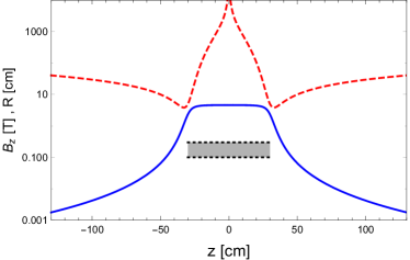
Figure 1: Upper panel: The cold neutron beam passes through the proton trap located inside a solenoid (grey box) inducing magnetic field with the central value $B_{\rm tr}=4.6$ T, and then hits the neutron detector. The red dotted, blue dashed and black solid curves respectively show the evolution of $P_{nn^{\prime}}^{\pm}(z)$ and their average $P_{nn^{\prime}}(z)$ for the parameters chosen as $\theta_{0}=10^{-3}$ and $\Delta m=280$ neV. Lower panel: Profile of the axial magnetic field $B(z)$ induced by continuous solenoid (with length 60 cm and diameter 10 cm) at the position $z$ from its centre. The dashed red curve shows the resonance length scale $R=B\big{(}dB(z)/dz\big{)}^{-1}$ as a function of $z$.

For determining the conversion probabilities $P_{nn^{\prime}}^{\rm tr}$ and $P_{nn^{\prime}}^{\rm det}$, one has to consider the propagation in a variable magnetic field. The field profile induced by a prototype continuous solenoid is shown in Fig. 1. Inside the trap it is $B_{\rm tr}=4.6$ T, quickly falling outside the solenoid. Neutrons are born in small magnetic field and oscillate initially with $P_{nn^{\prime}}^{\rm in}\simeq 2\theta_{0}^{2}$. Then they enter the trap where the field is large and $nn^{\prime}$ mixing angles for $\pm$ polarizations become (13). If evolution of the wavefunction is adiabatic, the mass eigenstates $\psi^{\pm}_{1}$ and $\psi^{\pm}_{2}$ (8) would evolve correspondingly into the “magnetic” eigenstates $\psi^{\pm}_{1B}$ and $\psi^{\pm}_{2B}$ (12) which are detectable as $n$ respectively with the probabilities $c_{B_{\pm}}^{2}$ and $s_{B_{\pm}}^{2}$. Thus, the respective survival probabilities at the coordinate $z$ are fixed by the magnetic field value $B(z)$, $P_{nn}^{\pm}(z)=c_{0}^{2}(c_{B}^{\pm})^{2}+s_{0}^{2}(s_{B}^{\pm})^{2}$. Correspondingly, $n-n^{\prime}$ conversion probabilities are

$$P_{nn^{\prime}}^{\pm}(z)=1-P_{nn}^{\pm}(z)=\frac{1}{2}-\frac{1}{2}\cos 2\theta_{0}\cos 2\theta_{B}^{\pm}(z)$$ (17)

where

$$\cos 2\theta_{B}^{\pm}=\frac{\cos 2\theta_{0}(1\mp\frac{\Omega_{B}}{\Delta m}\big{)}}{\sqrt{\cos^{2}2\theta_{0}(1\mp\frac{\Omega_{B}}{\Delta m}\big{)}^{2}+\sin^{2}2\theta_{0}}}\,.$$ (18)

The evolution of $P_{nn^{\prime}}^{\pm}(z)$ is shown in Fig. 1 for $\theta_{0}=10^{-3}$ and $\Delta m=280$ neV. In this case the evolution is indeed adiabatic, as it can be directly checked by numerically solution of the evolution equation which gives exactly the same result as Eq. (17). The resonance is not crossed, but in the trap the value $\Omega_{B}=|\mu_{n}B|$ approaches $\Delta m$ with about a per cent precision, and $n-n^{\prime}$ conversion probability is strongly amplified for $+$ polarization state, $P_{nn^{\prime}}^{+}(z=0)\approx\frac{1}{2}(1-\cos 2\theta_{B}^{+})\approx 0.02$. Since the neutrons are unpolarized, one should average between two polarizations, $P_{nn^{\prime}}=\frac{1}{2}(P_{nn^{\prime}}^{+}+P_{nn^{\prime}}^{-})$, getting $P_{nn^{\prime}}^{\rm tr}\approx 0.01$. At the neutron detector magnetic field is again small and so $P_{nn^{\prime}}^{\rm det}\approx P_{nn^{\prime}}^{\rm in}\approx 2\theta_{0}^{2}\approx 2\times 10^{-6}$. Then Eq. (16) gives $\tau_{\rm beam}/\tau_{\beta}\approx 1+P_{nn^{\prime}}^{\rm tr}\approx 1.01$. Needless to say, for $\Delta m<0$ the resonant amplification would occur instead for $-$ polarized neutrons but the average probability would remain the same. Thus the sign of $\Delta m$ is irrelevant.

The situation is even more interesting when $\Delta m<260$ neV and the neutron crosses the resonance before entering the proton trap, at some position $z_{\rm res}$ at which $B_{\rm res}=B(z_{\rm res})=|\Delta m/\mu_{n}|=(\Delta m/100~{}{\rm nev})\times 1.66$ T. Eq. (18) tells that $\cos 2\theta^{+}_{B}$ vanishes when $B=B_{\rm res}$ and it becomes negative at $B>B_{\rm res}$. The $-$ polarization states $\psi_{1}^{-}$ and $\psi_{2}^{-}$ still evolve adiabatically respectively into $\psi_{1B}^{-}$ and $\psi_{2B}^{-}$, with $\cos 2\theta^{+}_{B}\approx 1$ and thus $P^{-}_{nn^{\prime}}(z)\leq 2\theta_{0}^{2}$ at any position. But the evolution of $\psi_{1}^{+}$ and $\psi_{2}^{+}$ is no more adiabatic and one has to take into account the Landau-Zener probability that at the resonance crossing the state $\psi_{1}^{+}$ can jump into $\psi_{2B}^{+}$. The goodness of adiabaticity depends on parameter $\xi=\Delta m\sin^{2}2\theta_{0}v^{-1}R(z_{\rm res})$, where $v$ is the neutron velocity. The function $R(z)=\big{(}d\ln B/dz)^{-1}$ (shown in lower panel of Fig. 1) describes the resonance length scale, and it is typically $\sim 10$ cm for $B_{\rm res}\sim 1$ T. Then at coordinates $z$ inside the trap we have

$$P^{+}_{nn^{\prime}}(z)=\frac{1}{2}-\left(\frac{1}{2}-e^{-\pi\xi/2}\right)\cos 2\theta_{0}\cos 2\theta_{B}^{+}(z)$$ (19)

The adiabatic limit (17) corresponds to $\xi\gg 1$. However, in our case $\xi\ll 1$, so that $\exp(-\pi\xi/2)\approx 1-\frac{1}{2}\pi\xi$. In addition, Eq. (18) tells that for $B_{\rm tr}-B_{\rm res}>10^{-2}$ T or so one can take $\cos 2\theta^{+}_{B}\approx-1$. Thus, the conversion probability averaged between $\pm$ polarizations becomes

$$P^{\rm tr}_{nn^{\prime}}\approx\frac{1}{2}P_{nn^{\prime}}^{+}(z=0)\approx\frac{\pi}{4}\xi$$

$$\simeq 10^{-2}\left(\frac{2~{}{\rm km/s}}{v}\right)\left(\frac{\theta_{0}}{10^{-3}}\right)^{2}\left(\frac{B_{\rm res}}{1~{}{\rm T}}\right)\left(\frac{R_{\rm res}}{10~{}{\rm cm}}\right)$$ (20)

just in the range needed for explaining a one per cent difference between $\tau_{\rm beam}$ and $\tau_{\beta}$. Let us recall also that e.g. for $B_{\rm res}=1\div 4$ T, corresponding to $\Delta m=60\div 240$ neV, the resonance length scale $R_{\rm res}=R(z_{\rm res})$ falls in the range of few cm almost independently of the inferred solenoid sizes. (Unfortunately, the detailed descriptions of the magnetic fields used in beam experiments Byrne:1996 ; Yue:2013 are not available, but the profile shown in Fig. 1 is rather similar to that of Fig. 13 in Ref. Yue:2013 .)

In future experiments $n-n^{\prime}$ conversion can be rendered more adiabatic. One can increase the resonance length scale $R_{\rm res}$ by 1-2 orders of magnitude by constructing magnetic fields with smooth enough profile. Then spectacular effect can be expected: in the proton trap almost all neutrons of one polarization will be lost and almost all neutrons of other polarization will survive. So only a half of the initial neutrons will produce protons and the measured $\tau_{\rm beam}$ can appear twice as big as $\tau_{\beta}$.

6. Our scenario suggests interesting connection between the neutron lifetime and dark matter puzzles. Mirror atoms, invisible in terms of ordinary photons but gravitationally coupled to our matter, can constitute a reasonable fraction of cosmological dark matter or even its entire amount. M baryons represent a sort of asymmetric dark matter, and its dissipative character can have specific implications for the cosmological evolution, formation and structure of galaxies and stars, etc. BCV and for dark matter direct detection Cerulli . Interestingly, the same ${\rm B}\!-\!{\rm L}$ (and CP) violating interactions between O and M particles that that induce $\nu-\nu^{\prime}$ or $n-n^{\prime}$ mixings, can induce baryon asymmetries in both O and M worlds in the early universe and naturally explain the dark and visible matter fractions, $\Omega_{{\rm B}^{\prime}}/\Omega_{{\rm B}}\simeq 5$ BB-PRL . There can be some common interactions between two sectors, e.g. with the gauge bosons of the flavor symmetry which can induce oscillation effects between O and M neutral Kaons, etc. which picture also suggests interesting realizations of minimal flavor violation MFV . As for $n-n^{\prime}$ mixing itself, it can have intriguing effects on ultra-high energy cosmic rays propagating at cosmological distances nn'-cosm . Its implications for the neutron stars which can be slowly transformed in mixed O-M neutron stars, with a maximal mass and radii by a factor of $\sqrt{2}$ lower than that of ordinary ones, were briefly discussed in INT and will be analysed in details elsewhere Massimo . It also is tempting to consider the possibility that $n-n^{\prime}$ conversion has some effect in neutron rich heavy unstable nuclides and can be somehow related to the reactor neutrino anomaly Serebrov:2018 .

Some additional remarks are in order. We assumed that mass splitting between ordinary and mirror neutrons, $\Delta m=m_{n^{\prime}}-m_{n}\sim 10^{-7}$ eV, is induced by a tiny breaking of mirror $Z_{2}$ symmetry. Then the same order mass differences can be expected also between O and M protons and electrons, etc. but microphysics of two sectors should be essentially the same. There is nothing wrong in this possibility, and it might be also related to the necessity of asymmetric post-inflationary reheating between O and M sectors BDM . However, there is also a tempting possibility that $Z_{2}$ is exact and $\Delta m=0$, but instead the order $10^{-7}$ eV difference between potentials $V_{n}$ and $V^{\prime}_{n}$ in (10) effectively emerges due to environmental reasons. One can consider some long range 5th forces, with radii comparable to the Earth radius or solar system size, related to e.g. light baryophoton interactions in each sector ABK , or to the difference of graviton/dilaton coupling between O and M components e.g. in the context of bigravity theories bigravity . In first case the force induced by the Earth is repulsive for the neutron which is equivalent of having $\Delta m>0$, while in the second case it would be attractive and equivalent to $\Delta m<0$. This splitting can be effective at the Earth whereas somewhere in cosmological voids it could be vanishingly small.

We considered the effects of $n-n^{\prime}$ mass mixing $\varepsilon$ given in (6), induced by effective $\Delta{\rm B}=1$ interactions between O and M quarks in the context of some new physics, as e.g. seesaw mechanism in Ref. BB-nn' . Generically this underlying physics should violate also CP-invariance, and in principle it can induce interactions with the electromagnetic field Arkady , $\mu_{nn^{\prime}}F_{\mu\nu}\overline{n}\sigma^{\mu\nu}n^{\prime}$ and $d_{nn^{\prime}}F_{\mu\nu}\overline{n}\sigma^{\mu\nu}\gamma^{5}n^{\prime}$ (and equivalent terms with $F_{\nu\nu}\rightarrow F^{\prime}_{\nu\nu}$), where $\mu_{nn^{\prime}}$ and $d_{nn^{\prime}}$ respectively are the transitional magnetic moment and electric dipole moment between $n$ and $n^{\prime}$. Both of these transitional moments can have interesting effects to be studied in details Variano , especially the CP-violating one $d_{nn^{\prime}}$, also because in beam experiments the large electric fields are also used.

To summarize, we discussed a scenario based on $n-n^{\prime}$ conversion which can be effective in large magnetic fields, and can resolve the neutron lifetime puzzle explaining why the beam and trap experiments get different results. In addition, it suggests that the lifetimes measured in material and magnetic traps can be somewhat different, and it can also shed some more light on the origin of the UCN anomalous losses in material traps. Effects for the neutron propagation in matter depend on the sign of $\Delta m$ and deserve careful study. If our proposal is correct, this would mean that installations used in the beam experiments are in fact effective machines that transform the neutrons in dark matter. This can be easily tested experimentally by varying the magnetic field profiles and rendering $n-n^{\prime}$ conversion more adiabatic. In particular, such tests can be done in planned 30 m baseline experiment searching for $n\rightarrow n^{\prime}$ transition and $n\rightarrow n^{\prime}\rightarrow n$ regeneration nn'-exp which is under construction at the HFIR reactor of the Oak Ridge National Laboratory.

Acknowledgements

I thank R. Biondi, Y. Kamyshkov, Y. Pokotilovsky and A. Serebrov for help and useful information.

References

- (1) A. Serebrov and A. Fomin, Phys. Procedia 17, 19 (2011); G. L. Greene and P. Geltenbort, Sci. Am. 314, 36 (2016).
- (2) W. Mampe et al., JETP Lett. 57, 82 (1993).
- (3) A. P. Serebrov et al., Phys. Lett. B 605, 72 (2005); Phys. Rev. C 78, 035505 (2008).
- (4) A. Pichlmaier et al., Phys. Lett. B 693, 221 (2010).
- (5) A. Steyerl et al., Phys. Rev. C 85, 065503 (2012).
- (6) S. Arzumanov et al., Phys. Lett. B 745, 79 (2015).
- (7) A. P. Serebrov et al., Phys. Rev. C 97, 055503 (2018).
- (8) V. F. Ezhov et al., JETP 107, 11 (2018).
- (9) R. W. Pattie, Jr. et al., Science 360, no. 6389, 627 (2018).
- (10) J. Byrne et al., Europhys. Lett. 33, 187 (1996).
- (11) A. T. Yue et al., Phys. Rev. Lett. 111, 222501 (2013); J. S. Nico et al., Phys. Rev. C 71, 055502 (2005).
-
(12)
Z. Berezhiani, ”Unusual effects in conversion”,
talk at the Workshop INT-17-69W, Seattle, 23-27 Oct. 2017,
http://www.int.washington.edu/talks/WorkShops/int_17_69W/People/Berezhiani_Z/Berezhiani3.pdf - (13) B. Fornal and B. Grinstein, Phys. Rev. Lett. 120, 191801 (2018) [arXiv:1801.01124 [hep-ph]].
- (14) A. Czarnecki, W. J. Marciano and A. Sirlin, Phys. Rev. Lett. 120, 202002 (2018) [arXiv:1802.01804 [hep-ph]].
- (15) D. Mund et al., Phys. Rev. Lett. 110, 172502 (2013).
- (16) M. A.-P. Brown et al., Phys. Rev. C 97, 035505 (2018).
- (17) B. Belfatto, R. Beradze and Z. Berezhiani, in preparation
- (18) Z. Berezhiani, Int. J. Mod. Phys. A 19, 3775 (2004); “Through the looking-glass: Alice’s adventures in mirror world,” In I. Kogan Memorial Volume From Fields to Strings, Circumnavigating Theoretical Physics, World Scientific (2005), Eds. M. Shifman et al., vol. 3, pp. 2147-2195 [hep-ph/0508233]; Eur. Phys. J. ST 163, 271 (2008); R. Foot, Int. J. Mod. Phys. A 29, 1430013 (2014).
- (19) Z. Berezhiani and L. Bento, Phys. Rev. Lett. 96, 081801 (2006); Phys. Lett. B 635, 253 (2006); Z. Berezhiani, Eur. Phys. J. C 64, 421 (2009).
- (20) Z. Berezhiani, Eur. Phys. J. C 76, 705 (2016).
- (21) V. Kuzmin, JETP Lett. 12, 335 (1970); R. N. Mohapatra and R. E. Marshak, Phys. Rev. Lett. 44, 1316 (1980); for reviews see D. G. Phillips et al., Phys. Rept. 612, 1 (2016); K. S. Babu et al., arXiv:1310.8593 [hep-ex].
- (22) E. Akhmedov, Z. Berezhiani and G. Senjanovic, Phys. Rev. Lett. 69, 3013 (1992); R. Foot, H. Lew and R. Volkas, Mod. Phys. Lett. A 7, 2567 (1992); R. Foot and R. Volkas, Phys. Rev. D 52, 6595 (1995); Z. Berezhiani and R. N. Mohapatra, Phys. Rev. D 52, 6607 (1995).
- (23) Z. Berezhiani, A. D. Dolgov and R. N. Mohapatra, Phys. Lett. B 375, 26 (1996); Z. Berezhiani, Acta Phys. Polon. B 27, 1503 (1996); R. N. Mohapatra and S. Nussinov, Phys. Lett. B 776, 22 (2018).
- (24) G. Ban et al., Phys. Rev. Lett. 99, 161603 (2007); A. Serebrov et al., Phys. Lett. B 663, 181 (2008); I. Altarev et al., Phys. Rev. D 80, 032003 (2009); A. Serebrov et al., Nucl. Instrum. Meth. A 611, 137 (2009); Z. Berezhiani and F. Nesti, Eur. Phys. J. C 72, 1974 (2012); Z. Berezhiani et al., arXiv:1712.05761 [hep-ex] (Eur. Phys. J. C – in press).
- (25) Y. Pokotilovski, I. Natkaniec and K. Holderna-Natkaniec, Physica B 403, 1942 (2008).
- (26) A. Serebrov et al., Phys. Lett. A 335, 327 (2005).
- (27) Z. Berezhiani, D. Comelli and F. L. Villante, Phys. Lett. B 503, 362 (2001); A. Y. Ignatiev and R. R. Volkas, Phys. Rev. D 68, 023518 (2003); Z. Berezhiani, P. Ciarcelluti, D. Comelli and F. L. Villante, Int. J. Mod. Phys. D 14, 107 (2005); Z. Berezhiani, S. Cassisi, P. Ciarcelluti and A. Pietrinferni, Astropart. Phys. 24, 495 (2006).
- (28) R. Cerulli et al., Eur. Phys. J. C 77, 83 (2017); A. Addazi et al., Eur. Phys. J. C 75, 400 (2015).
- (29) L. Bento and Z. Berezhiani, Phys. Rev. Lett. 87, 231304 (2001); Fortsch. Phys. 50, 489 (2002) [hep-ph/0111116]; Z. Berezhiani, Nucl. Phys. Proc. Suppl. 237-238, 263 (2013); arXiv:1602.08599 [astro-ph.CO].
- (30) Z. Berezhiani, Phys. Lett. B 417, 287 (1998); Z. Berezhiani and A. Rossi, Nucl. Phys. Proc. Sup. 101, 410 (2001).
- (31) Z. Berezhiani and A. Gazizov, Eur. Phys. J. C 72, 2111 (2012); Z. Berezhiani, R. Biondi and A. Gazizov, in press.
- (32) Z. Berezhiani, R. Biondi, M. Mannarelli and F. Tonelli, in preparation
- (33) A. P. Serebrov et al., arXiv:1802.06277 [nucl-ex].
- (34) K. S. Babu and R. N. Mohapatra, Phys. Rev. D 94, 054034 (2016); A. Addazi, Z. Berezhiani and Y. Kamyshkov, Eur. Phys. J. C 77, 301 (2017).
- (35) Z. Berezhiani, F. Nesti, L. Pilo and N. Rossi, JHEP 0907, 083 (2009); Eur. Phys. J. C 70, 305 (2010); see also Z. Berezhiani, D. Comelli, F. Nesti and L. Pilo, Phys. Rev. Lett. 99, 131101 (2007).
- (36) Z. Berezhiani and A. Vainshtein, arXiv:1506.05096 [hep-ph].
- (37) Z. Berezhiani, R. Biondi, Y. Kamyshkov and L. Varriano, in preparation
- (38) L. J. Broussard et al., arXiv:1710.00767 [hep-ex]; see also Z. Berezhiani et al., Phys. Rev. D 96, 035039 (2017).